




1. Introduction
Low back disorders, frequently triggered by repetitive lifting tasks and elevated mechanical loading of the lumbar spine, remain among the most prevalent work-related musculoskeletal injuries (Coenen et al., Reference Coenen, Gouttebarge, Van Der Burght, Van Dieën, Frings-Dresen, Van Der Beek and Burdorf2014; Jahn et al., Reference Jahn, Andersen, Christiansen, Seidler and Dalbøge2023). Excessive flexion-extension angle, moments, and compression forces at the L5-S1 joint are recognized as critical risk factors for the development of chronic low back pain (Murtezani et al., Reference Murtezani, Ibraimi, Sllamniku, Osmani and Sherifi2011; Coenen et al., Reference Coenen, Kingma, Boot, Twisk, Bongers and Van Dieën2013). To better understand these mechanisms, musculoskeletal modeling has become an indispensable tool for estimating internal joint loading and muscle forces, thereby providing a bridge between external motion, force measurements, and spinal kinetics (Abdullah et al., Reference Abdullah, Hulleck, Katmah, Khalaf and El-Rich2024). Such models are central for monitoring biomechanical exposure and informing preventive strategies in occupational ergonomics, rehabilitation, and assistive system design.
A variety of modeling approaches exist. Some rely purely on kinematic and kinetic data obtained from laboratory equipment, while others employ inverse dynamics coupled with static optimization to estimate joint moments and muscle forces (e.g., using the OpenSim framework; Delp et al., Reference Delp, Anderson, Arnold, Loan, Habib, John, Guendelman and Thelen2007). Musculoskeletal modeling, often within multi-body dynamics, is used to represent rigid segments, joint kinematics, and musculotendon actuators for predicting internal loads during complex tasks (such as gait or sit-to-stand maneuvers) (Abdullah et al., Reference Abdullah, Hulleck, Katmah, Khalaf and El-Rich2024). Finite element (FE) musculoskeletal models account for three-dimensional muscle geometry, enabling predictions of muscle contractions and mechanical interactions beyond simple line-segment representations (Li et al., Reference Li, Lu, Miller, Jin and Hua2019; Galbusera et al., Reference Galbusera, Cina, Panico, Albano and Messina2020). Unlike traditional multi-body models, which treat body segments as rigid links connected by idealized joints, FE-based approaches can simulate the deformation of bones, intervertebral discs, and soft tissues under load. This allows for a more detailed assessment of local stress and strain distributions within muscles and spinal structures, providing insights into the mechanical pathways that lead to tissue overload and injury. Such models are particularly useful for studying the internal mechanics of the lumbar spine, as they can account for complex geometries and material heterogeneity of vertebral and disc tissues (Galbusera et al., Reference Galbusera, Cina, Panico, Albano and Messina2020). However, despite their accuracy, FE musculoskeletal models require subject-specific imaging data and high computational resources, limiting their use in dynamic or real-time applications.
Several neuromusculoskeletal modeling approaches integrate EMG-derived muscle activations to estimate muscle forces or joint moments, including the classical EMG-driven models proposed by Buchanan and Lloyd (Lloyd and Besier, Reference Lloyd and Besier2003; Buchanan et al., Reference Buchanan, Lloyd, Manal and Besier2004), hybrid EMG-assisted inverse dynamics frameworks (Shakourisalim et al., Reference Shakourisalim, Martinez, Golabchi, Tavakoli and Rouhani2024). In this context, the calibrated EMG-informed neuromusculoskeletal (CEINMS) framework enables the estimation of joint moments through the integration of kinematic inputs with muscle activation data (Pizzolato et al., Reference Pizzolato, Lloyd, Sartori, Ceseracciu, Besier, Fregly and Reggiani2015). CEINMS has been successfully applied in controlled settings, including lifting tasks, but its implementations have so far remained largely confined to laboratory environments where gold-standard motion capture and force plates are available (Moya-Esteban et al., Reference Moya-Esteban, Van Der Kooij and Sartori2022; Feola et al., Reference Feola, Refai, Costanzi, Sartori and Calanca2023). The same limitation applies to most modeling techniques, whether inverse dynamics or EMG-assisted. This dependence severely limits their applicability in real workplaces, where most hazardous lifting occurs. Occupational risk assessment requires monitoring tools capable of estimating internal spinal loading outside controlled environments.
Recent advances in wearable technologies suggest that the input data required by the CEINMS framework, namely muscle activations and kinematics, can be acquired through wearable sensors, potentially enabling its application outside the lab (Ghamkhar and Kahlaee, Reference Ghamkhar and Kahlaee2015; Papi et al., Reference Papi, Koh and McGregor2017). Surface EMG has long been employed to reveal muscle activation patterns relevant to spinal loading (Geisser et al., Reference Geisser, Ranavaya, Haig, Roth, Zucker, Ambroz and Caruso2005; Lathlean et al., Reference Lathlean, Ramachandran, Sim and Whittle2024), and new approaches, such as inverse synergy methods (Rook et al., Reference Rook, Sartori and Refai2025), highlight the potential to refine EMG-informed models even further.
Static optimization and redundancy-resolution methods used in classical inverse dynamics rely on minimizing a cost function, commonly a function of muscle activation or stress, to predict how muscles share the load around a joint. However, the validity of these assumptions is debated, as the “optimality” criteria may not generalize across different movement types, fatigue states, injury levels, or lifting strategies (Crowninshield and Brand, Reference Crowninshield and Brand1981). EMG-driven models overcome these limitations by using recorded muscle activations, thereby incorporating the subject’s true neuromuscular strategy rather than relying on assumed coordination patterns. This makes EMG-driven modeling particularly important for lifting, where co-contraction, fatigue, and task-specific strategies heavily influence spinal loading.
Wearable inertial motion capture (IMC) systems have emerged as a promising alternative to optoelectronic motion capture (OMC), offering the ability to capture whole-body and trunk kinematics in naturalistic conditions (Palmieri et al., Reference Palmieri, Donno, Cimolin and Galli2023; Motta et al., Reference Motta, Varrecchia, Chini, Ranavolo and Galli2024; Varrecchia et al., Reference Varrecchia, Motta, Chini, Galli and Ranavolo2024; Motta et al., Reference Motta, Chieffo, Monoli, Tuhtan and Galli2025). Several studies have validated IMC against OMC, both for full-body and trunk-level kinematics (Dal Farra et al., Reference Dal Farra, Cerfoglio, Porta, Pau, Galli, Lopomo and Cimolin2025; Villa et al., Reference Villa, Cerfoglio, Bonfiglio, Capodaglio, Galli and Cimolin2025), and more specifically, IMC-based methods have been proposed for estimating L5-S1 joint kinetics (Muller et al., Reference Muller, Mecheri, Corbeil, Plamondon and Robert-Lachaine2022; Nail-Ulloa et al., Reference Nail-Ulloa, Huangfu, Zabala, Bani Hani, Pool, Chen, Schall, Sesek and Gallagher2024).
Hence, although studies have evaluated the use of surface electromyography (sEMG) to measure spine muscle activation and IMC for lifting kinematics, a gap remains in utilizing and validating these two systems against OMC as a source of data for CEINMS to analyze lifting tasks and back load. Bridging this gap could enable the development of a practical tool for assessing workers’ ergonomic risk during lifting tasks through direct measurement and estimation of key biomechanical variables, such as joint angles and moments. Thus, the claim of a “wearable-only model” is novel not in the use of these sensors, but in demonstrating that both the kinematic and the neuromuscular components required by a framework like CEINMS can be derived exclusively from wearable data. This represents a step toward practical on-site risk assessment tools.
This study aims to evaluate if a wearable-only system can be used to estimate L5-S1 flexion moment during a lifting task. The actions carried out for this purpose are: (i) evaluate the estimation of flexion-extension angles at the L5-S1 joint during symmetric lifting tasks using IMC compared to OMC, and (ii) integrate the kinetics from IMC with sEMG data in CEINMS to validate the L5-S1 moment estimates obtained by a wearables-only approach. A systematic comparison will help determine whether CEINMS can be exploited using IMC kinetics and if a wearable-only system can be reliable in joint moment estimation to support ergonomic risk assessment outside laboratory settings.
2. Materials and methods
2.1. Experimental protocol
The study was approved by the Ethical Committee of the University of Twente (ref. 240909). Eight healthy adults (four males, four females; 24 ± 2.5 years; 74.9 ± 11.4 kg; 180 ± 6.4 cm) participated after providing written informed consent. Six bipolar surface EMG electrodes (Cometa, Italy; 2,000 Hz) were placed bilaterally on three back muscles (Longissimus thoracis pars lumborum, Longissimus thoracis pars thoracis, and Iliocostalis), as shown in Figure 1. These muscles were selected because previous literature demonstrated that they are the primary superficial lumbar extensors contributing to L5-S1 flexion-extension moment generation and can be reliably measured using surface EMG (Varrecchia et al., Reference Varrecchia, Conforto, De Nunzio, Draicchio, Falla and Ranavolo2022; Mohamed Refai et al., Reference Mohamed Refai, Moya-Esteban and Sartori2024). Deep muscles such as multifidus were not included due to the limitations of non-invasive EMG acquisition. Maximum voluntary contractions (MVCs) were recorded for normalization. Participants were positioned in a prone position on a treatment table and instructed to perform a maximal isometric trunk extension while an operator applied manual resistance against the upper trunk to oppose the movement. Each MVC lasted approximately 5 s and was repeated three times, with the highest EMG amplitude retained for normalization, following procedures commonly adopted in trunk EMG studies (Vera-Garcia et al., Reference Vera-Garcia, Moreside and McGill2010). Sixty-six retroreflective markers were used, 62 on each participant (modified Cleveland Clinic marker set) (Elliott et al., Reference Elliott, Sawicki, Marecki and Herr2013) and four attached to the corners of the external load (box), acquired at 100 Hz by a 12-camera optical motion capture system (Qualisys, Medical AB, Sweden). In addition, eight inertial measurement units (IMUs; Xsens, Movella, US; 60 Hz) were placed on the upper body according to the manufacturer’s guidelines (Roetenberg et al., Reference Roetenberg, Luinge and Slycke2009). Both markers and IMUs placement are shown in Figure 1.
Markers (pink spheres) and IMUs (orange boxes) placement presented on a scaled model (left), sEMG placement on a participant (center), and schematic representation of the task (right).

Figure 1. Long description
The first panel on the left shows a front and back view of a white human skeleton model. Pink spheres representing Markers are distributed across the joints and limbs, while orange boxes representing I M U s are placed on the sternum, upper arms, forearms, and lower back.
The center panel is a photo of a participant’s back. Eight s E M G sensors are attached to the lower back in two vertical columns of four, positioned on either side of the spine. Each sensor consists of a black circular electrode connected by a white wire to a grey rectangular transmitter.
The right panel is a schematic diagram of a person performing a lifting task. A solid peach-colored figure stands upright holding a blue box labeled LOAD at waist height, marked as START LIFTING. A dashed outline of the figure shows a squatting position reaching for the box on the floor, marked as STOP LIFTING. A green horizontal arrow at the base indicates a distance of 60 cm between the feet and the load.
Ground reaction forces (GRFs) were recorded using a force platform (AMTI, MA; 2,048 Hz). Following IMC calibration, participants performed a static trial and two lifting tasks: stooping (knees extended) and squatting (knees flexed). For each task, four loads (0, 5, 10, and 15 kg) were lifted ten times within 2 min, guided by a metronome. The order of loads and tasks was randomized across participants. Participants lifted the box from the floor to an upright standing posture while holding the load close to the body. The movement ended once the participant reached a fully upright position, resulting in the load being approximately at hip level. The initial box position was standardized on the floor directly in front of the participant’s feet, at a distance of 60 cm, to ensure consistency across trials.
2.2. Data processing
The overall workflow of data processing is summarized in Figure 2. As the first step, marker trajectories were labeled and then processed in OpenSim (OS). For each subject, the Lifting Full Body (LFB) Model was scaled to the static trial. This model was selected because it was specifically developed and validated for the biomechanical analysis of lifting tasks, adding a detailed representation of trunk muscles and lumbar spine mechanics. This makes it particularly suitable for estimating lumbar joint moments during manual material handling (Beaucage-Gauvreau et al., Reference Beaucage-Gauvreau, Robertson, Brandon, Fraser, Freeman, Graham, Thewlis and Jones2019). From the OMC data, the joint angles were estimated using the OS’s inverse kinematics tool.
Data processing workflow. The lines indicate the data processing: in yellow the OMC, in green the IMC, in grey the CEINMS, and in light blue the surface electromyography (sEMG).

Figure 2. Long description
The flowchart is organized into sequential processing blocks connected by color-coded arrows.
1. The process begins on the far left with SCALING MODEL, which receives Static pose markers.
2. This leads to a Scaled Model input for INVERSE KINEMATICS. This block also receives Markers data (yellow) and I M U data (green).
3. The output of INVERSE KINEMATICS is Joint angles, which feed into two parallel blocks: INVERSE DYNAMICS and MUSCLE ANALYSIS.
4. INVERSE DYNAMICS also receives External forces (red) and outputs an L5-S1 Flexion Moment (yellow).
5. MUSCLE ANALYSIS outputs M T U length and Moment arm.
6. These outputs, along with s E M G envelopes normalized (light blue), feed into the C E I N M S CALIBRATION block.
7. The calibration leads to C E I N M S EXECUTION, which produces a second L5-S1 Flexion Moment (black).
8. At the top right, a purple double-headed arrow labeled COMPARISON sits between the yellow O M C-derived L5-S1 Flexion Moment and the black C E I N M S-derived L5-S1 Flexion Moment.
9. A legend in the bottom left identifies the color coding: yellow for O M C, green for I M C, black for C E I N M S, and light blue for s E M G.
For IMC data, IMU locations were determined using the OS IMU Placer tool, which positions virtual sensors on the musculoskeletal model. The tool aligns each sensor with the corresponding body segment by applying a fixed rotation, represented as a direction cosine matrix, that transforms the IMU local reference frame into the segment reference frame. This transformation is defined as

where
$ {R}_{\mathrm{sensor}} $
 is the orientation of the IMU in the global frame, and
$ {R}_{\mathrm{offset}} $
 is the calibration rotation obtained during the static trial, representing the orientation of the sensor with respect to the anatomical segment.
The IMU inverse kinematics tool was then used to compute joint angles by minimizing the difference between measured IMU orientations and the orientations of the corresponding body segments in the musculoskeletal model (Al Borno et al., Reference Al Borno, O’Day, Ibarra, Dunne, Seth, Habib, Ong, Hicks, Uhlrich and Delp2022).
It is important to note that the definition of the L5-S1 joint angle differs between OMC- and IMC-based modeling pipelines. In OMC, the angle is derived from relative marker-based segment orientations within the scaled musculoskeletal model, while in IMC, it is reconstructed from virtual sensor orientations constrained to the corresponding body segments. As a result, the estimated ranges of flexion-extension differ between methods, even for the same movement.
Muscle-tendon lengths and moment arms were obtained via the Muscle Analysis tool, while the flexion moment at the L5-S1 joint was calculated using the Inverse Dynamics tool. Inputs for inverse dynamics included subject kinematics (marker- or IMU-based), box kinematics, and external loads. EMG signals were processed in MATLAB to extract linear envelopes, which were normalized using MVC values.
CEINMS calibration used joint angles (from IMC data), muscle-tendon lengths, moment arms, muscle activations, and IMC-derived joint moments as reference. The musculoskeletal model includes a large set of back muscles modelled by 190 muscle-tendon units (MTUs). EMG signals were recorded only from six muscles, covering 126 MTUs in the model. For the muscles without EMG measurement, only the passive contributions were considered as presented in previous works (Moya-Esteban et al., Reference Moya-Esteban, Van Der Kooij and Sartori2022; Mohamed Refai et al., Reference Mohamed Refai, Moya-Esteban and Sartori2024). To test the ability of the model to generalize across loading conditions, the CEINMS model calibration was performed using only the 0 and 15 kg trials. Once calibrated, CEINMS was executed with the model, muscle-tendon lengths, moment arms, and muscle activations as inputs, yielding L5-S1 joint moments as output.
2.3. Statistical analysis
Each repetition can be divided into five segments based on the lumbo-sacral flexion moment profile. For the analysis, the task was divided into two phases: the first consisting of lowering without weight and lifting with weight, and the second consisting of lowering with weight and lifting without weight (Figure 3). The approach of dividing the analysis between the two phases was chosen based on other literature papers that show differences between lifting the load and lowering it, in terms of biomechanics (Kim, Reference Kim2010), risk to the spine (Larivière et al., Reference Larivière, Gagnon and Loisel2002) and ergonomic reference indices (NIOSH).
Example of one trial of one subject of L5-S1 flexion moment division in the five segments and in the two phases of the task.

Figure 3. Long description
A line graph titled Flexion Moment in the two phases of the task.
Axes and Legend:
The x-axis is Task cycle in percent, ranging from 0 to 100.
The y-axis is L 5 dash S 1 Moment in N m, ranging from 0 to over 200.
The legend identifies a dark blue line as L 5 dash S 1 Moment and five colored background regions: light green for Lowering without weight, blue-grey for Lifting with weight, orange for Standing with weight, purple for Lowering with weight, and light blue for Lifting without weight.
Data Trends:
Phase 1 spans 0 to 45 percent of the cycle. It begins in the light green segment where the moment is near zero until 20 percent, then rises sharply to a peak of approximately 195 N m. It transitions into the blue-grey segment at 35 percent, where an icon shows a person lifting a box with an upward arrow. The moment remains high before dropping sharply toward the end of the phase.
The middle segment from 45 to 55 percent is orange, representing standing with weight, where the moment troughs near zero.
Phase 2 spans 55 to 100 percent of the cycle. It begins in the purple segment where the moment rises sharply again. It transitions into the light blue segment at 70 percent, where an icon shows a person lowering a box with a downward arrow. The moment peaks at approximately 200 N m around 75 percent before declining back to zero by the 95 percent mark.
The comparison of results was conducted from two perspectives: kinematics and dynamics. For the kinematic analysis, the L5-S1 flexion-extension angles derived from OMC and IMC were compared. For the dynamic analysis, a three-way comparison was performed on the L5-S1 flexion moments obtained from three different methods: inverse dynamics (ID) using OMC data (gold standard), ID using IMC data, and CEINMS moments estimated after calibration with IMC data. After verifying the normality of the data, a multi-way ANOVA was conducted to assess the effects of subject, load, and their interaction. Since load was the only factor showing a significant effect, results were averaged across subjects.
3. Results
3.1. Lumbo-sacral flexion angle
Figure 4 depicts the average lumbo-sacral flexion angle over a cycle computed by OMC and IMC systems on all loads and types of lifting. An offset in the starting position is present, with the OMC already flexed at −2°.
Average and standard deviation of L5-S1 flexion angle over a cycle computed by OMC and IMC for each load and type of lifting.

Figure 4. Long description
The multi-panel figure consists of eight line graphs organized into four rows representing loads of 0 K g, 5 K g, 10 K g, and 15 K g. Each row contains two columns: Squat on the left and Stoop on the right.
All graphs share identical axes: the x-axis represents percent Cycle from 0 to 100, and the y-axis represents L 5-S 1 Flexion angle in degrees ranging from -10 to 2. Each plot displays two main lines: a solid line for O M C (Optical Motion Capture) and a dashed line for I M C (Inertial Motion Capture), both accompanied by shaded regions indicating standard deviation.
Data Trends:
- Across all panels, the curves follow a double-peak sinusoidal pattern. The first trough occurs around 25 percent of the cycle, followed by a peak near 50 percent, a second trough near 75 percent, and a final rise toward 100 percent.
- The I M C (dashed line) consistently shows higher flexion angle values (closer to 0 or positive) compared to the O M C (solid line), which remains lower (more negative) throughout the cycles.
- Row 1 (0 K g, Blue): Shows the widest standard deviation bands, particularly for the O M C data during the peaks.
- Row 2 (5 K g, Green): The gap between O M C and I M C remains consistent, with both methods capturing the same rhythmic troughs at approximately -6 degrees.
- Row 3 (10 K g, Orange): The curves are smoother with slightly narrower standard deviation bands compared to the 0 K g load.
- Row 4 (15 K g, Purple): The Stoop condition on the bottom right shows a more pronounced difference in peak height at the 50 percent cycle mark compared to the Squat condition on the left.
In all cases, while the absolute values differ between O M C and I M C, the temporal patterns and inflection points are highly synchronized.
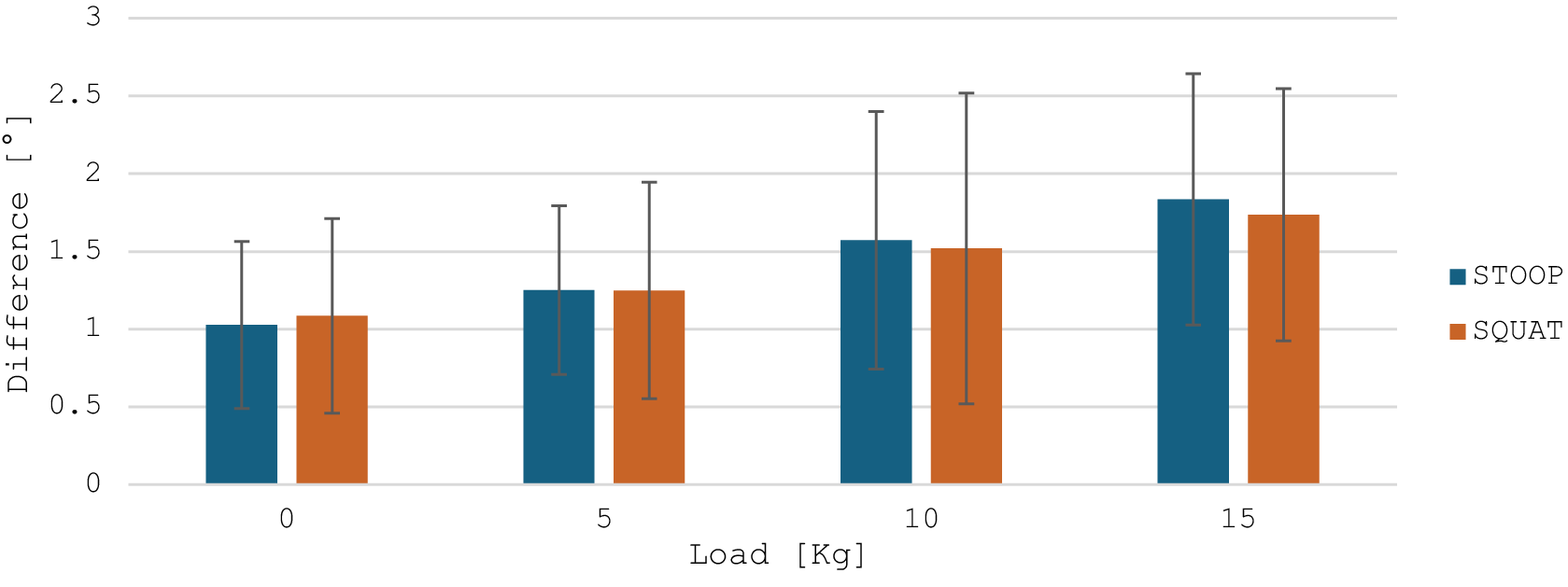
In Figure 5, the average difference and its standard deviation of the maximum L5-S1 flexion angle are reported as a bar plot.
Average and standard deviation of the difference of the maximum L5-S1 flexion angle between OMC and IMC for each load and type of lifting.

Figure 5. Long description
The X-axis is labeled Load in K g with four discrete categories: 0, 5, 10, and 15. The Y-axis is labeled Difference in degrees, ranging from 0 to 3 in increments of 0.5. A legend on the right identifies blue bars as S T O O P and orange bars as S Q U A T.
Data trends show a linear increase in the difference for both lifting types as load increases.
At 0 K g: S T O O P is approximately 1.0 and S Q U A T is approximately 1.1.
At 5 K g: Both S T O O P and S Q U A T are approximately 1.25.
At 10 K g: S T O O P is approximately 1.6 and S Q U A T is approximately 1.5.
At 15 K g: S T O O P is approximately 1.8 and S Q U A T is approximately 1.7.
Each bar includes a vertical error bar representing standard deviation. The error bars are large and overlapping, extending roughly 0.5 to 1.0 units above and below the mean values, with the spread increasing slightly at higher loads.
The mean difference between the two systems is 1.84° ± 0.86°. A one-sample t-test showed that this mean is significantly greater than zero (t = 16.59, p < .001), with a 95% confidence interval ranging from 1.62° to 2.06°. Looking at each load value, the discrepancies range from 1.1° to 2.4°, with slightly larger values observed at higher loads. The difference is always positive, meaning that the IMC underestimates the flexion angle. The variability, represented by the error bars, was limited and consistent across conditions, indicating stable performance of the IMC system in reproducing lumbar flexion angles.
3.2. Lumbo-sacral flexion moment
Table 1 reports the average and standard deviation values of the statistical parameters computed on the entire signals of the L5-S1 moment, comparing the OMC-based ID with IMC-based ID and CEINMS.
Statistical parameters comparing the entire signal of lumbo-sacral flexion moment in the three methods

Table 1. Long description
The table presents five statistical parameters across four load levels: 0 k g, 5 k g, 10 k g, and 15 k g. For each parameter, data is split into STOOP and SQUAT movements, comparing O M C versus I M C and O M C versus CEINMS.
Spearman correlation coefficient (std): For STOOP, O M C versus I M C ranges from 0.90 to 0.94; O M C versus CEINMS ranges from 0.81 to 0.87. For SQUAT, O M C versus I M C ranges from 0.83 to 0.96; O M C versus CEINMS ranges from 0.83 to 0.86.
R M S E (std) in N m: For STOOP, O M C versus I M C stays around 2.62 to 2.89; O M C versus CEINMS increases from 5.52 to 9.75 as load increases. For SQUAT, O M C versus I M C ranges from 2.54 to 3.59; O M C versus CEINMS ranges from 5.61 to 6.75.
Bland-Altman Bias (interval of confidence) in N m: For STOOP, O M C versus I M C bias ranges from 0.06 to 1.70; O M C versus CEINMS ranges from 0.64 to 1.98. For SQUAT, O M C versus I M C bias ranges from 0.02 to 1.96; O M C versus CEINMS ranges from 0.14 to 2.22.
Intraclass correlation (std): Values are high across all categories, generally between 0.87 and 0.98.
Coefficient of multiple correlation (std): Extremely high consistency with values consistently at 0.98 or 0.99 for all loads and methods.
Note: The values are the average and standard deviation of the results for each load value, except for the Bland–Altman Bias and interval of confidence.
The direct comparison between L5-S1 flexion moment estimates obtained through inverse dynamics based on OMC and IMC data revealed a very high level of agreement between the two systems. Spearman correlation coefficients were consistently high across all lifting conditions (0.83–0.96). Reliability indices, including the ICC (ICC > 0.91) and the CMC (CMC ≈ 0.99), further confirmed the robustness of the dynamic reconstruction derived from the inertial sensors. The RMSE, averaging between 2.5 and 3 Nm, indicated good absolute precision with limited variation across loads, while the mean bias remained close to zero, suggesting the absence of systematic over- or underestimation trends. The comparison between OMC-based ID and CEINMS revealed very similar results between the two types of lifting: a strong correlation across all loading conditions, with Spearman coefficients ranging from 0.81 to 0.87. Reliability indices, including ICC (0.87–0.91) and CMC (>0.98), confirmed a high level of consistency and overall profile similarity. Mean bias remained low (0.14–2.22 Nm), suggesting the absence of substantial systematic errors; however, the widening confidence intervals at higher loads indicated increasing variability. Similarly, RMSE values rose from 5.52 to 9.75 Nm, accompanied by larger standard deviations, highlighting a reduction in absolute precision as the applied load increased.
Figure 6 depicts the average lumbo-sacral flexion moment over a cycle computed by ID from OMC and IMC data and computed by CEINMS on all loads and types of lifting. It should be noted that the higher L5-S1 flexion moments observed during squat compared to stoop refer to averaged data. A Mann–Whitney test performed between the max values of the moment between the two lifting techniques resulted in a lack of statistically significant difference. At the individual level, variability was present. The mean standard deviation of the average squat cycle for the OMC data varied from 0.3 Nm/kg at 5 kg of load to 0.7 Nm/kg at 0 kg, and for the stoop from 0.2 Nm/kg at 15 kg to 0.8 Nm/kg at 0 kg. These results highlight the high inter-subject variability and the relative magnitudes of the moments, which depend on each participant’s lifting strategy, particularly the degree of trunk inclination and knee flexion adopted. It shows how there is an offset at the starting position and that the OMC moment is usually higher than the other two.
Average L5-S1 flexion moment over a cycle computed by OMC, IMC, and CEINMS for each load and type of lifting.

Figure 6. Long description
A grid of eight line graphs arranged in four rows and two columns.
Axes and Legend:
The x-axis for all graphs is percent Cycle from 0 to 100.
The y-axis is Normalized L 5-S 1 Flexion Moment in Newton meters per kilogram, ranging from negative 0.5 to 3.
Each graph contains three lines: blue for O M C, orange for I M C, and yellow for CEINMS.
Row 1 (Load: 0 kg):
Left (Squat): All three methods show a bimodal peak between 30 and 80 percent cycle, peaking near 2.0. O M C starts and ends lower (near 0) compared to I M C and CEINMS (near 0.5).
Right (Stoop): Similar bimodal trend, but the peaks are broader and slightly lower, around 1.5.
Row 2 (Load: 5 kg):
Left (Squat): Peaks increase to approximately 2.2 for O M C, while I M C and CEINMS peak lower at 1.8.
Right (Stoop): O M C shows a higher second peak compared to the first, reaching 2.2.
Row 3 (Load: 10 kg):
Left (Squat): O M C peaks reach 2.6, showing a significant vertical divergence from I M C and CEINMS which remain around 2.0.
Right (Stoop): The three methods track more closely than in the squat, with peaks between 2.0 and 2.3.
Row 4 (Load: 15 kg):
Left (Squat): O M C peaks reach their highest point at 2.7. I M C and CEINMS follow a similar shape but peak at 2.3.
Right (Stoop): All three methods show high agreement in the first peak (2.3), with O M C slightly higher in the second peak.
General Trend: As load increases from 0 to 15 kilograms, the magnitude of the flexion moment increases across all methods. O M C consistently records lower baseline values at the start and end of the cycle compared to the other two methods.
Table 2 reports the values of the average difference between the average maximum and mean values of lumbo-sacral moments in a cycle from OMC-based ID with respect to IMC-based ID and CEINMS.
Values of the average (and standard deviation) difference between the maximum and mean values of moment over a cycle by the IMC-based ID and CEINMS compared to OMC-based ID methods during lifting and lowering

Table 2. Long description
A table presenting the average and standard deviation of differences in Newton-meters between O M C based I D and two other methods, I M C and CEINMS, across four load conditions: 0 k g, 5 k g, 10 k g, and 15 k g. The data is divided into four main sections:
1. Difference in max moment during Phase 1: For STOOP lifting, O M C vs. I M C ranges from minus 5.61 to minus 14.78. O M C vs. CEINMS ranges from minus 8.25 to minus 14.44. For SQUAT lifting, O M C vs. I M C ranges from minus 3.28 to minus 12.61, while O M C vs. CEINMS ranges from minus 4.30 to minus 20.79.
2. Difference in max moment during Phase 2: For STOOP, O M C vs. I M C ranges from minus 3.48 to minus 13.76. O M C vs. CEINMS shows an overestimation at 0 k g (2.52) but underestimation at higher loads. For SQUAT, O M C vs. I M C ranges from minus 3.62 to minus 12.36.
3. Difference in mean moment during Phase 1: For STOOP, O M C vs. CEINMS shows overestimation across all loads, peaking at 9.93 for 15 k g. For SQUAT, O M C vs. CEINMS also shows significant overestimation, reaching 17.83 at 15 k g.
4. Difference in mean moment during Phase 2: Values are generally smaller, with STOOP O M C vs. CEINMS showing overestimation at 5, 10, and 15 k g loads. SQUAT O M C vs. CEINMS shows underestimation at most loads, such as minus 3.69 at 5 k g.
Statistically significant differences are marked with an asterisk, and positive values indicate overestimation by the comparison method.
Note: The positive differences, indicating an overestimation, are highlighted in green. The statistically significant differences are reported with an asterisk.
During Phase 1, the maximum moment was almost consistently underestimated by IMC-based ID and CEINMS, as shown by the low number of green cells, with increasing discrepancies at higher loads, especially for CEINMS in squat (from −4.30 Nm at 0 kg to −20.79 Nm at 15 kg). Conversely, during Phase 2, while IMC-based presented a similar trend in Phase 1, differences in maximum moment were smaller for CEINMS in squat (ranging between −0.46 and + 1.88 Nm) and stoop for 0 to 10 kg (−5.57 to 2.52 Nm), with a higher difference only in stoop at 15 kg.
Mean moment analysis revealed heterogeneous outcomes for CEINMS: while differences during Phase 2 remained limited (−3.69 to +5.43 Nm), Phase 1, and especially squat, showed larger discrepancies, particularly at 15 kg (+9.93 Nm in stoop and +17.83 Nm for squat). IMC-based ID instead presents stable, low error across all loads and types of lifting.
Figure 7 shows the average maximum (left) and mean (right) L5-S1 flexion moments normalized over the body weight obtained with the OMC-based ID and CEINMS during the two phases of the stoop and squat task at different loads.
Average maximum (left) and mean (right) values of lumbo-sacral moment for the two types of lifting in the two phases from OMC-based ID and CEINMS for each load.

Figure 7. Long description
A multi-panel figure containing four bar charts arranged in a two-by-two grid. The top row is titled Max and Mean Flexion Moment normalized over body weight - Squat. The bottom row is titled Max and Mean Flexion Moment normalized over body weight - Stoop.
All charts share the same axes: the y-axis is Normalized L 5 - S 1 Flexion Moment in N m forward slash K g, ranging from 0 to 3.5. The x-axis is Load in K g with four categories: 0, 5, 10, and 15. Each load category contains four bars: Phase 1 O M C (solid), Phase 1 C E I N M S (hatched), Phase 2 O M C (solid), and Phase 2 C E I N M S (hatched).
Top-Left (Squat Max): Shows a linear increase in moment as load increases. O M C values for Phase 1 are consistently higher than C E I N M S, reaching nearly 3.0 at 15 K g. Phase 2 values are lower than Phase 1 and show closer agreement between O M C and C E I N M S.
Top-Right (Squat Mean): Shows a similar linear increase but with lower overall magnitudes than the Max chart, peaking around 2.2. There is high agreement between all four bar types across all loads.
Bottom-Left (Stoop Max): Phase 1 O M C (purple) and Phase 2 O M C (yellow) show a steady increase. Phase 1 O M C is consistently higher than its C E I N M S counterpart. At 15 K g, the values plateau around 2.5.
Bottom-Right (Stoop Mean): Displays the lowest overall values, starting around 1.4 at 0 K g and rising to approximately 2.0 at 15 K g. The difference between O M C and C E I N M S is minimal in this panel.
In all cases, flexion moments increased progressively with the external load, as expected. For the maximum values, CEINMS tended to slightly underestimate the moments compared to OMC during lifting, particularly at 10 and 15 kg, whereas differences were smaller and more consistent during lowering. Regarding mean moments, the two systems exhibited closer agreement across all loads, with only minor discrepancies observed at higher loads during lifting. Overall, both systems captured the load-dependent increase in lumbar moments, with the largest deviations occurring for peak values in the lifting phase, while mean values and lowering phases showed higher consistency between methods.
4. Discussion and conclusion
This study shows that the CEINMS framework, combined with IMC and sEMG signals, can provide a robust alternative to gold-standard laboratory approaches for estimating lumbar joint moments. These findings are in line with previous studies reporting root mean square (RMS) errors around 20 Nm and high ICCs in IMU-based estimation of spinal kinetics during trunk bending and manual handling tasks (Faber et al., Reference Faber, Chang, Kingma, Dennerlein and Van Dieën2016; Matijevich et al., Reference Matijevich, Volgyesi and Zelik2021). The present results extend this evidence to symmetric lifting tasks, reinforcing the potential of wearables for ecological assessments outside laboratory environments.
Inverse kinematics and inverse dynamics were performed using OpenSim (Delp et al., Reference Delp, Anderson, Arnold, Loan, Habib, John, Guendelman and Thelen2007; Seth et al., Reference Seth, Hicks, Uchida, Habib, Dembia, Dunne, Ong, DeMers, Rajagopal, Millard, Hamner, Arnold, Yong, Lakshmikanth, Sherman, Ku and Delp2018), a widely adopted and validated framework for musculoskeletal modeling. The use of OpenSim ensured methodological consistency with the musculoskeletal model and facilitated integration with the CEINMS framework (Pizzolato et al., Reference Pizzolato, Lloyd, Sartori, Ceseracciu, Besier, Fregly and Reggiani2015). Importantly, the LFB model employed in this study was specifically developed and validated for lifting tasks within the OpenSim environment (Beaucage-Gauvreau et al., Reference Beaucage-Gauvreau, Robertson, Brandon, Fraser, Freeman, Graham, Thewlis and Jones2019), providing explicit support for the estimation of lumbar spine loads at the L5-S1 joint during symmetric lifting, which directly aligns with the scope of this work. The LFB model includes detailed trunk musculature and lumbar vertebral degrees of freedom, making it particularly suited for the analysis of spinal loading during manual material handling (Beaucage-Gauvreau et al., Reference Beaucage-Gauvreau, Robertson, Brandon, Fraser, Freeman, Graham, Thewlis and Jones2019; Manoharan et al., Reference Manoharan, Pranata, Tse and Chai2023).
Regarding the muscle force estimation framework, it is worth noting that CEINMS is not the sole option for performing EMG-informed neuromusculoskeletal modelling as presented in the introduction chapter. However, CEINMS offers distinct advantages that motivated its adoption in this study: it operates on dynamic skeletal models with any number of degrees of freedom and MTUs, supports multiple neural control solutions (EMG-driven, EMG-assisted, and static optimization) within the same framework, enables subject-specific calibration of neuromuscular parameters, and integrates with OpenSim (Pizzolato et al., Reference Pizzolato, Lloyd, Sartori, Ceseracciu, Besier, Fregly and Reggiani2015). Studies applying a similar pipeline have demonstrated its effectiveness across a range of dynamic tasks, including walking (Bu et al., Reference Bu, MacLean and Ferris2023), cycling (Crossley et al., Reference Crossley, Worsey, Diamond, Saxby, Wackwitz, Bourne, Lloyd and Pizzolato2025), and high-speed locomotion (Akhundov et al., Reference Akhundov, Saxby, Diamond, Edwards, Clausen, Dooley, Blyton and Snodgrass2022), confirming its suitability for tasks involving complex multi-joint coordination. A custom IK/ID pipeline could potentially allow greater control over joint definitions and model assumptions; however, replicating the validated procedures embedded in OpenSim was beyond the scope of this work, and any systematic offset introduced by the standardized pipeline would be consistent across tasks and participants, making it a reproducible and comparable source of variability rather than a task-specific confound.
In addition to the CEINMS validation, the comparison between IMC- and OMC-based ID revealed an excellent level of agreement, as reported in Table 1, confirming the reliability of the IMC system in reproducing lumbar joint kinetics. The strong correlations (ρ = 0.83–0.96) and high reliability indices (ICC > 0.91, CMC ≈ 0.99) indicate that IMC-based estimates can accurately replicate the temporal evolution and magnitude of the L5-S1 flexion moments observed with OMC. The low RMSE (≈2.5–3 Nm) and near-zero bias further suggest that the differences between the two systems are minimal, supporting the feasibility of IMC for standalone use in dynamic lifting analysis. Looking at the moment average graphs (Figure 6), the initial offset in starting values could be due to the offset present at the initial state in the flexion angle, as reported in Figure 4.
A key observation concerns the underestimation of peak flexion moments during the lifting phase, which became more pronounced with heavier loads, as reported in Table 2 and Figure 7 and in accordance with Muller et al. (Reference Muller, Mecheri, Corbeil, Plamondon and Robert-Lachaine2022). This is probably due to the increasing difference in flexion angle as reported in Figure 5 rather than to the recorded muscle activation. In OS, individual intervertebral joint angles are not directly measured. Instead, the model estimates the L5-S1 angle and assumes proportional motion across the other lumbar levels. Therefore, discrepancies between OMC and IMC-based estimates likely arise from differences in segment orientation estimation.
Several factors may contribute to the observed underestimation. First, IMU sensor-fusion and filtering algorithms tend to smooth extreme joint excursions (Morrow et al., Reference Morrow, Lowndes, Fortune, Kaufman and Hallbeck2017; Dal Farra et al., Reference Dal Farra, Cerfoglio, Porta, Pau, Galli, Lopomo and Cimolin2025). Second, small misalignments between sensors and anatomical segments, combined with calibration constraints, can introduce angular biases that propagate non-linearly into joint moment estimation, especially under high external loads (Shakourisalim et al., Reference Shakourisalim, Martinez, Golabchi, Tavakoli and Rouhani2024). Third, soft-tissue artefacts and frame-definition differences can also affect OMC outputs in distinct ways compared with IMC. Increasing sensor density along the lumbar region could enhance the resolution of multi-segmental motion and mitigate some of these error sources (Moon et al., Reference Moon, Gombatto, Phan and Ozturk2022; Beange et al., Reference Beange, Chan and Graham2024).
From an application standpoint, the relatively low bias and high agreement of CEINMS (calibrated from IMC data) across loads highlight the promise of IMUs and sEMG-driven models for ergonomic risk assessment and workplace monitoring. Even if peak loads are slightly underestimated, the wearable approach successfully captured the expected load-dependent increase in lumbar moments, which is the key feature for evaluating relative changes in mechanical exposure across tasks or conditions. This suggests that wearable-driven estimates may be sufficient to identify hazardous lifting scenarios and support preventive interventions in occupational settings.
Interestingly, group-averaged results (Figure 6) showed slightly higher L5-S1 flexion moments during squat compared to stoop, even for the gold-standard OMC. Meaning that these results are not related to CEINMS or even IMC but are a direct cause of the kinematics strategies of the subjects, as reported also in the literature (Van Dieën et al., Reference Van Dieën, Hoozemans and Toussaint1999; Bazrgari et al., Reference Bazrgari, Shirazi-Adl and Arjmand2007; Van Der Have et al., Reference Van Der Have, Van Rossom and Jonkers2019). This may appear counterintuitive, as stoop lifting is often associated with a larger trunk moment arm relative to L5-S1, the effective joint moment depends not only on trunk inclination but also on the overall lifting strategy, including knee flexion, hip contribution, and vertical displacement of the load. Inter-subject variability was observed, and the relative magnitude of squat versus stoop moments was influenced by the actual trunk and knee kinematics adopted. Starting from the L5-S1 flexion angle, which, as reported in Figure 4, showed slightly larger values in squat rather than stoop. This is a direct cause of the increasing moment values. Therefore, these findings should not be interpreted as a general biomechanical rule but rather as task- and strategy-dependent outcomes.
Some limitations should be acknowledged. First, the sample size was small and limited to young, healthy adults, which restricts generalizability to workers of different ages, body compositions, or individuals with musculoskeletal conditions. Second, calibration was performed only at 0 and 15 kg to evaluate the ability of the model to generalize across intermediate loads. An alternative approach would have been to calibrate across all loading conditions to maximize accuracy. However, this would have reduced the possibility of testing its generalization performance. Future studies could compare these calibration strategies to evaluate the trade-off between accuracy and generalizability. Lastly, from an application standpoint, it is important to note that sensor placement accuracy remains a crucial aspect. However, the procedure is straightforward and can be easily learned after minimal training, making it feasible for use in workplace settings. Standardized positioning protocols and quick calibration routines could further enhance repeatability and reduce operator dependency, supporting consistent measurements across different users and environments.
Since the difference in terms of L5-S1 flexion angle ROM is not negligible, future research should focus on improving the accuracy of the IK computed from IMU for such small joints. Moreover, a larger and more diverse population should be explored, including real-world lifting scenarios with variable asymmetry and dynamics, and investigating the integration of multi-sensor lumbar configurations. Moreover, coupling wearable-based kinetic estimates with fatigue or discomfort measures could broaden the applicability of such systems in occupational health.
In conclusion, this study provides strong validation evidence for a wearable-only approach to estimating L5-S1 flexion-extension moments. While peak values during lifting under heavy loads are underestimated, the overall accuracy and reliability are high, supporting the feasibility of using IMUs and sEMG-based neuromusculoskeletal models for field applications in ergonomics and occupational biomechanics.
Abbreviations
- CEINMS
-
calibrated EMG-informed neuromusculoskeletal
- FE
-
finite element
- IMC
-
inertial motion capture
- OMC
-
optoelectronic motion capture system
- OS
-
OpenSim
Data availability statement
Data can be made available to interested researchers upon request by email to the corresponding author.
Authorship contribution
M.S., M.I.R., and F.M. designed the study; F.M. conducted data acquisition and formal analysis; M.S. and M.I.R. supervised data collection and processing; M.S., M.I.R., and F.M. wrote the article; and T.V., M.G., and A.R. revised the manuscript. M.S. and M.G. equally supervised the work.
Funding statement
This work was partly funded by the ERC Consolidator Grant ROBOREACTOR (Grant No. 101123866), the Netherlands Sectorplan Techniek II, and the EU RIA project SWAG (Grant No. 101120408). Open access funding provided by University of Twente.
Competing interests
The authors declare no competing interests exist.
Ethical standards
The authors assert that all procedures contributing to this work comply with the ethical standards of the relevant national and institutional committees on human experimentation and with the Helsinki Declaration of 1975, as revised in 2008.
AI tools use
The authors declare that AI tool (ChatGPT5a) was used on November 10, 2025, only for grammar checks and rephrasing of some sentences, but not for producing completely new text.




 Open access

