

Bipolar disorder (BD), which is characterized by alternating periods of mania and depression, is a severe familial disorder. Five to 10 percent of first-degree relatives of probands with BD will develop BD (reviewed by Craddock & Jones, Reference Craddock and Jones2001), and some estimates suggest the rate of BD in offspring of parents with BD (O-BD) is slightly higher (e.g., Meyer et al., Reference Meyer, Carlson, Wiggs, Martinez, Ronsaville and Klimes-Dougan2004). Previous research has largely focused on identifying precursors of BD. Although the search for risk factors for BD is critically important, studies of associated risks should include a wider spectrum of problems such as the full range of more commonly experienced incapacitating emotional and behavioral problems. There is evidence that 40% to 60% of the offspring of bipolar parents will develop moderate to severe forms of psychopathology during childhood and adolescence as shown in a meta-analysis (e.g., Lapalme, Hodgins, & LaRoche, Reference Lapalme, Hodgins and LaRoche1997), comprehensive literature reviews (e.g., Chang, Steiner, & Ketter, Reference Chang, Steiner and Ketter2003; DelBello & Geller, Reference DelBello and Geller2001), and a recent large-scale study (e.g., Birmaher et al., Reference Birmaher, Axelson, Monk, Kalas, Goldstein and Hickey2009). These studies point to the broad array of problems exhibited in O-BD, suggesting that being born to and raised by a parent(s) suffering from BD may have multiple deleterious outcomes (e.g., Cicchetti & Rogosch, Reference Cicchetti and Rogosch1996).
The consensus is growing that the associated risk of O-BD is high, but our conclusions about the associated risk are limited. Research to date most typically employs cross-sectional designs precluding conclusions about the course of risk across development. Furthermore, most studies include offspring varying markedly in development, with some study samples ranging in age from 8 to 18 years old. DelBello and Geller (Reference DelBello and Geller2001) recently identified an important gap in the literature. They noted the need for controlled studies examining the scope of psychopathology and the developmental progression of disorders in children with a bipolar parent. Our study responds to this need by evaluating the continuity of problems over time and developmental cascades for O-BD in comparison to offspring of parents with major depressive disorder (O-UNI) or no significant psychiatric or medical problems (O-WELL). Consistent with the view of Calkins and Howse (Reference Caukins, Howse, Philippot and Feldman2004), we suggest that early externalizing problems are a function of deficits in self-regulation. Presumably, ongoing disturbances in self-regulation accumulate over time, resulting in disruption to core internal regulatory processes including reality testing (thought problems) and internalized feelings of distress (internalizing problems). We plan to explore if these developmental cascades portend risk pathways differently based on family risk status.
Externalizing and Internalizing Psychopathology in Offspring of Bipolar Parents
Numerous research efforts to date have compared O-BD with low-risk groups. Several studies have failed to find impairment between the two groups or have found enhanced performance in social functioning or fewer behavioral problems for O-BD (e.g., Hammen et al., Reference Hammen, Gordon, Burge, Adrian, Jaenicke and Hiroto1987; Klein, Depue, & Krauss, Reference Klein, Depue and Krauss1986; Reichart et al., Reference Reichart, van der Ende, Wals, Hillegers, Nolen and Ormel2007). Yet the preponderance of evidence supports impaired functioning in O-BD. For example, Grigoroui-Serbanescu, Christodorescu, Totoescu, and Jipescu (Reference Grigoroiu-Serbanescu, Christodorescu, Totescu and Jipescu1991) found that the rates of impairment in offspring of bipolar I parents (52%) were significantly higher than those of healthy comparisons (18%) in their sample of 10- to 17-year-olds. Henin et al. (Reference Henin, Biederman, Mick, Sachs, Hirshfeld-Becker and Siegel2005) compared a large sample (ages 4–18) of O-BD with a group of offspring of parents who did not suffer from a major affective illness (including some parents suffering from psychopathology). They found that 63% of O-BD, compared to 33% in the low-risk group, met criteria for disruptive, mood, and anxiety disorders. They also found that O-BD had more impaired global functioning, higher rates of psychiatric treatment, and higher rates of placement in special education services. Although the elevated risk of depression has been well documented in O-UNI (Radke-Yarrow, Martinez, Mayfield, & Ronsaville, Reference Radke-Yarrow, Martinez, Mayfield and Ronsaville1998; Weissman, Fendrick, Warner, & Wickramaratne, Reference Weissman, Fendrich, Warner and Wickramaratne1992), in their meta-analysis, Lapalme et al. (Reference Lapalme, Hodgins and LaRoche1997) concluded that O-BD were 2.7 times more likely to develop a mental disorder and 4 times more likely to develop an affective disorder than offspring of healthy parents.
Dimensional approaches have also been used to assess psychopathology. Giles, DelBello, Stanford, and Strakowski (Reference Giles, DelBello, Stanford and Strakowski2007) found that O-BD (between the ages of 10 and 18 years) had elevated scores on the Child Behavior Checklist (CBCL; Achenbach, Reference Achenbach1991), particularly internalizing dimensions (comprising the anxiety/depression, withdrawn, and somatic complaints subscales) and externalizing dimensions (comprising the aggression and delinquent subscales). Farchione et al. (Reference Farchione, Birmaher, Axelson, Kalas, Monk and Ehmann2007) also reported elevated levels of aggression, hostility, and irritability in O-BD. Some have noted deficient functioning in O-BD even when restricted age groups were evaluated (e.g., Hirshfeld-Becker et al., 2006; Radke-Yarrow et al., Reference Radke-Yarrow, Martinez, Mayfield and Ronsaville1998; Zahn-Waxler et al., Reference Zahn-Waxler, Mayfield, Radke-Yarrow, McKnew, Cytryn and Davenport1988). Overall, the preponderance of evidence suggests that O-BD have more psychiatric problems than offspring of psychologically healthy parents or those not suffering from affective disorders.
Psychiatric comparisons potentially provide critical evidence of common and unique risk characteristics. However, equivocal results are found in studies that compare O-BD to other psychiatric controls. Some studies have found better functioning in O-BD, but most studies report no significant differences between O-BD and psychiatric controls. Conners, Himmelhock, Goyette, Ulrich, and Neil (Reference Conners, Himmelhock, Goyette, Ulrich and Neil1979) evaluated O-BD and O-UNI (1 to 18 years of age) and found that O-BD were less impaired than O-UNI on parent ratings of conduct problem, anxiety, impulsivity, and hyperkinesis scales. In contrast, Kashani, Burk, Horwitz, and Reid (Reference Kashani, Burk, Horwitz and Reid1985) evaluated O-BD and O-UNI who were between the ages of 7 and 17 and found no significant group differences on the CBCL. Hirshfeld-Becker et al. (2006) included a psychiatric comparison group composed of panic disorder or unipolar depression in their study of young offspring (mean age = 6), and found that risk evaluations were significantly higher in the O-BD than in the psychiatric controls. Many of these discrepancies are likely attributed to the fact that wide ranges of development are typically assessed. When a restricted age group has been identified, some problems like internalizing and externalizing problems have been found to be comparable to O-BD and O-UNI (Radke-Yarrow et al., Reference Radke-Yarrow, Martinez, Mayfield and Ronsaville1998), whereas other problems like suicidal thoughts and behavior differ, depending if the assessment is conducted in childhood, adolescence, or adulthood (e.g., Klimes-Dougan et al., Reference Klimes-Dougan, Free, Ronasaville, Stilwell, Welsh and Radke-Yarrow1999; Klimes-Dougan, Lee, Ronsaville, & Martinez, Reference Klimes-Dougan, Lee, Ronsaville and Martinez2008). A better understanding of these common forms of regulatory deficits and internalized distress is needed.
Thought Problems in O-BD
There is a growing body of research that assesses more common psychiatric problems in O-BD. However, less common disturbances associated with psychotic processes, including delusions and hallucinations, have yet to be adequately addressed in this group. Patients with BD can experience delusions and/or hallucinations in either the manic or depressive phase of their illness (see the review of Taylor, Faraone, & Tsuang, Reference Taylor, Faraone and Tsuang2002). Some estimates indicate that up to half of patients with BD will experience some psychotic features, with grandiose delusions being the most common symptom (Dunayevich & Keck, Reference Dunayevich and Keck2000). Psychotic features may be present, particularly when the onset for BD is postpubertal (e.g., Lazaro et al., Reference Lazaro, Castro-Fornieles, de la Fuente, Baeza, Morer and Pamias2007). Psychotic features may also represent a worse course of BD (Dunayevich & Keck, Reference Dunayevich and Keck2000).
Historically, Kraepelin (Reference Kraepelin1906) dichotomized manic depressive insanity (BD) and dementia praecox (schizophrenia). However, the overlap between BD, schizoaffective disorder, and schizophrenia (e.g., Berrettini, Reference Berrettini2000; Bramon & Sham, Reference Bramon and Sham2001; Taylor, Berenbaum, Jumpula, & Cloninger, Reference Taylor, Berenbaum, Jumpula and Cloninger1993) has been increasingly recognized. In their review, Smoller and Finn (Reference Smoller and Finn2003) stated, “genetic epidemiologic studies suggest that the BD phenotype is etiologically heterogeneous and that at least some proportion of cases are genetically related to unipolar depression and psychotic disorders, particularly schizoaffective disorder” (p. 56). Similarly, Laursen, Agerbo, and Pedersen (Reference Laursen, Agerbo and Pedersen2009) recently used data from a population-based study in Denmark to conclude that it has become increasingly difficult to disregard the etiological overlap between not only BD and schizoaffective disorder but also BD and schizophrenia. Maziade et al. (Reference Maziade, Gingras, Rouleau, Poulin, Jomphe and Paradis2008) found that high-risk offspring of bipolar and schizophrenic parents showed similarities in their clinical status, which is consistent with the notion of shared phenotypic features between these two disorders.
A few studies have begun to address the risk of thought problems or evidence of psychosis in O-BD. Although not specifically targeting offspring, an increased prevalence of schizophrenia in first-degree relatives of bipolar patients has been documented (Valles et al., Reference Valles, Van Os, Guillamat, Gutierrez, Campillo and Gento2000). However, dichotomous approaches to assessment of schizoaffective disorder and schizophrenia in O-BD have failed to detect group differences (e.g., Duffy, Alda, Crawford, Milin, & Grof, Reference Duffy, Alda, Crawford, Milin and Grof2007; Gershon et al., Reference Gershon, Hamovit, Guroff, Dibble, Leckman and Sceery1982). Other research relying on parental reports of dimensional approaches to assessing thought problems has noted some group differences. Dienes, Chang, Blasey, Adleman, and Steiner (Reference Dienes, Chang, Blasey, Adleman and Steiner2002) assessed O-BD (ages 6–18) and found subclinical levels of virtually all CBCL scales, including the thought problems scale, with 24% of the sample exhibiting thought problem symptoms in the clinical range. In this sample, O-BD patients who were diagnosed with BD represented the group most likely to experience clinical levels of thought problems (44%), but other groups of O-BD (e.g., those with no diagnosis, those with a diagnosis of depression or attention-deficit/hyperactivity disorder [ADHD]) also exhibited clinical levels of thought problems (11–27%). Giles et al. (Reference Giles, DelBello, Stanford and Strakowski2007) reported an elevation for thought problems on the CBCL at a trend level for offspring of bipolar I parents, compared to O-WELL thought problems. In contrast, risk for psychosis may not be as evident in O-UNI (e.g., Niemi, Suvisaari, Haukka, Wrede, & Lonnqvist, Reference Niemi, Suvisaari, Haukka, Wrede and Lonnqvist2004). Future research is needed to address these low incident problems that may severely impact functioning as well as prognosis in O-BD.
Continuity and Cascade Models
The study of O-BD development can be facilitated by using general models from psychopathology. Two important developmental models to consider are based on the concepts of continuity and cascade. The extent literature is often vague concerning the specific definitions of these concepts, especially how they relate to statistical models. We attempt to provide such definitions so as to supply a clear rationale for the analysis that was carried out below.
Our use of continuity refers to normative change, operationally defined as the empirical group-level growth curve for the O-WELL group. We focus on the descriptive aspects of continuity and do not distinguish between heterotypic and homotypic change (Caspi & Roberts, Reference Caspi, Roberts, Pervin and John1999). Discontinuity is a divergence from the normative curve operationally defined as a statistically reliable difference in the change curve of the O-WELL group and one or both of the risk groups (O-BD, O-UNI).
Furthermore, discontinuity is regarded as some type of developmental disturbance characterized by a greater frequency of turning points (Schulenberg, Maggs, & O'Malley, Reference Schulenberg, Maggs, O'Malley, Mortimer and Shanahan2003). Therefore, evidence of discontinuity is a growth curve of greater complexity for the risk groups relative to the O-WELL group. For instance, the O-WELL group may have a linear curve and the risk groups a nonlinear curve. Or the O-WELL group may have a nonlinear growth curve, such as a quadratic polynomial, but the risk groups may have a nonlinear curve of greater complexity, such as a cubic polynomial.
A second concept important for our discussion is a developmental cascade. A cascade consists of directional (i.e., causal) relationships characterized by cumulative effects (Cole & Maxwell, Reference Cole and Maxwell2003; Masten et al., Reference Masten, Roisman, Long, Burt, Obradovic and Riley2005). What is meant by a statistical model of cumulative effect is not always clear. One definition, commonly used to describe biological processes, is a developmental change in a response variable caused by a sufficient accumulation in a predictor variable (Alon, Reference Alon2007, chap. 6). The level of a predictor variable is thought to increase over time and eventually surpass a threshold, which in turn provokes an increase or decrease in a response variable.
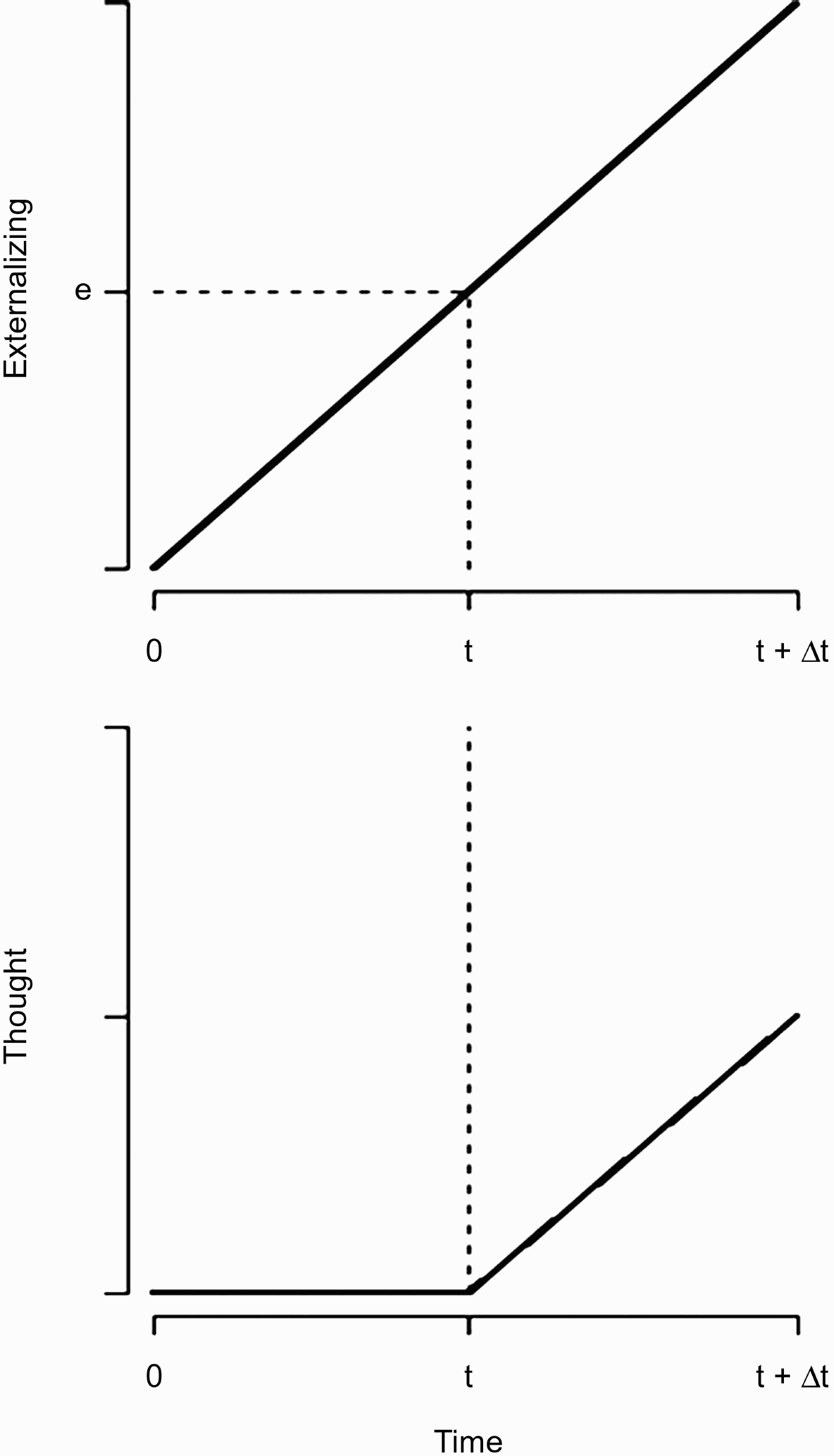
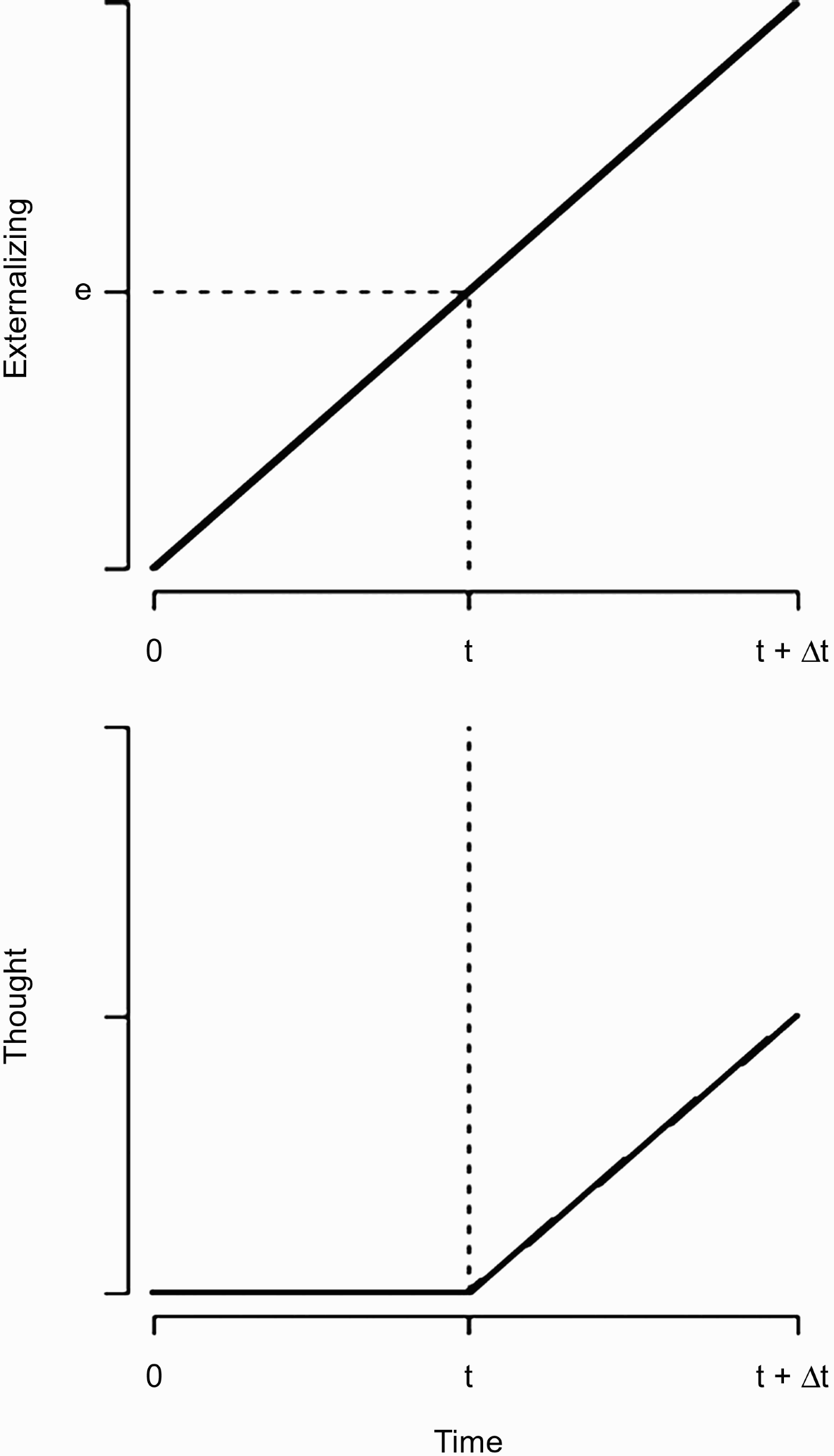
A model of a cascade consistent with the above definition is depicted in Figure 1. The figure shows the graph of a growth curve of externalizing problems and of thought problems. In this scenario externalizing problems are the predictor and thought problems the response. The upper graph depicts a linearly increasing externalizing growth curve that reaches a threshold level e, at time t, represented by the horizontal and vertical dashed lines, respectively. The thought problems growth curve is flat up to time t (i.e., dormant), but is activated at that time by the threshold level of externalizing problems and begins to increase. The terminus is t + Δt with the elevated level of externalizing problems accompanied by an elevated level of thought problems. One can imagine the converse situation in which externalizing never reaches the threshold e, so that thought problems do not increase for the duration.
A conceptual example of a cascade. The upper graph depicts a linearly increasing externalizing growth curve that reaches a threshold level e at time t, represented by the horizontal and vertical dashed lines, respectively. The terminus is t + Δt.
Given the definitions of continuity and cascade, it seems important to model changes in the level of the variables over time. In longitudinal studies it is not always possible to model the level because this requires that the same instrument is administered repeatedly (Long, Harring, Brekke, Test, & Greenberg, Reference Long, Harring, Brekke, Test and Greenberg2007). Developmental appropriateness dictates that measures must sometimes be exchanged. One advantage of the current study is that the same measure was used over the time span considered (early childhood to late adolescence).
In addition to examining change in level, lagged correlations may also be important. A lagged correlation in this context means that the predictor is measured at an earlier time point than the response. This correlation may be useful when one wants to predict the response at the terminus. Figure 1 can be used to illustrate this assuming the growth curves are for an individual. Let t + Δt be the terminus at which thought problems are measured and let time t be the time point at which externalizing problems are measured. One can also imagine a growth curve for externalizing problems in which the threshold is never reached yielding a low value (or zero value) of thought problems. Considering several individuals with a variety of externalizing values below and above the threshold at time t, a positive correlation with thought problems at time t + Δt is evidence of a cascade. In predicting the response at the terminus, the predictor can also be an average over a particular time span. For example, we might sum the values of externalizing problems for the time point less than or equal to t, and then use this composite to predict thought problems at time t + Δt. Thus, the predictor can be a cumulative index of level.
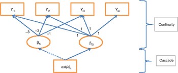
Continuity and cascades may be examined within the context of growth curve modeling. A conceptual example is provided in Figure 2 that depicts linear growth over four time points for one of the clinical groups. In the analysis to be described below, we use interaction terms to fit models similar to Figure 2 for each clinical group. The continuity (discontinuity) portion is a growth curve model for an individual with Yij being the response variable score, for example, thought problems, for the ith participant (i = 1, … , N) at the jth time point (j = 1, … , 4), and β0i and β1i are unobserved individual-specific effects. The linear slope for the individual growth curve is β1i and the coding of the path coefficients (−3, −2, 1, 0) sets the intercept, β0i, to be the status at the terminus. The expected values of β0i and β1i, β0 and β1, respectively, are the fixed effects defining the group-level growth curve. The investigation of continuity involves linear and nonlinear growth curves, the latter being at least quadratic or cubic polynomials, which can be specified by including additional unobserved variables with path coefficients that are power transformations of the linear coefficients.
Continuity and cascade within the growth curve model. [A color version of this figure can be viewed online at journals.cambridge.org/dpp]

The cascade portion involves the regression of β0i and β1i on a cumulative index of the predictor, for example, cumulative externalizing problems ext(c)i. The index is a running average that represents the accumulation of the variable up to and including the cth time point. Based on Figure 2 that depicts four waves of measurement, we have ext(1)i, the externalizing score at the earliest age, ext(2)i, the average of the two earliest externalizing scores, ext(3), the average of the three earliest externalizing scores, and ext(0)i representing the omission of externalizing scores altogether. Based on Figure 1, there are two types of cascade effects: one for the growth curve represented by ext(c)i → β1i, and the other for the terminus represented by ext(c)i → β0i. In Figure 1, the ext(c)i → β1i is dashed, as this path was not examined in our analysis because of a small sample size.
Research Addressing Continuity and Cascade Models
Despite the growing body of research confirming that O-BD are at risk for a range of behavioral and emotional problems, limited research has been conducted to evaluate patterns of continuity or discontinuity that characterize O-BD. Furthermore, developmental cascades have yet to be studied in this risk group, requiring us to draw on the small body of work that identifies systematic shifts in problems over time. In several studies, problems in O-BD would be best described as having a discontinuous developmental trajectory. Some have noted good early functioning followed by an abrupt onset of problems later in childhood or adolescence (Duffy et al., Reference Duffy, Alda, Kutcher, Cavazzoni, Robertson and Grof2002). Other results have also suggested lack of continuity. Hammen, Burge, Burney, and Adrian (Reference Hammen, Burge, Burney and Adrian1990) reported that O-BD had few chronic, recurrent, or new episodes on psychiatric diagnoses over a 1- to 3-year follow-up. In their longitudinal study that included one follow-up 3 to 7 years after the initial assessment, LaRoche et al. (Reference LaRoche, Sheiner, Lester, Benierakis, Marrache and Engelsmann1987) found that 24% of the adolescents (on average, age 16 years, ranging from 8 to 25 years) carried a diagnosis. Although evidence of some continuity of affective traits across time was documented, no continuity of exact problems existed, and only 3 of the 37 adolescents received a diagnosis at both time points. Hillegers et al. (Reference Hillegers, Reichart, Wals, Verhulst, Ormel and Nolen2005) reported on the 5-year prospective outcomes of O-BD, with overall stability of problems not evident.
Some have suggested systematic changes in problems occur at different points in development. For example, Carlson and Weintraub (Reference Carlson and Weintraub1993) found that attentional and behavioral problems during early childhood were associated with a broad range of problems in adulthood, including affective illnesses. Akiskal, Downs, Jordon, and Watson (Reference Akiskal, Downs, Jordon and Watson1985) reported that for younger O-BD, comorbid diagnoses are often mood problems as well as ADHD and Disruptive Behavioral Disorders. For adolescents and young adults, pathology is mostly accounted for by primary mood disorders. In summary, although some evidence indicates that O-BD may exhibit persistent problems, there is other evidence to suggest that risk pathways for O-BD may be characterized by a fluctuating course. Duffy et al. (Reference Duffy, Alda, Kutcher, Cavazzoni, Robertson and Grof2002) concluded that variability between studies likely reflects the approaches used because research to date has largely failed to carefully characterize developmental fluctuations in symptom presentation.
There is a paucity of research that relies on repeated prospective longitudinal research with O-BD. Radke-Yarrow and colleagues (Radke-Yarrow & Klimes-Dougan, Reference Radke-Yarrow, Klimes-Dougan, Luthar, Burack, Cicchetti and Weisz1997, Reference Radke-Yarrow, Klimes-Dougan, Goodman and Gotlib2002; Radke-Yarrow et al., Reference Radke-Yarrow, Martinez, Mayfield and Ronsaville1998) represent one of the few efforts that have repeatedly assessed risk variables for O-BD, O-UNI, and O-WELL over narrowly defined periods of development using a prospective longitudinal design spanning more than a decade. Group differences were not always found for offspring during any single assessment wave. Cumulative problems were evaluated within individuals using survival analyses. O-BD and O-UNI showed higher levels of clinically significant problems than O-WELL. That is, for the three groups, 73%, 76%, and 37% exhibited depressive problems; 64%, 79%, and 43% exhibited anxiety problems; and 54%, 71%, and 20% exhibited oppositional–disruptive problems, respectively. An important next step is to clarify the problem course of O-BD by examining developmental continuities and cascades.
Building on this past research, the first aim of this study was to evaluate if O-BD and O-UNI showed different continuity/discontinuity profiles from childhood through adolescence from the O-WELL for the three problems assessed, externalizing, internalizing, and thought problems. A second aim was to evaluate support for a developmental cascade. We hypothesize that over time the persistence of self-regulatory deficits, as exhibited by externalizing problems, will portend disruptions in internalizing problems and thought processes. This should be manifested by a statistically significant prediction of the terminus of thought disorders and internalizing problems by an earlier accumulation of externalizing problems. We predict that the developmental cascade will differ for O-BD and O-UNI and O-WELL mothers. To address these aims, secondary analysis of the NIMH Childrearing Study was considered, with participants spanning from early childhood through late adolescence (e.g., Radke-Yarrow et al., Reference Radke-Yarrow, Martinez, Mayfield and Ronsaville1998).
Method
Sample
The 94 families that were selected to participate in this study were part of a longitudinal investigation of offspring of depressed and well mothers, resulting in 22 O-BD, 42 O-UNI, and 30 O-WELL. Of the offspring, 40% were males. For the purpose of this study the older child participants (approximately two-thirds were first born) from each family were selected because they span the age from early childhood through mid to late adolescence when internalizing and thought problems are likely to manifest. Other studies published with this sample typically have also included the younger cohort; the focus of this study was on the older sibling cohort only.
Demographic characteristics
Families were predominantly middle class to upper middle class; the average Hollingshead socioeconomic status (Hollingshead, Reference Hollingshead1975) score was 51.08 (SD = 14.84). Most parents were college educated (75% of the mothers). Ninety-four percent of the families were intact (70% remained intact). The sample was 86% Caucasian, 11% African American, 2% Asian American, and 1% Hispanic.
Recruitment
The families were a volunteer sample. They responded to announcements in local news sources (e.g., newspaper, day care centers). The families were screened via telephone on the mother's apparent mental illness status, the ages of the children, the mother's caregiving responsibilities (e.g., whether they were primary caretakers), and the composition of the family (e.g., parents living in the home). Families that met the screening criteria were then assessed to establish their eligibility for this study. Of the families that met the initial criteria for participation in the longitudinal study (N = 126; initially mothers with minor depression were also included), attrition rates were 17%, 12%, and 9% for the well, bipolar, and unipolar depressed mothers, respectively. Radke-Yarrow et al. (Reference Radke-Yarrow, Martinez, Mayfield and Ronsaville1998) contains a more complete account of recruitment, sample description, and attrition.
Procedure
The families were seen at four periods of the children's development. At assessment Waves 1, 2, 3, and 4, the mean ages were, 6.36 (SD = 1.06) years, 9.27 (SD = 1.24), 13.03 (SD = 1.42), and 17.67 years (SD = 1.94, respectively. During these four periods, comprehensive assessments were conducted on the parents' and children's psychiatric status, the children's psychosocial functioning, and the families' functioning. The CBCL (Achenbach, Reference Achenbach1991) was administered at each assessment. For the statistical analysis described below, the age at measurement was used rather than the wave of measurement.
Parental diagnoses and functioning
Mothers were administered the Schedule for Affective Disorders and Schizophrenia: Lifetime Version (SADS-L; Spitzer & Endicott, Reference Spitzer and Endicott1977). The interviews were conducted by a psychiatric nurse trained by a staff member from the New York Psychiatric Institute. One hundred percent agreement was achieved on 10 interviews coded independently by the nurse and the New York Psychiatric Institute staff. Mothers were eligible if they met the research diagnostic criteria (Spitzer, Endicott, & Robins, Reference Spitzer, Endicott and Robins1978) for major depressive disorder, BD (bipolar I or II), or minor depression (not included here), or were without past or current psychiatric disorder. If the mother was eligible, the SADS-L interview was also administered to the father. Spouses of the depressed mothers were either without psychiatric disorder or suffered from depression or anxiety. For the well families, both parents had to be without current or past psychiatric disorder.
Six years into the study, mothers were rediagnosed using the Structured Clinical Interview for DSM-III-R (SCID; Spitzer et al., Reference Spitzer, Endicott and Robins1978) and the Interval SADS. Nine mothers' diagnoses were changed (seven of which changed in the type of depression manifest). The diagnosis used in this study is the mother's adjusted “lifetime” diagnosis. Fathers were also rediagnosed using the Interval SADS. Two-thirds of the husbands of the depressed mothers had at least one psychiatric disorder (mood disorder, anxiety disorder, and/or substance abuse disorder). From the initial diagnostic interview, clinicians rated the mothers on the Global Assessment Scale (Endicott, Spitzer, Fleiss, & Cohen, Reference Endicott, Spitzer, Fleiss and Cohen1976). The average Global Assessment Scale score for the depressed mothers was 43.22 (SD = 19.77) at a level of “serious symptomatology or impairment in functioning that most clinicians would think obviously requires treatment or attention” (Endicott et al., Reference Endicott, Spitzer, Fleiss and Cohen1976, p. 176).
Child emotional and behavioral problems
Measures of children's internalizing and externalizing problems were based on raw scores from the broadband internalizing and externalizing scales, and the thought problems subscale of the CBCL (Achenbach, Reference Achenbach1991). CBCL validity and reliability estimates as reported in the test manual are good for the broadband scales. The CBCL was completed by the primary caretaker (the biological mother for 92% of the children during all periods). All analyses used individual assessment.
Statistical analysis
The statistical analysis involved fitting continuity/cascade models similar to the one depicted in Figure 2 for each risk group using interaction terms as described in a moment. The continuity analysis consisted of fitting linear and nonlinear growth curve models for thought problems, externalizing problems, and internalizing problems. The cascade analysis consisted of using a cumulative index of externalizing problems, ext(c)i, as a predictor of terminal status for thought problems and internalizing problems separately. The cumulative index was computed by averaging waves of externalizing scores. The form of the growth curve for the cascade analysis was determined from the continuity analysis. For example, if a linear curve was sufficient in the continuity analysis, then this was also used in the cascade analysis.
The ext(c)i → β1i path indicated by a dotted line in Figure 2 was not estimated, meaning the cumulative externalizing index was not used to predict the growth curves. The reason was that nonlinear trends coupled with a limited sample size (N = 94) constituted an analysis in which relatively high-parameter models would be estimated based on limited information. Allowing nonlinear trends but predicting only terminal status provided for a reasonable number of parameters to be estimated given the sample size.
An important analysis issue was that each response variables had a positively skewed distribution often accompanied by a mode of zero. Because the variable values were integer and could be conceptualized as counts of symptoms, a regression model with a Poisson probability distribution was used for the analysis. In order to account for the dependency because of repeated measures, a generalized linear mixed effects regression (GLMER) model with a natural log link was used. The GLMER for longitudinal data can be depicted as a two-level hierarchical model with the first level representing the individual-specific growth curve and the second level representing group-level effects as shown below.
GLMER models were estimated using maximum likelihood methods. All analyses were performed in R using the glmer() function of the lme4 package with the family = poisson option (Bates, Reference Bates2005). Maximum likelihood methods provide unbiased parameter estimates under the assumption that the missing data mechanism is at least missing at random.
As outlined in the two sections below, there were a number of hypothesized alternative models. For the cascade analysis many of these models were not nested and could not be tested with traditional approaches such as the likelihood ratio test. Thus, a multimodel approach was used that focused on relative model fit rather than statistical tests (Anderson, Reference Anderson2008; Burnham & Anderson, 2002, Reference Burnham and Anderson2004). In the multimodel approach the best fitting model is often considered for adoption, but the relative fit of other models is made explicit. This approach provides an indication of the model uncertainty usually neglected in null hypothesis testing (Chatfield, Reference Chatfield1995). Statistics such as z values can be used as indicators of effect sizes, but these statistics are not used to select models.
Because the sample size was not large, fit was evaluated with a version of the Akaike information criterion (AIC; Akaike, Reference Akaike, Atkinson and Fienberg1985) corrected for small samples (AICC; Hurvich & Tsai, Reference Hurvich and Tsai1989). The AIC (and AICC) is based on information-theoretical principles and is an estimate of the distance of a sample-fitted approximating model to the “full reality” that generated the data (Anderson, Reference Anderson2008, chap. 4). The AICC is computed using the maximized likelihood and a penalty term for the number of parameters and the total number of data points,

where −2LL is −2 times the log likelihood, K is the total number of parameters, ni is the number of observed time points for the ith participant, and ∑ini is the total number of data points with ∑ini = 323 in the analysis presented below.
When a group of models is fit to the same data, the one with the smallest AICC value is the best fitting but other models may have nearly equivalent fit. In order to quantify the relative fit among several models one can compute the model distance measure, Δp. Suppose the AICC value of the pth model is denoted as AICCp. Then,

where AICCmin is the smallest AICC value among the models considered. The best fitting model has Δp = 0 and worse fitting models have Δp > 0. A further refinement is to scale Δp to be a probability (in the interval of 0 to 1). The scaling formula is
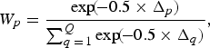
where Wp is known as the weight of evidence for the pth model and ∑q denotes summation over all the models in the set. It can be shown that the sum of the Wp is 1 and the model with the largest weight is the best fitting (Burnham & Anderson, Reference Burnham and Anderson2004). If a model accounts for a high proportion of total probability (e.g., 0.80), then it is a good candidate for adoption. When a subgroup of models accounts for a substantial portion of the total probability, then multiple candidates might be considered.
A final metric helpful for comparing relative fit is the evidence ratio (Ep), which is the ratio of the Wp for the best fitting model to that of all other models. That is,
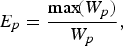
where max(Wp) denotes the weight of evidence for the best fitting model of the set. The best fitting model has Ep = 1, and for the other models, Ep > 1. Here, Ep indicates how many times better fitting the best model is relative to the pth model. Because the Wp are probabilities, Ep is the odds against the pth model being the best fitting under replication (Anderson, Reference Anderson2008, chap. 4). Thus, a large value of Ep argues against the plausibility of the pth model.
In the analyses below we focus on the best fitting model but present the fits for all of the models in a set. As shown in the results, the top three or four best fitting models accounted for the majority of probability in all cases. To provide an indication of effect size for specific effects (e.g., group intercept differences), parameter estimate/standard error (z) values were compared. Because of the large number of parameters in some models (e.g., 15), parameter estimates are not presented and the focus is on global model fit. Parameter estimates for all models are available from the authors.
Continuity analysis
The continuity analysis consisted of fitting linear and nonlinear growth curves allowing differences among the risk groups. Each model had Intercept × Group interactions and Trajectory × Group interactions. The most complex growth curve considered was the cubic polynomial. The GLMER cubic polynomial model can be depicted as a two-level model. Suppose Yij is the response score of the ith participant (i = 1, … , N) at the jth time point (j = 1, … , ni), and conditional on random effects, Yij has a Poisson distribution with mean λij. Then the cubic GLMER for count data is the following:





where Equation 1 is the individual-level model and Equations 2a–2d constitute the group-level models. Max is the maximum age among all the participants so that β0i represents an individual's level at the terminus (oldest observed age). Because of sparse data at the last time point for internalizing problems (age 21.5), the max value was set to 20 for all variables in all analyses. In the group-level equations (Equations 2a–2d), bpi is a dummy code that takes the value of 1 if a participant is in the O-BD group and 0 otherwise, and unii is a dummy code that takes the value of 1 for O-UNI and 0 otherwise. Here, βk is a fixed effect and bki is a random effect. Two random effects are typically sufficient for GLMER (Long, Loeber, & Farrington, Reference Long, Loeber and Farrington2009), and that was the number used in all analyses. The random effects are assumed to have a joint-normal distribution with zero means and variance–covariance matrix ∑.
The set of fixed effects associated with the dummy codes in Equations 2b–2d represent group differences for the growth curves. For example, in Equation 2a, β4 represents intercept differences between the O-BD and O-WELL groups and β8 represents intercept differences between O-UNI and O-WELL. When further clarification was needed, O-BD and O-UNI group differences were also estimated.
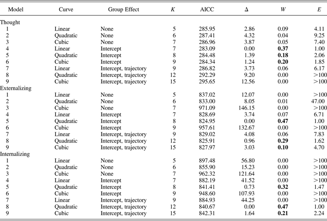
The two-level model of Equations 1 and 2 was the most complex model considered. Less complex models had either a lower order polynomial growth curve or group effects only for individual intercepts (β0i). This resulted in nine hypothesized models for each variable. The nine models are classified in Table 1 by the type of growth curve (linear, quadratic, cubic) and type of group effect (none, intercept, trajectory).
Continuity analysis results
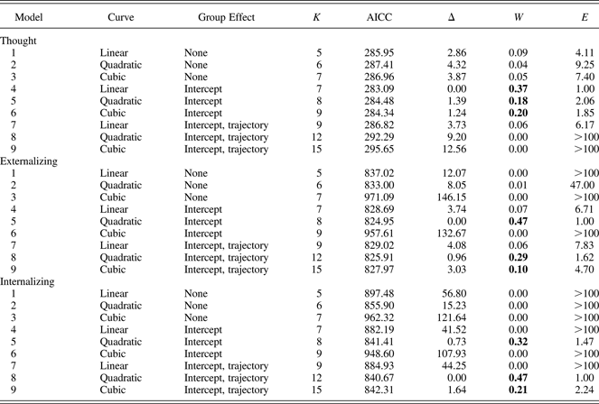
Note: K, number of parameters; AICC, Akaike information criterion corrected; Δ, scaled AICC; W, weight of evidence; E, evidence ratio. The top three values for each variable are in bold.
Cascade analysis
The cascade analysis used the cumulative index of externalizing problems as a predictor of the terminus of thought problems and internalizing problems (see Figure 2). The growth curve portions were based on models suggested from the continuity analysis (see the results below). Each subject had four waves of data, although the age at each wave was not constant among the subjects. There were four externalizing cumulative index scores that were computed by averaging externalizing problems scores for the waves: ext(c)i, c = 0, 1, 2, 3. The first, ext(0)i, constituted not using externalizing at all,
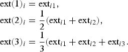
Each cumulative score was used as a predictor separately in the model.
One of the research hypotheses was that the strength and/or nature of the cascade might vary by risk group. Therefore, risk group interaction terms were an integral part of the cascade models. Conceptually, this was similar to fitting the path model of Figure 2 (omitting the dotted path) separately for each risk group with the caveat that the growth curve could be nonlinear depending on the results of the continuity analysis.
The most complex model considered was a quadratic polynomial with a group terminus effect and group by ext(c)i interaction. The most complex model can be written in hierarchical form as

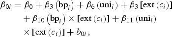


where β10 and β11 are the Group × Cumulative Index interactions and all other terms are as previously defined.
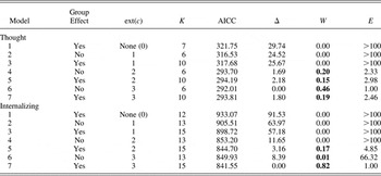
Equations 3 and 4 constitute the most complex model but simpler models were also considered by omitting ext(c)i and its interaction terms as predictors of intercepts from Equation 4a. We considered the combination of cascade group effects (none or intercept) and accumulation (c = 0, 1, 2, 3) to define seven alternative models for each cascade analysis as shown in Table 2.
Cascade analysis results

Note: ext(c), cumulative index; K, number of parameters; AICC, Akaike information criterion corrected; Δ, scaled AICC; W, weight of evidence; E, evidence ratio. The best fitting models are in bold.
Results
Continuity results
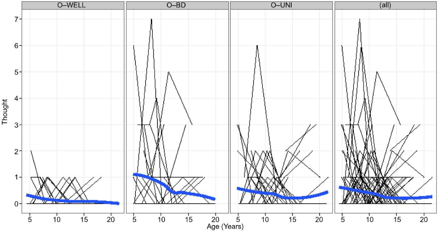
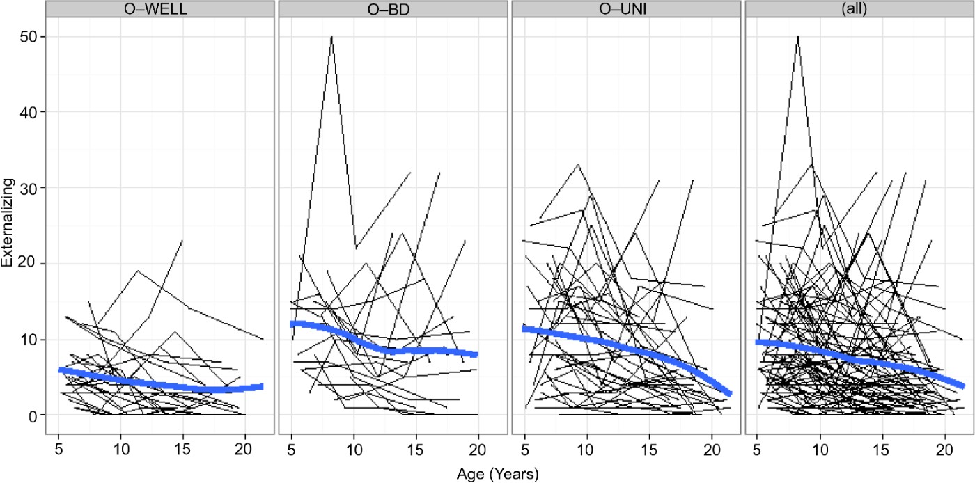
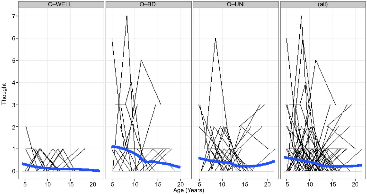
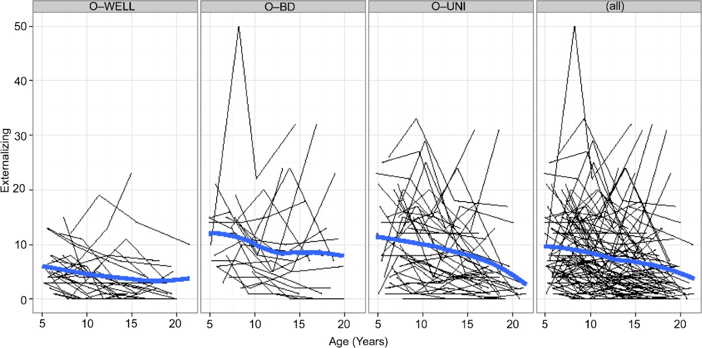
Graphs of growth curves for thought problems, externalizing problems, and internalizing problems are shown in Figure 3, Figure 4, and Figure 5, respectively. The narrow lines are observed individual growth curves and the thick lines are smoothed curves based on local polynomial fitting (Cleveland, Grosse, & Shyu, Reference Cleveland, Grosse, Shyu, Chambers and Hastie1992). The four panels represent the O-WELL, O-BD, O-UNI, and all groups combined (all). The figures depict the raw counts, whereas GLMER models the log of the counts. This means the smooth curves in the figure and those based on GLMER are monotonically related. For example, a linear curve under the log link will be nonlinear but monotonic in the raw count metric. The count curves in the figures were sufficiently similar to the curves for the log means, so only the former are presented.
Individual growth curves (thin lines) and smoothed curves (thick lines) for thought problems by risk group. [A color version of this figure can be viewed online at journals.cambridge.org/dpp]
Individual growth curves (thin lines) and smoothed curves (thick lines) for externalizing problems by risk group. [A color version of this figure can be viewed online at journals.cambridge.org/dpp]
Individual growth curves (thin lines) and smoothed curves (thick lines) for internalizing problems by risk group. [A color version of this figure can be viewed online at journals.cambridge.org/dpp]

For thought problems, the smoothed curves show a tendency to decrease over time with the exception of a slight late increase in the O-UNI curve. The curves for the risk groups appear to have more “wiggle” than the curve for O-WELL. The smoothed curves for externalizing problems also showed a tendency to decrease over time with a slight nonlinear trend perceptible in all three groups. For internalizing problems, the smoothed curves were nonlinear with the O-BD and O-UNI curves having concave-down trends and the O-WELL curve having a near-horizontal curve with two shallow bends. The graphs provide preliminary evidence that the groups might differ in terms of continuity.
Thought problems
The results of the continuity analysis are shown in Table 1. All statistical results pertain to the log metric of the GLMER model (see Equation 1). The last four columns show the values of K, AICC, Δ, W, and E. The top three values of weight of evidence (W) for each variable are in boldface and account for the majority of the probability. For thought problems, the best fitting model was Model 4 (W 4 = 0.37), which had a linear growth curve and group intercept differences. The next two best fitting models (W 6 = 0.20, W 5 = 0.18) had nonlinear growth curves and group intercept differences Model 4 was approximately twice as good fitting as Model 6 (E 6 = 1.85) and Model 5 (E 5 = 2.06).
Parameter estimates (not presented) indicated that the O-BD group had the highest intercept value estimate, followed by the O-UNI group and then the O-WELL group. The intercept difference between the O-BD and the O-WELL groups was the largest (z = 2.69), followed by the difference between the O-UNI and O-BD groups (z = 1.69). An additional comparison (not presented) showed the intercept difference between the O-BD and O-UNI groups was smaller than the other two group differences (z = 1.37).
In summary, the best fitting model had a linear growth curve for all three groups with the O-BD and O-UNI groups having a higher intercept than the O-WELL group.
Externalizing problems
For externalizing problems, the best fitting model was Model 5 (W 5 = 0.47), which had a quadratic growth curve and a group effect for intercept. The next two best fitting models included group effects for intercepts and trajectories (W 8 = 0.29, W 9 = 0.10). Model 5 was a little less than twice as good fitting as Model 8 (E 8 = 1.62) and almost five times as good fitting as Model 9 (E 9 = 4.70).
The parameter estimates for the best fitting model (not shown) revealed a negative value for the quadratic curve indicating a concave-down shape (see Figure 2). The two depression groups, O-BD and O-UNI, had nearly identical intercept values and were greater than the O-WELL group. The intercept difference between O-UNI and O-WELL had the highest z value (z = 3.37) but the difference between O-BD and O-WELL also had a high z value (z = 3.07). An additional comparison showed the difference between O-BD and O-UNI was relatively small (z = 0.21).
In summary, the best fitting model had a quadratic concave-down shape for all groups with the O-BD and O-UNI groups having nearly identical intercepts that were higher than the O-WELL group.
Internalizing problems
The results for internalizing problems show the best fitting model was Model 8 (W 8 = 0.47), which had a quadratic growth curve with group differences for both intercepts and trajectories. The next best fitting model omitted the group trajectory difference (W 5 = 0.32), and the third best fitting model had a cubic growth curve and both group intercept and trajectory differences (W 9 = 0.21). Model 8 was approximately 1.5 times as good fitting as Model 5 (E 5 = 1.47) and more than twice as good fitting as Model 9 (E 9 = 2.24).
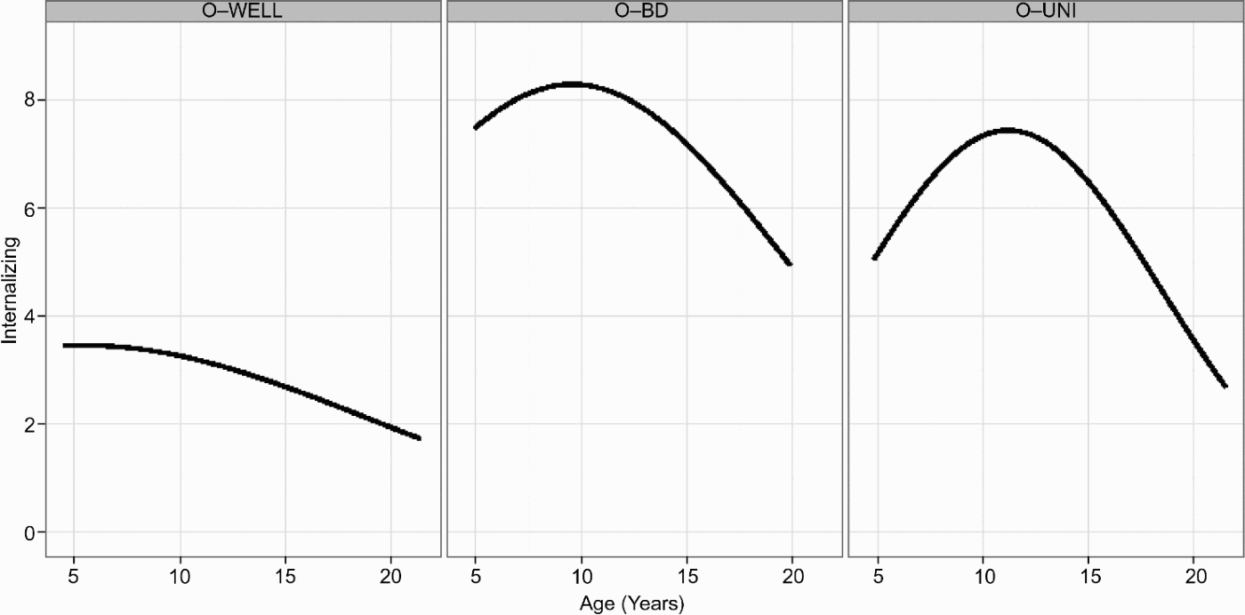
Parameter estimates of the best fitting model (not presented) revealed that all groups had a negative quadratic coefficient indicating a concave-down pattern (see Figure 5). The O-UNI group had a negative quadratic value that was substantially larger than the O-WELL group (z = −2.53). The O-BD group had a similar negative quadratic value as the O-WELL group (z = −0.83), which was close to zero, that is, close to a linear pattern. As for intercept differences, the O-BD intercept value was the highest, followed by O-UNI and then O-WELL. The intercept difference between O-BD and O-WELL was not especially large (z = 1.77), and the difference between O-UNI and O-WELL was even smaller (z = 0.60), as was the difference between O-BD and O-UNI (z = –0.91).
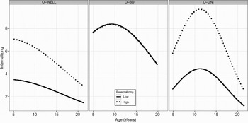
To better understand the group differences, the prediction curves based on the fitted Model 8 are shown in Figure 6. The log results were backtransformed using the antilog (ex) to produce the curves in Figure 6. The O-WELL and O-BD trends were nearly linear in the log metric but are nonlinear in Figure 6 because of the backtransformation to the count metric. The curve for the O-WELL group is monotonically decreasing, whereas the curve for the other two groups initially increases before decreasing. That is, the O-BD and O-UNI groups show greater curve complexity than the O-WELL group, although only the effect for O-UNI is statistically reliable.
Predicted growth curves for internalizing problems by risk groups based on the continuity analysis.
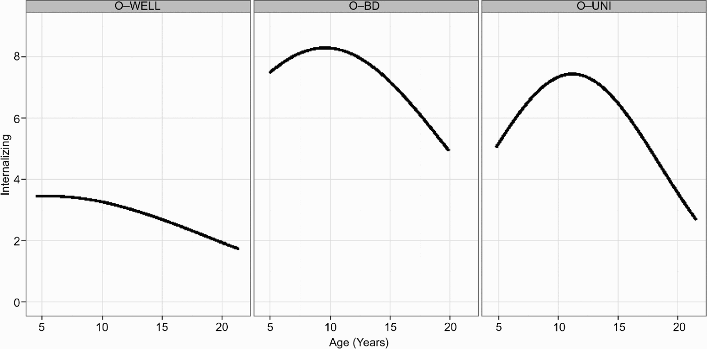
In summary, the best fitting model had group differences in trajectory, with the O-UNI group having a quadratic concave-down pattern and the other two groups having a nearly linear pattern (in the log metric).
Cascade results
The cascade analysis was based on the best fitting models from the continuity results, namely, Model 4 for thought problems and Model 8 for internalizing problems (see Table 1). The cascade results are shown in Table 2. For thought problems, there were four models that had substantial weights with the best fitting Model 6 (W 6 = 0.46) having a weight more than twice the size of the next best fitting Model 4 (W 4 = 0.20). The best fitting model had no group differences but did show a cascade effect for the terminus (age 20) with the ext(3)i accumulation index. The second best fitting model (Model 4) was similar to the best fitting but had ext(2)i as the accumulation index. The third best fitting model (Model 7, W 7 = 0.19) had group differences for the ext(3)i cascade. The fourth best fitting model (Model 5, W 5 = 0.15) also had group differences but for ext(2)i. In the best fitting model (Model 6), parameter estimates (not presented) showed that the estimated cascade coefficient, ext(2)i → β0i, was positive, indicating that those with higher externalizing problems also had higher thought problems at the terminus (and the converse).
For internalizing problems, the best fitting Model 7 had a very large weight (W 7 = 0.85) and the next best fitting Model 5 had a weight that was substantially smaller (W 5 = 0.17) and was approximately five times worse fitting (E 5 = 4.85). The third best fitting Model 6 had a weight that was almost zero (W 6 = 0.01) and was approximately 66 times worse fitting than Model 7 (E 6 = 66.32). The best fitting model (Model 7) had cascade effects of ext(3)i that varied by risk group. The second best fitting model (Model 5) was similar but had ext(2)i predicting intercepts. For the best fitting model, parameter estimates (not shown) indicated the O-WELL group had a substantial positive ext(3)i → β0i cascade coefficient (z = 2.33). The O-BD coefficient was near zero and much smaller than the O-WELL coefficient (z = −2.06). The O-UNI coefficient was approximately equal to that of O-WELL (z = 0.23).
To illustrate the cascade effect for internalizing problems, the predicted curves were computed based on the fitted Model 7. Figure 6 shows the internalizing fitted curves depicted for the first and third empirical quartiles of ext(3)i. As the figure shows, higher values of cumulative externalizing problems were associated with higher overall levels of internalizing problems for the O-WELL and the O-UNI groups. The O-BD group curves were virtually identical.
In summary, there was a cascade effect for thought problems with the ext(3)i → β0i coefficient estimate being positive and indicating that higher cumulative externalizing problems were associated with higher terminal thought problems. This effect did not vary statistically among the groups.
For internalizing problems, the ext(3)i → β0i coefficient was positive and nearly equal for the O-UNI and O-WELL groups indicating that higher cumulative externalizing problems were associated with higher terminal internalizing problems. The O-BD group had a substantially smaller and near-zero coefficient indicating a negligible relationship between cumulative externalizing problems and terminal internalizing problems.
Post hoc cascade results
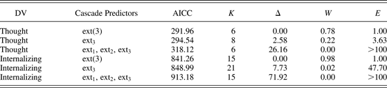
To provide additional validity regarding the cumulative effect of externalizing problems in the cascade analysis, we compared the best fitting models of Table 2 with two additional models. First, we wanted to consider the possibility that ext(3)i was an effective predictor because it was constructed partly of externalizing problems closest in time to the terminus problems that it was predicting, ext3i. To examine this, externalizing problems of the third wave of measurement for each subject were used as a predictor of outcome problems. Second, we wanted to consider the possibility that the three waves of externalizing problems did not need to be accumulated but that the single predictors, ext1i, ext2i, ext3i, would predict equally as well. To examine this question the first three waves of externalizing problems replaced the cumulative index in the best fitting models.
The results of the post hoc model comparisons are shown in Table 3. For thought problems, the cumulative index model was the best fitting and the model including just ext3i was almost 4 times worse. The model with the single predictors had extremely poor relative fit. Similarly, for internalizing problems the cumulative model was the best fitting and the model including just ext3i was almost 48 times worse. The model with the single predictors had even worse relative fit.
Post hoc cascade analysis results
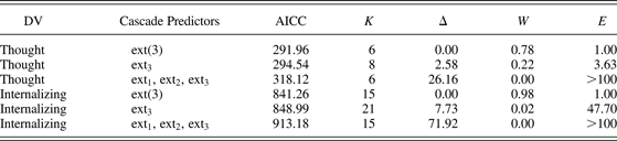
Note: ext(3) = (ext1 + ext2 + ext3)/3; AICC, Akaike information criterion corrected; K, number of parameters; Δ, scaled AICC; W, weight of evidence; E, evidence ratio.
Discussion
This study examined patterns of risk associated with being born to and raised by a mother with bipolar depression. Longitudinal approaches provide a potential means by which the transactional and progressive associations of problem behavior can be identified (e.g., Cicchetti & Rogosch, Reference Cicchetti and Rogosch2002; Masten & Curtis, Reference Masten and Curtis2000; Masten et al., Reference Masten, Roisman, Long, Burt, Obradovic and Riley2005; Masten, Long, Kuo, McCormick, & Desjardins, Reference Masten, Long, Kuo, McCormick and Desjardins2009; Rutter & Sroufe, Reference Rutter and Soroufe2000). Some have advocated for the evaluation of developmental cascades, an approach that accounts or controls for preexisting and ongoing concurrent associations.
The data used in this study provided numerous advantages for considering developmental continuity and cascades. A long-term longitudinal design was employed spanning more than a decade. Well-validated constructs were used to assess risk status, including broadband internalizing and externalizing scales to measure these classes of risk previously identified in offspring of depressed parents. We also directed our efforts to understanding symptoms associated with psychosis. The availability of repeated assessments from the same scales allowed us to employ advanced data analytical techniques that apply growth curve models to evaluate developmental progression. Age at each of the four assessments was used in the model to account for developmental shifts that occur in adolescence and early adulthood. Because statistical models are not always made clear in the extent literature, we attempted to provide detailed definitions of continuity/discontinuity and cascades, which were illustrated in the data analysis. This study not only serves to advance our understanding of the risks associated with a family history of BD but also provides a novel approach to examining developmental cascades.
The first series of questions we addressed with growth curve models pertained to continuity of a specific problem. Here we considered patterns across time separately for externalizing, internalizing, and thought problems. For each response variable, Table 1 indicates that all the best fitting models showed an intercept difference among the groups. Consistent with less precise previously employed methodologies that assessed trends across time (e.g., Radke-Yarrow & Klimes-Dougan, Reference Radke-Yarrow, Klimes-Dougan, Goodman and Gotlib2002), all three problems assessed were more severe in offspring of bipolar and unipolar parents, and few problems were noted in offspring of well families. Although as a whole externalizing and internalizing problems in the high-risk groups were consistent with subclinical impairment, very low levels of thought problems were identified across all groups.
Discontinuity was evident with internalizing problems as the growth curve for the high-risk groups was more complex than for the low risk group (see Figure 5). In particular, offspring of mothers with unipolar depression had a growth curve with the greatest degree of concavity (see Figure 6). Although this pattern noted in offspring of unipolar mothers may be attributed to a fluctuating course, it is also possible that a systematic pattern emerges for the offspring of unipolar mothers, perhaps showing a pattern of internalizing problems that peak in late childhood.
There was only tentative evidence of discontinuity between groups for externalizing and thought problems. Nevertheless, these complex progressions in the risk groups seem to indicate a highly variable course across development. Variability in results at any one assessment may yield insufficient evidence for predicting outcomes. That is, one assessment may be associated with the outcome quite differently than another assessment point of the same behavior. A nonlinear growth curve can make it difficult to use any cross-section to predict to a terminal point of another variable. In turn, it may be difficult for mental health professionals to establish a sound prognosis of the problem trajectory or determine when and how to intervene. The second set of results and the post hoc analysis provide evidence for important developmental cascades. As noted previously, a convincing argument for cascades is bolstered when externalizing problems accumulate in development to a “tipping point.” The results indicate that an earlier accumulation of externalizing problems was a statistically reliable predictor of thought disorders and internalizing problems at the terminus of 20 years (see Table 2). The models in which externalizing problems were accumulated over a longer span, that is, with ext(3), had a better fit than models with shorter spans, that is, with ext(2) or ext(1). Furthermore, the post hoc analysis supports the idea that it is the accumulation that is important in prediction rather than proximity to the terminus, or the fact that multiple earlier cross-sectional (noncumulative) measurements were collected. These finding are consistent with the cascade hypothesis as illustrated in Figure 1. Finally, the cascade findings provide some tentative support for differential cascades for offspring of unipolar and bipolar mothers.
The first cascade that we assessed pertains to the cascade of externalizing problems to thought problems. As predicted, the results suggest that cumulative impaired self-regulation, as indexed by elevated externalizing scores, may portend delusional or psychotic processes in adolescents. The results of this study failed to fully support the prediction that this cascade would more specifically characterize offspring of bipolar parents. That is, the two best fitting models for thought problems that accounted for the majority of the probability failed to support the group specificity of this cascade (see Table 2, Models 6 and 4). However, the third and fourth best fitting models (see Table 2, Models 7 and 5) suggest that there might be a group effect, as the O-BD group had the largest positive relationship. Although definitive statements are not possible given the model uncertainty, the results imply that the cascade effect might vary by group. Further research using a larger sample size is desirable.
It is important to clarify the nature of the thought problems assessed. With only a few exceptions, the level of thought problems reported in the context of this study was well within the normal range. As evident in Figure 3, most children showed no evidence of thought problems and there were only two cases in which thought problems were reportedly within the clinical range (both O-BD). More thought problems were reported when children were young, and relatively fewer symptoms were reported during adolescence. Cumulatively over the four assessments at least one symptom of thought problems was reported for 41% of the O-BD, 31% of the O-UNI, and 10% of the O-WELL. Although it is possible that these identified problems reflect the capacity for creative, original or divergent thinking, it is also possible that thought problems precede or are concurrent with significant impairment. Duffy et al (Reference Duffy, Alda, Crawford, Milin and Grof2007) identified offspring of bipolar parents with neurodevelopmental disorders (defined to include ADHD, Cluster A traits, and psychosis not otherwise specified). More than one-third of these identified children had developed a mood disorder at follow-up. Others have noted that it is likely that when youth exhibit delusional or psychotic thinking, they have a poor prognosis (e.g., Dunayevich & Keck, Reference Dunayevich and Keck2000). It is possible that earlier these thought problems merely reflect divergent thinking but by adolescents they represent a more entrenched psychotic process. Further research is needed to address these important questions.
Presumably, if children are exhibiting regulatory challenges early on and caretakers in their environment fail to address these needs, distortions of reality testing may persist. A previous report with this sample (Meyer et al., Reference Meyer, Carlson, Wiggs, Ronsaville, Martinez and Klimes-Dougan2006) provided some preliminary evidence that early maternal caretaking and child neurocognitive deficits negatively predicted BD in youth. Although the Meyer et al. study was not intended to evaluate a developmental cascade per se, the results of this study indicate potential ways in which one established pattern of child dysregulation may be compounded by additional neurobiological mechanisms to place the child on a specific risk trajectory.
Efforts that elaborate on the potential mechanisms by which these developmental cascades occur would be an important next step. Perhaps mother–child attachment may impact the nature of these developmental cascades. The developing regulatory capacities of the young child are dependent on the scaffolding the parents are able to provide (Kopp, Reference Kopp1982; Thompson, 1994). Depressed parents may fail to nurture these regulatory capacities in their children, leaving the child to make sense of these extremes in emotional upset. As a result, the child may inaccurately internalize their feelings, intentions, and needs, over time, generating thoughts that diverge from realistic representations of their world. A mother suffering from bipolar depression may not respond well to the self-regulatory problems in her offspring, further exacerbating a potentially dysregulated parent–child relationship.
The second cascade that we evaluated pertained to externalizing problems cascading to internalizing problems. Some have noted that depression is the most common disorder diagnosed in offspring of depressed parents (Weissman et al., Reference Weissman, Prusoff, Gammon, Merikangas, Leckman and Kidd1984) and that by late adolescence, 50% of offspring of depressed mothers will experience depression (Weissman et al., Reference Weissman, Fendrich, Warner and Wickramaratne1992). As hypothesized, group differences in cascade were found with the best fitting model indexing these differences having a very high weight of evidence (probability). Higher levels of cumulative externalizing problems were associated with higher levels of internalizing problems for the offspring of unipolar and well mothers, and the converse for lower levels was also true (see Figure 7). This association did hold for the group of bipolar offspring, but the pattern was not significant.
Predicted growth curves for internalizing problems by risk group and externalizing cumulative index based on the cascade analysis.

Although internalizing problems are consistently noted for both offspring of bipolar and unipolar parents (e.g., Radke-Yarrow, Nottelmann, Martinez, Fox, & Belmont, Reference Radke-Yarrow, Nottelmann, Martinez, Fox and Belmont1992), developmental cascades had not been assessed in this at risk population prior to this study. Consistent with our observed cascade, in a 5-year longitudinal study including offspring of unipolar mothers, Petty et al. (Reference Petty, Rosenbaum, Hirshfeld-Becker, Henin, Hubley and LaCasse2008) found that externalizing problems predicted major depressive disorders 5 years later. In contrast to our observed cascade, over a 2-year evaluation Fendrich, Warner, and Weissman (Reference Fendrich, Warner and Weissman1990) that externalizing problems in offspring of depressed mothers tended to persist and did not manifest as internalizing problems. Both family discord and parental depression appear to play an important role in predicting children's externalizing problems in their study. A number of other studies have evaluated links between early self-regulatory deficits (externalizing problems) and internalizing symptoms, albeit not in offspring of depressed parents. For example, Masten et al. (Reference Masten, Roisman, Long, Burt, Obradovic and Riley2005) in evaluating developmental cascades noted that externalizing problems in childhood appeared to undermine academic competence and subsequently showed a negative impact on internalizing problems in young adulthood. Future research should examine whether family factors such as marital or family discord as well as peer influences are associated with the developmental cascade from externalizing to internalizing problems.
Another topic for future research is to examine how developmental cascades may differ in systematic ways depending on the type of depression a parent manifests. Potential environmental and biological mechanisms may contribute uniquely to the outcomes in offspring of unipolar and bipolar parents. It is possible that the mechanism is biological and is triggered during the transition from childhood to adulthood. Although the evidence is accumulating that a diagnosis of a mood disorder is the most typical diagnostic precursor of developing bipolar depression (reviewed by Meyer & Carlson, Reference Meyer and Carlson2003), little research has investigated what problems precede depression in offspring of bipolar parents. Some would argue that the problems are cumulative and long-standing, whereas others might suggest little continuity of problems or even that the problems may appear somewhat abruptly (e.g., Akiskal et al., Reference Akiskal, Downs, Jordon and Watson1985; Hillegers et al., Reference Hillegers, Reichart, Wals, Verhulst, Ormel and Nolen2005).
Alternative interpretations of the cascade results may be considered. Accumulating disruptions in self-regulation over time may lead to problems with reality testing and internalized distress. Alternatively, the pattern found in which symptoms evolve to show changes over time may better represent heterotypic continuity. Early on, children may exhibit their thought problems by acting out, but by adolescence these problems may be more representative of delusions and hallucinations. It may also be that early forms of depression are manifest by more general forms of emotional upset. Although we have conceptualized these behavioral progressions within a developmental cascade framework, the analyses used here do not fully rule out alternative explanatory mechanisms.
There are a number of study limitations that require discussion. Because the assessments of child risk trajectories relied on maternal report, the patterns noted in the existing data may be associated with distortions in maternal perceptions as a result of the mother's disease process rather than the child's behavior. Thus, ongoing controversy exists about the validity of depressed mothers as informants on their child (e.g., Richters, Reference Richters1992; Tarullo, Richardson, Radke-Yarrow, & Martinez, Reference Tarullo, Richardson, Radke-Yarrow and Martinez1995). Although there is a wealth of data on biases associated with depression, available data about biases of mothers suffering specifically from BD are more limited. Klimes-Dougan (Reference Klimes-Dougan1998) noted that mothers with unipolar depression underestimated and bipolar mothers overestimated the symptoms relative to the child's report for suicidal symptoms. However, the findings have been mixed when comparing reports from depressed mothers and nondepressed fathers with those of their offspring (Conners et al., Reference Conners, Himmelhock, Goyette, Ulrich and Neil1979; Wals et al., Reference Wals, Hillegers, Reichart, Ormel, Nolen and Verhulst2001). Given that Farchione et al. (Reference Farchione, Birmaher, Axelson, Kalas, Monk and Ehmann2007) found modest correlations in child and parent reports of irritability and aggression, reliance on other sources of information would be a critical next step to fully understand these developmental continuities and cascades. Although multi-informant assessments are the gold standard, considerable debate continues with regard to how to resolve inconsistencies between reporters (Achenbach, Reference Achenbach1991).
Another potential limitation is that there was model uncertainty in the analysis resulting in some ambiguity. For the case of the cascade effect for internalizing problems, the results were relatively unequivocal as the best fitting model had a weight of evidence that was very large (W 7 = 0.82). In the cascade for thought problems and the continuity analysis, the best fitting model was not extreme in its superiority, meaning that other models in the set might be plausible competitors. The small sample size (N = 94) did not help matters because the resolving power of the information criteria (e.g., AICC) is limited in this case (Burnham & Anderson, Reference Burnham and Anderson2004).
Despite the model uncertainty, there appears to be evidence of a cascade for thought disorders and discontinuity for internalizing problems. For the former, the weights of evidence of the models without cumulative effects of externalizing were negligible, suggesting that accumulation is important (see Table 2). For the latter, most of the probability (.68) was accounted for by models of discontinuity with group differences (see Table 1). Thus, models that might be considered null models had very small weights of evidence in most cases, whereas models with substantive effects tended to have more substantial weights.
A number of issues pertaining to external validity should be considered in that this study sample consisted of primarily well-educated, middle to upper middle class Caucasian participants. Evaluating a homogeneous group of parents with BD may be ideal and critically important to advance our understanding of risk continuities and cascades. Considerable precision was used in identifying this sample of mothers diagnosed with BD. Nevertheless, about half of the mothers were diagnosed with bipolar I disorder (N = 10), whereas the other half were diagnosed with bipolar II disorder (N = 12). Duffy et al. (Reference Duffy, Alda, Kutcher, Cavazzoni, Robertson and Grof2002) suggested that some of the mixed findings in offspring of bipolar parents may be attributable to the heterogeneity of the types of BD diagnosed. Although broadly defined risk trajectories are sometimes more virulent in offspring of bipolar mothers (LaRoche et al., Reference LaRoche, Sheiner, Lester, Benierakis, Marrache and Engelsmann1987), some have speculated that family transmission of BD may be stronger for fathers (Kornberg et al., Reference Kornberg, Brown, Sadovnick, Remick, Keck and McElroy2000). Further research is needed to clarify potential family mechanisms. It is difficult to determine if a study examining offspring of fathers with BD would have yielded the same effect.
Potential limitations of scales used to estimate outcomes also warrant attention. Compared to the robust psychometric evidence of validity and reliability for the externalizing and internalizing problem broadband scales of the CBCL, the thought problems subscale largely lacks validation and as a rule is much less frequently endorsed. It was necessary to employ alternative assessment and analytical strategies to account for the minimal range of thought problems found in this study. Furthermore, the findings remain mixed in part because of the challenges posed in carefully attending to the developmental timing of risk assessments. Despite the advantages of using repeated assessments over time, developmental questions remain unresolved. For example, younger children may be more likely to have imaginary friends, demonstrate colorful imaginations, or hold belief systems that are not based in reality. Nevertheless, the approach advocated that emphasizes intraindividual change across development is a strength of the approach used here (e.g., Cicchetti & Rogosch, Reference Cicchetti and Rogosch2002).
Conclusion
Despite the numerous challenges in assessing cascading levels of influence associated with risk and adaptation, we have used advanced growth curve modeling techniques to investigate continuities of problems and developmental cascades. The approach we set forth here provides the reader with a potential model that can be applied to other populations to further examine risk trajectories. Our findings provide an important first step in understanding in what ways children of depressed parents exhibit continuities and discontinuities of problems over time. It also provides evidence for two developmental cascades, suggesting that when children exhibit impairments in self-regulation, over time they may develop disruptions in thinking and internalized distress. These findings enhance our understanding of the scope, breadth, and trajectory of problems exhibited by children reared by a parent who suffers from bipolar or unipolar depression. Furthermore, the results suggest that developmental trajectories in these two risk groups may be expected to differ, with self-regulatory deficits tending to cascade to thought problems for offspring of bipolar mothers and cascade to internalizing problems for offspring of mothers with major depressive disorder. Despite the risk, few resources are currently available for systematic evaluation and involvement in preventive interventions for the range of problems exhibited by offspring of bipolar parents. Adaptations of existing prevention efforts applied to offspring of mothers with depression could provide a potential first step to meet these critical needs (e.g., Garber et al., Reference Garber, Clarke, Weersing, Beardslee, Brent and Galdstonem2009).