2. THE TESTING PROBLEM

Consider a collection of time series {y_i0,…, y_iT}_{i=1,…, N} that is generated by the composite process

where f_t is an r × 1 vector of unobservable common factors, γ_i is an r × 1 vector of nonrandom factor loadings, Γ = [γ₁,…, γ_N]′ is the N × r matrix of factor loadings, and u_it is an idiosyncratic error component. The eigenvalues of the r × r matrix A are on or inside the unit circle. Specifically, we will focus on the special case A = ρI_r with |ρ| ≤ 1.³

To simplify the exposition we focus on the case without deterministic terms and short-run dynamics. The inclusion of constants, time trends, and short-run dynamics is straightforward (cf. Breitung and Das, 2005; Breitung and Pesaran, 2007) and will be briefly discussed in Section 3.

For the errors v_t and ε_it we make the following assumption.

Assumption 1. The vector ε_t = [ε_1t,…, ε_Nt]′ is independent and identically distributed (i.i.d.) with E(ε_t) = 0, E(ε_tε_t′) = Σ = diag(σ₁²,…, σ_N²), and Ψ = lim_N→∞ N⁻¹Γ′Γ a positive definite matrix. The r × 1 error vector v_t is i.i.d. with E(v_t) = 0, E(v_t v_t′) = I_r, and E(ε_t v_t′) = 0. Furthermore, E(ε_it⁴) < ∞ for all i and t, and E(v_jt²v_kt²) < ∞ for all j,k,t.

Remark 1. Phillips and Sul (2003), Moon and Perron (2004), and Pesaran (2005) consider the special case with A = θI_r such that the data generating process (1)–(3) reduces to

In this special case the common factors and the idiosyncratic components are generated by similar autoregressive processes. In our analysis we follow Bai and Ng (2004), who assume that the common factors and the idiosyncratic components may be generated by different processes.

In contrast to the PANIC approach suggested by Bai and Ng (2004), we consider unit root tests based on the “reduced form” autoregression

In general, Δy_it = γ_i′Δf_t + Δu_it is a linear combination of r + 1 ARMA(1,1) processes, and therefore Δy_it has an autoregressive moving average (ARMA) representation given by α_i(L)Δy_it = β_i(L)ξ_it, where α_i(L) and β_i(L) are lag polynomials of order r + 1 and ξ_it = Δy_it − E(Δy_it|Δy_i,t−1,Δy_i,t−2,…). Under the null hypothesis y_it ∼ I(1) all roots of the polynomials α_i(L) and β_i(L) are outside the unit circle for all i = 1,…, N.

An important advantage of testing the reduced form (4) is that no factor representation needs to be estimated. Furthermore, the multiple testing problem resulting from separate tests of the factors and idiosyncratic components is avoided.

3. TEST STATISTICS

Following Levin, Lin, and Chu (2002) the test of the unit root hypothesis φ = 0 against the homogeneous alternative φ < 0 is based on the pooled OLS regression

where Δy_t = [Δy_1t,…, Δy_Nt]′, y_t−1 = [y_1,t−1,…, y_N,t−1]′, and e_t = [e_1t,…, e_Nt]′. The pooled OLS t-statistic is

where

and

denotes the residual vector of regression (5).

Following Breitung and Das (2005) and Jönsson (2005) we will also consider the robust t-statistic that employs PCSE. The test statistic results as

where

As the GLS estimator of φ in (5) is more efficient than the OLS estimator, a more powerful test can be constructed based on the GLS estimator of φ. The GLS t-statistic is given by

(cf. Harvey and Bates, 2003; Breitung and Das, 2005). It is important to note that this test statistic can only be computed if T > N as otherwise the estimated covariance matrix

is singular. This is an important drawback compared to the OLS-based test statistics.

An attractive feature of the GLS t-statistic is that it does not require an assumption about the structure of the covariance matrix (e.g., the number of common factors). On the other hand, this generality gives rise to poor small-sample properties (see Section 7). To improve the small-sample properties of the test it is therefore desirable to impose some structure on the covariance matrix. Assume that the innovations admit a (strict) factor structure such that Ω = ΓΓ′ + Σ. Using the well-known result on the inverse of a sum of two matrices, we obtain

To estimate Ω⁻¹ consistent estimators of Γ and Σ are required. Following Bai and Ng (2004) and Moon and Perron (2004) a principal component approach can be adopted. Let

denote the matrix of r eigenvectors (ν_j, j = 1,…, r) of

associated with the r largest eigenvalues. The matrix Γ is estimated as

, where

is a diagonal matrix with the largest r eigenvalues on the leading diagonal and

is a diagonal matrix with the diagonal elements of the matrix

on the leading diagonal.

Another approach to deal with cross-section dependence due to common factors is the elimination of the common factors by employing a transformation matrix Q with the property QΓ = 0. From the transformed regression

with ζ_t = Qy_t and η_t = Qε_t we obtain the t-statistic for the hypothesis φ* = 0 as

Phillips and Sul (2003) suggest using an estimated version of the matrix

where Γ_⊥ is the orthogonal complement of Γ, which can be estimated by using a least-squares approach. Moon and Perron (2004) employ the estimated analogue of the matrix

where V_r = [ν₁,…, ν_r] is the matrix of r eigenvectors (ν_j, j = 1,…, r) associated with the largest r eigenvalues of Ω. If the transformation matrix Q_MP is used to construct ζ_t, the resulting statistic t_QMP depends on the variances σ₁²,…, σ_N². As shown by Moon and Perron (2004) the statistic t_QMP has to be multiplied by the factor

to obtain an asymptotically similar test statistic. If σ₁² = ··· = σ_N² = σ² then this factor simplifies to 1/σ, and the ordinary form of the t-statistic results.

So far we have assumed that E(y_it) = 0 for all t. In empirical practice, however, the inclusion of individual specific constants and time trends is important. Levin et al. (2002) have suggested eliminating individual specific constants by running a pooled OLS regression of the transformed series Δy_it* = Δy_it − Δy_i on y_i,t−1* = y_i,t−1 − y_i,−1, where

and

. To correct for the negative mean of the t-statistic, the numerator and denominator of the test statistic are adjusted by applying correction terms. However, this approach is valid only if the test of Levin et al. (2002) is applied to the GLS transformed series

in case A (see Section 4). In all other cases, the correction terms that have to be applied to the t-statistics depend on nuisance parameters, i.e., the elements of the covariance matrix Ω.

To sidestep this difficulty, Breitung and Das (2005) suggest subtracting the first observation to remove the individual specific constants.⁴

4. CASE A: BOTH COMPONENTS ARE I(1)

First we analyze the asymptotic properties of the alternative tests by letting A = I_r and θ = 1; i.e., the common and idiosyncratic components are nonstationary. This case is similar to the situation considered in Phillips and Sul (2003), Moon and Perron (2004), and Pesaran (2005). From (1)–(3) and Assumption 1 it follows that under the null hypothesis

the reduced form representation (4) implies φ = 0 and e_it = γ_i′v_t + ε_it is white noise. Because E(e_it e_jt) = γ_i′γ_j ≠ 0, in general, the pooled OLS statistic t_ols is invalid. Using a sequential limit theory, Breitung and Das (2005) show that if all eigenvalues of the covariance matrix Ω are bounded, this test statistic is distributed as

, where v_Ω = lim_N→∞ tr(Ω²/N)/[tr(Ω/N)]². However, if Ω has a factor structure, then r eigenvalues are O(N), and therefore the limiting distribution is no longer standard normal.

In the following theorem the limiting null distributions of the test statistics are given.

THEOREM 1. Assume that y_it is generated as in (1)–(3) with A = I_r and θ = 1. Let λ_i* = lim_N→∞ N⁻¹λ_i denote the limit of the ith (ordered) eigenvalue of the covariance matrix Ω = E(e_t e_t′).

Remark 2. The limiting distribution of N^−1/2t_ols implies that for the single-factor model with r = 1 the actual size of the OLS statistic tends to the probability

where c_α is the critical value of a standard normal distribution with significance level α (cf. Evans and Savin, 1981). Thus, the OLS t-statistic is severely biased.

Remark 3. For the single-factor model with r = 1 the limiting distribution of the robust OLS statistic is identical to the limiting distribution of the Dickey–Fuller test statistic. Indeed, in this case, the test is asymptotically equivalent to a Dickey–Fuller test applied to the first principal component

, where

is the eigenvector associated with the largest eigenvalue of

. Thus, the limiting behavior of this test statistic is dominated by the common factor, and the idiosyncratic components do not affect the limiting distribution.

Remark 4. For the (feasible) GLS statistic t_gls given in (9) the relative rates of N and T are important. This is due to the fact that replacing Ω by

implies an additional term O_p(NT^−1/2) and therefore the assumption N²/T → 0 is required. This explains the poor small-sample properties of the statistic t_gls if T is only slightly larger than N (cf. Breitung and Das, 2005).

5. CASE B: f_t ∼ I(1) AND u_it ∼ I (0)

In this case we assume that the N time series share r common trends, whereas the idiosyncratic components are stationary. Accordingly, there exists an N × (N − r) matrix B such that B′y_t is stationary. Following Banerjee et al. (2005) this situation is called cross-unit cointegration. Under the null hypothesis

the process Δy_it = γ_i′v_i + (1 − θL)⁻¹(1 − L)ε_it has an ARMA(1,1) representation with all roots outside the unit circle. Accordingly, the unit root test has to account for serial correlated errors by augmenting the equation with lagged differences (cf. Said and Dickey, 1984), by using the prewhitening approach proposed by Breitung and Das (2005), or by using the nonparametric approach suggested by Moon and Perron (2004). In the following theorem we nevertheless analyze the limiting behavior of the original test statistics introduced in Section 3. The effects of an adjustment for serial correlation are considered in Remark 5.

THEOREM 2. Assume that y_it is generated as in (1)–(3) with A = I_r and |θ| < 1.

Remark 5. There are alternative ways to account for the serial correlation of the errors e_it. As shown by Chang (2004) the augmented Dickey–Fuller test, where lagged differences are included in the regression, is invalid in a panel data setup. Breitung and Das (2005) suggest an alternative approach where the test is applied to the prewhitened series

and the autoregressive coefficients are the least-squares estimators of the individual specific regressions

Under the null hypothesis the prewhitened series

is a pure random walk series, and the test statistic suggested in Section 3 can be applied. Moon and Perron (2004) adopt a nonparametric approach that eliminates the nuisance parameters from the limiting distribution.

In a factor model, the prewhitening approach may fail if the short-run dynamics are individual specific. Under the null hypothesis H₀^(b) the errors in (4) can be represented as e_it = γ_i′v_i + w_it, where w_it = θw_i,t−1 + ε_it − ε_i,t−1. Because the parameters of the ARMA(1,1) representation of e_it depend on γ_i, the ARMA representation is different across the panel units, in general. The prewhitening approach uses an autoregressive approximation to the ARMA(1,1) process yielding

However, if α_i(L) is different across i the factors are no longer common to all units. As noted by Stock and Watson (2002) the dynamic factor model (14) can be represented as a factor model with

as the vector of common factors, where p* = max{p₁,…, p_N}.

Moreover, even if the number of factors is increased and the autoregressive representation is generous enough to yield sufficient approximations of the ARMA(1,1) processes, the GLS approach remains invalid. First, the prewhitening procedure removes the serial correlation of e_it but does not yield serially uncorrelated idiosyncratic errors u_it (which would eliminate the nuisance parameter θ). Second, if the idiosyncratic errors are stationary, the numerator of the GLS test statistic has a larger stochastic order than the denominator regardless of the serial correlation in e_it.

Remark 6. It is not surprising that the defactoring approach (i.e., the test statistic t_Q) is invalid in case B. Because the nonstationary factors are removed, the test applied to the defactored series tends to reject the null hypothesis of nonstationary time series.

6. CASE C: f_t ∼ I(0) AND u_it ∼ I(1)

In the third case we assume that the common factors are stationary, whereas the idiosyncratic components are nonstationary. Accordingly, the null hypothesis is

As in case B, this assumption implies that the errors e_it in regression (4) have an ARMA(1,1) representation, yet this time of the form e_it = γ_i′ f_t* + ε_it, where f_t* = (1 − ρL)⁻¹(1 − L) f_t. In the following theorem, the asymptotic properties of the test statistics are summarized.

THEOREM 3. Assume that y_it is generated as given in (1)–(3) and H₀^(c). As (N,T → ∞) and N/T → 0, t_ols and t_rob diverge to −∞,

, and, if N²/T → 0,

.

It turns out that the GLS and the defactorization approach t_Q are valid in this case, whereas the OLS-based test statistics tend to indicate stationary time series as N and T tend to infinity.

7. SMALL-SAMPLE PERFORMANCE

In this section, we present the results of some Monte Carlo experiments performed to investigate the finite-sample performance of the four tests analyzed in Sections 4–6, i.e., the pooled OLS t-statistic (t_ols), the robust test (t_rob), the GLS t-statistic (t_gls), and the test statistic t_Q defined in (12) using the transformation matrix Q_MP given in (13), where Ω is replaced by

. This test is denoted by

. In addition we have included the GLS statistic that imposes the factor structure by using the (estimated) inverse covariance matrix given in (10). This test statistic is denoted by t_gls*.

In the first set of our Monte Carlo simulations, the data are generated as in (1)–(3) with r = 1 (the single-factor model). All starting values are set equal to zero, and v_t is drawn from an

distribution. The factor loadings γ_i are drawn from a U(0,2) distribution, and the error vector ε_t = [ε_1t,ε_2t,…,ε_Nt]′ is independently drawn from an

distribution.

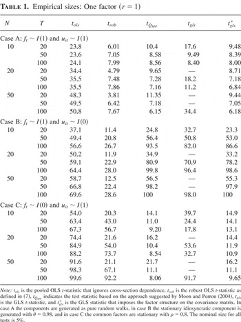
Table 1 reports the actual sizes of the tests. In the top part of the table the results for case A are presented, where both components are generated as random walks (i.e., θ = 1 and ρ = 1). Our theoretical findings summarized in Theorem 1 suggest that in this situation the OLS-based test statistics are biased, whereas the GLS test (t_gls), the modified GLS test (t_gls*), and the

test are asymptotically valid. These results are confirmed by the simulation results presented in Table 1. According to Remark 2, we expect that the actual size of the test converges to 0.6827 as N and T tend to infinity. Indeed, this test statistic is severely biased, with an actual size exceeding 0.5 if N = 50 and T = 100.

Empirical sizes: One factor (r = 1)

Theorem 1(i) indicates that in a single-factor model the robust t-statistic is distributed as the Dickey–Fuller t-statistic. The 5% critical value of this distribution is −1.95 compared to the critical value of −1.645 for the standard normal distribution. Therefore, we expect a moderate positive size bias of the robust OLS t-statistic. Indeed, our Monte Carlo simulations suggest that this test statistic slightly overrejects as T becomes large.

As suggested by our Monte Carlo simulations, the actual sizes of the test statistics that impose the factor structure (

and t_gls*) are close to the nominal size. In contrast, the general GLS t-statistic is severely biased if T is only slightly larger than N. Our results suggest that the nominal size is attained when T is at least 10 times larger than N. This result is in line with our theoretical results that require N²/T → 0 for the distribution to be asymptotically standard normal.

The second part of Table 1 presents the actual sizes of the test if the panel units are cross-cointegrated (case B). We set θ = 0.98 to generate “near-integrated” errors, which seems plausible for many economic applications.

statistic tend to −∞ and therefore the actual size tends to one. This is confirmed by our Monte Carlo simulations, where in large samples the rejection frequencies are close to unity.

The theoretical considerations of Section 6 suggest that in case C the actual sizes of the OLS-based statistics tend to one, whereas the actual sizes of the

and t_gls statistics are expected to converge to the nominal ones as N and T tend to infinity. Setting ρ = 0.8 yields a stationary factor with long-run dynamics that are clearly different from the idiosyncratic components, and the theoretical findings should be relevant in fairly small samples also. The results of our Monte Carlo simulation presented in the third part of Table 1 show that this is indeed the case, as the GLS statistic suffers from size distortions in small samples. It generally has a larger size bias than the

statistic that disappears slowly as T increases.

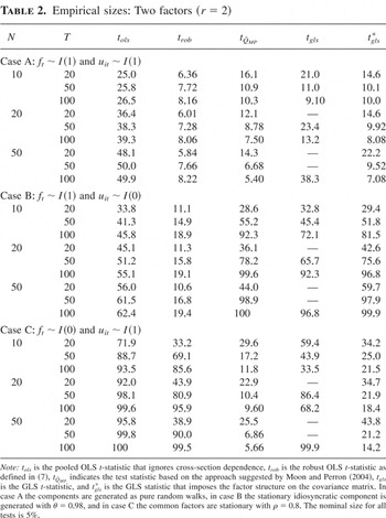
Next we consider a factor model with r = 2, where the factors are generated as f_jt = ρf_j,t−1 + v_jt (j = 1,2) and the idiosyncratic errors are generated as in the single-factor model. The results of the Monte Carlo simulations for the three situations considered in Sections 4–6 are presented in Table 2. In general, the results are similar to the findings based on the single-factor model. A notable difference is that the tests that impose the two-factor structure (

and t_gls*) perform substantially worse in small samples. Furthermore, it is important to note that these tests are computed assuming that the correct number of factors is known. If the number of factors is estimated, e.g., by using the information criteria suggested by Bai and Ng (2002), one can expect that the performance will be even worse.

Empirical sizes: Two factors (r = 2)