2.1 Experimental set-up

A string loop is entrained by rubber wheels mounted on two identical DC motors rotating at the same velocity but in opposite directions (figure 1). The wheels impose the linear velocity $V$ and the angle at which the string is ejected. The transition from a pendent to a self-supporting shape is observed only for strings of low linear mass. We have used a three-ply cotton string, with a very low effective elasticity, of radius $R=5.5\times 10^{-4}~\text{m}$ and density $\unicode[STIX]{x1D70C}_{s}=300~\text{kg}~\text{m}^{-3}$ . Introducing its cross-sectional area $A_{s}=\unicode[STIX]{x03C0}R^{2}$ , the linear mass density is $\unicode[STIX]{x1D70C}_{s}A_{s}=2.88\times 10^{-4}~\text{kg}~\text{m}^{-1}$ , as directly measured using chemistry scales with a resolution better than one percent. The length $\ell$ of the string, the ejection angle of the string at the shooter and the velocity $V$ are our three control parameters.

2.2 Evidence for the hydrodynamic lift of the string

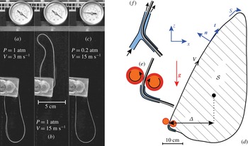
Figure 1 shows low- and high-velocity steady state shapes of the string, which are directly related to the fact that it makes a loop. Indeed, a very long, unclosed string entrained by the same two wheels traces a long inverted catenary trajectory, as expected (Biggins Reference Biggins2014). The role of air becomes clear when performing the experiment at reduced pressure (figure 1 c): despite high kinetic energy that would propel a free string many metres up and away (here $V^{2}/\boldsymbol{g}\simeq 23~\text{m}$ ), the looped string hangs down as for low velocities at atmospheric pressure. Further evidence for the importance of air drag is the possibility of replacing the wheel entrainment (figure 1 e) by an aerodynamic entrainment (figure 1 f).

The string can be safely considered as inextensible: in our experiments the maximum elongation is of order $\unicode[STIX]{x1D70C}_{s}A_{s}V^{2}/EA=10^{-3}$ , based on the string’s measured stiffness $EA=35~\text{N}$ , and tensions of order $\unicode[STIX]{x1D70C}_{s}A_{s}V^{2}=0.03~\text{N}$ for $V=10~\text{m}~\text{s}^{-1}$ . In the steady state, the continuity equation applied to any piece of inextensible string implies that the velocity is tangent everywhere to the string and is constant in modulus. As a consequence, it can be written as $V\boldsymbol{t}$ , where $V$ is imposed by the motor. First consider a simple model in which one would neglect the hydrodynamic drag exerted by the air on the string. Then, the string would be a conservative system whose energy is minimal at equilibrium. The kinetic energy, $\frac{1}{2}\unicode[STIX]{x1D70C}_{s}A_{s}\ell V^{2}$ , does not depend on the shape of the string. As a consequence, such a model predicts that the string shape should always be the one minimising the potential energy, leading to a solution independent of the driving velocity (Walton & Mackenzie Reference Walton and Mackenzie1854, p. 66) – in contrast to the observations reported in figure 1.

Figure 1.

A string loop entrained by two counter-rotating wheels at speed $V$ exhibits a transition from (a) a gravity-dominated regime at low velocity towards (b) a high-velocity regime where the string takes the form of a self-supporting loop. (c) Reducing the pressure from atmospheric pressure to 20 kPa while keeping the high velocity reverts the string back to its lowered configuration. Images (a–c) were processed for readability by subtracting the background and enhancing contrast. Each image is 6.25 cm large. (d) Notations used in the text. The string is entrained by either (e) counter-rotating wheels or (f) by blowing air along a small portion of it.

3.1 A minimal model

The minimal model for the self-sustained string must therefore involve inertia, gravity, string tension and the drag by the surrounding fluid. From dimensional analysis, the drag force per unit length exerted on a string moving along its tangent takes the form $-\unicode[STIX]{x1D6FC}\unicode[STIX]{x1D70C}_{f}R|\boldsymbol{v}|\boldsymbol{v}$ , where $\unicode[STIX]{x1D6FC}$ is a dimensionless ‘skin’ friction, $\unicode[STIX]{x1D70C}_{f}$ the fluid density and $\boldsymbol{v}$ the material velocity. Assuming inextensibility, the equation of motion reads as

(3.1) $$\begin{eqnarray}\unicode[STIX]{x1D70C}_{s}A_{s}\frac{\text{d}\boldsymbol{v}}{\text{d}t}=\unicode[STIX]{x1D70C}_{s}A_{s}\boldsymbol{g}+\frac{\unicode[STIX]{x2202}(T\boldsymbol{t})}{\unicode[STIX]{x2202}s}-\unicode[STIX]{x1D6FC}\unicode[STIX]{x1D70C}_{f}R|\boldsymbol{v}|\boldsymbol{v},\end{eqnarray}$$

where $s$ is the curvilinear coordinate and $\boldsymbol{t}$ the unit tangent vector (figure 1 d). Importantly, the acceleration is the total time derivative of the velocity: $\text{d}/\text{d}t=\unicode[STIX]{x2202}/\unicode[STIX]{x2202}t+\boldsymbol{v}\boldsymbol{\cdot }\boldsymbol{t}(\unicode[STIX]{x2202}/\unicode[STIX]{x2202}s)$ . In the steady state, the continuity equation implies $\boldsymbol{v}=V\boldsymbol{t}$ , resulting in the following force/inertia balance:

(3.2) $$\begin{eqnarray}\unicode[STIX]{x1D70C}_{s}A_{s}\boldsymbol{g}+\frac{\unicode[STIX]{x2202}}{\unicode[STIX]{x2202}s}[(T-\unicode[STIX]{x1D70C}_{s}A_{s}V^{2})\boldsymbol{t}\,\,]-\unicode[STIX]{x1D6FC}\unicode[STIX]{x1D70C}_{f}RV^{2}\boldsymbol{t}=0.\end{eqnarray}$$

The effect of inertia is to shift the tension to negative values by a constant $\unicode[STIX]{x1D70C}_{s}A_{s}V^{2}$ . We will call $T-\unicode[STIX]{x1D70C}_{s}A_{s}V^{2}$ the effective tension, which, contrary to the true tension $T$ , can be negative. We introduce the dimensionless number comparing tension to inertial forces as

(3.3) $$\begin{eqnarray}{\mathcal{T}}=\frac{T}{\unicode[STIX]{x1D70C}_{s}A_{s}V^{2}}.\end{eqnarray}$$

As $\sqrt{T/\unicode[STIX]{x1D70C}_{s}A_{s}}$ is the velocity of transverse waves, the Mach number is simply related to the rescaled tension as ${\mathcal{T}}^{-1/2}$ . The ‘Mach 1’ critical point therefore coincides with ${\mathcal{T}}=1$ and separates a supersonic regime at ${\mathcal{T}}<1$ from a subsonic regime at ${\mathcal{T}}>1$ . The transonic regime ${\mathcal{T}}\sim 1$ is discussed at the end of this article.

3.2 How can the hydrodynamic drag lift the string?

Integrating equation (3.2) over the closed loop, one sees that the weight $\unicode[STIX]{x1D70C}_{s}A_{s}\ell \boldsymbol{g}$ must be balanced by the discontinuity of the effective tension $(T-\unicode[STIX]{x1D70C}_{s}A_{s}V^{2})\boldsymbol{t}$ across the driving point. Indeed, the hydrodynamic drag is constant and tangent to the string, and therefore has a null resultant. The tension is controlled by inextensibility in a way analogous to pressure in incompressible hydrodynamics: its discontinuity is a consequence of hydrodynamic drag, and would be zero in its absence (see § 3.4). The torque of the weight, evaluated at the driving point, is equal to $-\unicode[STIX]{x1D70C}_{s}A_{s}\ell \boldsymbol{g}\unicode[STIX]{x1D6E5}$ , where $\unicode[STIX]{x1D6E5}$ is the horizontal distance between the centre of mass of the string and the driving point. The self-sustained state is therefore characterised by a non-vanishing torque due to weight (figure 1 d). The effective tension on the other hand has a null lever arm at the driving point, and therefore induces no torque. The hydrodynamic torque, obtained by integrating the drag moment along the string, is proportional to the surface area ${\mathcal{S}}$ of the loop, and reads as $2{\mathcal{S}}\unicode[STIX]{x1D6FC}\unicode[STIX]{x1D70C}_{f}RV^{2}$ . Here we have used Green’s theorem to relate the circulation to the area spanned by the loop: $|\oint \boldsymbol{t}\times \boldsymbol{r}\,\text{d}s|=\oint (x\,\text{d}z-z\,\text{d}x)=2\iint _{{\mathcal{S}}}\,\text{d}x\,\text{d}z=2\,{\mathcal{S}}$ . In the steady state, the hydrodynamic torque balances the torque due to the weight. It is therefore the hydrodynamic drag, exerted by the air on the string, which leads to a self-supporting loop. The horizontal displacement of the centre of mass $\unicode[STIX]{x1D6E5}$ increases with $V$ but must remain below $\ell /4$ , by geometrical constraint. One accordingly predicts that the loop becomes slim at high speed, its area decreasing as ${\mathcal{S}}\propto V^{-2}$ .

Figure 2.

(a) The friction coefficient $\unicode[STIX]{x1D6FC}$ decreases slightly as a function of the Reynolds number based on the string radius, ${\mathcal{R}}=\unicode[STIX]{x1D70C}_{f}RV/\unicode[STIX]{x1D702}_{f}$ . Red circles: equation (3.4) with $\unicode[STIX]{x1D6E5}$ and ${\mathcal{S}}$ from the raw shape, blue triangles: equation (3.4) with $\unicode[STIX]{x1D6E5}$ and ${\mathcal{S}}$ of the numerical best fit of the string steady state shape by the theory. The green squares are independent measurements on free falling string segments. The grey diamonds are measurements on two-strand acryl yarn reported by Uno (Reference Uno1972). The dotted curve is the parameter-free prediction in the hydrodynamically smooth regime (3.7) for an infinite straight string. The solid line is the best fit in the hydrodynamically rough regime ( $r_{0}=180~\unicode[STIX]{x03BC}\text{m}$ ). (b) Notations for the drag calculation. The velocity field is assumed to be axisymmetric.

Under the assumption that further dynamical mechanisms may be safely ignored, the torque balance can be used to estimate the hydrodynamic drag from the string shape, namely from the measurement of $\unicode[STIX]{x1D6E5}$ and ${\mathcal{S}}$ :

(3.4) $$\begin{eqnarray}\unicode[STIX]{x1D6FC}=\frac{\unicode[STIX]{x1D70C}_{s}A_{s}\ell \boldsymbol{g}}{2\unicode[STIX]{x1D70C}_{f}RV^{2}}\frac{\unicode[STIX]{x1D6E5}}{{\mathcal{S}}}.\end{eqnarray}$$

3.3 Estimating the turbulent skin drag on the string

The effective drag coefficient deduced experimentally from (3.4) can be compared to theoretical expectations, based on well-established phenomenological laws. Consider an infinite cylinder moving along its axis at constant velocity $V$ (figure 2 b). This is a turbulent boundary layer problem in an axisymmetric geometry. In the steady state the momentum flux across any cylinder of radius $r>R$ must be the same, so that the shear stress $\unicode[STIX]{x1D70E}_{rz}$ decreases as $r^{-1}$ . Using the Prandtl mixing length approach (van Driest Reference van Driest1956; Schlichting & Gersten Reference Schlichting and Gersten2006; Flack & Schultz Reference Flack and Schultz2010), the turbulent Reynolds stress outside the surface (viscous or rough) sublayer then reads as

(3.5) $$\begin{eqnarray}\unicode[STIX]{x1D70E}_{rz}\simeq \unicode[STIX]{x1D70C}_{f}\unicode[STIX]{x1D705}^{2}(r-R)^{2}\left|\frac{\unicode[STIX]{x2202}u_{z}}{\unicode[STIX]{x2202}r}\right|\,\frac{\unicode[STIX]{x2202}u_{z}}{\unicode[STIX]{x2202}r}=-\frac{\unicode[STIX]{x1D6FC}\unicode[STIX]{x1D70C}_{f}V^{2}R}{2\unicode[STIX]{x03C0}r},\end{eqnarray}$$

where $\unicode[STIX]{x1D705}\simeq 0.41$ is the von-Kármán constant. The momentum balance integrates into

(3.6) $$\begin{eqnarray}u_{z}=V-\sqrt{\frac{\unicode[STIX]{x1D6FC}}{2\unicode[STIX]{x03C0}}}\frac{V}{\unicode[STIX]{x1D705}}\log \left[\frac{4R}{r_{0}}\,\frac{\sqrt{r}-\sqrt{R}}{\sqrt{r}+\sqrt{R}}\right],\end{eqnarray}$$

where the integration constant $r_{0}$ is identified as the hydrodynamic roughness in the limit $r_{0}\ll R$ . In the smooth hydrodynamic regime, one expects a roughness $r_{0}\simeq \frac{1}{8}\sqrt{2\unicode[STIX]{x03C0}/\unicode[STIX]{x1D6FC}}\unicode[STIX]{x1D702}_{f}/\unicode[STIX]{x1D70C}_{f}V$ , where the factor $1/8$ is a phenomenological constant determined experimentally in the case of quasi-bidimensional turbulent boundary layers (Schlichting & Gersten Reference Schlichting and Gersten2006, chap 17: logarithmic overlap law). When the viscous sublayer is smaller than the corrugations of the wire, in the hydrodynamically rough regime, one rather expects $r_{0}$ to be a fraction of the geometrical roughness. The velocity must vanish at infinity, which leads to the relation

(3.7) $$\begin{eqnarray}\unicode[STIX]{x1D6FC}=2\unicode[STIX]{x03C0}\frac{\unicode[STIX]{x1D705}^{2}}{\log ^{2}\left[\displaystyle \frac{4R}{r_{0}}\right]}.\end{eqnarray}$$

The velocity tends to $0$ , far from the string, as $1/\sqrt{r}$ . As a consequence, the momentum per unit length stored in the air, $\int 2\unicode[STIX]{x03C0}\unicode[STIX]{x1D70C}_{f}ru_{z}\,\text{d}r$ , is infinite in the steady state (the integral diverges as $r^{3/2}$ ). This means that added mass effects, discussed later, would diverge for an asymptotically long and straight string: they must be limited by the finite size or the finite radius of curvature, which makes their quantitative modelling difficult.

Figure 2 shows that the measured values of $\unicode[STIX]{x1D6FC}$ , using equation (3.4), are almost constant, only slightly decreasing with increasing Reynolds number. The average value $\unicode[STIX]{x1D6FC}\simeq 0.167$ corresponds to a hydrodynamic roughness of $r_{0}\simeq 180~\unicode[STIX]{x03BC}\text{m}\simeq R/3$ – more than ten times larger than the viscous sublayer. This value is consistent with rough surface structures of size comparable to the string radius $R$ , as are formed by the strands making up our three-ply cotton yarn. The skin friction coefficient $\unicode[STIX]{x1D6FC}$ was also independently measured in a free fall experiment using string segments attached to an excess weight. This drag is slightly lower, possibly due to the absence of counter-moving string. Measurements of longitudinal air drag of very long cylinders are scarce in the literature. The air drag of textile fibres is exploited in air-jet looms, but studies mostly consider short segments in non-homogeneous airflow. As a notable exception, Selwood (Reference Selwood1962), using an elegant set-up to drag 20 m of nylon fibre through still air, reports a drag coefficient of 0.093 at the highest Reynolds number ${\mathcal{R}}=60$ – well below our values as expected for a much smoother filament. Measurements on long ( $\ell /R>4000$ ) rough two-filament yarn by Uno (Reference Uno1972) on the other hand are in accordance with our data (figure 2 a) and confirm that plied yarn has a larger effective roughness than mono-filaments.

Figure 3.

A typical experimental curve observed just above the threshold is shown in blue on both panels, obtained for $V_{0}=5.29~\text{m}~\text{s}^{-1}$ . (a) Solutions to equation (3.8) for various initial conditions and ${\mathcal{A}}=1.44$ . Red are possible upper branches of the steady string loop, green possible lower branches. Note the up $\rightarrow$ down, red $\rightarrow$ green symmetry. In a given experiment (blue) the upper and lower parts of the loop each match one of the solutions. Note that the propelling system is on the left. Lengths are in units of $V^{2}/\boldsymbol{g}$ . (b) Change of the selected shape as the drag parameter ${\mathcal{A}}$ increases (from top to bottom: 1.00798, 1.02168, 1.05893, 1.1602, 1.43546, 2.18369, 4.21761, 9.74637), keeping the ejection angle and string length constant. The shapes have been superimposed at the singularity, whereas experimentally the leftmost point (corresponding to the shooter) is fixed. Lengths are in units of $V_{0}^{2}/\boldsymbol{g}$ .

3.4 Predicted shape

We express the curvilinear coordinate $s=SV^{2}/\boldsymbol{g}$ along the string in terms of its dimensionless counterpart $S$ using $V^{2}/\boldsymbol{g}$ as the characteristic length. The equation (3.2), projected onto the tangent and the normal vectors, yields

(3.8a ) $$\begin{eqnarray}\displaystyle \frac{\text{d}{\mathcal{T}}}{\text{d}S} & = & \displaystyle \sin \unicode[STIX]{x1D703}+{\mathcal{A}},\end{eqnarray}$$

(3.8b ) $$\begin{eqnarray}\displaystyle \frac{\text{d}\unicode[STIX]{x1D703}}{\text{d}S} & = & \displaystyle \frac{\cos \unicode[STIX]{x1D703}}{{\mathcal{T}}-1},\end{eqnarray}$$

$V^{2}$

(3.9) $$\begin{eqnarray}{\mathcal{A}}=\unicode[STIX]{x1D6FC}\frac{\unicode[STIX]{x1D70C}_{f}RV^{2}}{\unicode[STIX]{x1D70C}_{s}A_{s}\boldsymbol{g}}.\end{eqnarray}$$

Equation (3.8a ) integrates to ${\mathcal{T}}\simeq {\mathcal{T}}_{0}+{\mathcal{A}}S+Z$ , where $Z$ is the altitude rescaled by $V^{2}/\boldsymbol{g}$ and ${\mathcal{T}}_{0}$ the tension immediately after the driving point.

Equation (3.8b ) is singular at the critical point ${\mathcal{T}}=1$ , except if the latter is located at the point whose tangent is vertical ( $\unicode[STIX]{x1D703}=3\unicode[STIX]{x03C0}/2$ ). In this case, equation (3.8) admits, around the critical point, an asymptotic solution of the form

(3.10) $$\begin{eqnarray}\displaystyle {\mathcal{T}} & {\sim} & \displaystyle 1+({\mathcal{A}}-1)S,\end{eqnarray}$$

(3.11) $$\begin{eqnarray}\displaystyle \unicode[STIX]{x1D703}(s) & {\sim} & \displaystyle 3\unicode[STIX]{x03C0}/2-CS^{1/({\mathcal{A}}-1)}.\end{eqnarray}$$

This solution is used as a starting point, parameterised by ${\mathcal{A}}$ and $C$ , for numerical integration of equation (3.8). Figure 3(a) shows the family of solutions for a fixed value of the drag ${\mathcal{A}}$ . Loop shapes near critical drag (blue example in figure 3) are reproduced well, letting ${\mathcal{A}}$ be an adjustable parameter. Figure 3(b) shows solutions that differ in velocity $V$ , but share the same ejection angle and string length. The succession of shapes shows the transition from gravity-dominated shapes to lifted states.

Figure 4.

(a) Position of transverse wavefronts on a string above the threshold ( $V_{0}=5.29~\text{m}~\text{s}^{-1}$ , same experiment as in figure 3). Seven deformations were tracked on both upper (red) and lower (green) branches, and their trajectories superimposed by taking $t=0$ upon leaving the propelling wheels. Wavefronts travelling in the direction of the string movement on the upper branch and in the reverse direction on the lower branch slow down critically as they approach the singularity at $s=0$ . The black lines are calculated from the tension shown in (b). (b) The string tension, corresponding to the best shape fit of upper and lower parts by our model (inset), increases along the string in the direction of string motion. ${\mathcal{T}}=1$ defines the singular point, which defines the origin of the curvilinear coordinate $s$ in both graphs.

3.5 Wave propagation

The theory predicts that all upper branches move at supersonic speeds with respect to transverse waves ( ${\mathcal{T}}<1$ ), while in contrast lower branches are subsonic ( ${\mathcal{T}}>1$ ). This produces a white hole analogue similar to what can be achieved using surface waves on a flowing fluid (Schützhold & Unruh Reference Schützhold and Unruh2002; Rousseaux et al. Reference Rousseaux, Maïssa, Mathis, Coullet, Philbin and Leonhardt2010). As opposed to finite time singularities that occur in the motion of open-ended strings (McMillen & Goriely Reference McMillen and Goriely2003; Brun et al. Reference Brun, Audoly, Goriely and Vella2016), the transsonic singularity in the propelled loop is stationary. To test its existence experimentally, we take advantage of the fact that the knot which ties the string into a loop produces small deformations of the loop shape at each passage through the propelling wheels. We tracked the position of seven deformations on both upper and lower branches in one given experiment, and find that these transverse perturbations exhibit a critical slowing down as they travel along the string (figure 4 a). This is a signature of the singularity: transverse waves propagate at a speed $\pm \sqrt{T/\unicode[STIX]{x1D70C}_{s}A_{s}}$ relative to the moving string. Waves that propagate upstream (that is, in the direction opposite to the string movement) therefore appear to move at a speed $V-\sqrt{T/\unicode[STIX]{x1D70C}_{s}A_{s}}$ in the laboratory reference frame. This speed is positive (moving with the string) on the upper branch (where $\sqrt{T/\unicode[STIX]{x1D70C}_{s}A_{s}}=\sqrt{{\mathcal{T}}}V<V$ ) and negative on the lower branch ( $\sqrt{T/\unicode[STIX]{x1D70C}_{s}A_{s}}>V$ ), so that the perturbations travel towards the singularity on either side of it. The best shape fit of this experiment by equations (3.8) yields a tension curve ${\mathcal{T}}(s)$ (figure 4 b) from which we deduce trajectories $\text{d}s/\text{d}t=V(1-\sqrt{{\mathcal{T}}})$ that closely match the observations (figure 4 a): this confirms the existence of the singularity and validates the minimal model, immediately above the threshold.

4.1 Departure from the pear shape

When the speed is increased above the threshold, the shape becomes widest in the middle and tapers at both ends, in the manner of a spindle. The spindle becomes slimmer with increasing velocity (figure 5 a), in accordance with the minimal model, and in particular the torque balance of (3.4). At high speed, however, the string exhibits an angular point at the singularity, which does not correspond to any of the smooth pear-shaped solutions of figure 3. An example is shown in figure 5(b,c). The upper and lower branches are still fitted well by (3.8), on condition that both the angle and the tension are allowed to be discontinuous across the singularity. The discontinuity vanishes near the onset of the self-supporting loop regime (figure 5 a), where the string has a vertical tangent at the singular point and the shape is described well by a pear-shaped solution.

Figure 5.

(a) Aspect ratio (blue squares) and angle discontinuity at the singular point (yellow circles) of the string loop at different velocities. Note the factor $2$ in $L/2W$ added to get a common scale. (b) Experimental loop shape (black, $\ell =3.4~\text{m}$ , $V=9.53~\text{m}~\text{s}^{-1}$ ) with superposed best fits by the simplified model (3.8) of the upper (red) and lower (green) parts. (c) Detailed view of the vicinity of the singularity at the top right, showing that the apparent angle discontinuity is regularised in the experiment.

4.2 Dynamical mechanisms in the vicinity of the critical point

As the upper and lower branches are still described well by the minimal model outside the class of smooth ‘pear’ solutions, some further dynamical mechanism must show up and dominate only in the vicinity of the singularity, and produce the small slightly asymmetric bend of finite curvature that can be observed in figure 5(c). Placing an obstacle (a solid plate) near the tip causes important changes in this curved upper region around the critical point. This directly shows that non-local effects are present. Momentum is transferred across the loop via the entrained fluid, especially between counter-moving upper and lower branches near the end where the shape tapers. As boundary layers develop along a straight string, the drag force diminishes (Gould & Smith Reference Gould and Smith1980). In contrast we expect the drag coefficient $\unicode[STIX]{x1D6FC}$ to increase when the string is curved, explaining the extra dissipation associated with the sudden change of tension around the corner.

4.3 Added mass effect and hydrodynamic torque

As air flows along the moving curved string, there must be an added mass effect (that is, a hydrodynamic force component normal to the string) that can be estimated using a simple momentum balance argument. Let $\unicode[STIX]{x1D6FF}$ denote the effective thickness of the air layer that flows at the speed $V$ of the string and that changes direction when the string is curved. The momentum flux of this layer is then $\unicode[STIX]{x1D70C}_{f}\int _{R+r_{0}}^{R+\unicode[STIX]{x1D6FF}}2\unicode[STIX]{x03C0}ru_{z}^{2}\,\text{d}r\simeq 8\unicode[STIX]{x03C0}\unicode[STIX]{x1D70C}_{f}R\unicode[STIX]{x1D6FF}/\log ^{2}(4R/r_{0})$ , and the centripetal force required for a direction change is proportional to this flux times curvature. The reaction on the string can therefore be included by replacing $\unicode[STIX]{x1D70C}_{s}A_{s}$ with $\unicode[STIX]{x1D70C}_{s}A_{s}+\unicode[STIX]{x1D70C}_{f}A_{f}$ , with $A_{f}=8\unicode[STIX]{x03C0}\unicode[STIX]{x1D6FF}R/\log ^{2}(4R/r_{0})$ , in the inertial term of the momentum balance. We will not try here to model $\unicode[STIX]{x1D6FF}$ , which may depend on the whole shape of the string. As an upper bound, one may consider the thickness of a boundary layer developing over a length ${\sim}\ell$ , obeying $\unicode[STIX]{x1D6FF}\log (\unicode[STIX]{x1D6FF}/r_{0})\sim \ell$ . As $\unicode[STIX]{x1D6FF}$ is at most ${\sim}10~\text{cm}$ , the added mass effect can only increase the apparent density by $10\,\%$ of $\unicode[STIX]{x1D70C}_{s}A_{s}$ .

Additional effects come into play when we consider a string of finite diameter, for which we may notably have local torque $N$

(4.1) $$\begin{eqnarray}\displaystyle (\unicode[STIX]{x1D70C}_{s}A_{s}+\unicode[STIX]{x1D70C}_{f}A_{f})V^{2}\frac{\unicode[STIX]{x2202}}{\unicode[STIX]{x2202}s}\boldsymbol{t} & = & \displaystyle \unicode[STIX]{x1D70C}_{s}A_{s}\boldsymbol{g}+\frac{\unicode[STIX]{x2202}}{\unicode[STIX]{x2202}s}(T\boldsymbol{t}+N\boldsymbol{n})-\unicode[STIX]{x1D6FC}\unicode[STIX]{x1D70C}_{f}RV^{2}\boldsymbol{t},\end{eqnarray}$$

(4.2) $$\begin{eqnarray}\displaystyle (\unicode[STIX]{x1D70C}_{s}I_{s}+\unicode[STIX]{x1D70C}_{f}I_{f})V^{2}\frac{\unicode[STIX]{x2202}^{2}\unicode[STIX]{x1D703}}{\unicode[STIX]{x2202}s^{2}} & = & \displaystyle N,\end{eqnarray}$$

where $I_{s}=\unicode[STIX]{x03C0}R^{4}/4$ is the string’s moment of inertia and $I_{f}=4\unicode[STIX]{x03C0}\unicode[STIX]{x1D6FF}^{3}R/3\log ^{2}(4R/r_{0})$ the added mass effect, which is a first-order description of the hydrodynamic moment exerted on the string. This time, the added mass effect is typically $10^{3}$ larger than the solid contribution (prefactor $10^{-7}$ versus $10^{-10}$ in the dimensionless equations), and also larger than the moment resulting from the string’s elastic bending stiffness (De Langre et al. Reference De Langre, Païdoussis, Doaré and Modarres-Sadeghi2007). The latter is estimated from the elasto-gravitary length $a\simeq 3~\text{cm}$ – measured from the deflection of cantilevers made of string – to approximately $-EI\,\boldsymbol{g}^{2}/\unicode[STIX]{x1D70C}_{s}AV^{6}\simeq -\boldsymbol{g}^{3}a^{3}/V^{6}\simeq -3\times 10^{-8}$ . Note that the signs of inertial and elastic stiffness are opposite, so the relative importance of inertial and elastic stiffness has a strong impact on the behaviour of the solution near the singularity. The torque contribution becomes of order 1 when the curvature and its derivatives change significantly over length scales smaller than $5\times 10^{-3}\,V^{2}/\boldsymbol{g}\simeq 5~\text{cm}$ , compatible with the scale at which the string bends near the singularity (figure 5 c).

These examples of higher-order hydrodynamic effects are by no means exhaustive: the dynamics of finite-size bodies accelerating in flows is notoriously hard to model and includes history forces and drag corrections (Mordant & Pinton Reference Mordant and Pinton2000; Calzavarini et al. Reference Calzavarini, Volk, Lévêque, Pinton and Toschi2012). Understanding the string dynamics in the vicinity of the singularity will thus require a much more involved analysis of the hydrodynamics of the surrounding fluid.

4.4 Perspectives

The drag on cylinders in axial flow is dominated by the pressure contributions at the end caps for all but very elongated cylinders. Loops on the other hand experience only skin drag, making the experiment discussed here an ideal set-up for its study, including effects of finite size. A promising application in the textile industry may be the estimation of axial drag coefficients of fibres simply from the transition speed between gravitational and lifted states, and from the string’s linear mass. Such a low-tech method may be of direct interest to textile producers wishing to adjust an air-jet loom to a new fibre type, without the need for a sophisticated and costly wind channel and drag measurement apparatus.

On a more fundamental level, the formal resemblance of string dynamics with one-dimensional hydrodynamics, with tension playing the role of pressure, suggest a rich field of study both in steady and unsteady cases. The mathematical structure of the theoretical problem is particularly interesting, as the dynamical equations are easy to express in Lagrangian coordinates but the boundary conditions (obstacles for instance) are typically Eulerian. The creation of lift through axial drag forces, mediated by tension, is just a hint at more complex behaviour to be expected in unsteady situations. Of particular interest may be the interactions between moving filaments in turbulent flows, and propulsion systems involving several filaments (tentacles).