1. Introduction
Two-layer density stratified fluid systems are observed in many natural and engineering situations. The one observed at estuaries which are generated by the lighter fresh water from rivers flowing onto the heavier brine may be one of the most familiar examples. The existence of the interface brings about a new wave mode called the ‘interfacial waves’, for which the amplitude of the displacement of the interface is larger than that of the free surface. These interfacial waves and their interactions with the surface waves are considered to be relevant for many phenomena such as resuspension of mud in lakes and estuaries, seiches observed in many mid-latitude lakes, etc. (Turner Reference Turner1973; Osborne & Burch Reference Osborne and Burch1980).
In various wave phenomena, resonant interactions between waves play crucial roles (Phillips Reference Phillips1960). For a two-layer fluid system with an interface and a free surface, it has long been known (Ball Reference Ball1964) that there are two types of three-wave resonant interactions. The first one, called class 1, occurs between two oppositely propagating surface waves and an interfacial wave, while the second one, called class 2, occurs among two oppositely propagating interfacial waves and a surface wave. Resonant interactions which include multiple surface waves propagating in the same direction has not been known until quite recently. Alam (Reference Alam2012) showed that a new type of three-wave resonance, called class 3, is possible between two surface waves and an interfacial wave in which all the three waves propagate in the same direction. In wind-generated waves on the water surface, it is natural that the waves propagate predominantly in the direction of the wind, hence this class 3 resonance is expected to play much more important roles than the resonances of the other classes in the process of nonlinear energy transfer from wind-generated surface waves to interfacial waves.
The dispersion relation
 ${\it\omega}=\sqrt{gk\tanh kh}$
for the surface gravity waves in a single-layer fluid is of non-decay type, and the three-wave resonance condition
 $$\begin{eqnarray}k_{1}\pm k_{2}\pm k_{3}=0\quad \text{and}\quad {\it\omega}_{1}\pm {\it\omega}_{2}\pm {\it\omega}_{3}=0,\end{eqnarray}$$
cannot be met for any combination of the wavenumbers
 $(k_{1},k_{2},k_{3})$
(Phillips Reference Phillips1960). Resonant interactions between waves are possible only among four or more waves, and this fact makes the evolution of the energy spectrum of surface gravity waves very slow with the time scale of
 $O(1/{\it\omega}_{0}{\it\epsilon}^{4})$
, with
 ${\it\omega}_{0}$
and
 ${\it\epsilon}$
being the typical frequency and non-dimensional amplitude, respectively (Hasselmann Reference Hasselmann1962; Zakharov, L’vov & Falkovich Reference Zakharov, L’vov and Falkovich1992). When the effect of surface tension is taken into account, the dispersion relation is given by
 ${\it\omega}=\sqrt{(gk+{\it\tau}k^{3}/{\it\rho})\tanh kh}$
, which is of decay type and the three-wave resonance becomes possible (McGoldrick Reference McGoldrick1965). The newly found class 3 resonance in a two-layer fluid suggests the possibility that the surface wave spectrum can change much faster in the time scale of
 $O(1/{\it\omega}_{0}{\it\epsilon}^{2})$
, without resorting to the effect of surface tension but by being mediated by interfacial waves.
The aim of this study is to investigate the evolution of the energy spectra of the surface and the interfacial waves due to the three-wave resonant interactions among them by direct numerical simulations of the governing equations for the two-layer fluid system. In § 2 we describe the two-layer fluid system and the governing equations for it. The method and various settings of the numerical simulations are explained in §§ 3 and 4, and the results obtained are shown in § 5. Conclusions and discussion are given in § 6.
2. Two-layer fluid system
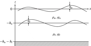
We investigate wave motions in a two-layer fluid system as shown in figure 1. In each of the layers we assume that the fluid is homogeneous, incompressible, immiscible and inviscid, and that the motion is irrotational and the fluid velocity is expressed as the gradient of the velocity potential. The bottom is flat, and the motion is assumed to be two-dimensional in the vertical plane. The effect of surface tension is neglected.
Definition sketch of a two-layer fluid system.

We employ a Cartesian coordinate system with the horizontal
 $x$
axis on the mean free surface and the vertical
 $z$
axis pointing upward. Then the equations governing the motion of the two-layer fluid system are given as follows:
 $$\begin{eqnarray}\displaystyle & \displaystyle {\rm\nabla}^{2}{\it\phi}_{u}=0,\quad -h_{u}+{\it\eta}_{l}<z<{\it\eta}_{u}, & \displaystyle\end{eqnarray}$$
 $$\begin{eqnarray}\displaystyle & \displaystyle {\rm\nabla}^{2}{\it\phi}_{l}=0,\quad -h_{u}-h_{l}<z<-h_{u}+{\it\eta}_{l}, & \displaystyle\end{eqnarray}$$
 $$\begin{eqnarray}\displaystyle & \displaystyle {\it\eta}_{u,t}+{\it\eta}_{u,x}{\it\phi}_{u,x}-{\it\phi}_{u,z}=0,\quad z={\it\eta}_{u}, & \displaystyle\end{eqnarray}$$
 $$\begin{eqnarray}\displaystyle & \displaystyle {\it\phi}_{u,t}+{\textstyle \frac{1}{2}}({\it\phi}_{u,x}^{2}+{\it\phi}_{u,z}^{2})+g{\it\eta}_{u}=0,\quad z={\it\eta}_{u}, & \displaystyle\end{eqnarray}$$
 $$\begin{eqnarray}\displaystyle & \displaystyle {\it\eta}_{l,t}+{\it\eta}_{l,x}{\it\phi}_{u,x}-{\it\phi}_{u,z}=0,\quad z=-h_{u}+{\it\eta}_{l}, & \displaystyle\end{eqnarray}$$
 $$\begin{eqnarray}\displaystyle & \displaystyle {\it\eta}_{l,t}+{\it\eta}_{l,x}{\it\phi}_{l,x}-{\it\phi}_{l,z}=0,\quad z=-h_{u}+{\it\eta}_{l}, & \displaystyle\end{eqnarray}$$
 $$\begin{eqnarray}\displaystyle & & \displaystyle {\it\rho}_{u}[{\it\phi}_{u,t}+{\textstyle \frac{1}{2}}({\it\phi}_{u,x}^{2}+{\it\phi}_{u,z}^{2})+g{\it\eta}_{l}]\nonumber\\ \displaystyle & & \displaystyle \quad -\,{\it\rho}_{l}[{\it\phi}_{l,t}+{\textstyle \frac{1}{2}}({\it\phi}_{l,x}^{2}+{\it\phi}_{l,z}^{2})+g{\it\eta}_{l}]=0,\quad z=-h_{u}+{\it\eta}_{l},\end{eqnarray}$$
 $$\begin{eqnarray}\displaystyle & & \displaystyle {\it\phi}_{l,z}=0,\quad z=-h_{u}-h_{l},\end{eqnarray}$$
where the densities and the depths of the upper and the lower layers are denoted, respectively, by
 ${\it\rho}_{u}$
,
 $h_{u}$
, and
 ${\it\rho}_{l}$
,
 $h_{l}$
, the free surface and the interface displacements are denoted, respectively, by
 ${\it\eta}_{u}(x,t)$
,
 ${\it\eta}_{l}(x,t)$
, and the velocity potentials of the upper and the lower layers are denoted, respectively, by
 ${\it\phi}_{u}(x,z,t)$
and
 ${\it\phi}_{l}(x,z,t)$
.
The system of equations (2.1) admits a linear solution corresponding to a monochromatic wavetrain
 $\propto \text{e}^{\text{i}(kx-{\it\omega}t)}$
with infinitesimal amplitude. The frequency
 ${\it\omega}$
is related to the wavenumber
 $k$
by the linear dispersion relation
 $$\begin{eqnarray}(1+RT_{u}T_{l}){\it\omega}^{4}-gk(T_{u}+T_{l}){\it\omega}^{2}+(1-R)g^{2}k^{2}T_{u}T_{l}=0,\end{eqnarray}$$
where
 $T_{u}=\tanh kh_{u}$
,
 $T_{l}=\tanh kh_{l}$
and the density ratio
 $R={\it\rho}_{u}/{\it\rho}_{l}$
. The dispersion relation (2.2) is biquadratic with respect to
 ${\it\omega}$
, and has four solutions
 $\pm {\it\omega}_{s}$
,
 $\pm {\it\omega}_{i}$
for each
 $k$
with
 ${\it\omega}_{s}>{\it\omega}_{i}$
. In the mode corresponding to the larger (smaller) value of
 ${\it\omega}$
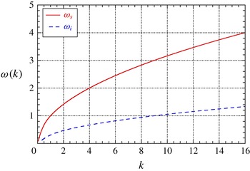
, the amplitude of the surface displacement is larger (smaller) than that of the interface displacement, and we call it the ‘surface (interfacial) wave’. As an example of the dispersion relation, we show in figure 2
 ${\it\omega}_{s}$
and
 ${\it\omega}_{i}$
as functions of
 $k$
when
 $h_{u}=1$
,
 $h_{l}=2$
and
 $R=0.80$
.
The linear dispersion relation (
 $h_{u}=1$
,
 $h_{l}=2$
,
 $R=0.80$
).

3. Methods
3.1. Numerical method
The system of equations (2.1) can be rewritten as the evolution equations for
 ${\it\eta}_{u}$
,
 ${\it\phi}_{u}^{S}$
,
 ${\it\eta}_{l}$
,
 ${\it\psi}^{I}$
as follows (Alam, Liu & Yue Reference Alam, Liu and Yue2009):
 $$\begin{eqnarray}\displaystyle & \displaystyle {\it\eta}_{u,t}=-{\it\eta}_{u,x}{\it\phi}_{u,x}^{S}+(1+{\it\eta}_{u,x}^{2}){\it\phi}_{u,z},\quad z={\it\eta}_{u}, & \displaystyle\end{eqnarray}$$
 $$\begin{eqnarray}\displaystyle & \displaystyle {\it\phi}_{u,t}^{S}=-g{\it\eta}_{u}-{\textstyle \frac{1}{2}}({\it\phi}_{u,x}^{S})^{2}+{\textstyle \frac{1}{2}}(1+{\it\eta}_{u,x}^{2}){\it\phi}_{u,z}^{2},\quad z={\it\eta}_{u}, & \displaystyle\end{eqnarray}$$
 $$\begin{eqnarray}\displaystyle & \displaystyle {\it\eta}_{l,t}=-{\it\eta}_{l,x}{\it\phi}_{u,x}^{I}+(1+{\it\eta}_{l,x}^{2}){\it\phi}_{u,z},\quad z=-h_{u}+{\it\eta}_{l}, & \displaystyle\end{eqnarray}$$
 $$\begin{eqnarray}\displaystyle & & \displaystyle {\it\psi}_{,t}^{I}={\textstyle \frac{1}{2}}[R({\it\phi}_{u,x}^{I})^{2}-({\it\phi}_{l,x}^{I})^{2}]+{\textstyle \frac{1}{2}}(1+{\it\eta}_{l,x}^{2})({\it\phi}_{l,z}^{2}-R{\it\phi}_{u,z}^{2})-g{\it\eta}_{l}(1-R),\quad z=-h_{u}+{\it\eta}_{l},\nonumber\\ \displaystyle & & \displaystyle\end{eqnarray}$$
where
 ${\it\phi}_{u}^{S}(x,t)$
and
 ${\it\psi}^{I}(x,t)$
are defined by
 $$\begin{eqnarray}{\it\phi}_{u}^{S}(x,t)={\it\phi}_{u}(x,{\it\eta}_{u},t),\quad {\it\psi}^{I}(x,t)={\it\phi}_{u}(x,-h_{u}+{\it\eta}_{l},t)-R{\it\phi}_{u}(x,-h_{u}+{\it\eta}_{l},t).\end{eqnarray}$$
The system can be formulated as a Hamiltonian system, for which the total energy (i.e. the sum of the kinetic and the potential energies) is the Hamiltonian,
 ${\it\eta}_{u}$
,
 ${\it\eta}_{l}$
are the canonical coordinates, and
 ${\it\phi}_{u}^{S}$
,
 ${\it\psi}^{I}$
are the canonical momentums (Ambrosi Reference Ambrosi2000).
In order to evaluate the time derivatives of
 ${\it\eta}_{u}$
,
 ${\it\phi}_{u}^{S}$
,
 ${\it\eta}_{l}$
,
 ${\it\psi}^{I}$
by (3.1), we need to solve the boundary value problems of Laplace equations for
 ${\it\phi}_{u}$
,
 ${\it\phi}_{l}$
as specified by (2.1). For this purpose we employ the high-order spectral (HOS) method developed by Alam et al. (Reference Alam, Liu and Yue2009). The HOS method is originally developed by Dommermuth & Yue (Reference Dommermuth and Yue1987) and West et al. (Reference West, Brueckner, Janda, Milder and Milton1987) for surface waves in a single-layer fluid, and Alam et al. have extended it to the two-layer fluid system. In the HOS method the potentials
 ${\it\phi}_{u}$
and
 ${\it\phi}_{l}$
are expanded in perturbation series with respect to the amplitude as
 ${\it\phi}_{u}(x,z,t)=\sum _{m=1}^{M}{\it\phi}_{u}^{(m)}(x,z,t)$
and
 ${\it\phi}_{l}(x,z,t)=\sum _{m=1}^{M}{\it\phi}_{l}^{(m)}(x,z,t)$
, and the boundary conditions at the free surface and the interface are also Taylor expanded around the undisturbed positions. Thus, the original single boundary value problem for
 ${\it\phi}_{u}(x,z,t)$
in a region with a complicated boundary shape delineated by
 $z={\it\eta}_{u}(x,t)$
and
 $z=-h_{u}+{\it\eta}_{l}(x,t)$
is transformed into a series of boundary value problems for
 ${\it\phi}_{u}^{(m)}(x,z,t)~(m=1,\dots ,M)$
in a region with a much simpler boundary shape delineated by
 $z=0$
and
 $z=-h_{u}$
which can easily be solved sequentially starting from the lowest-order problem. The problem for
 ${\it\phi}_{l}(x,z,t)$
is also solved in the same way. Since we are mainly interested in the process of three-wave resonance in this study, the truncation order
 $M$
is chosen to be
 $M=2$
.
The integration of (3.1) with respect to
 $t$
is performed by the fourth-order Runge–Kutta method with a suitably chosen fixed timestep. In all of the numerical simulations, the mass, the time and the length are normalized so that
 ${\it\rho}_{l}=1$
,
 $h_{u}=1$
and
 $g=1$
.
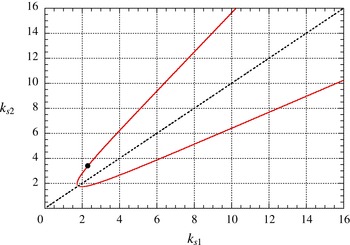
The wavenumbers of the two surface waves satisfying the class 3 resonance condition (3.3) (
 $h_{l}=2$
,
 $R=0.8$
).

3.2. Reproduction of the class 3 resonance
Before proceeding to the investigation on an irregular wave field with a continuous spectrum, we first reproduce the class 3 resonance among a single triad of waves as a test of the numerical code. Figure 3 shows the wavenumbers
 $k_{s1}$
and
 $k_{s2}$
of the two surface waves which satisfy the conditions of class 3 triad resonance
 $$\begin{eqnarray}k_{s2}=k_{s1}\pm k_{i},\quad {\it\omega}_{s2}={\it\omega}_{s1}\pm {\it\omega}_{i},\end{eqnarray}$$
when
 $h_{l}=2$
and
 $R=0.8$
. We choose the point
 $k_{s1}=2.3$
,
 $k_{s2}=3.4$
(marked by ● in the figure) on the ‘resonance curve’, construct the initial wave field as a superposition of these two surface waves only, and see whether the interfacial wave with
 $k_{i}=1.1$
, which is supposed to be in class 3 resonance with these two surface waves, is generated automatically.
It is well known (see, e.g., Craik Reference Craik1985) that the amplitudes
 $a_{s1}$
,
 $a_{s2}$
,
 $a_{i}$
of the three waves which satisfy the resonance condition
 $k_{s2}=k_{s1}+k_{i}$
,
 ${\it\omega}_{s2}={\it\omega}_{s1}+{\it\omega}_{i}$
evolve according to
 $$\begin{eqnarray}\frac{\text{d}a_{s1}}{\text{d}t}=\text{i}{\it\gamma}_{1}a_{s2}a_{i}^{\ast },\quad \frac{\text{d}a_{s2}}{\text{d}t}=\text{i}{\it\gamma}_{2}a_{s1}a_{i},\quad \frac{\text{d}a_{i}}{\text{d}t}=\text{i}{\it\gamma}_{3}a_{s1}^{\ast }a_{s2},\end{eqnarray}$$
where the asterisk denotes complex conjugate and the interaction coefficients
 ${\it\gamma}_{1}$
,
 ${\it\gamma}_{2}$
,
 ${\it\gamma}_{3}$
are some complicated real-valued functions of (
 $h_{l}$
,
 $R$
) and (
 $k_{s1}$
,
 $k_{s2}$
,
 $k_{i}$
). The analytical expressions for
 ${\it\gamma}$
can be obtained by a standard procedure, such as applying a multiple time-scale expansion to (2.1), then requiring the non-secular conditions, and so on. When
 $(h_{l},R)=(2,0.8)$
and
 $(k_{s1},k_{s2},k_{i})=(2.3,3.4,1.1)$
,
 ${\it\gamma}_{1}=-10.4$
,
 ${\it\gamma}_{2}=-8.5$
and
 ${\it\gamma}_{3}=-4.7\times 10^{-2}$
. Of course, the values of
 ${\it\gamma}$
depend on the definition of the amplitude
 $a$
of each wavetrain, and the values cited above are those when
 $a$
denotes the amplitude of the surface displacement
 ${\it\eta}_{u}$
associated to each of the waves.
Since
 $a_{i}=0$
at
 $t=0$
in this numerical experiment, equation (3.4) implies that
 $a_{s1},a_{s2}\approx \text{const.}$
, and
 $|a_{I}|\sim {\it\gamma}_{3}|a_{s1}a_{s2}|t$
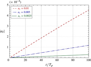
in the initial stage of the evolution. Figure 4 shows
 $|a_{I}|$
as a function of
 $t$
for three cases with
 $a_{s1}=a_{s2}=0.0025$
, 0.005 and 0.01. It can be clearly observed that
 $|a_{I}|$
grows linearly in
 $t$
and its growth rate is in proportion to
 $|a_{s1}a_{s2}|$
as expected. It can also be confirmed that the growth rate of
 $|a_{I}|$
obtained numerically agrees quite well with the value analytically estimated from
 ${\it\gamma}_{3}$
of (3.4). By performing much longer numerical simulations, we have also reproduced the periodic energy exchange among the three waves in resonance, which corresponds to the exact solution of (3.4) expressed in terms of Jacobian elliptic functions.
The linear growth of the interfacial wave by the class 3 triad resonance (
 $h_{l}=2$
,
 $R=0.8$
).

4. Settings of numerical simulations
The energy spectra
 $S_{s}(k)$
,
 $S_{i}(k)$
of the surface waves and the interfacial waves, respectively, at
 $t=0$
are given by
 $$\begin{eqnarray}\displaystyle S_{s}(k)=A\left(\frac{k}{k_{p}}\right)^{-3}\exp \left[-\frac{5}{4}\left(\frac{k}{k_{p}}\right)^{-2}\right]\quad (k>0),\quad S_{s}(k)=0\quad (k\leqslant 0),\end{eqnarray}$$
 $$\begin{eqnarray}\displaystyle S_{i}(k)=0\quad (-\infty <k<\infty ).\end{eqnarray}$$
Thus, the initial wave field consists only of the surface waves propagating in the positive
 $x$
direction, and there is no energy in the interfacial waves. The functional form of
 $S_{s}(k)$
comes from the well-known Pierson–Moskowitz spectrum for ocean waves, but it does not have any special meaning for the two-layer fluid system studied here. The parameters
 $A$
and
 $k_{p}$
control the energy density of the wave field and the wavenumber at the peak of
 $S_{s}(k)$
at
 $t=0$
, respectively. The initial conditions for
 ${\it\eta}_{u},{\it\phi}_{u}^{S},{\it\eta}_{l},{\it\psi}^{I}$
are calculated so that they are consistent with the spectra (4.1). The phase constant of each component wave is given by a uniform random number.
The time evolution is traced numerically up to
 $t=1000T_{p}$
, where
 $T_{p}$
being the period corresponding to the surface wave with wavenumber
 $k_{p}$
. The wavenumber space is truncated at
 $|k|=10k_{p}$
. The number of mesh points in the physical space used in the HOS method is
 $n=2^{18}$
, then the number of independent wavenumbers free from aliasing error is 174 760
 $(=(n/3-1)\times 2)$
. For each set of parameter settings, we repeat the numerical experiment three times by changing the initial phase of each component wave, then take the average over the three results. In all of the following discussion concerning the spectra, the wavenumber resolution
 ${\rm\Delta}k$
is
 $0.1$
. In a single bin with width
 ${\rm\Delta}k$
, there exist some 750 independent component waves used in the numerical simulation when
 $k_{p}=3.5$
, and the value of the spectrum at the bin is estimated by the arithmetic mean over these modes.
In this paper we mainly report the numerical results of case 1 with
 $(h_{l},R,k_{p})=(2,0.8,3.5)$
and case 2 with
 $(h_{l},R,k_{p})=(0.5,0.8,3.5)$
. We also report briefly about case 3 with
 $(h_{l},R,k_{p})=(\infty ,0.95,6.0)$
as a model of the real ocean.
All of the numerical simulations have been performed on Dell Optiplex3010 (Intel Core i7-3770 3.4 GHz). When
 $n=2^{18}$
, one time step (i.e. four inner steps of Runge–Kutta method) takes about 3.0 s. The total energy remains constant within 0.3 % until
 $t=1000T_{p}$
when the timestep
 ${\rm\Delta}t=T_{p}/100$
for all of the cases treated here.
In the numerical simulations the evolution of the wave field is traced according to (3.1), and the numerical simulation gives the Fourier coefficients
 $\hat{{\it\eta}}_{u}(k)$
,
 $\hat{{\it\phi}_{u}^{S}}(k)$
,
 $\hat{{\it\eta}}_{l}(k)$
,
 $\hat{{\it\psi}}^{I}(k)$
of
 ${\it\eta}_{u}(x)$
,
 ${\it\phi}_{u}^{S}(x)$
,
 ${\it\eta}_{l}(x)$
,
 ${\it\psi}^{I}(x)$
at each timestep. Although the wave field is nonlinear and consists not only of the free waves but also of the bound waves generated by the interactions between the free waves, these bound waves are negligibly small in comparison with the free waves when the energy density of the wave field is sufficiently small. When it is allowable to assume that the wave field is well described by a superposition of free waves with various wavenumbers
 $k$
, we can determine, from the four Fourier coefficients
 $\hat{{\it\eta}}_{u}(k)$
,
 $\hat{{\it\phi}_{u}^{S}}(k)$
,
 $\hat{{\it\eta}}_{l}(k)$
,
 $\hat{{\it\psi}}^{I}(k)$
, the four amplitudes
 $a_{s\pm }$
and
 $a_{i\pm }$
of the two surface waves and the two interfacial waves with wavenumber
 $k$
and propagating in the positive and the negative directions.
Once the amplitude
 $a_{k}$
of
 ${\it\eta}_{u}(x)$
is known, the energy density
 $E_{k}$
of the component wave can be estimated by
 $$\begin{eqnarray}E_{k}=\frac{1}{2}({\it\rho}_{l}-{\it\rho}_{u})g|b_{k}|^{2}+\frac{1}{2}{\it\rho}_{u}g|a_{k}|^{2},\quad b_{k}=\left[\cosh kh_{u}-\frac{gk}{{\it\omega}^{2}}\sinh kh_{u}\right]a_{k},\end{eqnarray}$$
to the lowest-order approximation, where
 $b_{k}$
is the complex amplitude of the interfacial displacement
 ${\it\eta}_{l}$
. Thus, the wavenumber spectra
 $S_{s}(k)$
and
 $S_{i}(k)$
can be estimated from
 ${\it\eta}_{u}(x)$
,
 ${\it\phi}_{u}^{S}(x)$
,
 ${\it\eta}_{l}(x)$
,
 ${\it\psi}^{I}(x)$
given by the numerical simulation at every timestep.
As a test of our settings, we first performed a numerical simulation with
 $R=1.0$
and
 $h_{l}=2$
. There is no density difference between the upper and the lower layers and the two-layer system is just a single-layer fluid in practice. Then only the surface wave mode with the dispersion relation
 ${\it\omega}=\sqrt{gk\tanh k(h_{l}+h_{u})}$
exits, for which three-wave resonance is not allowed. For this case, we confirmed that
 $S_{s}(k)$
remains almost exactly the same as its initial shape until
 $t=1000T_{p}$
.
5. Numerical results
For case 1,
 $h_{l}=2$
,
 $R=0.8$
and
 $k_{p}=3.5$
. The average steepness
 $ak_{s}$
of the free surface displacement
 ${\it\eta}_{u}(x)$
at
 $t=0$
, which is defined by
 $ak_{s}:=\sqrt{2\overline{{\it\eta}_{u}^{2}}}k_{p}$
is around
 $0.08$
when
 $A=1.5\times 10^{-4}$
.
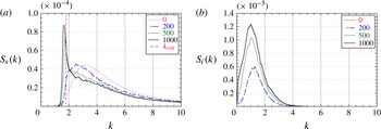
Figure 5 shows the temporal evolution of the spectra
 $S_{s}(k)$
and
 $S_{i}(k)$
. In the figure the spectra are shown only for
 $k>0$
corresponding to the waves propagating in the positive direction. For
 $k<0$
,
 $S_{s}(k)$
and
 $S_{i}(k)$
remain less than
 $4.8\times 10^{-7}$
and
 $6.5\times 10^{-9}$
, respectively, up to
 $1000T_{p}$
, implying that practically no negatively propagating waves have been generated in the course of the evolution.
From figure 5(a), it is clearly observed that
 $S_{s}(k)$
downshifts toward the lower wavenumber, suggesting that there is a significant inverse energy cascade from larger wavenumbers to smaller wavenumbers. However, this downshift halts when the peak of
 $S_{s}(k)$
approaches
 $k\approx 1.8$
, and after that a steep peak appears around
 $k=1.8$
. The spectrum
 $S_{i}(k)$
of the interfacial waves, which is initially zero for all
 $k$
, grows monotonically in the low-wavenumber region around
 $k=1$
as shown in figure 5(b). Since the wave field virtually consists only of positively propagating waves throughout the evolution, this growth of
 $S_{i}(k)$
should have been brought about by the class 3 triad resonance.
Evolution of the wavenumber spectra for case 1 (
 $h_{l}=2$
,
 $R=0.8$
,
 $k_{p}=3.5$
) with
 $t=0,200T_{p},500T_{p},1000T_{p}$
: (a) the surface waves; (b) the interfacial waves.

As the resonance curve of figure 3 shows, there is a lower limit for the wavenumber
 $k_{s}$
of the surface wave to participate in a class 3 triad resonance. We call this lower limit the ‘critical wavenumber’ and denote it as
 $k_{crit}$
. When
 $h_{l}=2$
and
 $R=0.8$
,
 $k_{crit}=1.79$
. It is well known from the wave turbulence theory that only the resonant interactions can transfer energy among waves with different wavenumbers in a secular manner, hence can change the shape of the spectrum. The halt of the downshift of
 $S_{s}(k)$
observed in figure 5(a) can be understood as a natural consequence of the fact that below
 $k=1.79$
there is no surface waves which can participate in any class 3 triad resonance.
In the neighbourhood of
 $k_{crit}$
, the difference
 ${\it\delta}k$
between the wavenumbers
 $k_{s1}$
,
 $k_{s2}$
of the two surface waves in a resonant triad becomes very small (
 $k_{s2}=k_{s1}+{\it\delta}k$
). In the limit
 ${\it\delta}k\rightarrow 0$
corresponding to the critical point itself, the class 3 resonance conditions require
 $$\begin{eqnarray}\frac{\text{d}{\it\omega}_{S}(k)}{\text{d}k}=\lim _{{\it\delta}k\rightarrow 0}\frac{{\it\omega}_{I}({\it\delta}k)}{{\it\delta}k},\end{eqnarray}$$
implying that the group velocity of the (short) surface wave coincides with the long-wave limit of the phase velocity of the (long) interfacial wave. This special type of three-wave resonance is known as the ‘long-wave–short-wave resonance’ (see, for example, Benney Reference Benney1976, Reference Benney1977; Funakoshi & Oikawa Reference Funakoshi and Oikawa1983). The importance of this long-wave–short-wave resonance will be discussed in § 6.
For case 2 with
 $h_{l}=0.5$
,
 $R=0.8$
,
 $k_{p}=3.5$
and
 $A=1.5\times 10^{-4}$
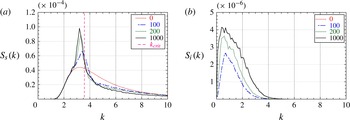
, the temporal evolution of the spectra
 $S_{s}(k)$
and
 $S_{i}(k)$
are shown in figure 6. For the combination of
 $h_{l}$
and
 $R$
of this case,
 $k_{crit}=3.58$
and is in the central part of
 $S_{s}(k)$
at
 $t=0$
. In case 1 discussed above, there is no significant energy around
 $k_{crit}$
initially, and the formation of the sharp peak starts after such a long time as several hundreds of periods have elapsed, during which an appreciable amount of energy is transferred to the region around
 $k_{crit}$
. However in case 2, there exist a sufficient amount of energy around
 $k_{crit}$
from the outset, and the formation of a sharp peak starts from the very beginning of the evolution. The amount of energy present in the range
 $k>k_{crit}$
decreases considerably in order to counterbalance the growth of the peak around
 $k_{crit}$
just like we observed in case 1.
The same as figure 5 for case 2 (
 $h_{l}=0.5$
,
 $R=0.8$
,
 $k_{p}=3.5$
) with
 $t=0,100T_{p},200T_{p},1000T_{p}$
.

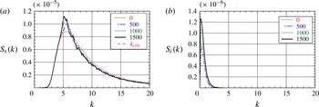
The same as figure 5 for case 3 (
 $h_{l}=\infty$
,
 $R=0.95$
,
 $k_{p}=6.0$
) with
 $t=0,500T_{p},1000T_{p},1500T_{p}$
.

Lastly we studied case 3 where
 $h_{l}=\infty$
,
 $R=0.95$
as a model of the real oceans. By supposing that the depth of the thermocline is some 200 m and that the characteristic wavelength of the ocean surface waves is also around 200 m, we set
 $k_{p}=6.0$
. (Remember that the depth of the upper layer
 $h_{l}=1$
according to our normalization.) The parameter
 $A$
in the initial spectrum (4.1) is chosen as
 $A=3.0\times 10^{-5}$
, which corresponds to
 $ak_{s}=0.072$
.
Figure 7 shows the temporal evolution of the spectra
 $S_{s}(k)$
and
 $S_{i}(k)$
up to
 $t=1500T_{p}$
. When
 $h_{l}=\infty$
, the condition (5.1) for the long-wave–short-wave resonance reduces to
 $k_{crit}=1/4(1-R)$
, giving
 $k_{crit}=5$
for
 $R=0.95$
. This case is similar to case 2 in the sense that
 $k_{crit}$
is in the midst of the initial spectrum
 $S_{s}(k)$
. However, as can be seen in figure 7(a), the evolution of
 $S_{s}(k)$
as a whole, including the formation of a sharp peak, seem much slower than case 2. It can also be noticed in figure 7(b) that the wavenumber of the generated interfacial waves are confined to a much narrower range located at smaller wavenumbers than in the previous two cases. We should await further studies with many other different parameter settings for any definite conclusion, but judging from the result shown here the interaction between surface and interfacial waves may have only a limited effect on the evolution of
 $S_{s}(k)$
in the realistic ocean conditions.
6. Conclusions and discussion
6.1. Conclusions
The results obtained in this work can be summarized as follows.
We have developed a numerical code which simulates the wave motion in a two-layer fluid system based on the HOS method. The nonlinearity is considered up to the second order in the amplitude, and the waves are assumed to propagate in one dimension. We confirmed the validity of the numerical code by reproducing the growth of the amplitudes of a triad of waves which are in a class 3 resonance. We found a good quantitative agreement between the numerical results and the theoretical predictions obtained by the multiple timescale analysis.
With regard to the spectral evolution of a random wave field with a broadband spectrum, we have investigated three cases with different parameter settings. For case 1 with
 $h_{l}=2$
and
 $R=0.8$
, the critical wavenumber
 $k_{crit}=1.79$
and is well below the bulk of the initial surface wave spectrum
 $S_{s}(k)$
when
 $k_{p}=3.5$
. Then
 $S_{s}(k)$
downshifts to a lower wavenumber region during the initial stage of the evolution. However, this downshift halts around the time when the peak of
 $S_{s}(k)$
crosses
 $k_{crit}$
, from then on
 $S_{s}(k)$
gets more and more peaky around
 $k_{crit}$
. For case 2 with
 $h_{l}=0.5$
and
 $R=0.8$
,
 $k_{crit}=3.58$
and is in the midst of the initial
 $S_{s}(k)$
when
 $k_{p}=3.5$
. Then the peak wavenumber of
 $S_{s}(k)$
remains almost the same, and the formation of a sharp peak in
 $S_{s}(k)$
around
 $k_{crit}$
starts from the very beginning of the spectral evolution. For case 3 with
 $h_{l}=\infty$
and
 $R=0.95$
,
 $k_{crit}=5$
and is again close to the peak wavenumber of the initial
 $S_{s}(k)$
when
 $k_{p}=6$
. A sharp peak in
 $S_{s}(k)$
grows around
 $k_{crit}$
from the outset. The energy used for this growth of a peak is supplied from the larger-wavenumber region with
 $k>k_{crit}$
. In every case that we have studied, the interfacial wave spectrum
 $S_{i}(k)$
showed a monotonic growth in a narrow band of a small-wavenumber region.
Even in case 1, in which the energy transfer from the surface waves to the interfacial waves is most vigorous among the three cases reported here, the amount of energy which has been transferred from the surface waves to the interfacial waves is less than 10 % of the total energy contained in the wave field during the evolution up to
 $t=1000T_{p}$
. Therefore, the interfacial waves may not be significant as far as the energy budget among surface and interfacial waves is concerned. However, the existence of these energetically insignificant interfacial waves has a remarkable ability to significantly change the shape of the surface wave spectrum
 $S_{s}(k)$
. Remember that if there is no density interface and the interfacial waves are not allowed to exist,
 $S_{s}(k)$
cannot change at all in this order of nonlinearity.
6.2. Discussion
6.2.1. Kinetic equation
We observed in case 1 that
 $S_{s}(k)$
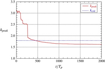
downshifts toward smaller wavenumbers in the initial stage of the spectral evolution prior to the formation of a sharp peak. Figure 8 shows the wavenumber
 $k_{peak}$
where
 $S_{s}(k)$
takes the maximum as a function of time up to
 $t=2000T_{p}$
. It can be observed that
 $k_{peak}$
decreases rapidly during the first 200–300 periods, but remains almost constant after
 $500T_{p}$
. Note that
 $k_{peak}$
decreases even beyond
 $k_{crit}~(=1.79)$
.
The change in time of the peak wavenumber
 $k_{peak}$
of
 $S_{s}(k)$
(case 1,
 $k_{crit}=1.79$
).

Closeup of the evolution of
 $S_{s}(k)$
around
 $k_{crit}$
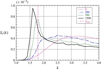
with
 $t=0,200T_{p},500T_{p},1500T_{p}$
(case 1,
 $k_{crit}=1.79$
).

Provided that the system is described as a Hamiltonian system as
 $$\begin{eqnarray}\text{i}\frac{\partial A_{k}}{\partial t}=\frac{{\it\delta}H}{{\it\delta}A_{k}^{\ast }},\quad \text{i}\frac{\partial B_{k}}{\partial t}=\frac{{\it\delta}H}{{\it\delta}B_{k}^{\ast }},\quad H=H_{2}+H_{3},\end{eqnarray}$$
with
 $$\begin{eqnarray}\displaystyle & \displaystyle H_{2}=\int ({\it\omega}_{k}|A_{k}|^{2}+{\it\sigma}_{k}|B_{k}|^{2})\text{d}k, & \displaystyle\end{eqnarray}$$
 $$\begin{eqnarray}\displaystyle & \displaystyle H_{3}=\iiint (V_{123}A_{1}^{\ast }A_{2}B_{3}+\text{c.c.}){\it\delta}(k_{1}-k_{2}-k_{3})\text{d}k_{123}. & \displaystyle\end{eqnarray}$$
 $A_{k}$
and
 $B_{k}$
are the ‘canonical’ amplitudes of the surface wave and the interfacial wave, respectively, and
 ${\it\omega}_{k}$
and
 ${\it\sigma}_{k}$
are the linear frequency of the surface wave and the interfacial wave, respectively. The kernel
 $V_{123}$
is a complicated function of
 $k_{1}$
,
 $k_{2}$
and
 $k_{3}$
. If the amplitude equations (3.4) of a resonant triad were written in terms of these canonical amplitudes instead of the amplitudes
 $a_{k}$
of the surface displacement
 ${\it\eta}_{s}$
, all three coefficients
 ${\it\gamma}$
would take the same value given by
 $-V(k_{s2},k_{s1},k_{i})$
.
Applying the standard procedure of the wave turbulence theory (Zakharov et al. Reference Zakharov, L’vov and Falkovich1992; Nazarenko Reference Nazarenko2011) to (6.1), we obtain the following kinetic equations:
 $$\begin{eqnarray}\displaystyle \frac{\text{d}n_{k}}{\text{d}t} & = & \displaystyle -2{\rm\pi}\iint \left[|V_{k12}|^{2}\{(n_{k}-n_{1})N_{2}+n_{k}n_{1}\}{\it\delta}({\it\omega}_{k}-{\it\omega}_{1}-{\it\sigma}_{2}){\it\delta}(k-k_{1}-k_{2})\text{d}k_{1,2}\right.\nonumber\\ \displaystyle & & \displaystyle \left.-\,|V_{1k2}|^{2}\{(n_{1}-n_{k})N_{2}+n_{k}n_{1}\}{\it\delta}({\it\omega}_{k}-{\it\omega}_{1}+{\it\sigma}_{2}){\it\delta}(k-k_{1}+k_{2})\text{d}k_{1,2}\right],\end{eqnarray}$$
 $$\begin{eqnarray}\displaystyle \frac{\text{d}N_{k}}{\text{d}t} & = & \displaystyle 2{\rm\pi}\iint |V_{12k}|^{2}\{n_{1}N_{k}-n_{2}N_{k}+n_{1}n_{2}\}{\it\delta}({\it\sigma}_{k}-{\it\omega}_{1}+{\it\omega}_{2}){\it\delta}(k-k_{1}+k_{2})\text{d}k_{1,2},\qquad\end{eqnarray}$$
 $n_{k}=\langle |A_{k}|^{2}\rangle$
and
 $N_{k}=\langle |B_{k}|^{2}\rangle$
are the action densities of the surface and the interfacial waves, respectively, and are related to
 $S_{k}(k)$
and
 $S_{i}(k)$
as
 $n_{k}=S_{s}(k)/{\it\omega}_{k}$
and
 $N_{k}=S_{i}(k)/{\it\sigma}_{k}$
, respectively. The existence of two delta functions in (6.3), one for
 $k$
and one for
 ${\it\omega}$
, implies that the changes of the spectra would be governed exclusively by the resonant interactions. Thus, the wave turbulence theory predicts that
 $S_{s}(k)$
would not change in the range
 $k<k_{crit}$
. However, as shown in figure 8 the peak of
 $S_{s}(k)$
clearly downshifts beyond
 $k_{crit}$
. Figure 9 is a closeup of the temporal change of
 $S_{s}(k)$
around
 $k_{crit}$
. It is apparent that
 $S_{s}(k)$
changes significantly even in the range
 $k<k_{crit}$
.
6.2.2. Timescale of the spectral evolution
In order to investigate this apparent discrepancy between the prediction of the wave turbulence theory and the results of the numerical simulation, we check the timescale of the spectral evolution. If (6.3) actually governs the evolution of
 $S_{s}(k)$
and
 $S_{i}(k)$
, the normalized spectra
 $\tilde{S}_{s}(k)\equiv S_{s}(k)/A$
and
 $\tilde{S}_{i}(k)\equiv S_{i}(k)/A$
should be a function of the scaled time
 ${\it\tau}\equiv At$
, where
 $A$
is the multiplicative coefficient of the initial
 $S_{s}(k)$
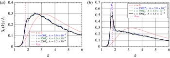
as in (4.1) which controls the degree of nonlinearity of the wave field as a whole. Figure 10 plots
 $\tilde{S}_{s}(k)$
obtained from the numerical simulations for case 1 (
 $h_{l}=2$
,
 $R=0.8$
,
 $k_{p}=3.5$
) with three different values of
 $A$
. Figure 10(a) shows
 $\tilde{S}_{s}(k)$
for three different combinations
 $(A,t)=(0.5\times 10^{-4},600T_{p})$
, (
 $1.0\times 10^{-4}$
,
 $300T_{p}$
), and (
 $1.5\times 10^{-4}$
,
 $200T_{p}$
), all corresponding to
 ${\it\tau}=3.0\times 10^{-2}$
. Furthermore they all belong to the initial stage of spectral evolution prior to the formation of a sharp peak in
 $S_{s}(k)$
. It can be clearly observed that the three scaled spectra nicely coincide with each other, implying that the timescale of the spectral evolution is consistent with (6.3), hence with the wave turbulence theory.
Figure 10(b) is the same as figure 10(a) except for the value of
 ${\it\tau}$
. In the figure
 $\tilde{S}_{s}(k)$
are shown for
 $(A,t)=(0.5\times 10^{-4},1500T_{p})$
,
 $(1.0\times 10^{-4},750T_{p})$
and (
 $1.5\times 10^{-4}$
,
 $500T_{p}$
), all corresponding to
 ${\it\tau}=7.5\times 10^{-2}$
. These combinations of
 $A$
and
 $t$
belong to the later stage of the spectral evolution, and a remarkable peak has already been established in
 $S_{s}(k)$
around
 $k_{crit}$
. Although we can see again a satisfactory coincidence of the three plots in most range of
 $k$
, nevertheless the discrepancy around the sharp peak, i.e. around
 $k_{crit}$
is remarkable. This discrepancy strongly indicates that the formation of the sharp peak in
 $S_{s}(k)$
cannot be explained within the framework of the wave turbulence theory. If we look at the discrepancy between the three plots of
 $\tilde{S}_{s}(k)$
closely, we note that the growth of the peak in
 $\tilde{S}_{s}(k)$
is slower when
 $A$
is larger. This implies that the formation of the peak is dictated by a mechanism whose timescale is faster than
 $O(1/{\it\epsilon}^{2})$
, i.e. the timescale of the spectral evolution predicted by the wave turbulence theory, where
 ${\it\epsilon}$
being the typical non-dimensional amplitude and
 ${\it\epsilon}\propto \sqrt{A}$
.
Normalized spectrum
 $\tilde{S}_{s}(k)$
of surface waves for different sets of
 $(A,t)$
corresponding to the same value of the scaled time
 ${\it\tau}$
(case 1:
 $h_{l}=2$
,
 $R=0.8$
,
 $k_{p}=3.5$
): (a)
 ${\it\tau}=3\times 10^{-2}$
; (b)
 ${\it\tau}=7.5\times 10^{-2}$
.

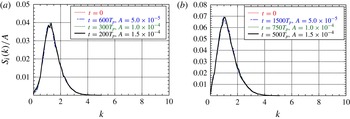
Figure 11 is the same as figure 10 but for the scaled interfacial waves spectrum
 $\tilde{S}_{i}(k)$
instead of
 $\tilde{S}_{s}(k)$
. It is interesting or even puzzling that the timescale of the evolution of
 $S_{i}(k)$
remains perfectly consistent with that predicted by the wave turbulence theory not only in the initial stage (a) but also in the later stage (b) when a remarkable peak has already been formed in
 $S_{s}(k)$
and the wave turbulence scaling has been broken for
 $S_{s}(k)$
particularly around
 $k_{crit}$
as shown in figure 10(b).
The same as figure 10 for the normalized spectrum
 $\tilde{S}_{i}(k)$
of interfacial waves: (a)
 ${\it\tau}=3\times 10^{-2}$
; (b)
 ${\it\tau}=7.5\times 10^{-2}$
.

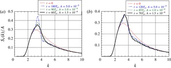
Normalized spectrum
 $\tilde{S}_{s}(k)$
of surface waves for different sets of
 $(A,t)$
obtained for case 2: (a)
 $(A,t)$
corresponding to
 ${\it\tau}=9\times 10^{-3}$
; (b)
 $(A,t)$
corresponding to
 $\tilde{{\it\tau}}\approx 0.85$
.

Figure 12 shows the normalized surface wave spectrum
 $\tilde{S}_{s}(k)$
obtained for case 2 with
 $h_{l}=2$
,
 $R=0.8$
,
 $k_{p}=3.5$
. The three plots shown in figure 12(a) are for
 $(A,t)=(0.5\times 10^{-4},180T_{p})$
, (
 $1.0\times 10^{-4}$
,
 $90T_{p}$
), and (
 $1.5\times 10^{-4}$
,
 $60T_{p}$
), all corresponding to the scaled time
 ${\it\tau}=9\times 10^{-3}$
and are expected to become a single curve if their evolution were governed by the kinetic equation (6.3). On the other hand, the three plots shown in figure 12(b) are for
 $(A,t)=(0.5\times 10^{-4},120T_{p})$
, (
 $1.0\times 10^{-4}$
,
 $85T_{p}$
) and (
 $1.5\times 10^{-4}$
,
 $70T_{p}$
), and all correspond to almost the same value of another scaled time
 $\tilde{{\it\tau}}$
defined by
 $\tilde{{\it\tau}}=\sqrt{A}\,t$
, i.e.
 $\tilde{{\it\tau}}\approx 0.85$
. Figure 12(a) shows that the bulk of the spectrum, except for the region around
 $k_{crit}~(=3.58)$
, is evolving in time with the typical timescale of
 $O(1/A)$
(or
 $O(1/{\it\epsilon}^{2})$
) consistent with the wave turbulence theory. As figure 12(b) shows, on the other hand, the typical timescale of the formation and growth of the sharp peak of
 $S_{s}(k)$
is
 $O(1/\sqrt{A})$
(or
 $O(1/{\it\epsilon})$
) instead of
 $O(1/A)$
. The timescale
 $O(1/{\it\epsilon})$
is that of a deterministic three-wave process such as that described by (3.4), and is much faster than that of the stochastic three-wave process represented by the kinetic equation (6.3).
Right at the
 $k_{crit}$
there exists a strong deterministic three-wave resonance known as the long-wave–short-wave resonance (Benney Reference Benney1976, Reference Benney1977; Funakoshi & Oikawa Reference Funakoshi and Oikawa1983). In a typical situation, the governing equation for this resonance reads
 $$\begin{eqnarray}\text{i}(S_{t}+c_{g}S_{x})+{\textstyle \frac{1}{2}}{\it\omega}^{\prime \prime }S_{xx}={\it\alpha}SL,\quad (L_{t}+c_{p}L_{x})={\it\beta}(|S|^{2})_{x},\quad c_{g}=c_{p},\end{eqnarray}$$
where
 $S$
is the envelope of the short wave and
 $L$
is the long wave. It is almost certain that the existence of this deterministic long-wave–short-wave resonance at
 $k_{crit}$
inevitably alters the otherwise much slower spectral evolution due to ‘stochastic resonance’ as that described by the kinetic equation (6.3) not only right at
 $k_{crit}$
but also in some neighbourhood of it. Due to the existence of the deterministic quasi-resonance around
 $k_{crit}$
, the randomness of the phases of the component waves, which is the most crucial premise for the wave turbulence theory to hold, may have probably been broken there. However, the type of formulation which leads to (6.4) cannot describe the spectral structure of the surface waves (short waves) and the interfacial waves (long waves) which we have observed in the numerical study. Then it should be worth investigating more extensively what role the long-wave–short-wave resonance plays in the spectral evolution of the random wave field with a broadband spectrum. In any case, the two-layer fluid system studied here is quite an interesting system in the sense that the stochastic three-wave process of the timescale of
 $O(1/{\it\epsilon}^{2})$
and the deterministic three-wave process of the timescale of
 $O(1/{\it\epsilon})$
coexist and that each plays a dominant role in its respective range of the wavenumber space.
It should also be interesting to study the evolution of
 $S_{s}(k)$
and
 $S_{i}(k)$
based on the kinetic equations (6.3) and compare the results with those of the direct numerical simulation of the present paper. At the very initial stage of the evolution,
 $N(k)\approx 0$
and (6.3) is then rewritten as
 $$\begin{eqnarray}\displaystyle \displaystyle \frac{\text{d}n(k)}{\text{d}t} & = & \displaystyle -2{\rm\pi}\frac{|V(k,k_{l},k_{i})|^{2}}{\left|(\text{d}{\it\omega}(k_{l})/\text{d}k)-(\text{d}{\it\sigma}(k_{i})/\text{d}k)\right|}n(k)n(k_{l})\nonumber\\ \displaystyle & & \displaystyle +\,2{\rm\pi}\frac{|V(k_{u},k,k_{i})|^{2}}{\left|(\text{d}{\it\omega}(k_{u})/\text{d}k)-(\text{d}{\it\sigma}(k_{i})/\text{d}k)\right|}n(k)n(k_{u}),\end{eqnarray}$$
 $$\begin{eqnarray}\displaystyle \displaystyle \frac{\text{d}N(k_{i})}{\text{d}t} & = & \displaystyle 2{\rm\pi}\frac{|V(k_{u},k_{l},k_{i})|^{2}}{\left|(\text{d}{\it\omega}(k_{u})/\text{d}k)-(\text{d}{\it\omega}(k_{l})/\text{d}k)\right|}n(k_{u})n(k_{l}),\end{eqnarray}$$
 $k_{l}\,({<}k)$
and
 $k_{i}$
in the first term on the right-hand side of (6.5a
) are the wavenumber of the surface wave and that of the interfacial wave, respectively, such that
 $(k,k_{l},k_{i})$
becomes a resonant triplet, while
 $k_{u}\,({>}k)$
and
 $k_{i}$
in the second term on the right-hand side of (6.5a
) are the wavenumber of the surface wave and that of the interfacial wave, respectively, such that
 $(k,k_{u},k_{i})$
becomes a resonant triplet. The first term of (6.5a
), which is negative definite, gives the contribution from the resonant interaction with the partner surface wave with a smaller wavenumber, while the second term, which is positive definite, gives the contribution from the resonant interaction with the partner surface wave with a larger wavenumber. Thus, this equation clearly indicates that the energy of the surface waves is transferred from larger wavenumbers to smaller wavenumbers, at least during the very initial stage of the evolution when the interfacial wave spectrum
 $N\approx 0$
.
The comparison between the spectra at
 $t=1000T_{p}$
and at
 $t=2000T_{p}$
(case 1:
 $h_{l}=2$
,
 $R=0.8$
,
 $k_{p}=3.5$
): (a)
 $S_{s}(k)$
; (b)
 $S_{i}(k)$
.

So far we have confirmed for case 1, where
 $k_{crit}$
is far away from the centre of the initial spectrum
 $S_{s}(k)$
, that the rate of change of
 $S_{i}(k)$
predicted by (6.5b
) is quite similar to that obtained by the numerical simulation which is estimated from the difference between
 $S_{i}(k)$
at
 $t=50T_{p}$
and
 $t=0$
. The study based on the kinetic equation is still under way, and will be reported elsewhere in the future.
6.2.3. Longer-term evolution of the spectra
We showed above that a sharp peak grows in
 $S_{s}(k)$
around
 $k_{crit}$
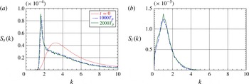
. But this growth does not seem to last forever. Figure 13(a,b) show
 $S_{s}(k)$
and
 $S_{i}(k)$
, respectively, at
 $t=1000T_{p}$
and
 $t=2000T_{p}$
obtained from case 1 with
 $h_{l}=2$
,
 $R=0.8$
. We cannot observe any significant change in either
 $S_{s}(k)$
or
 $S_{i}(k)$
during
 $1000T_{p}$
, and it seems as if the spectra have reached some quasi-equilibrium state. As is clearly seen from the significant change of
 $S_{s}(k)$
and
 $S_{i}(k)$
during
 $t=0$
and
 $t=1000T_{p}$
as shown in figure 5, the duration of
 $1000T_{p}$
is quite a long time for the spectral evolution for the parameters chosen. Our two-layer fluid system is an isolated system, and no artificial source or sink of energy is present in the numerical simulation. It would be quite interesting to investigate whether such an isolated system can ever sustain by itself a stationary spectrum which is different from that corresponding to the energy equipartition. At the moment we do not have enough information on this problem, and further studies are necessary.
Acknowledgement
The authors are grateful to Dr N. Yokoyama for valuable discussions.