2.1 The Boltzmann-BGK equation

It was in 1872 that Ludwig Eduard Boltzmann introduced his famous equation describing the statistical evolution of monatomic gases (Boltzmann Reference Boltzmann1872). The latter accounts for the evolution of the particle distribution function over space, time and a velocity space $f(\boldsymbol{x},t,\unicode[STIX]{x1D743})$. In the absence of body-force terms, the latter reads

(2.1)$$\begin{eqnarray}\frac{\unicode[STIX]{x2202}f}{\unicode[STIX]{x2202}t}+\unicode[STIX]{x1D709}_{\unicode[STIX]{x1D6FC}}\frac{\unicode[STIX]{x2202}f}{\unicode[STIX]{x2202}\unicode[STIX]{x1D6FC}}=\unicode[STIX]{x1D6FA}(\,f),\end{eqnarray}$$

where Einstein’s notation is used for the implicit summation over $\unicode[STIX]{x1D6FC}\in \{x,y,z\}$. On the left-hand side dwells the advective term for the particles moving at velocity $\unicode[STIX]{x1D743}$. On the right-hand side resides collision, modelled as a source term $\unicode[STIX]{x1D6FA}(\,f)$. In general, this collision operator takes a sophisticated form. Assuming the gas to be subject to molecular chaos (Stossansatz), it is possible to express the collision term by considering all possible two-particle interactions (Villani Reference Villani2001):

(2.2)$$\begin{eqnarray}\unicode[STIX]{x1D6FA}(\,f)(\unicode[STIX]{x1D743})=\int _{\unicode[STIX]{x1D743}^{\ast }}\text{d}\unicode[STIX]{x1D743}^{\ast }\int _{\unicode[STIX]{x1D6F4}}B(\unicode[STIX]{x1D6F4},\unicode[STIX]{x1D743}^{\ast })[F(\unicode[STIX]{x1D743},\unicode[STIX]{x1D743}^{\ast },\unicode[STIX]{x1D6F4})-G(\unicode[STIX]{x1D743},\unicode[STIX]{x1D743}^{\ast },\unicode[STIX]{x1D6F4})]\,\text{d}\unicode[STIX]{x1D6F4},\end{eqnarray}$$

where $\unicode[STIX]{x1D743}^{\ast }$ defines the velocity of the second particle, $\unicode[STIX]{x1D6F4}$ the collision angle and $B(\unicode[STIX]{x1D6F4},\unicode[STIX]{x1D743}^{\ast })$ the cross-section of the collision. The functions $F$ and $G$ are related to the probabilities associated with the particles before and after collision. Although general and physical, such a form cannot be easily studied nor implemented for simulation, due to the tremendous cost of computing the integral over all possible velocities and collision angles. For that reason, a simplified collision operator $\unicode[STIX]{x1D6FA}_{BGK}$ known as Bhatnagar–Gross–Krook (BGK) is often introduced (Bhatnagar et al. Reference Bhatnagar, Gross and Krook1954). This term aims at modelling the relaxation of the distribution function $f$ towards an equilibrium $f^{eq}$ over the characteristic time $\unicode[STIX]{x1D70F}$. This simplifies the Boltzmann equation (2.1) to the so-called Boltzmann-BGK equation

(2.3)$$\begin{eqnarray}\frac{\unicode[STIX]{x2202}f}{\unicode[STIX]{x2202}t}+\unicode[STIX]{x1D709}_{\unicode[STIX]{x1D6FC}}\frac{\unicode[STIX]{x2202}f}{\unicode[STIX]{x2202}\unicode[STIX]{x1D6FC}}=\unicode[STIX]{x1D6FA}_{BGK}(\,f)=-\frac{1}{\unicode[STIX]{x1D70F}}(\,f-f^{eq}).\end{eqnarray}$$

In that context, $f^{eq}$ is the well-known Maxwell distribution (Maxwell Reference Maxwell1860):

(2.4)$$\begin{eqnarray}f^{eq}=\frac{\unicode[STIX]{x1D70C}}{(2\unicode[STIX]{x03C0}RT)^{D/2}}\text{e}^{(-(\Vert \unicode[STIX]{x1D743}-\boldsymbol{u}\Vert ^{2})/2RT)},\end{eqnarray}$$

where $D$ is the dimension of space, $T$ the temperature, $R$ the gas constant and $\unicode[STIX]{x1D70C}$ the mass density (the distribution function includes the molecular mass of the particles). Note that this traditional framework is often referred to as thermal, because the temperature $T$ intervenes in the Maxwell distribution. In our statistical context, the macroscopic quantities of mass density $\unicode[STIX]{x1D70C}$, momentum $\boldsymbol{j}$ and total energy $E$ are related to the zeroth-, first- and second-order moments of the distribution function as

(2.5)$$\begin{eqnarray}\displaystyle & \displaystyle \unicode[STIX]{x1D70C}=\int f\,\text{d}\unicode[STIX]{x1D743}, & \displaystyle\end{eqnarray}$$

(2.6)$$\begin{eqnarray}\displaystyle & \displaystyle \boldsymbol{j}=\unicode[STIX]{x1D70C}\boldsymbol{u}=\int \unicode[STIX]{x1D743}\,f\,\text{d}\unicode[STIX]{x1D743}, & \displaystyle\end{eqnarray}$$

(2.7)$$\begin{eqnarray}\displaystyle & \displaystyle \unicode[STIX]{x1D6F1}=2\unicode[STIX]{x1D70C}E=\int \unicode[STIX]{x1D743}\boldsymbol{\cdot }\unicode[STIX]{x1D743}\,f\,\text{d}\unicode[STIX]{x1D743}. & \displaystyle\end{eqnarray}$$

For a monatomic gas of heat constant $DR/2$, the temperature $T$ in (2.4) is defined from the physical definition $\unicode[STIX]{x1D6F1}=\unicode[STIX]{x1D70C}\boldsymbol{u}^{2}+D\unicode[STIX]{x1D70C}RT$. For their part, the equilibrium moments $\unicode[STIX]{x1D70C}^{eq}$, $\boldsymbol{j}^{eq}$ and $\unicode[STIX]{x1D6F1}^{eq}$ are defined similarly by injecting $f^{eq}$ in (2.5)–(2.7). Since we have the exact expression for $f^{eq}$, we can compute directly the integrals, leading to $\unicode[STIX]{x1D70C}^{eq}=\unicode[STIX]{x1D70C}$, $\boldsymbol{j}^{eq}=\boldsymbol{j}$ and $\unicode[STIX]{x1D6F1}^{eq}=\unicode[STIX]{x1D6F1}$. In that context, we have

(2.8a-c)$$\begin{eqnarray}\displaystyle \int \unicode[STIX]{x1D6FA}_{BGK}(\,f)\,\text{d}\unicode[STIX]{x1D743}=0,\quad \int \unicode[STIX]{x1D743}\unicode[STIX]{x1D6FA}_{BGK}(\,f)\,\text{d}\unicode[STIX]{x1D743}=0\quad \text{and}\quad \int \unicode[STIX]{x1D743}\boldsymbol{\cdot }\unicode[STIX]{x1D743}\unicode[STIX]{x1D6FA}_{BGK}(\,f)\,\text{d}\unicode[STIX]{x1D743}=0. & & \displaystyle \nonumber\\ \displaystyle & & \displaystyle\end{eqnarray}$$

In other words, the zeroth-, first- and trace of the second-order raw moments of the distribution function are collision invariants in the thermal framework.

2.2 The athermal hypothesis

The present work does not cover exactly this thermal framework: we make use of the well-known athermal hypothesis (Dellar Reference Dellar2001). It simply consists in setting the temperature $T$ in the Maxwell distribution (2.4) to a constant value $T_{f}$. This widespread modification originated from the LBM community, consequent to the struggle of simple-speed lattices (e.g. D1Q3, D2Q9, D3Q19 and D3Q27) to model a satisfactory energy equation (Shan, Yuan & Chen Reference Shan, Yuan and Chen2006). The fluid temperature will naturally and rapidly relax towards $T_{f}$, so its evolution is not specifically scrutinized. Albeit violating energy conservation, this common framework catches very well the physics of isothermal, weakly compressible flows. This choice is also pedagogical, because the proposed definition for the Knudsen number will be largely simplified in what follows. What is more, a thermal D1Q3 lattice cannot exist since three collision invariants for three discrete velocities would mean no collision at all. Thanks to the athermal hypothesis, there only remains two collision invariants, permitting our theoretical considerations for the D1Q3 lattice

(2.9)$$\begin{eqnarray}\int \unicode[STIX]{x1D743}\boldsymbol{\cdot }\unicode[STIX]{x1D743}\unicode[STIX]{x1D6FA}_{BGK,\;athermal\;case}(\,f)\,\text{d}\unicode[STIX]{x1D743}\neq 0.\end{eqnarray}$$

2.3 Interpreting the Boltzmann-BGK equation

Before introducing the DVBE itself, we link it to the fully continuous Boltzmann equation in the limit of an infinite number of discrete velocities. For that, we make use of the equations on the moments which are space and time differential equations free from the dependence on $\unicode[STIX]{x1D743}$. Let us start from (2.3). Even though it is called ‘the Boltzmann-BGK equation’, it is possible to interpret it as an infinite number of equations in different ways. For instance, each given value of $\unicode[STIX]{x1D743}$ in the velocity space defines a particular partial differential equation in space–time. There is an uncountable number of them, because $\unicode[STIX]{x1D743}$ is a continuous value in a real velocity space. But another approach can be considered. If we assume the distribution function to be close to an exponential form (which is the case for its equilibrium counterpart), then $f\in \mathbb{L}^{\infty }$ and an infinite, but here countable, number of moments of the distribution functions can be computed. We define the raw moments as

(2.10)$$\begin{eqnarray}\displaystyle & \displaystyle \boldsymbol{m}^{(n)}=\int \unicode[STIX]{x1D743}^{n}f\,\text{d}\unicode[STIX]{x1D743}, & \displaystyle\end{eqnarray}$$

(2.11)$$\begin{eqnarray}\displaystyle & \displaystyle \boldsymbol{m}_{eq}^{(n)}=\int \unicode[STIX]{x1D743}^{n}f^{eq}\,\text{d}\unicode[STIX]{x1D743}, & \displaystyle\end{eqnarray}$$

where $\unicode[STIX]{x1D743}^{n}$ denotes the tensor product for various components of the velocity. In one dimension, the bold notations become simply $m^{(n)}$ and $m_{eq}^{(n)}$. In parallel, an infinite number of raw moments of the Boltzmann-BGK equation can be computed

(2.12)$$\begin{eqnarray}\int \unicode[STIX]{x1D743}^{n}\left(\frac{\unicode[STIX]{x2202}f}{\unicode[STIX]{x2202}t}+\unicode[STIX]{x1D709}_{\unicode[STIX]{x1D6FC}}\frac{\unicode[STIX]{x2202}f}{\unicode[STIX]{x2202}\unicode[STIX]{x1D6FC}}=-\frac{1}{\unicode[STIX]{x1D70F}}(\,f-f^{eq})\right)\text{d}\unicode[STIX]{x1D743}.\end{eqnarray}$$

Since the variables $\unicode[STIX]{x1D743}$, $\boldsymbol{x}$ and $t$ are independent, the integral and the space–time derivatives commute. This leads this time to a countable number of space–time equivalent equations on the moments of the distribution function

(2.13)$$\begin{eqnarray}\unicode[STIX]{x2202}_{t}\boldsymbol{m}^{(n)}+\unicode[STIX]{x1D735}\boldsymbol{m}^{(n+1)}=-\frac{1}{\unicode[STIX]{x1D70F}}(\boldsymbol{m}^{(n)}-\boldsymbol{m}_{eq}^{(n)}).\end{eqnarray}$$

The $\mathbb{L}^{\infty }$-hypothesis makes (2.3) and (2.13) equivalent. These equations are interesting for several reasons. The zeroth-, first- and the trace of the second-order moments are related to the macroscopic variables of interest $\unicode[STIX]{x1D70C}$, $\boldsymbol{j}$ and $\unicode[STIX]{x1D6F1}$. As mentioned above and most importantly, this formulation is a shift from an uncountable to countable number of space–time equations. This result is the first ingredient linking the DVBE and the Boltzmann-BGK equation. To understand why, we must define correctly what we mean by DVBE.

2.4 The DVBE: definitions

The DVBE is obtained by selecting a finite set of discrete speeds $(\unicode[STIX]{x1D743}_{\boldsymbol{i}})_{i\in \unicode[STIX]{x27E6}1,V\unicode[STIX]{x27E7}}$ and equilibrium distributions $(\,f_{i}^{eq})_{i\in \unicode[STIX]{x27E6}1,V\unicode[STIX]{x27E7}}$ to solve the $V$ partial differential equations

(2.14)$$\begin{eqnarray}\frac{\unicode[STIX]{x2202}f_{i}}{\unicode[STIX]{x2202}t}+\unicode[STIX]{x1D709}_{i_{\unicode[STIX]{x1D6FC}}}\frac{\unicode[STIX]{x2202}f_{i}}{\unicode[STIX]{x2202}\unicode[STIX]{x1D6FC}}=-\frac{1}{\unicode[STIX]{x1D70F}}(\,f_{i}-f_{i}^{eq}).\end{eqnarray}$$

The set $(\unicode[STIX]{x1D743}_{\boldsymbol{i}})_{i\in \unicode[STIX]{x27E6}1,V\unicode[STIX]{x27E7}}$ is called the lattice. First, it is clear that the solved physics will be driven by the selected $\unicode[STIX]{x1D743}_{\boldsymbol{i}}$ and $f_{i}^{eq}$. What we want to know is, how this discretization in velocity space truncates the physics of the fully continuous Boltzmann-BGK equation. In the continuity of § 2.3 it is possible to locate the influence of this truncation by computing the moments of (2.14) and comparing them to (2.13). Since the distributions are now discrete, the moment integrals must be replaced by sums. We replace in that case the continuous notations by

(2.15a,b)$$\begin{eqnarray}\displaystyle \boldsymbol{m}^{(n)}=\mathop{\sum }_{i=1}^{V}\unicode[STIX]{x1D743}_{\boldsymbol{i}}^{n}f_{i}\quad \text{and}\quad \boldsymbol{m}_{eq}^{(n)}=\mathop{\sum }_{i=1}^{V}\unicode[STIX]{x1D743}_{\boldsymbol{i}}^{n}f_{i}^{eq}. & & \displaystyle\end{eqnarray}$$

So as to fix ideas, we reason in one dimension. From here, the important point is to understand that, with $V$ discrete velocities, it is possible to represent $V$ independent moments and along with them a system very similar to the $V$ first equations of (2.13) – the two differences being:

1. (i) $m^{(V)}$ is a linear combination of all the moments $m^{(n\leqslant V-1)}$ through the so-called lattice closure (Karlin, Chikatamarla & Asinari Reference Karlin, Chikatamarla and Asinari2010). Its gradient in the $V$th equation is not a supplementary unknown.

2. (ii) The equilibrium moments can be arbitrarily chosen. They can of course very well be those of the Maxwell equilibrium, but the choice of $f_{i}^{eq}$ is a priori unrestricted.

2.5 The cascade of moments

The last ingredient to link the fully continuous Boltzmann equation and the DVBE is the so-called cascade of moments. A look at (2.13) shows indeed a dependence of each equation on the next-order moment. The system is infinitely cascaded and does not show independent space–time partial differential equations. It is in fact closed at infinity, and its reduction to a smaller and equivalent set of hydrodynamic variables is exactly the challenge posed by the sixth Hilbert problem (Gorban & Karlin Reference Gorban and Karlin2014). One way among many to recover physics from this infinite cascade is to use a Chapman–Enskog expansion, as presented in appendix A. But whatever the method, the principle is to cut off and model the cascade. Its infinite nature in the Boltzmann continuous case makes it an abhorrent problem. For its part, the DVBE is already closed. In that regard, the discretization process leading to the DVBE can be seen as a particular way of cutting off the cascade. From here, it is clear that pushing $V\rightarrow +\infty$ leads naturally to (2.13) if the equilibrium moments are those of the Maxwell distribution. In other words, the DVBE is a form of truncation of (2.13), changing its hydrodynamic limits. In that context, we now understand how the lattice closure and the choice of the equilibrium impact the equations: they change the modelling of the truncated cascade. The choices made when performing the discretization in velocity space will define certain hydrodynamic limits and stability properties we justly study.

2.6 Discretization in velocity space

We now describe the two most common methods to choose $\unicode[STIX]{x1D743}_{\boldsymbol{i}}$ and $f_{i}^{eq}$. The first one is a moment-matching technique for prescribed velocities, and the second one relies on the Gauss–Hermite quadrature.

2.6.1 Moment-matching technique

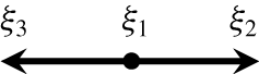
In the general case, it is possible to choose arbitrarily the velocities $\unicode[STIX]{x1D743}_{\boldsymbol{i}}$, and then match given equilibrium moments. Matching those equilibrium moments amounts to a simple matrix problem. We illustrate directly this method with the D1Q3 lattice, as shown in figure 1. We fix $|\unicode[STIX]{x1D709}_{2}|=|\unicode[STIX]{x1D709}_{3}|=r>0$ the norm of two non-zero velocities. Note that the value of $r$ has an influence on the lattice closure. For instance, in our athermal case, we can choose to match the first three equilibrium moments, so that

(2.16)$$\begin{eqnarray}\underbrace{\left(\begin{array}{@{}ccc@{}}1 & 1 & 1\\ 0 & r & -r\\ 0 & r^{2} & r^{2}\end{array}\right)}_{lattice\;choice}\left(\begin{array}{@{}c@{}}f_{1}^{eq}\\ f_{2}^{eq}\\ \,f_{3}^{eq}\end{array}\right)=\underbrace{\left(\begin{array}{@{}c@{}}\unicode[STIX]{x1D70C}\\ \unicode[STIX]{x1D70C}u\\ \unicode[STIX]{x1D70C}u^{2}+\unicode[STIX]{x1D70C}RT_{f}\end{array}\right)}_{equilibrium\;choice}.\end{eqnarray}$$

Since $r>0$, the left-hand side matrix is invertible, and the equilibrium distributions are given by

(2.17)$$\begin{eqnarray}\displaystyle \left.\begin{array}{@{}c@{}}\displaystyle f_{1}^{eq}=\unicode[STIX]{x1D70C}\left[1-\left(\frac{u^{2}+RT_{f}}{r^{2}}\right)\right],\\ \displaystyle f_{2}^{eq}=\frac{\unicode[STIX]{x1D70C}}{2}\left[\frac{u}{r}+\left(\frac{u^{2}+RT_{f}}{r^{2}}\right)\right],\\ \displaystyle f_{3}^{eq}=\frac{\unicode[STIX]{x1D70C}}{2}\left[-\frac{u}{r}+\left(\frac{u^{2}+RT_{f}}{r^{2}}\right)\right].\end{array}\right\} & & \displaystyle\end{eqnarray}$$

This method is general for all lattices, at least when the corresponding left-hand side matrix is invertible. Since the $f_{i}^{eq}$ represent $V$ independent degrees of freedom, it is possible to match up to $V$ independent moments from the Maxwell distribution. The only drawback of the method resides in its lack of generality. A matrix problem must be solved for each lattice: no general expression for $f_{i}^{eq}$ nor the lattice closure are retrieved. The Gauss–Hermite quadrature provides precisely a remedy for these issues.

Figure 1.

Sketch of the D1Q3 lattice.

2.6.2 Gauss–Hermite quadrature

The Gauss–Hermite quadrature is a procedure yielding both $\unicode[STIX]{x1D743}_{\boldsymbol{i}}$ and $f_{i}^{eq}$. The latter makes use of Hermite polynomials $\boldsymbol{{\mathcal{H}}}^{(\boldsymbol{n})}$, as originally proposed by Grad (Reference Grad1949a) and developed thoroughly by Shan et al. (Reference Shan, Yuan and Chen2006). The main interest dwells in their orthogonality properties, regarding a certain scalar product $\langle ,\rangle$. A key point of the Gauss–Hermite procedure is to conserve this property in the discrete case and provide a generic expansion of each $f_{i}^{eq}$ using those particular polynomials – which can be seen as vectors in our finite $V$-dimensional space. But there can only be $V$ different orthogonal vectors, and the so-called quadrature order $Q$ translates this limitation so that

(2.18)$$\begin{eqnarray}\displaystyle \langle \boldsymbol{{\mathcal{H}}}_{a}^{(\boldsymbol{n})},\boldsymbol{{\mathcal{H}}}_{b}^{(\boldsymbol{m})}\rangle =\unicode[STIX]{x1D6FF}_{nm}\unicode[STIX]{x1D6FF}_{ab},\quad \text{for }n+m\leqslant Q, & & \displaystyle\end{eqnarray}$$

where the transcripts $a$ and $b$ identify formally given Hermite polynomials, in the case of several dimensions. For example, if $a\equiv xx$ and $b\equiv xy$, we have $\unicode[STIX]{x1D6FF}_{ab}=0$ and thus $\langle \boldsymbol{{\mathcal{H}}}_{xx}^{(\mathbf{2})},\boldsymbol{{\mathcal{H}}}_{xy}^{(\mathbf{2})}\rangle =0$. In the above equation, the order of quadrature $Q$ is defined as the maximal Hermite polynomial order whose integral can be exactly estimated on the lattice

(2.19)$$\begin{eqnarray}\displaystyle \int w(\unicode[STIX]{x1D743})\boldsymbol{{\mathcal{H}}}^{(\boldsymbol{n})}(\unicode[STIX]{x1D743})\,\text{d}\unicode[STIX]{x1D743}=\mathop{\sum }_{i=1}^{V}w_{i}\,\boldsymbol{{\mathcal{H}}}^{(\boldsymbol{n})}(\unicode[STIX]{x1D743}_{\boldsymbol{i}}),\quad \text{for }n\leqslant Q. & & \displaystyle\end{eqnarray}$$

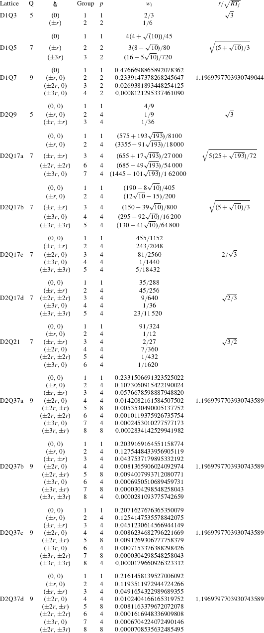
Here, $w$ is the weight function defined in appendix D and $(w_{i})_{i\in \unicode[STIX]{x27E6}1,V\unicode[STIX]{x27E7}}$ are the quadrature weights; $Q$ depends on the choice of the lattice velocities, even though its links with $V$ are intricate. For more details, notably on how (2.19) implies (2.18), the reader can refer to Shan et al. (Reference Shan, Yuan and Chen2006), Philippi et al. (Reference Philippi, Hegele, dos Santos and Surmas2006) or Shan (Reference Shan2016), which provide many examples of lattices. We recall that $Q=5$ for the most famous lattices (D1Q3, D2Q9 and D3Q27, cf. Shan et al. (Reference Shan, Yuan and Chen2006)). In that context, the Gauss–Hermite quadrature provides the following generic truncated expansion on the Hermite basis at a given order $N$:

(2.20)$$\begin{eqnarray}f_{i}^{eq,N}=w_{i}\mathop{\sum }_{n=0}^{N}\boldsymbol{b}_{\boldsymbol{ e}\boldsymbol{q}}^{(\boldsymbol{n})}:\boldsymbol{{\mathcal{H}}}_{\boldsymbol{ i}}^{(\boldsymbol{n})},\end{eqnarray}$$

where $\boldsymbol{{\mathcal{H}}}_{\boldsymbol{i}}=\boldsymbol{{\mathcal{H}}}(\unicode[STIX]{x1D743}_{\boldsymbol{i}})$ and $\boldsymbol{b}_{\boldsymbol{e}\boldsymbol{q}}^{(\boldsymbol{n})}$ are related to the Hermite moments of the equilibrium distribution. More details are given in appendix D. The prescribed recovery of the Hermite moments of the expansion, along with the orthogonality requirement (2.18) imposes de facto $2N\leqslant Q$. This makes the truncation somewhat rough, since it systematically reduces the amount of possible matched moments. For example, with the D2Q9 lattice, the traditional basis arising from the second-order truncation of the equilibrium is

(2.21)$$\begin{eqnarray}({\mathcal{H}}^{(0)},{\mathcal{H}}_{x}^{(1)},{\mathcal{H}}_{y}^{(1)},{\mathcal{H}}_{xx}^{(2)},{\mathcal{H}}_{yy}^{(2)},{\mathcal{H}}_{xy}^{(2)}),\end{eqnarray}$$

which makes six orthogonal vectors for $V=9$ possible ones. Fortunately, it is possible to complete the basis keeping the correct orthogonality properties by adding

(2.22)$$\begin{eqnarray}({\mathcal{H}}_{xxy}^{(3)},{\mathcal{H}}_{yyx}^{(3)},{\mathcal{H}}_{xxyy}^{(4)}).\end{eqnarray}$$

But then, the expansion cannot be expressed under the form (2.20), somewhat limiting the expected degree of generality when recovering all the Maxwell moments. Note that, once the set of velocities fixed, completing the orthogonal basis leads to the same discrete equilibrium distributions $f_{i}^{eq}$ as with moment matching. As a concluding remark, note further that the quadrature order $Q$ is related by definition to the number of recovered Maxwell moments through $N$ in (2.20). As seen in § 2.5 its increase leads to a higher-order cutoff of the cascade of moments. Therefore, the higher $Q$, the better the modelling of the fully continuous Boltzmann-BGK equation.

2.7 Framework of the perturbative analysis

The DVBE forms a set of $V$ coupled equations, whose natural descriptive variables are the discrete distributions $(\,f_{i})_{i\in \unicode[STIX]{x27E6}1,V\unicode[STIX]{x27E7}}$. The perturbative analysis we now perform consists first in setting these distribution functions to a mean field plus a complex wave perturbation as

(2.23)$$\begin{eqnarray}f_{i}=\overline{f_{i}}+\hat{f_{i}}\text{e}^{\text{i}(\unicode[STIX]{x1D714}t-\boldsymbol{k}\boldsymbol{\cdot }\boldsymbol{x})}.\end{eqnarray}$$

The pulsation (also called the angular velocity, or eigenvalue) $\unicode[STIX]{x1D714}$ is assumed to be complex a priori, while the wavevector $\boldsymbol{k}$ is kept real. Note that the exponential is nothing other but a mathematical tool to diagonalize the set of equations. This expression (2.23) is injected in the DVBE (2.14). Simultaneously, a linearization process is performed, which consists simply in keeping only the first orders of $\hat{f_{i}}$. That way, the results can be generalized to any signal in the linear regime thanks to the superposition principle. Assuming that the mean field verifies the equations, this calculation yields two sets of independent relations. One concerns the mean field, the other the perturbations. The first reads

(2.24)$$\begin{eqnarray}\frac{\unicode[STIX]{x2202}\overline{f_{i}}}{\unicode[STIX]{x2202}t}+\unicode[STIX]{x1D709}_{i_{\unicode[STIX]{x1D6FC}}}\frac{\unicode[STIX]{x2202}\overline{f_{i}}}{\unicode[STIX]{x2202}\unicode[STIX]{x1D6FC}}=-\frac{1}{\unicode[STIX]{x1D70F}}(\,\overline{f_{i}}-\overline{f_{i}^{eq}}).\end{eqnarray}$$

Since the variations in space and time of the mean field are null by definition, this equation boils down to

(2.25)$$\begin{eqnarray}\overline{f_{i}}=\overline{f_{i}^{eq}}.\end{eqnarray}$$

The studied mean field is in fact the equilibrium mean field. Thus, the terms $\hat{f_{i}}\text{e}^{\text{i}(\unicode[STIX]{x1D714}t-k_{\unicode[STIX]{x1D6FC}}x_{\unicode[STIX]{x1D6FC}})}$ can be regarded as linear perturbations from the equilibrium state. The second relation concerns the perturbative physics

(2.26)$$\begin{eqnarray}((\text{i}\unicode[STIX]{x1D714}_{\unicode[STIX]{x1D70F}}+1)\mathbb{I}-\text{i}\boldsymbol{{\mathcal{K}}}-\boldsymbol{{\mathcal{J}}}_{eq}(\overline{\boldsymbol{{\mathcal{F}}}}))\widehat{\boldsymbol{{\mathcal{F}}}}=0,\end{eqnarray}$$

where we introduced the column vector of the perturbations

(2.27)$$\begin{eqnarray}\widehat{\boldsymbol{{\mathcal{F}}}}=\left(\begin{array}{@{}c@{}}\hat{f_{1}}\\ \hat{f_{2}}\\ \vdots \\ \,\hat{f_{V}}\end{array}\right).\end{eqnarray}$$

The mean field similarly reads $\overline{\boldsymbol{{\mathcal{F}}}}=(\,\overline{f_{i}})_{i\in \unicode[STIX]{x27E6}1,V\unicode[STIX]{x27E7}}$. The dimensionless pulsation is defined by

(2.28)$$\begin{eqnarray}\unicode[STIX]{x1D714}_{\unicode[STIX]{x1D70F}}=\unicode[STIX]{x1D714}\unicode[STIX]{x1D70F}.\end{eqnarray}$$

The diagonal matrix containing wavevectors coming from the spatial derivatives reads

(2.29)$$\begin{eqnarray}\boldsymbol{{\mathcal{K}}}=\left(\begin{array}{@{}cccc@{}}\unicode[STIX]{x1D70F}\boldsymbol{k}\boldsymbol{\cdot }\unicode[STIX]{x1D743}_{\mathbf{1}} & & & \\ & \unicode[STIX]{x1D70F}\boldsymbol{k}\boldsymbol{\cdot }\unicode[STIX]{x1D743}_{\mathbf{2}} & & \\ & & \ddots & \\ & & & \unicode[STIX]{x1D70F}\boldsymbol{k}\boldsymbol{\cdot }\unicode[STIX]{x1D743}_{\boldsymbol{V}}\\ \end{array}\right).\end{eqnarray}$$

Eventually, the Jacobian matrix of the equilibrium distributions is given by

(2.30)$$\begin{eqnarray}\boldsymbol{{\mathcal{J}}}_{eq}(\overline{\boldsymbol{{\mathcal{F}}}})=\left(\begin{array}{@{}cccc@{}}\displaystyle \frac{\unicode[STIX]{x2202}f_{1}^{eq}}{\unicode[STIX]{x2202}f_{1}} & \displaystyle \frac{\unicode[STIX]{x2202}f_{1}^{eq}}{\unicode[STIX]{x2202}f_{2}} & \ldots \, & \displaystyle \frac{\unicode[STIX]{x2202}f_{1}^{eq}}{\unicode[STIX]{x2202}f_{V}}\\ \displaystyle \frac{\unicode[STIX]{x2202}f_{2}^{eq}}{\unicode[STIX]{x2202}f_{1}} & \displaystyle \frac{\unicode[STIX]{x2202}f_{2}^{eq}}{\unicode[STIX]{x2202}f_{2}} & & \\ \vdots & & \ddots & \\ \displaystyle \frac{\unicode[STIX]{x2202}f_{V}^{eq}}{\unicode[STIX]{x2202}f_{1}} & & & \displaystyle \frac{\unicode[STIX]{x2202}f_{V}^{eq}}{\unicode[STIX]{x2202}f_{V}}\end{array}\right),\end{eqnarray}$$

where all derivatives are evaluated at the mean field $\overline{\boldsymbol{{\mathcal{F}}}}$. We now explain how the matrix $\boldsymbol{{\mathcal{K}}}$ drives the values of $\unicode[STIX]{x1D714}_{\unicode[STIX]{x1D70F}}$ for a given DVBE and mean field in (2.26). By looking more closely at the form (2.29), it is clear that the $V$ products $\unicode[STIX]{x1D70F}\boldsymbol{k}\boldsymbol{\cdot }\unicode[STIX]{x1D743}_{\boldsymbol{i}}$ suffice to determine the solutions of (2.26). Mindful that the velocities $\unicode[STIX]{x1D709}_{i}$ are often of the order $\sqrt{RT_{f}}=c$, dimensionless lattice velocities are introduced

(2.31)$$\begin{eqnarray}e_{i_{\unicode[STIX]{x1D6FC}}}=\frac{\unicode[STIX]{x1D709}_{i_{\unicode[STIX]{x1D6FC}}}}{\sqrt{RT_{f}}}=\frac{\unicode[STIX]{x1D709}_{i_{\unicode[STIX]{x1D6FC}}}}{c},\end{eqnarray}$$

along with a dimensionless wavevector

(2.32)$$\begin{eqnarray}\boldsymbol{K}\boldsymbol{n}=\unicode[STIX]{x1D70F}\boldsymbol{k}\sqrt{RT_{f}}=\unicode[STIX]{x1D70F}\boldsymbol{k}c.\end{eqnarray}$$

Another key point of the present theory dwells here; this dimensionless wavevector can in fact be interpreted as a multi-dimensional generalization of a Knudsen number. We call it here the Knudsen vector $\boldsymbol{K}\boldsymbol{n}$. In that context, the matrix (2.29) can be rewritten using the canonical scalar products between the dimensionless velocities and the Knudsen vector

(2.33)$$\begin{eqnarray}\boldsymbol{{\mathcal{K}}}=\left(\begin{array}{@{}cccc@{}}\boldsymbol{e}_{\mathbf{1}}\boldsymbol{\cdot }\boldsymbol{K}\boldsymbol{n} & & & \\ & \boldsymbol{e}_{\mathbf{2}}\boldsymbol{\cdot }\boldsymbol{K}\boldsymbol{n} & & \\ & & \ddots & \\ & & & \boldsymbol{e}_{\boldsymbol{V}}\boldsymbol{\cdot }\boldsymbol{K}\boldsymbol{n}\\ \end{array}\right).\end{eqnarray}$$

That way, the Knudsen vector stands as a natural descriptive parameter to determine fully the linear (perturbative) physics of the DVBE, for a given mean field. We now justify physically this definition for $\boldsymbol{K}\boldsymbol{n}$.

2.8 The Knudsen number

Introduced by Martin Knudsen a century ago, the Knudsen number is a local dimensionless number defined as the ratio between the free mean path of the particles $l_{FMP}$ and a characteristic length of a perturbation $l_{p}$ in a given fluid

(2.34)$$\begin{eqnarray}Kn=\frac{l_{FMP}}{l_{p}}.\end{eqnarray}$$

The value of $Kn$ defines whether the medium can be considered continuous or if it should be treated statistically as a rarefied fluid. In some measure, the Knudsen number can be regarded as a sampling indicator checking if the perturbation under consideration can be represented continuously by particles, thus by continuous and well-defined macroscopic variables. The continuous condition is fundamental, since the Navier–Stokes modelling is based upon this assumption. Traditionally, the following ranges are given to sort out the various regimes (see Bird & Brady Reference Bird and Brady1994):

1. (i) $Kn\lesssim 0.001$: the medium is fully continuous;

2. (ii) $0.001\lesssim Kn\lesssim 0.1-1$: the medium is almost continuous;

3. (iii) $Kn\gtrsim 1$: the medium is not continuous.

The free mean path $l_{FMP}$ is a well-defined notion in fluid statistics and depends only on the temperature (see Laurendeau Reference Laurendeau2005). It can be regarded as a collision time $\unicode[STIX]{x1D70F}$ multiplied by a quadratic mean speed ${\sim}\sqrt{RT_{f}}$, so we define

(2.35)$$\begin{eqnarray}l_{FMP}=\unicode[STIX]{x1D70F}\sqrt{RT_{f}}.\end{eqnarray}$$

On the other hand, the characteristic length of a perturbation of a quantity $X$ can be derived locally from its gradient as

(2.36)$$\begin{eqnarray}l_{p}\sim \frac{|X|}{|\unicode[STIX]{x1D735}X|}.\end{eqnarray}$$

Within the framework of our perturbative analysis, the characteristic length becomes

(2.37)$$\begin{eqnarray}l_{p}\sim \frac{1}{k}.\end{eqnarray}$$

That is why naturally we get

(2.38)$$\begin{eqnarray}Kn=\unicode[STIX]{x1D70F}k\sqrt{RT_{f}}=\unicode[STIX]{x1D70F}kc.\end{eqnarray}$$

Note that the retrieval of the von Kármán relation is a supplementary confirmation of the physical validity of this definition

(2.39)$$\begin{eqnarray}Kn=\frac{\left(\displaystyle \frac{U}{c}\right)}{\left(\displaystyle \frac{U}{k\unicode[STIX]{x1D708}}\right)}=\frac{Ma}{Re},\end{eqnarray}$$

where $U$ is a fluid velocity and $\unicode[STIX]{x1D708}=\unicode[STIX]{x1D70F}c^{2}$ is the kinematic viscosity of Boltzmann-BGK gases. Note that, on its own, the Knudsen number does not quantify a shift from the equilibrium distribution. It is because this number – or its vector counterpart – drives the linear perturbative physics shift from equilibrium that its interpretation makes sense.

We also give further comments on the definition (2.38). It is important to keep in mind that there exists no such thing as the Knudsen number of the entire flow; $Kn$ depends both on the fluid model and the perturbation considered. Furthermore, no exterior system length (e.g. a distance between two walls or an object in the flow) directly intervenes to define the Knudsen number. Even for very small systems of size $\unicode[STIX]{x1D716}$, such as can be found in microfluidics, the large Knudsen numbers found can be interpreted by arguing that any perturbation cannot exceed the size $\unicode[STIX]{x1D716}$, thus yielding a minimum wavenumber $1/\unicode[STIX]{x1D716}$. This point of view encompasses traditional definitions of the Knudsen number, for instance in nanoporous media involving the pore diameter (Montessori et al. Reference Montessori, Prestininzi, La Rocca and Succi2015, Reference Montessori, Prestininzi, Rocca, Falcucci, Succi and Kaxiras2016; Falcucci et al. Reference Falcucci, Amati, Krastev, Montessori, Yablonsky and Succi2017) or small channels (Toschi & Succi Reference Toschi and Succi2005).

Now that the DVBE and the Knudsen number are well defined, we present our methodology to interpret the solutions of (2.26) in terms of hydrodynamics and stability.

2.8.1 Methodology: retrieving the physics from $\unicode[STIX]{x1D714}_{\unicode[STIX]{x1D70F}}$

The system (2.26) can be solved in two manners. First, the $V$ solutions $\unicode[STIX]{x1D714}_{\unicode[STIX]{x1D70F}}(\boldsymbol{K}\boldsymbol{n},\overline{\boldsymbol{{\mathcal{F}}}})$ can be obtained by studying the kernel of the matrix multiplying the perturbation vector. The solutions are non-trivially equal to zero when

(2.40)$$\begin{eqnarray}\det ((\text{i}\unicode[STIX]{x1D714}_{\unicode[STIX]{x1D70F}}+1)\mathbb{I}-\text{i}\boldsymbol{{\mathcal{K}}}-\boldsymbol{{\mathcal{J}}}_{eq}(\overline{\boldsymbol{{\mathcal{F}}}}))=0.\end{eqnarray}$$

This obtained equation is often referred to as the dispersion relation of the waves propagating physically. It has the advantage of yielding swiftly the pulsations $\unicode[STIX]{x1D714}_{\unicode[STIX]{x1D70F}}$, but does not provide the associated eigenvectors . So as to retrieve them, it is possible to rewrite (2.26) as a complex eigenvalue equivalent problem

(2.41)$$\begin{eqnarray}(\text{i}\mathbb{I}+\boldsymbol{{\mathcal{K}}}-\text{i}\boldsymbol{{\mathcal{J}}}_{eq}(\overline{\boldsymbol{{\mathcal{F}}}}))\widehat{\boldsymbol{{\mathcal{F}}}}=\unicode[STIX]{x1D714}_{\unicode[STIX]{x1D70F}}\widehat{\boldsymbol{{\mathcal{F}}}}.\end{eqnarray}$$

Whatever the method, we focus in this work on the eigenvalues $\unicode[STIX]{x1D714}_{\unicode[STIX]{x1D70F}}$, which are a sufficient tool to answer the questions raised in the previous introductory sections. For their part, the eigenvectors are only the support of the perturbations. They depend also on $\boldsymbol{K}\boldsymbol{n}$, $\overline{\boldsymbol{{\mathcal{F}}}}$, the lattice and the choice of the collision model, but their study is a separate problem outside of the scope of the proposed objectives. Future work, following Wissocq et al. (Reference Wissocq, Sagaut and Boussuge2019), will investigate these points in detail, including the thermal framework.

The real part of the eigenvalues $\text{Re}(\unicode[STIX]{x1D714}_{\unicode[STIX]{x1D70F}})$ yields the non-dimensional phase $\boldsymbol{v}_{\unicode[STIX]{x1D719}}$ and group $\boldsymbol{v}_{g}$ speeds at the considered Knudsen vector $\boldsymbol{K}\boldsymbol{n}$ (or, equivalently, wavevector $\boldsymbol{k}$)

(2.42)$$\begin{eqnarray}\displaystyle & \displaystyle \left.v_{\unicode[STIX]{x1D719}_{\unicode[STIX]{x1D6FC}}}=\frac{\text{Re}(\unicode[STIX]{x1D714}_{\unicode[STIX]{x1D70F}})}{Kn_{\unicode[STIX]{x1D6FC}}}\right|_{\boldsymbol{K}\boldsymbol{n}}, & \displaystyle\end{eqnarray}$$

(2.43)$$\begin{eqnarray}\displaystyle & \displaystyle \left.v_{g_{\unicode[STIX]{x1D6FC}}}=\frac{\unicode[STIX]{x2202}\text{Re}(\unicode[STIX]{x1D714}_{\unicode[STIX]{x1D70F}})}{\unicode[STIX]{x2202}Kn_{\unicode[STIX]{x1D6FC}}}\right|_{\boldsymbol{K}\boldsymbol{n}}. & \displaystyle\end{eqnarray}$$

On the other hand, the imaginary part $\text{Im}(\unicode[STIX]{x1D714}_{\unicode[STIX]{x1D70F}})$ provides information on the dissipation of the waves in the system. Notably, any Knudsen number and mean flow for which $\text{Im}(\unicode[STIX]{x1D714}_{\unicode[STIX]{x1D70F}}(\boldsymbol{K}\boldsymbol{n},\overline{\boldsymbol{{\mathcal{F}}}}))<0$ points to an instability. Such unstable modes will be investigated both theoretically and numerically. In addition, some particular solutions $\unicode[STIX]{x1D714}_{\unicode[STIX]{x1D70F}}$ can be interpreted physically. For instance, acoustic waves appear naturally in all of our studies. One of the main interests of the method is the following. Assuming the function $\unicode[STIX]{x1D714}_{\unicode[STIX]{x1D70F}}(\boldsymbol{K}\boldsymbol{n},\overline{\boldsymbol{{\mathcal{F}}}})$ to be $\mathbb{C}^{\infty }$ in the components of $\boldsymbol{K}\boldsymbol{n}$ close to the origin, it is absolutely rigorous to expand $\unicode[STIX]{x1D714}_{\unicode[STIX]{x1D70F}}$ in series of the Knudsen vector

(2.44)$$\begin{eqnarray}\unicode[STIX]{x1D714}_{\unicode[STIX]{x1D70F}}(\boldsymbol{K}\boldsymbol{n},\overline{\boldsymbol{{\mathcal{F}}}})=\mathop{\sum }_{j,l,m=0}^{+\infty }\unicode[STIX]{x1D714}_{\unicode[STIX]{x1D70F}_{j,l,m}}(\overline{\boldsymbol{{\mathcal{F}}}})\;Kn_{x}^{\,j}\;Kn_{y}^{l}\;Kn_{z}^{m}.\end{eqnarray}$$

The convergence radius can be discussed case by case. But the form and plots of the solutions will provide us rigorous ranges of validity of the approach. Instead of starting from an ansatz, as the Chapman–Enskog expansion does, we can recover valuable information at each order in Knudsen number with certainty. This important notion of Knudsen order will be used in the rest of the work. Since all of our theoretical calculations are one-dimensional, the expansions will take in practice the simplified form

(2.45)$$\begin{eqnarray}\unicode[STIX]{x1D714}_{\unicode[STIX]{x1D70F}}(Kn,\overline{\boldsymbol{{\mathcal{F}}}})=\mathop{\sum }_{j=0}^{+\infty }\unicode[STIX]{x1D714}_{\unicode[STIX]{x1D70F}_{j}}(\overline{\boldsymbol{{\mathcal{F}}}})\,Kn^{\,j}.\end{eqnarray}$$

The expression of the coefficients $\unicode[STIX]{x1D714}_{\unicode[STIX]{x1D70F}_{j}}(\overline{\boldsymbol{{\mathcal{F}}}})$ varies as a function of the system under study, and of course, the mean flow. Note that, in practice, $\overline{\boldsymbol{{\mathcal{F}}}}$ boils down simply and only to the mean Mach number. For the DVBE, these coefficients are a function of the lattice, the equilibrium, the possible MRT modelling and the expression of the forcing terms. Since similar work can be achieved on Euler, Navier–Stokes and Burnett equations, rigorous comparisons of hydrodynamics and stability between these systems at each Knudsen order is therefore feasible. We must simply compare the coefficients. What is more, the notion of Galilean invariance can be rigorously investigated by looking at the coefficients $\unicode[STIX]{x1D714}_{\unicode[STIX]{x1D70F}_{j}}(\overline{\boldsymbol{{\mathcal{F}}}})$. A dependence of the dissipation $\text{Im}(\unicode[STIX]{x1D714}_{\unicode[STIX]{x1D70F}})$ on the mean flow through $\overline{Ma}$ is intrinsically non-physical, because all waves should dissipate similarly in any referential. Similarly, a diagnostic tool of Galilean variance is to check for the dependence of $v_{g}-\overline{Ma}$ and/or $v_{\unicode[STIX]{x1D719}}-\overline{Ma}$ on the mean flow. This can be seen readily by considering the perturbation in the reference system moving with the mean flow $x_{M}$

(2.46)$$\begin{eqnarray}\frac{x_{M}}{\unicode[STIX]{x1D70F}c}=\frac{x}{\unicode[STIX]{x1D70F}c}+\overline{Ma}\frac{t}{\unicode[STIX]{x1D70F}},\end{eqnarray}$$

giving

(2.47)$$\begin{eqnarray}\text{e}^{\text{i}[(\text{Re}(\unicode[STIX]{x1D714}_{\unicode[STIX]{x1D70F}})-Kn\;\overline{Ma})t/\unicode[STIX]{x1D70F}-Kn\;x_{M}/(\unicode[STIX]{x1D70F}c)]}\text{e}^{-\text{i}\;\text{Im}(\unicode[STIX]{x1D714}_{\unicode[STIX]{x1D70F}})t/\unicode[STIX]{x1D70F}}.\end{eqnarray}$$

In this moving frame, Galilean invariance requires that neither $\text{Im}(\unicode[STIX]{x1D714}_{\unicode[STIX]{x1D70F}})$ nor $\text{Re}(\unicode[STIX]{x1D714}_{\unicode[STIX]{x1D70F}})-Kn\;\overline{Ma}$ should depend on $\overline{Ma}$. Thus, the same goes for $v_{g}-\overline{Ma}$ and $v_{\unicode[STIX]{x1D719}}-\overline{Ma}$ (the condition on $v_{\unicode[STIX]{x1D719}}$ being more restrictive). Finally, we will see in § 5 that it is possible to determine the converged behaviour of the coefficients $\unicode[STIX]{x1D714}_{\unicode[STIX]{x1D70F}_{j}}$ when $V\rightarrow +\infty$ and $N\rightarrow +\infty$, giving insight into the linear physics of the fully continuous Boltzmann-BGK equation by virtue of the introductory analysis (2.3)–(2.5).

2.8.2 Validity of the results in LBM

Being discrete space–time approximations of the DVBE, LBM simulations come along with deviations from the continuous physics. Still, supposing the adopted LB scheme to be convergent, the physics of the LB simulation should converge towards that of the DVBE in the limit of infinitely small space and time steps. If it is true that some shifts of non-hydrodynamic waves can be observed at the origin for stream-and-collide schemes (Lallemand & Luo Reference Lallemand and Luo2000), most of the physics of interest should be acceptably comparable in that limit. We now understand how – it is by using two dimensionless parameters which fit remarkably well the proposed framework.

What is to be understood here is that LBM introduces two new parameters into the problem: $\unicode[STIX]{x0394}t$ and $\unicode[STIX]{x0394}x$ (we restrict ourselves to schemes of regular time and space steps). This means that two supplementary dimensionless parameters are necessary for the description of the solutions. One natural parameter is the reduced collision time

(2.48)$$\begin{eqnarray}\unicode[STIX]{x1D70F}/\unicode[STIX]{x0394}t=\unicode[STIX]{x1D70F}_{dimensionless}.\end{eqnarray}$$

The other interesting one, that we introduce here, is the Knudsen–Shannon number. Working on a discrete grid, the Nyquist–Shannon sampling condition must be indeed accounted for (Nyquist Reference Nyquist1928; Shannon Reference Shannon1949). Only the wavenumbers fulfilling

(2.49)$$\begin{eqnarray}k\unicode[STIX]{x0394}x\leqslant \unicode[STIX]{x03C0}\end{eqnarray}$$

can be represented in the simulation. In terms of Knudsen number, this expression can be recast

(2.50)$$\begin{eqnarray}Kn=\unicode[STIX]{x1D70F}kc\leqslant \frac{\unicode[STIX]{x1D70F}c\unicode[STIX]{x03C0}}{\unicode[STIX]{x0394}x}=Kn_{s}.\end{eqnarray}$$

The Knudsen–Shannon number $Kn_{s}$ represents the ultimately represented Knudsen number in the simulation. These two dimensionless parameters have separate effects. Let us for example consider a fixed physical collision time $\unicode[STIX]{x1D70F}$. Then, $\unicode[STIX]{x1D70F}_{dimensionless}$ defines the temporal precision of the scheme, while $Kn_{s}$ defines the spatial precision. But more importantly, considering the expansion (2.45), $Kn_{s}$ defines which orders in Knudsen number must be taken into account in such expansions (it is still possible to compute the waves of LBM and expand the eigenvalues in $Kn$ as before). In the limit $\unicode[STIX]{x1D70F}_{dimensionless}\rightarrow \infty$ and $Kn_{s}\rightarrow \infty$, which is equivalent to infinitely small time and space steps, the physics of the waves of LBM and DVBE should fit and all the Knudsen orders of the expansion can be represented.

In the particular yet extensively used case of stream-and-collide schemes, space and time steps are linked together through an acoustic scaling relation which takes the following general form:

(2.51)$$\begin{eqnarray}\frac{\unicode[STIX]{x0394}x}{\unicode[STIX]{x0394}t}=\unicode[STIX]{x1D70E}c=\unicode[STIX]{x1D70E}\sqrt{RT_{f}},\end{eqnarray}$$

where $\unicode[STIX]{x1D70E}$ is a scaling coefficient which depends on the lattice. In that case, the Knudsen–Shannon number is directly linked to both $\unicode[STIX]{x0394}x$ and $\unicode[STIX]{x0394}t$

(2.52)$$\begin{eqnarray}Kn_{s}=\frac{\unicode[STIX]{x1D70F}c\unicode[STIX]{x03C0}}{\unicode[STIX]{x0394}x}=\frac{\unicode[STIX]{x1D70F}\unicode[STIX]{x03C0}}{\unicode[STIX]{x1D70E}\unicode[STIX]{x0394}t}=\frac{\unicode[STIX]{x03C0}}{\unicode[STIX]{x1D70E}}\unicode[STIX]{x1D70F}_{dimensionless}.\end{eqnarray}$$

The Knudsen–Shannon number and the reduced collision time are thus equivalent for stream-and-collide schemes. In that context, this means that increasing $\unicode[STIX]{x1D70F}_{dimensionless}$, and thus $Kn_{s}$, leads simultaneously to a physics closer to the DVBE and representing more Knudsen numbers/orders. There, $\unicode[STIX]{x0394}t$ (or $\unicode[STIX]{x0394}x$) is a criterion expressing the deviation of LBM from the underlying DVBE, and if higher orders in Knudsen number will be represented in the simulation. Since standard LBM is designed to retrieve the Navier–Stokes physics, only valid at low Knudsen numbers, it is legitimate to question the influence of these higher-order contributions. If the physics at large Knudsen numbers is correctly damped, this should not be a problem. But this is not always the case. We see for instance in § 5 that MRT models tend to show an instability at large Knudsen numbers. This means that refinements at a fixed physical collision time can lead to instabilities. More generally, studying high Knudsen number effects is necessary to ensure their valid (or at least acceptable) physical behaviour and assess their impact on stability. Since the standard study of hydrodynamics and stability is usually performed assuming small Knudsen numbers, understanding the physics in a wide range of Knudsen numbers is necessary, so as to bolster the foundations of the DVBE theory and LBM. The correct understanding of the underlying DVBE is indeed necessary to know, in such limits, towards what the simulation converges.

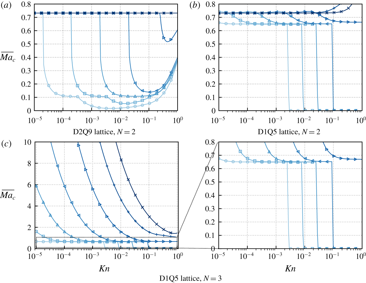
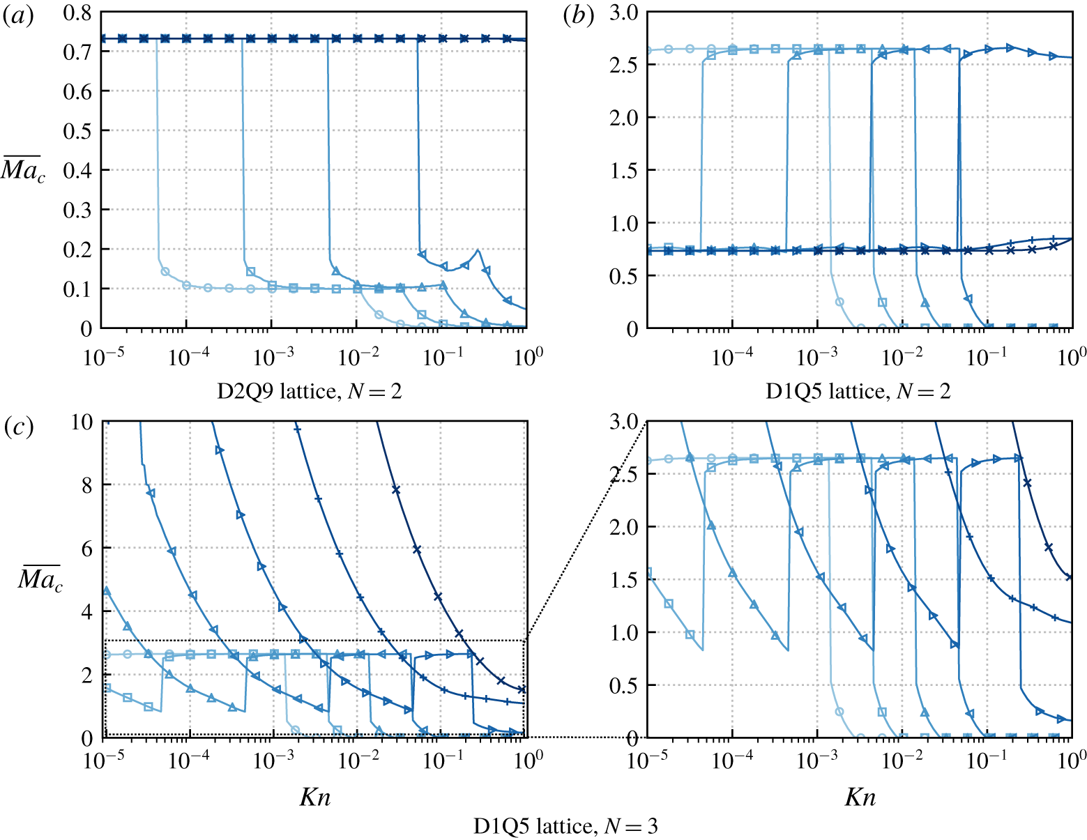
In fact, the proposed work on the DVBE can be seen as a limit framework encompassing all LBM. In §§ 3 and 4, we prove analytically that the critical Mach number of the D2Q9 is approximately 0.732 in the Gauss–Hermite case. It is exactly the limit observed empirically in the works of Hosseini et al. (Reference Hosseini, Coreixas, Darabiha and Thévenin2019) and Wissocq (Reference Wissocq2019) for large values of the reduced collision time. Proving further the generality of the proposed framework, multi-step LBM seem to show as well the same limiting critical Mach number (Wilde et al. Reference Wilde, Krämer, Küllmer, Foysi and Reith2019).

To the light of the following work, it is in fact possible to answer many questions often overlooked or swept under the carpet. For instance, which values of the reduced relaxation time still model a correct fluid for a given DVBE, possibly with a MRT model, or even the force terms? Which hydrodynamics regarding Navier–Stokes is resolved by the DVBE and thus by LBM in the convergent limit? The Knudsen–Shannon number is a useful conceptual tool to answer these questions. Now that the theoretical framework is settled, and the useful linkage with LBM performed, we can move to the analysis of actual lattices. Let us start with the D1Q3 lattice.

2.9 Remark – vocabulary used

We clarify further the important following notions used throughout the article:

1. (i) Equilibrium-rich DVBE: in the Gauss–Hermite framework, it defines a DVBE for which the truncation order $N$ is the highest possible whilst verifying $2N\leqslant Q$. In the moment-matching framework, it refers to a DVBE with fully matched Maxwell equilibrium moments. In both cases it defines the highest recovery of Maxwell moments with a given equilibrium construction procedure. With the Gauss–Hermite quadrature, slightly less moments are recovered due to the imposed orthogonality of the Hermite polynomials and the constraint of quadrature order.

2. (ii) Knudsen order: refers to the terms in the expansions in Knudsen number of $\unicode[STIX]{x1D714}_{\unicode[STIX]{x1D70F}}$, namely the $\unicode[STIX]{x1D714}_{\unicode[STIX]{x1D70F}_{j}}Kn^{j}$.

3. (iii) Standard lattices: refer to the lattices obtained by Gauss–Hermite quadrature, extensively studied in the literature.

4. (iv) Hydrodynamic waves: point out the two acoustic waves in the athermal case in one dimension, plus the shear wave(s) in multiple dimensions. These waves are identified via their developments in Knudsen number.

5. (v) Physics: refers to the dispersion and dissipation properties of the sets of equations under study, obtained through the eigenvalues.

3.1 The D1Q3 lattice closure on moments

In this discrete case, the macroscopic moments $\unicode[STIX]{x1D70C}$, $j$ and $\unicode[STIX]{x1D6F1}$ are naturally defined as

(3.1)$$\begin{eqnarray}\displaystyle & \displaystyle \unicode[STIX]{x1D70C}=m^{(0)}=\mathop{\sum }_{i=1}^{3}f_{i}, & \displaystyle\end{eqnarray}$$

(3.2)$$\begin{eqnarray}\displaystyle & \displaystyle j=\unicode[STIX]{x1D70C}u=m^{(1)}=\mathop{\sum }_{i=1}^{3}\unicode[STIX]{x1D709}_{i}\,f_{i}, & \displaystyle\end{eqnarray}$$

(3.3)$$\begin{eqnarray}\displaystyle & \displaystyle \unicode[STIX]{x1D6F1}=m^{(2)}=\mathop{\sum }_{i=1}^{3}\unicode[STIX]{x1D709}_{i}^{2}\,f_{i}. & \displaystyle\end{eqnarray}$$

We recall the notation $|\unicode[STIX]{x1D709}_{2}|=|\unicode[STIX]{x1D709}_{3}|=r$. So as to simplify future calculations, we further introduce a scaling parameter $\unicode[STIX]{x1D70E}$ defining the ratio between $r$ and the Newtonian sound speed $c=\sqrt{RT_{f}}$

(3.4)$$\begin{eqnarray}r=\unicode[STIX]{x1D70E}\sqrt{RT_{f}}=\unicode[STIX]{x1D70E}c.\end{eqnarray}$$

As discussed before, the finite-dimensional structure of the lattice enforces relations between higher- and lower-order moments, through a so-called lattice closure relation. In our D1Q3 case, it reads

(3.5)$$\begin{eqnarray}m^{(3)}=\mathop{\sum }_{i=1}^{3}\unicode[STIX]{x1D709}_{i}^{3}\,f_{i}=r^{3}f_{2}-r^{3}f_{3}=r^{2}(rf_{2}-rf_{3})=r^{2}m^{(1)}=r^{2}j=\unicode[STIX]{x1D70E}^{2}c^{2}j.\end{eqnarray}$$

3.2 Equivalent system and perturbative analysis

It is conspicuous that changing the descriptive variables of a system does not change the solutions $\unicode[STIX]{x1D714}_{\unicode[STIX]{x1D70F}}$. In our context, it allows us to work on the moment equations. Our interest is to catch visually the impact of the lattice closure and actually see the equilibrium moments. By taking the raw moments of the D1Q3 DVBE, we get

(3.6)$$\begin{eqnarray}\left.\begin{array}{@{}c@{}}\displaystyle \frac{\unicode[STIX]{x2202}\unicode[STIX]{x1D70C}}{\unicode[STIX]{x2202}t}+\frac{\unicode[STIX]{x2202}j}{\unicode[STIX]{x2202}x}=0,\\ \displaystyle \frac{\unicode[STIX]{x2202}j}{\unicode[STIX]{x2202}t}+\frac{\unicode[STIX]{x2202}\unicode[STIX]{x1D6F1}}{\unicode[STIX]{x2202}x}=0,\\ \displaystyle \frac{\unicode[STIX]{x2202}\unicode[STIX]{x1D6F1}}{\unicode[STIX]{x2202}t}+\underbrace{\unicode[STIX]{x1D70E}^{2}c^{2}\frac{\unicode[STIX]{x2202}j}{\unicode[STIX]{x2202}x}}_{closure\;relation}=-\frac{1}{\unicode[STIX]{x1D70F}}(\unicode[STIX]{x1D6F1}-\unicode[STIX]{x1D6F1}^{eq}),\end{array}\right\}\end{eqnarray}$$

where $\unicode[STIX]{x1D6F1}^{eq}=j^{2}/\unicode[STIX]{x1D70C}+\unicode[STIX]{x1D70C}c^{2}$ is the second-order equilibrium moment. We recognize a system whose two first equations express the conservation of mass and momentum. The last equation closes the system, showing the influence of collision. We can now perform our stability analysis over the set $(\unicode[STIX]{x1D70C},j,\unicode[STIX]{x1D6F1})$. The mean field is naturally denoted $(\overline{\unicode[STIX]{x1D70C}},\overline{j},\overline{\unicode[STIX]{x1D6F1}})$ and the mean Mach number of the flow $\overline{Ma}$ is defined as

(3.7)$$\begin{eqnarray}\overline{Ma}=\frac{\overline{j}}{\overline{\unicode[STIX]{x1D70C}}\sqrt{RT_{f}}}=\frac{\overline{j}}{\overline{\unicode[STIX]{x1D70C}}c}.\end{eqnarray}$$

This definition is arbitrary, and based on the Newtonian sound speed. The perturbative analysis presented in § 2 yields (2.26) under the explicit form

(3.8)$$\begin{eqnarray}\underbrace{\left(\begin{array}{@{}ccc@{}}\text{i}\unicode[STIX]{x1D714}_{\unicode[STIX]{x1D70F}} & -\text{i}\displaystyle \frac{Kn}{c} & 0\\ 0 & \text{i}\unicode[STIX]{x1D714}_{\unicode[STIX]{x1D70F}} & -\text{i}\displaystyle \frac{Kn}{c}\\ (\overline{Ma}^{2}-1)c^{2} & -(\text{i}Kn\unicode[STIX]{x1D70E}^{2}+2\overline{Ma})c & \text{i}\unicode[STIX]{x1D714}_{\unicode[STIX]{x1D70F}}+1\end{array}\right)}_{M_{D1Q3}}\left(\begin{array}{@{}c@{}}\hat{\unicode[STIX]{x1D70C}}\\ {\hat{j}}\\ \hat{\unicode[STIX]{x1D6F1}}\end{array}\right)=0,\end{eqnarray}$$

whose dispersion relation can be easily computed through

(3.9)$$\begin{eqnarray}\text{det}(M_{D1Q3})=0\;\Longleftrightarrow \;\text{i}\unicode[STIX]{x1D714}_{\unicode[STIX]{x1D70F}}^{3}+\unicode[STIX]{x1D714}_{\unicode[STIX]{x1D70F}}^{2}-Kn(\text{i}Kn\unicode[STIX]{x1D70E}^{2}+2\overline{Ma})\unicode[STIX]{x1D714}_{\unicode[STIX]{x1D70F}}+Kn^{2}(\overline{Ma}^{2}-1)=0.\end{eqnarray}$$

This equation, (3.9), can be solved analytically and has three complex solutions. But being of tremendous size, they are not given here. As announced, we rather provide the Taylor series expansion in Knudsen number (2.45) for each solution. The following forms are imposing but are insightful and will be commented on step by step. By looking at the first terms of the expansion, it is possible to identify clearly two acoustic waves ($\text{ac}+$), ($\text{ac}-$) and another one, which is named here the supplement ($s$). The acoustics ($\text{ac}\pm$) are exhibited through the terms $Kn(\overline{Ma}\pm 1)$, expressing a propagation at a reduced speed of 1 carried by the mean field $\overline{Ma}$. This behaviour recalls that of Euler, as shown in appendix B. For the downstream acoustic wave, we have

(3.10)$$\begin{eqnarray}\displaystyle \left.\begin{array}{@{}rcl@{}}\text{Re}(\unicode[STIX]{x1D714}_{\unicode[STIX]{x1D70F},ac+})\; & =\; & Kn(\overline{Ma}+1)\\ \; & \; & +\,Kn^{3} (\!\overline{Ma}^{6}-(2\unicode[STIX]{x1D70E}^{2}+15)\overline{Ma}^{4}-40\overline{Ma}^{3}+(\unicode[STIX]{x1D70E}^{4}+12\unicode[STIX]{x1D70E}^{2}-45)\overline{Ma}^{2}\\ \; & \; & +\,(16\unicode[STIX]{x1D70E}^{2}-24)\overline{Ma}-\unicode[STIX]{x1D70E}^{4}+6\unicode[STIX]{x1D70E}^{2}-5\!)\!/8\\ \; & \; & +\,O(Kn^{5}),\\ \text{Im}(\unicode[STIX]{x1D714}_{\unicode[STIX]{x1D70F},ac+})\; & =\; & Kn^{2}(-\overline{Ma}^{3}-3\overline{Ma}^{2}+(\unicode[STIX]{x1D70E}^{2}-3)\overline{Ma}+\unicode[STIX]{x1D70E}^{2}-1)/2\\ \; & \; & +\,Kn^{4} (\!\overline{Ma}^{9}-(3\unicode[STIX]{x1D70E}^{2}+12)\overline{Ma}^{7}+(3\unicode[STIX]{x1D70E}^{4}+21\unicode[STIX]{x1D70E}^{2}+126)\overline{Ma}^{5}+336\overline{Ma}^{4}\\ \; & \; & +\,(-\unicode[STIX]{x1D70E}^{6}-10\unicode[STIX]{x1D70E}^{4}-105\unicode[STIX]{x1D70E}^{2}+420)\overline{Ma}^{3}+(-168\unicode[STIX]{x1D70E}^{2}+288)\overline{Ma}^{2}\\ \; & \; & +\,(\unicode[STIX]{x1D70E}^{6}+15\unicode[STIX]{x1D70E}^{4}-105\unicode[STIX]{x1D70E}^{2}+105)\overline{Ma}+8\unicode[STIX]{x1D70E}^{4}-24\unicode[STIX]{x1D70E}^{2}+16\!)\!/16\\ \; & \; & +\,O(Kn^{6}),\end{array}\right\} & & \displaystyle \nonumber\\ \displaystyle & & \displaystyle\end{eqnarray}$$

for the upstream acoustic wave

(3.11)$$\begin{eqnarray}\displaystyle \left.\begin{array}{@{}rcl@{}}\text{Re}(\unicode[STIX]{x1D714}_{\unicode[STIX]{x1D70F},ac-})\; & =\; & Kn(\overline{Ma}-1)\\ \; & \; & +\,Kn^{3} (\!-\overline{Ma}^{6}+(2\unicode[STIX]{x1D70E}^{2}+15)\overline{Ma}^{4}-40\overline{Ma}^{3}+(-\unicode[STIX]{x1D70E}^{4}-12\unicode[STIX]{x1D70E}^{2}+45)\overline{Ma}^{2}\\ \; & \; & +\,(16\unicode[STIX]{x1D70E}^{2}-24)\overline{Ma}+\unicode[STIX]{x1D70E}^{4}-6\unicode[STIX]{x1D70E}^{2}+5\!)\!/8\\ \; & \; & +\,O(Kn^{5}),\\ \text{Im}(\unicode[STIX]{x1D714}_{\unicode[STIX]{x1D70F},ac-})\; & =\; & -Kn^{2}(\overline{Ma}-1)(\unicode[STIX]{x1D70E}^{2}-(\overline{Ma}-1)^{2})/2\\ \; & \; & +\,Kn^{4} (\!\overline{Ma}^{9}+(3\unicode[STIX]{x1D70E}^{2}+12)\overline{Ma}^{7}-(3\unicode[STIX]{x1D70E}^{4}+21\unicode[STIX]{x1D70E}^{2}+126)\overline{Ma}^{5}+336\overline{Ma}^{4}\\ \; & \; & +\,(\unicode[STIX]{x1D70E}^{6}+10\unicode[STIX]{x1D70E}^{4}+105\unicode[STIX]{x1D70E}^{2}-420)\overline{Ma}^{3}+(-168\unicode[STIX]{x1D70E}^{2}+288)\overline{Ma}^{2}\\ \; & \; & +\,(-\unicode[STIX]{x1D70E}^{6}-15\unicode[STIX]{x1D70E}^{4}+105\unicode[STIX]{x1D70E}^{2}-105)\overline{Ma}+8\unicode[STIX]{x1D70E}^{4}-24\unicode[STIX]{x1D70E}^{2}+16\!)\!/16\\ \; & \; & +\,O(Kn^{6}),\end{array}\right\} & & \displaystyle \nonumber\\ \displaystyle & & \displaystyle\end{eqnarray}$$

and for the supplement wave

(3.12)$$\begin{eqnarray}\displaystyle \left.\begin{array}{@{}rcl@{}}\text{Re}(\unicode[STIX]{x1D714}_{\unicode[STIX]{x1D70F},s})\; & =\; & -Kn(2\overline{Ma})\\ \; & \; & +\,Kn^{3}(10\overline{Ma}^{3}+(-4\unicode[STIX]{x1D70E}^{2}+6)\overline{Ma})\\ \; & \; & +\,O(Kn^{5}),\\ \text{Im}(\unicode[STIX]{x1D714}_{\unicode[STIX]{x1D70F},s})\; & =\; & 1\\ \; & \; & +\,Kn^{2}(3\overline{Ma}^{2}-\unicode[STIX]{x1D70E}^{2}+1)\\ \; & \; & +\,Kn^{4}(-42\overline{Ma}^{4}+(21\unicode[STIX]{x1D70E}^{2}-36)\overline{Ma}^{2}-\unicode[STIX]{x1D70E}^{4}+3\unicode[STIX]{x1D70E}^{2}-2)\\ \; & \; & +\,O(Kn^{6}).\end{array}\right\} & & \displaystyle\end{eqnarray}$$

3.3 Interpretation of the expansions

Let us now take a closer look at the solutions (3.10)–(3.12). We recall on the one hand that the real part provides the propagation properties of the waves, namely their phase and group speeds. On the other hand, the imaginary part describes the dissipation properties. With our convention for perturbations, a negative imaginary part leads to an exponentially growing linear instability. Note that the real part contains only odd powers in Knudsen number and the imaginary part only even ones. This can be physically explained. The sign of $Kn$ represents a direction of propagation but is just conventional. The dispersion $\text{Re}(\unicode[STIX]{x1D714}_{\unicode[STIX]{x1D70F}})$ of each wave must be an odd function because the phase speed switches sign with the direction considered. For its part, the dissipation $\text{Im}(\unicode[STIX]{x1D714}_{\unicode[STIX]{x1D70F}})$ is an even function, unchanged with respect to the direction considered.

As announced in § 2.8.1, the notion of Galilean invariance can be studied here at each Knudsen order. Here, for instance, the dependence of the dissipation in $Kn^{2}$ on the mean Mach number is a clear signature of Galilean variance. Terms in $\overline{Ma}^{3}$ intervene, as expected, because we are dealing with the $O(Ma^{3})$ error. One of the implications of this error is that the two acoustic waves do not propagate symmetrically. The scaling parameter $\unicode[STIX]{x1D70E}$, defining the lattice closure, appears in this error. Galilean invariance deviations can also be noted on dispersion with the terms in $Kn^{3}$ and beyond, by considering the phase and group speeds. Note that the terms in $Kn^{1}$ depend on the mean Mach number but do not exhibit Galilean variance, because what matters are the quantities $v_{g}-\overline{Ma}$ and $v_{\unicode[STIX]{x1D719}}-\overline{Ma}$.

3.4 Influence of the lattice closure through $\unicode[STIX]{x1D70E}$

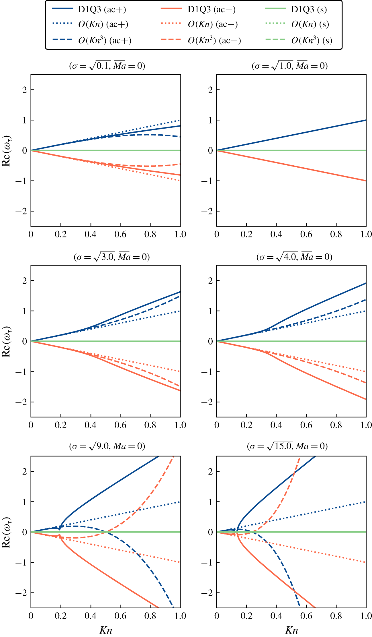
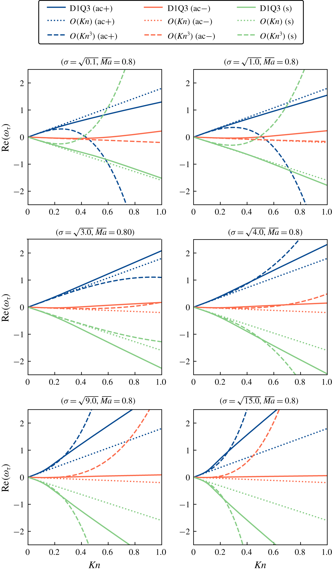
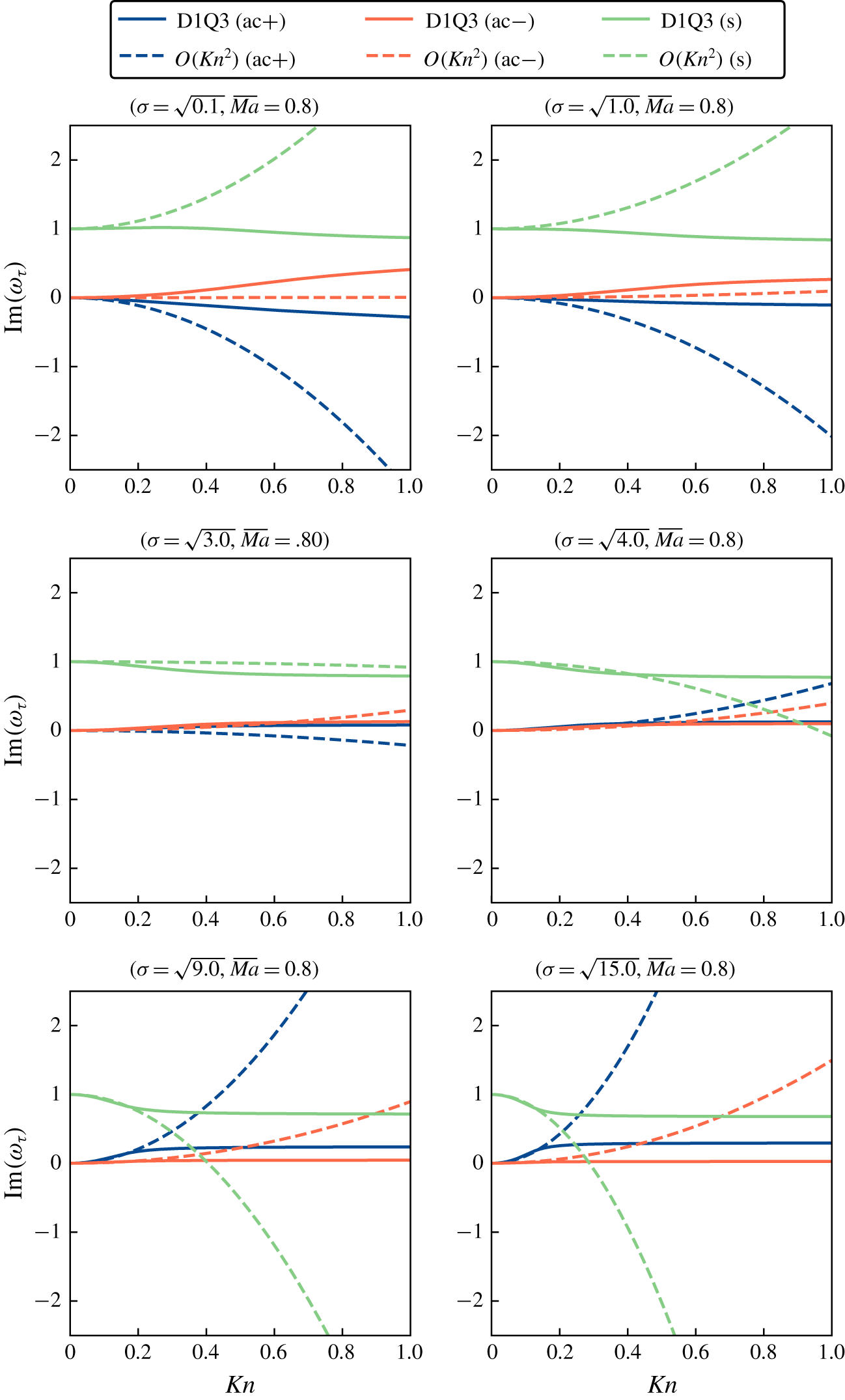
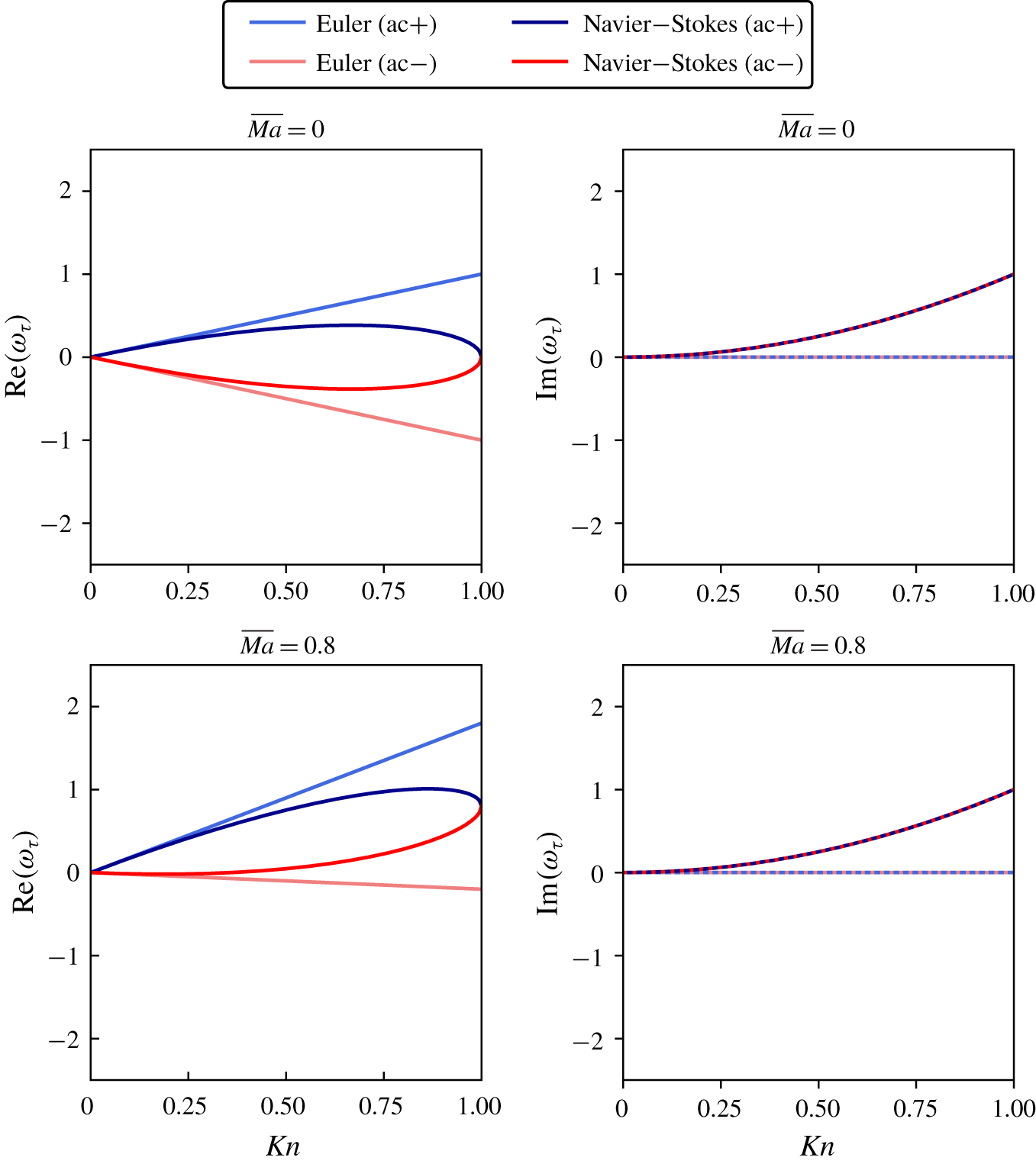
In figures 3, 4, 5 and 6 we plot the real and imaginary parts of the roots $\unicode[STIX]{x1D714}_{\unicode[STIX]{x1D70F}}$, successively for the mean Mach numbers 0 and 0.8. Some Taylor truncations are also plotted. The legend $O(Kn^{p})$ denotes a truncation of order $p$.

3.4.2 Dissipation and stability – $\text{Im}(\unicode[STIX]{x1D714}_{\unicode[STIX]{x1D70F}})$

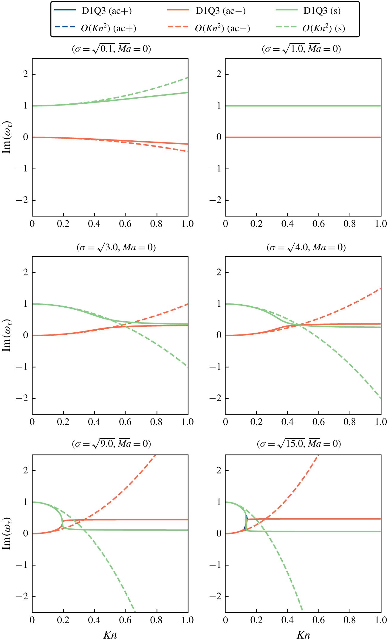
We now investigate some stability aspects of the D1Q3 lattice. The imaginary part of $\unicode[STIX]{x1D714}_{\unicode[STIX]{x1D70F}}$ is plotted in figures 4 and 6, respectively for the mean Mach numbers $\overline{Ma}=0$ and $\overline{Ma}=0.8$. As for the real part, the imaginary part does not fit well the Taylor development approximation for large Knudsen numbers, a situation which gets worse as $\unicode[STIX]{x1D70E}$ increases. This points out again that excessive values of $\unicode[STIX]{x1D70E}$ (typically ${\gtrsim}3$) cannot be easily studied analytically. We now restrict ourselves to reasonable, lesser values of $\unicode[STIX]{x1D70E}$ – what is the case of standard lattices – for which the second-order approximation fits reasonably well the analytical form. This happens by definition close to the origin, typically for $Kn\lesssim 0.5$. Within this framework, stability is approximately driven by the sign of the second-order truncation of the dissipation from (3.10)–(3.12)

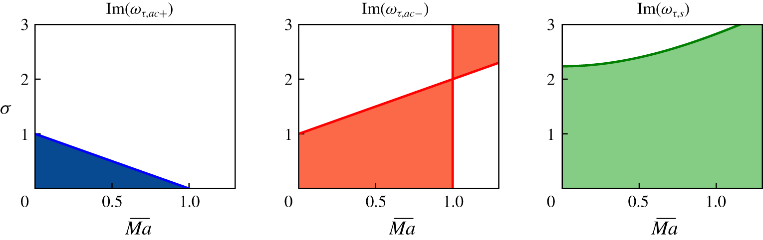
(3.13)$$\begin{eqnarray}\left.\begin{array}{@{}c@{}}\text{Im}(\unicode[STIX]{x1D714}_{\unicode[STIX]{x1D70F},ac+})\simeq Kn^{2}(\overline{Ma}+1)(\unicode[STIX]{x1D70E}^{2}-(\overline{Ma}+1)^{2})/2,\\ \text{Im}(\unicode[STIX]{x1D714}_{\unicode[STIX]{x1D70F},ac-})\simeq -Kn^{2}(\overline{Ma}-1)(\unicode[STIX]{x1D70E}^{2}-(\overline{Ma}-1)^{2})/2,\\ \text{Im}(\unicode[STIX]{x1D714}_{\unicode[STIX]{x1D70F},s})\simeq 1-Kn^{2}(\unicode[STIX]{x1D70E}^{2}-3\overline{Ma}^{2}-1).\end{array}\right\}\end{eqnarray}$$

The sign of these expressions is plotted in figure 2. The coloured regions exhibit the positive (stable) configurations. For the supplement wave, the most restrictive Knudsen number is considered ($Kn=0.5$ here). From these graphs it is clear that the wave driving the instability is always the downstream acoustic one. The critical Mach number $\overline{Ma}_{c}$ is therefore given by solving $(\unicode[STIX]{x1D70E}^{2}-(\overline{Ma}+1)^{2})=0$, which yields in our case

(3.14)$$\begin{eqnarray}\overline{Ma}_{c}=\unicode[STIX]{x1D70E}-1.\end{eqnarray}$$

Note that on the standard D1Q3 lattice, this critical Mach number evaluates to $\sqrt{3}-1\simeq 0.732$, a value encountered in practice in the LBM community (see Wilde et al. (Reference Wilde, Krämer, Küllmer, Foysi and Reith2019) and Hosseini et al. (Reference Hosseini, Coreixas, Darabiha and Thévenin2019) for example). Nonetheless, to the best of the authors’ knowledge, this specific value was never explained before. As will be seen in the next section, this critical Mach number is common to all lattices using a Gauss–Hermite quadrature with $N=2$. They suffer from an intrinsically rough lattice closure and/or quadrature order, thus a Galilean variance in $Kn^{2}$. It means that, without any modification to the DVBE, LBM schemes with $N=2$ cannot cope with transonic or supersonic flows. In the next paragraph, we see, however, that it is possible to amend the DVBE by adding forcing terms, so as to establish Galilean invariance in $Kn^{2}$ even when $N=2$.

Figure 2.

Sign of the truncated imaginary parts (up to the second order in $Kn$) for each of the waves, as a function of $\unicode[STIX]{x1D70E}$ and $\overline{Ma}$. The coloured regions are the positive regions, while the regions left blank are the negative regions.

Figure 3.

Real part of the complex angular velocities $\unicode[STIX]{x1D714}_{\unicode[STIX]{x1D70F}}$, solutions of the dispersion equation, for $\overline{Ma}=0$.

Figure 4.

Imaginary part of the complex angular velocities $\unicode[STIX]{x1D714}_{\unicode[STIX]{x1D70F}}$, solutions of the dispersion equation, for $\overline{Ma}=0$.

Figure 5.

Real part of the complex angular velocities $\unicode[STIX]{x1D714}_{\unicode[STIX]{x1D70F}}$, solutions of the dispersion equation, for $\overline{Ma}=0.8$.

Figure 6.

Imaginary part of the complex angular velocities $\unicode[STIX]{x1D714}_{\unicode[STIX]{x1D70F}}$, solutions of the dispersion equation, for $\overline{Ma}=0.8$.

3.5 Corrective terms to tailor the Knudsen orders

There is no reason for any DVBE to be Galilean invariant at all Knudsen orders – this point is notably addressed thoroughly in § 5. As explained in the previous paragraph, most simple-speed lattices, used in many solvers because they are well adapted to stream-and-collide algorithms, suffer from this problem from the second Knudsen order ($Kn^{2}$). So as to address this issue, it is possible to modify the DVBE by introducing a force term $\unicode[STIX]{x1D713}_{i}$ (also called corrective term) as follows:

(3.15)$$\begin{eqnarray}\frac{\unicode[STIX]{x2202}f_{i}}{\unicode[STIX]{x2202}t}+\unicode[STIX]{x1D709}_{i_{\unicode[STIX]{x1D6FC}}}\frac{\unicode[STIX]{x2202}f_{i}}{\unicode[STIX]{x2202}\unicode[STIX]{x1D6FC}}=-\frac{1}{\unicode[STIX]{x1D70F}}(\,f_{i}-f_{i}^{eq})+\unicode[STIX]{x1D713}_{i}.\end{eqnarray}$$

This approach is well known in the LBM community (Prasianakis & Karlin Reference Prasianakis and Karlin2007; Feng et al. Reference Feng, Boivin, Jacob and Sagaut2019). Its purpose is to suppress the so-called $O(Ma^{3})$ error in the momentum equation obtained through a Chapman–Enskog procedure. On standard lattices in one dimension and for thermal cases, this term can be written under the form

(3.16)$$\begin{eqnarray}\unicode[STIX]{x1D713}_{i}\propto {\mathcal{H}}_{i}^{(2)}\frac{\unicode[STIX]{x2202}}{\unicode[STIX]{x2202}x}[\unicode[STIX]{x1D70C}u((1-\unicode[STIX]{x1D703})c_{0}^{2}-u^{2})],\end{eqnarray}$$

where $\unicode[STIX]{x1D703}$ is a dimensionless temperature and $c_{0}$ a certain speed, both adapted to Gauss–Hermite thermal cases. The term is traditionally constructed so that its zeroth and first moments are null, while the second-order moment yields the following correction on the second-order moment equation:

(3.17)$$\begin{eqnarray}\mathop{\sum }_{i=1}^{3}\unicode[STIX]{x1D709}_{i}^{2}\unicode[STIX]{x1D713}_{i}=\frac{\unicode[STIX]{x2202}}{\unicode[STIX]{x2202}x}[\unicode[STIX]{x1D70C}u((1-\unicode[STIX]{x1D703})c_{0}^{2}-u^{2})].\end{eqnarray}$$

We still consider the D1Q3 lattice. The term $\unicode[STIX]{x1D713}_{i}$ has to be adapted to the present framework with a general lattice closure and the athermal hypothesis. We must notably adapt the Hermite polynomials to a more general expression taking into account $\unicode[STIX]{x1D70E}$. On the other hand, even in the athermal framework, we keep the dimensionless temperature $\unicode[STIX]{x1D703}$ as an extra degree of freedom, an a priori function of $\unicode[STIX]{x1D70E}$. This will notably help us recover interesting Galilean invariant properties. The final form of our corrective term is thus

(3.18)$$\begin{eqnarray}\unicode[STIX]{x1D713}_{i}(\unicode[STIX]{x1D70E})=w_{i}\frac{3\unicode[STIX]{x1D709}_{i}^{2}-\unicode[STIX]{x1D70E}^{2}c^{2}}{2\unicode[STIX]{x1D70E}^{4}c^{4}}\frac{\unicode[STIX]{x2202}}{\unicode[STIX]{x2202}x}[\unicode[STIX]{x1D70C}u((1-\unicode[STIX]{x1D703}(\unicode[STIX]{x1D70E}))c^{2}-u^{2})],\end{eqnarray}$$

where $w_{1}=2/3$, $w_{2}=w_{3}=1/6$. The system (3.6) now reads

(3.19)$$\begin{eqnarray}\left.\begin{array}{@{}c@{}}\displaystyle \frac{\unicode[STIX]{x2202}\unicode[STIX]{x1D70C}}{\unicode[STIX]{x2202}t}+\frac{\unicode[STIX]{x2202}j}{\unicode[STIX]{x2202}x}=0,\\ \displaystyle \frac{\unicode[STIX]{x2202}j}{\unicode[STIX]{x2202}t}+\frac{\unicode[STIX]{x2202}\unicode[STIX]{x1D6F1}}{\unicode[STIX]{x2202}x}=0,\\ \displaystyle \frac{\unicode[STIX]{x2202}\unicode[STIX]{x1D6F1}}{\unicode[STIX]{x2202}t}+\unicode[STIX]{x1D70E}^{2}c^{2}\frac{\unicode[STIX]{x2202}j}{\unicode[STIX]{x2202}x}=-\frac{1}{\unicode[STIX]{x1D70F}}(\unicode[STIX]{x1D6F1}-\unicode[STIX]{x1D6F1}^{eq})+\frac{\unicode[STIX]{x2202}}{\unicode[STIX]{x2202}x}[\unicode[STIX]{x1D70C}u((1-\unicode[STIX]{x1D703}(\unicode[STIX]{x1D70E}))c^{2}-u^{2})].\end{array}\right\}\end{eqnarray}$$

It is possible to perform a perturbative analysis as previously. As before, we provide the second-order Taylor development of the imaginary parts

(3.20)$$\begin{eqnarray}\left.\begin{array}{@{}c@{}}\displaystyle \text{Im}(\unicode[STIX]{x1D714}_{\unicode[STIX]{x1D70F},ac+})=Kn^{2}(1+{\textstyle \frac{1}{2}}(\unicode[STIX]{x1D703}(\unicode[STIX]{x1D70E})-4+\unicode[STIX]{x1D70E}^{2})(\overline{Ma}+1))+O(Kn^{4}),\\ \displaystyle \text{Im}(\unicode[STIX]{x1D714}_{\unicode[STIX]{x1D70F},ac-})=Kn^{2}(1-{\textstyle \frac{1}{2}}(\unicode[STIX]{x1D703}(\unicode[STIX]{x1D70E})-4+\unicode[STIX]{x1D70E}^{2})(\overline{Ma}-1))+O(Kn^{4}),\\ \displaystyle \text{Im}(\unicode[STIX]{x1D714}_{\unicode[STIX]{x1D70F},s})=1-Kn^{2}(\unicode[STIX]{x1D703}(\unicode[STIX]{x1D70E})-2+\unicode[STIX]{x1D70E}^{2})+O(Kn^{4}).\end{array}\right\}\end{eqnarray}$$

The force term changed (3.13) into (3.20). Interesting remarks can now be made. The first is that choosing

(3.21)$$\begin{eqnarray}\unicode[STIX]{x1D703}(\unicode[STIX]{x1D70E})=4-\unicode[STIX]{x1D70E}^{2},\end{eqnarray}$$

recovers Galilean invariance in $Kn^{2}$. The second is that keeping the extra parameter $\unicode[STIX]{x1D703}$, even in the athermal case, is necessary to retrieve this invariance. A thermal analysis would not allow for this supplementary degree of freedom, since $\unicode[STIX]{x1D703}$ would be a new independent parameter. Note also that with $\unicode[STIX]{x1D70E}=\sqrt{3}$ and $\unicode[STIX]{x1D703}=1$, the term proportional to $\unicode[STIX]{x1D70C}u$ in (3.18) disappears. From there it is thus impossible to ascertain that the Galilean invariance is indeed retrieved in practical thermal cases, which will be investigated in future work. We also remark that the term obtained at the second order for the acoustic waves fits that of the Navier–Stokes dissipation, which is exactly $\text{Im}(\unicode[STIX]{x1D714}_{\unicode[STIX]{x1D70F},ac\pm })_{NS}=iKn^{2}$ (see appendix B). The non-null higher-order dissipative terms of the corrected D1Q3 lattice are thus direct deviations from Navier–Stokes. So if one wants to recover this behaviour, these higher-order terms should all be set to zero. To achieve it, we can push the reasoning to the next level and propose additional corrective terms. For that, let us for instance take a look at the fourth-order coefficient of the downstream acoustic wave ($ac+$) taking into account the above correction term with (3.21). We find

(3.22)$$\begin{eqnarray}\unicode[STIX]{x1D714}_{\unicode[STIX]{x1D70F}_{4},ac+}=Kn^{4}(-9\overline{Ma}^{2}-3\overline{Ma}+1).\end{eqnarray}$$

This term is not zero, nor Galilean invariant. And since it shows mean Mach numbers to the zeroth, first and second powers at a fourth order in Knudsen number, inspired by the previous force term $\unicode[STIX]{x1D713}_{i}$, it is possible to imagine an additional correction $\unicode[STIX]{x1D719}_{i}$ of the form

(3.23)$$\begin{eqnarray}\unicode[STIX]{x1D719}_{i}=w_{i}\frac{3\unicode[STIX]{x1D709}_{i}^{2}-\unicode[STIX]{x1D70E}^{2}c^{2}}{2\unicode[STIX]{x1D70E}^{4}c^{4}}(c\unicode[STIX]{x1D70F})^{2}\frac{\unicode[STIX]{x2202}^{3}}{\unicode[STIX]{x2202}x^{3}}\left[\unicode[STIX]{x1D706}_{0}\unicode[STIX]{x1D70C}c^{3}+\unicode[STIX]{x1D706}_{1}\,jc^{2}+\unicode[STIX]{x1D706}_{2}\frac{j^{2}}{\unicode[STIX]{x1D70C}}c\right].\end{eqnarray}$$

The third-order derivative after a linearization process leads to a term $\propto Kn^{3}$ in the perturbation matrix, and thus does not change lower orders which were already correct. The cascade which appears with the terms $-\text{i}Kn/c$ in all perturbation matrices above the diagonal will increase by one the affected Knudsen order, here in $Kn^{4}$. The linear combination of $\unicode[STIX]{x1D70C}$, $j$ and $j^{2}/\unicode[STIX]{x1D70C}$ leads to a linear combination of terms in $\overline{Ma}^{0}=1$, $\overline{Ma}^{1}$ and $\overline{Ma}^{2}$ to try and enforce Galilean invariance and nullify the term completely. In our case, the coefficient from (3.22) now reads

(3.24)$$\begin{eqnarray}\unicode[STIX]{x1D714}_{\unicode[STIX]{x1D70F}_{4},ac+}=Kn^{4}(\overline{Ma}^{2}(\unicode[STIX]{x1D706}_{2}+18)+\overline{Ma}(2\unicode[STIX]{x1D706}_{2}+\unicode[STIX]{x1D706}_{1}+6)+\unicode[STIX]{x1D706}_{1}+\unicode[STIX]{x1D706}_{0}-2).\end{eqnarray}$$

Choosing $\unicode[STIX]{x1D706}_{2}=-18$, $\unicode[STIX]{x1D706}_{1}=30$ and $\unicode[STIX]{x1D706}_{0}=-28$ nullifies this coefficient, as expected for a Navier–Stokes behaviour. However, the upstream acoustic wave ($ac-$) is not corrected simultaneously. A general method must be further adapted and investigated, but would stand outside of the scope of this article. The various levels of the super-Burnett equations could give hints towards forms of corrections, leading to an independence from the mean flow for the even Knudsen orders (see § 5). Here, the purpose was to underline the levers at the disposal of one willing to design force terms.

Instead of adding corrective terms to the DVBE, it is possible to enrich naturally the physics and retrieve Galilean invariance at certain Knudsen orders. For instance, we now see with the D1Q4 lattice that a correct dissipation of the acoustic waves is obtained as soon as the third-order Maxwell moment is recovered. More generally, an increase in number of discrete velocities and recovered Maxwell moments leads to more and more converged physics, as explained thoroughly in § 5.

4.1 The question of larger lattices

The analytical study of a lattice with $V$ discrete velocities requires the extraction of $V$ complex roots from the dispersion relation. Since we wish to work completely analytically, these roots have to be resolved formally in the general case. Unfortunately, this is mathematically impossible: the roots of any (even complex) polynomial of order ${\geqslant}5$ cannot be expressed through radicals in the general case, as proved a long time ago by Abel (Reference Abel1824). In practice, this means that extracting the solutions for the D1Q5 or D2Q9 lattices, for instance, is not feasible. Even though this drawback strongly restricts the frame of study of the proposed methodology, the D1Q4 is still feasible and we will see that it brings valuable information on the behaviour of the DVBE for larger lattices.

4.2 MRT models

As we have seen in the previous section, the simple BGK operator has fundamental limitations in terms of stability. In addition to this intrinsic drawback, LBM schemes must cope with additional instabilities arising from the space–time discretization. One way of reducing these numerical instabilities is the introduction of a MRT modelling (Lallemand & Luo Reference Lallemand and Luo2000). The principle of MRT models is to relax given moments at different frequencies. This formalism is more general than the DVBE presented in (2.14). More importantly, note that the Chapman–Enskog expansion and its implications presented in § 5 should not apply, because the underlying logic of identifying terms related to a unique $\unicode[STIX]{x1D70F}$ does not hold anymore. The relative importance of higher-order contributions must be investigated. And fortunately, the perturbative methodology still holds and provides expansions in Knudsen number without use of the Chapman–Enskog expansion. As originally proposed by d’Humières (Reference d’Humières1992), all MRT models can be written in the form (here in one dimension)

(4.1)$$\begin{eqnarray}\frac{\unicode[STIX]{x2202}\boldsymbol{{\mathcal{F}}}}{\unicode[STIX]{x2202}t}+\frac{\unicode[STIX]{x2202}(\unicode[STIX]{x1D743}\boldsymbol{{\mathcal{F}}})}{\unicode[STIX]{x2202}x}=\unicode[STIX]{x1D648}^{-1}\pmb{\unicode[STIX]{x1D6EC}}\unicode[STIX]{x1D648}(\boldsymbol{{\mathcal{F}}}-\boldsymbol{{\mathcal{F}}}^{\boldsymbol{e}\boldsymbol{q}}),\end{eqnarray}$$

where $\unicode[STIX]{x1D743}\boldsymbol{{\mathcal{F}}}$ denotes simply the vector of $(\unicode[STIX]{x1D709}_{i}\,f_{i})_{i\in \unicode[STIX]{x27E6}1,V\unicode[STIX]{x27E7}}$; $\unicode[STIX]{x1D648}$ is a general passage matrix providing the basis for collision. The diagonal matrix $\pmb{\unicode[STIX]{x1D6EC}}$ sets an independent collision frequency for each moment. Many choices can be made for the collision basis. It could be a priori completely arbitrary, providing a wide range of fluidic properties. Yet, in general, the first moments are collision invariants and the first corresponding terms in the diagonal of $\pmb{\unicode[STIX]{x1D6EC}}$ are useless – and thus set to zero.

MRT models are used in a wide range of applications. One of their most famous forms was developed in the early work of d’Humieres (Reference d’Humieres2002), in the case of the D3Q15 and D3Q19 lattices. MRT models also provided LBM a better management of boundary conditions (Ginzbourg & Adler Reference Ginzbourg and Adler1994), improved thermal properties (McNamara, Garcia & Alder Reference McNamara, Garcia and Alder1995) and the ability to retrieve visco-elastic behaviour (Giraud, d’Humières & Lallemand Reference Giraud, d’Humières and Lallemand1997). On the other hand, although stabilizing many simulations, MRT models might result in less physical interfacial dynamics of liquid ligaments in multiphase flows, by changing the distribution of spurious currents at the interface (Chiappini et al. Reference Chiappini, Sbragaglia, Xue and Falcucci2019). Note that some regularization procedures can be written under the form of MRT (Latt & Chopard Reference Latt and Chopard2006). Later, Geier et al. (Reference Geier, Greiner and Korvink2006) pioneered a cascaded model, which is based on a central-moment collision. In that case, the matrix $\unicode[STIX]{x1D648}$ depends upon the local flow, through a shift of the lattice velocities by the local flow speed. This modelling claimed to restore Galilean invariance, which is equivalent to suppress the $O(Ma^{3})$ error on simple-speed lattices. In that context, using a D1Q4 lattice, we are to catch the influence on hydrodynamics, stability and the related Galilean invariance errors arising from MRT and cascaded models. Do they improve the intrinsic stability of the equations, or are the observed improvements solely numerical?

4.3 The generalized MRT-D1Q4 lattice

The purpose of this paragraph is to set up a generalized MRT-D1Q4 model, with a unified formalism which allows us to identify simultaneously the influence of:

1. (i) the enrichment equilibrium;

2. (ii) the addition of discrete velocities;

3. (iii) the introduction of an additional relaxation parameter through a MRT model;

4. (iv) and the choice of the collision basis when moving to central moments.

This formalism encompasses BGK and some basic MRT models. The prescribed velocities of the lattice are shown in figure 7. We set $\unicode[STIX]{x1D709}_{1}=r$, $\unicode[STIX]{x1D709}_{2}=2r$, $\unicode[STIX]{x1D709}_{3}=-r$ and $\unicode[STIX]{x1D709}_{4}=-2r$, where $r=\unicode[STIX]{x1D70E}c$, as in the previous section. With the D1Q4 lattice, it is possible to represent an additional independent moment $Q=m^{(3)}$, because the lattice closure is pushed one moment equation farther. In our case, this closure relation reads

(4.2)$$\begin{eqnarray}m^{(4)}=5\unicode[STIX]{x1D70E}^{2}c^{2}\unicode[STIX]{x1D6F1}-4\unicode[STIX]{x1D70E}^{4}c^{4}\unicode[STIX]{x1D70C}.\end{eqnarray}$$

We note $\boldsymbol{{\mathcal{M}}}=(m^{(n)})_{n\in \unicode[STIX]{x27E6}1,V\unicode[STIX]{x27E7}}$ and $\boldsymbol{{\mathcal{M}}}_{\boldsymbol{c}}=(m_{c}^{(n)})_{n\in \unicode[STIX]{x27E6}1,V\unicode[STIX]{x27E7}}$ for which $m_{c}^{(n)}$ refers to the central moments defined by

(4.3)$$\begin{eqnarray}m_{c}^{(n)}=\mathop{\sum }_{i=1}^{V}(\unicode[STIX]{x1D709}_{i}-u)^{n}f_{i}=\mathop{\sum }_{i=1}^{V}\left(\unicode[STIX]{x1D709}_{i}-\frac{j}{\unicode[STIX]{x1D70C}}\right)^{n}f_{i},\end{eqnarray}$$

in the one-dimensional case. We also introduce the two passage matrices $\unicode[STIX]{x1D648}_{\boldsymbol{r}}$ and $\unicode[STIX]{x1D648}_{\boldsymbol{c}}$, respectively yielding the raw and central moments from the discrete distributions

(4.4a,b)$$\begin{eqnarray}\displaystyle \boldsymbol{{\mathcal{M}}}=\unicode[STIX]{x1D648}_{\boldsymbol{r}}\boldsymbol{{\mathcal{F}}}\quad \text{and}\quad \boldsymbol{{\mathcal{M}}}_{\boldsymbol{c}}=\unicode[STIX]{x1D648}_{\boldsymbol{c}}\boldsymbol{{\mathcal{F}}}. & & \displaystyle\end{eqnarray}$$

Explicitly, those matrices read in our D1Q4 case

(4.5)$$\begin{eqnarray}\unicode[STIX]{x1D648}_{\boldsymbol{r}}=\left(\begin{array}{@{}cccc@{}}1 & 1 & 1 & 1\\ r & 2r & -r & -2r\\ r^{2} & 4r^{2} & r^{2} & 4r^{2}\\ r^{3} & 8r^{3} & -r^{3} & -8r^{3}\end{array}\right),\end{eqnarray}$$

and

(4.6)$$\begin{eqnarray}\unicode[STIX]{x1D648}_{\boldsymbol{c}}=\left(\begin{array}{@{}cccc@{}}1 & 1 & 1 & 1\\ r-u & 2r-u & -r-u & -2r-u\\ (r-u)^{2} & (2r-u)^{2} & (-r-u)^{2} & (-2r-u)^{2}\\ (r-u)^{3} & (2r-u)^{3} & (-r-u)^{3} & (-2r-u)^{3}\end{array}\right).\end{eqnarray}$$

Figure 7.

Sketch of the D1Q4 lattice.

For the sake of compactness and generality, we introduce a switch parameter $\unicode[STIX]{x1D6FF}$ which defines whether we compute raw ($\unicode[STIX]{x1D6FF}=0$) or central moments ($\unicode[STIX]{x1D6FF}=1$). With it, we define a general passage matrix $\unicode[STIX]{x1D648}_{\unicode[STIX]{x1D739}}$ encompassing the two definitions

(4.7)$$\begin{eqnarray}\unicode[STIX]{x1D648}_{\unicode[STIX]{x1D739}}=(1-\unicode[STIX]{x1D6FF})\unicode[STIX]{x1D648}_{\boldsymbol{r}}+\unicode[STIX]{x1D6FF}\unicode[STIX]{x1D648}_{\boldsymbol{c}},\end{eqnarray}$$

and the associated general moments

(4.8)$$\begin{eqnarray}\boldsymbol{{\mathcal{M}}}_{\unicode[STIX]{x1D739}}=\unicode[STIX]{x1D648}_{\unicode[STIX]{x1D739}}\boldsymbol{{\mathcal{F}}}=(1-\unicode[STIX]{x1D6FF})\boldsymbol{{\mathcal{M}}}+\unicode[STIX]{x1D6FF}\boldsymbol{{\mathcal{M}}}_{\boldsymbol{c}}.\end{eqnarray}$$

Equation (4.1) reads in our particular case

(4.9)$$\begin{eqnarray}\frac{\unicode[STIX]{x2202}\boldsymbol{{\mathcal{F}}}}{\unicode[STIX]{x2202}t}+\frac{\unicode[STIX]{x2202}(\unicode[STIX]{x1D743}\boldsymbol{{\mathcal{F}}})}{\unicode[STIX]{x2202}x}=\unicode[STIX]{x1D648}_{\unicode[STIX]{x1D739}}^{-1}\pmb{\unicode[STIX]{x1D6EC}}\unicode[STIX]{x1D648}_{\unicode[STIX]{x1D739}}(\boldsymbol{{\mathcal{F}}}-\boldsymbol{{\mathcal{F}}}^{\boldsymbol{e}\boldsymbol{q}}),\end{eqnarray}$$

for which we set second relaxation time $\unicode[STIX]{x1D70F}_{N}$ associated with the MRT model in $\unicode[STIX]{x1D6EC}$

(4.10)$$\begin{eqnarray}\pmb{\unicode[STIX]{x1D6EC}}=\left(\begin{array}{@{}cccc@{}}0 & & & \\ & 0 & & \\ & & -\displaystyle \frac{1}{\unicode[STIX]{x1D70F}} & \\ & & & -\displaystyle \frac{1}{\unicode[STIX]{x1D70F}_{N}}\end{array}\right).\end{eqnarray}$$

Since we have introduced a new dimensional parameter $\unicode[STIX]{x1D70F}_{N}$ into the equations, another dimensionless parameter must be set up and will naturally appear in the solutions. To this regard, we denote the ratio

(4.11)$$\begin{eqnarray}\frac{\unicode[STIX]{x1D70F}}{\unicode[STIX]{x1D70F}_{N}}=Pr,\end{eqnarray}$$

as a certain Prandtl number, since it models the ratio between the relaxation times of the momentum and the energy fluxes. However, since our athermal approximation does not model an energy-conserving fluid, this definition must not be considered absolute. Eventually, the last ingredient of this modelling consists in tailoring the third-order (raw) equilibrium moment, through the introduction of a second switch parameter $\unicode[STIX]{x1D6FE}$ to set the richness of the equilibrium, so that

(4.12)$$\begin{eqnarray}Q_{\unicode[STIX]{x1D6FE}}^{eq}=\unicode[STIX]{x1D6FE}(\unicode[STIX]{x1D70C}u^{3}+3\unicode[STIX]{x1D70C}uc^{2})=\unicode[STIX]{x1D6FE}\left(\frac{j^{3}}{\unicode[STIX]{x1D70C}^{2}}+3jc^{2}\right).\end{eqnarray}$$

If $\unicode[STIX]{x1D6FE}=0$, the equilibrium is not enriched compared to the previous D1Q3 lattice. On the other hand, if $\unicode[STIX]{x1D6FE}=1$, all possible Maxwell moments are matched.

4.4 Perturbative analysis of the generalized MRT-D1Q4 model

A perturbative analysis of (4.9) is now performed. By taking the raw moments of the system of equations, which is equivalent to multiplying (4.9) by $\unicode[STIX]{x1D648}_{\boldsymbol{r}}$, we get

(4.13)$$\begin{eqnarray}\left(\begin{array}{@{}cccc@{}}\text{i}\unicode[STIX]{x1D714}_{\unicode[STIX]{x1D70F}} & -\text{i}\displaystyle \frac{Kn}{c} & 0 & 0\\ 0 & \text{i}\unicode[STIX]{x1D714}_{\unicode[STIX]{x1D70F}} & -\text{i}\displaystyle \frac{Kn}{c} & 0\\ (\overline{Ma}^{2}-1)c^{2} & -2\overline{Ma}c & \text{i}\unicode[STIX]{x1D714}_{\unicode[STIX]{x1D70F}}+1 & -\text{i}\displaystyle \frac{Kn}{c}\\ m_{41} & m_{42} & (-5\text{i}\unicode[STIX]{x1D70E}^{2}Kn+3\unicode[STIX]{x1D6FF}\overline{Ma}(1-Pr))c & \text{i}\unicode[STIX]{x1D714}_{\unicode[STIX]{x1D70F}}+Pr\end{array}\right)\left(\begin{array}{@{}c@{}}\hat{\unicode[STIX]{x1D70C}}\\ {\hat{j}}\\ \hat{\unicode[STIX]{x1D6F1}}\\ \hat{Q}\end{array}\right)=0,\end{eqnarray}$$

where $m_{41}=(4\text{i}\unicode[STIX]{x1D70E}^{4}Kn+2\unicode[STIX]{x1D6FE}Pr\overline{Ma}^{3}+3\unicode[STIX]{x1D6FF}\overline{Ma}(\overline{Ma}^{2}-1)(1-Pr))c^{3}$ and $m_{42}=(-3\unicode[STIX]{x1D6FE}Pr(\overline{Ma}^{2}+1)+6\unicode[STIX]{x1D6FF}\overline{Ma}^{2}(Pr-1))c^{2}$. Contrary to the D1Q3 lattice, we have this time four solutions. We recognize again two acoustic waves ($\text{ac}+$) and ($\text{ac}-$) through the first dispersion order of the form $Kn(\overline{Ma}\pm 1)$. The two supplementary waves are noted ($\text{s}_{1}$) and ($\text{s}_{2}$). We provide the Taylor developments, first of the downstream acoustic wave

(4.14)$$\begin{eqnarray}\displaystyle \left.\begin{array}{@{}rcl@{}}\text{Re}(\unicode[STIX]{x1D714}_{\unicode[STIX]{x1D70F},ac+})\; & =\; & Kn(\overline{Ma}+1)\\ \; & \; & +\,Kn^{3}\displaystyle \frac{f(\overline{Ma},Pr,\unicode[STIX]{x1D6FF},\unicode[STIX]{x1D6FE},\unicode[STIX]{x1D70E})}{8Pr}\\ \; & \; & +\,O(Kn^{5}),\\ \text{Im}(\unicode[STIX]{x1D714}_{\unicode[STIX]{x1D70F},ac+})\; & =\; & Kn^{2}[1+(\unicode[STIX]{x1D6FE}-1)(\overline{Ma}^{3}+3\overline{Ma}^{2}+3\overline{Ma}+3)]\\ \; & \; & +\,Kn^{4}\displaystyle \frac{f(\overline{Ma},Pr,\unicode[STIX]{x1D6FF},\unicode[STIX]{x1D6FE},\unicode[STIX]{x1D70E})}{16Pr^{2}}\\ \; & \; & +\,O(Kn^{6}),\end{array}\right\} & & \displaystyle\end{eqnarray}$$

then of the upstream one

(4.15)$$\begin{eqnarray}\displaystyle \left.\begin{array}{@{}rcl@{}}\text{Re}(\unicode[STIX]{x1D714}_{\unicode[STIX]{x1D70F},ac-})\; & =\; & Kn(\overline{Ma}-1)\\ \; & \; & +\,Kn^{3}\displaystyle \frac{f(\overline{Ma},Pr,\unicode[STIX]{x1D6FF},\unicode[STIX]{x1D6FE},\unicode[STIX]{x1D70E})}{8Pr}\\ \; & \; & +\,O(Kn^{5}),\\ \text{Im}(\unicode[STIX]{x1D714}_{\unicode[STIX]{x1D70F},ac-})\; & =\; & Kn^{2}[1-(\unicode[STIX]{x1D6FE}-1)(\overline{Ma}^{3}-3\overline{Ma}^{2}+3\overline{Ma}-3)]\\ \; & \; & +\,Kn^{4}\displaystyle \frac{f(\overline{Ma},Pr,\unicode[STIX]{x1D6FF},\unicode[STIX]{x1D6FE},\unicode[STIX]{x1D70E})}{16Pr^{2}}\\ \; & \; & +\,O(Kn^{6}).\end{array}\right\} & & \displaystyle\end{eqnarray}$$

The first supplementary wave reads

(4.16)$$\begin{eqnarray}\displaystyle \left.\begin{array}{@{}rcl@{}}\text{Re}(\unicode[STIX]{x1D714}_{\unicode[STIX]{x1D70F},s_{1}})\; & =\; & Kn[\overline{Ma}(3\unicode[STIX]{x1D6FF}-2)]\\ \; & \; & +\,Kn^{3}\displaystyle \frac{f(\overline{Ma},Pr,\unicode[STIX]{x1D6FF},\unicode[STIX]{x1D6FE},\unicode[STIX]{x1D70E})}{(Pr-1)^{2}}\\ \; & \; & +\,O(Kn^{5}),\\ \text{Im}(\unicode[STIX]{x1D714}_{\unicode[STIX]{x1D70F},s_{1}})\; & =\; & 1\\ \; & \; & +\,Kn^{2}\displaystyle \frac{-\overline{Ma}^{2}[3Pr(\unicode[STIX]{x1D6FE}-1)+3(\unicode[STIX]{x1D6FF}+1)]-Pr(3\unicode[STIX]{x1D6FE}-1)+5\unicode[STIX]{x1D70E}^{2}-1}{Pr-1}\\ \; & \; & +\,Kn^{4}\displaystyle \frac{f(\overline{Ma},Pr,\unicode[STIX]{x1D6FF},\unicode[STIX]{x1D6FE},\unicode[STIX]{x1D70E})}{(Pr-1)^{3}}\\ \; & \; & +\,O(Kn^{6}),\end{array}\right\} & & \displaystyle\end{eqnarray}$$

and eventually the second supplementary wave

(4.17)$$\begin{eqnarray}\displaystyle \left.\begin{array}{@{}rcl@{}}\text{Re}(\unicode[STIX]{x1D714}_{\unicode[STIX]{x1D70F},s_{2}})\; & =\; & Kn(-3\unicode[STIX]{x1D6FF}\overline{Ma})\\ \; & \; & +\,Kn^{3}\displaystyle \frac{f(\overline{Ma},Pr,\unicode[STIX]{x1D6FF},\unicode[STIX]{x1D6FE},\unicode[STIX]{x1D70E})}{Pr(Pr-1)^{2}}\\ \; & \; & +\,O(Kn^{5}),\\ \text{Im}(\unicode[STIX]{x1D714}_{\unicode[STIX]{x1D70F},s_{2}})\; & =\; & Pr\\ \; & \; & +\,Kn^{2}\displaystyle \frac{3\overline{Ma}^{2}(\unicode[STIX]{x1D6FF}+\unicode[STIX]{x1D6FE})+3\unicode[STIX]{x1D6FE}-5\unicode[STIX]{x1D70E}^{2}}{Pr-1}\\ \; & \; & +\,Kn^{4}\displaystyle \frac{f(\overline{Ma},Pr,\unicode[STIX]{x1D6FF},\unicode[STIX]{x1D6FE},\unicode[STIX]{x1D70E})}{Pr^{2}(Pr-1)^{3}}\\ \; & \; & +\,O(Kn^{6}),\end{array}\right\} & & \displaystyle\end{eqnarray}$$

where $f(\overline{Ma},Pr,\unicode[STIX]{x1D6FF},\unicode[STIX]{x1D6FE},\unicode[STIX]{x1D70E})$ denotes a generic function, each time different, but which can always be written as a finite sum of monomials

(4.18)$$\begin{eqnarray}f(\overline{Ma},Pr,\unicode[STIX]{x1D6FF},\unicode[STIX]{x1D6FE},\unicode[STIX]{x1D70E})=\mathop{\sum }_{i_{1},i_{2},i_{3},i_{4},i_{5}}\unicode[STIX]{x1D706}_{i_{1},i_{2},i_{3},i_{4},i_{5}}\overline{Ma}^{i_{1}}Pr^{i_{2}}\unicode[STIX]{x1D6FF}^{i_{3}}\unicode[STIX]{x1D6FE}^{i_{4}}\unicode[STIX]{x1D70E}^{i_{5}}.\end{eqnarray}$$

Yet, being of overly large size, the exact expressions are not provided. Importantly, note that non-null terms in $Pr^{0}$ intervene in general so that $f$ can be decomposed as

(4.19)$$\begin{eqnarray}f(\overline{Ma},Pr,\unicode[STIX]{x1D6FF},\unicode[STIX]{x1D6FE},\unicode[STIX]{x1D70E})=g(\overline{Ma},Pr,\unicode[STIX]{x1D6FF},\unicode[STIX]{x1D6FE},\unicode[STIX]{x1D70E})Pr+h(\overline{Ma},\unicode[STIX]{x1D6FF},\unicode[STIX]{x1D6FE},\unicode[STIX]{x1D70E}),\end{eqnarray}$$

where $g$ and $h$ are never zero in practice. This means that the Prandtl number drives separate physics. Its relative value compared to the Knudsen number will matter in the expansion because of the ratios $Kn/Pr$. We now see how in the regime $Pr\sim Kn$, a phenomenon called here Prandtl degeneracy starts interfering with the lower-order physics. It is strongly related to the notion of hyperviscosity introduced by Geier et al. (Reference Geier, Schönherr, Pasquali and Krafczyk2015) to discuss the influence of the relaxation frequencies of higher-order moments. Note that the present formalism allows for a clear distinction of this influence at each order in Knudsen number, without the assumption of the so-called diffusive scaling that was used by Geier to interpret this phenomenon.

4.4.1 The Prandtl degeneracy

Consider the two acoustic waves (4.14) and (4.15). The decomposition (4.19) implies that the fractions in Prandtl number do not simplify in general. Therefore, the relative importance of the terms in $Kn^{n}/Pr^{n-2}$a priori running to the infinite for $n\geqslant 3$ must be investigated. If for example the Knudsen number of a perturbation turns out to be of the order of the Prandtl number, then we observe a degeneracy

(4.20)$$\begin{eqnarray}\displaystyle Kn\sim Pr\;\Longrightarrow \;Kn^{n}/Pr^{n-2}\sim Kn^{2}. & & \displaystyle\end{eqnarray}$$

Formally, all the functions $h(\overline{Ma},\unicode[STIX]{x1D6FF},\unicode[STIX]{x1D6FE},\unicode[STIX]{x1D70E})$ become a factor of $Kn^{2}$, and thus have an impact on the hydrodynamics at the so-called Navier–Stokes level. Physically, this means that the hyperviscous effects of small wavelengths cannot be neglected anymore and the dispersion of hydrodynamic waves is strongly affected. The same goes for the non-hydrodynamic modes. This degeneracy has unpredictable effects on the hydrodynamics and stability, because the errors of the lattice closure and the equilibrium truncation degenerate in an unknown manner, being therefore very much $Kn$ and $Pr$ dependent. There are various regimes:

1. (i) $Kn\ll Pr$: higher-order terms in $Kn^{n}/Pr^{n-2}$ should not intervene, and the properties should be somewhat close to the original BGK operator (for small physical $\unicode[STIX]{x1D70F}$ which is the case in practice);

2. (ii) $Kn\sim Pr$: the Prandtl degeneracy takes place: we expect a progressive modification of the hydrodynamics and stability properties;

3. (iii) $Kn\gg Pr$: the degeneracy starts modifying lower-order physics to the Euler level, as soon as $Kn^{n}/Pr^{n-2}\sim Kn$, strongly hampering the expected behaviour of the DVBE.

In other words, the present theory predicts the lower $Pr$, the more affected the physics at low $Kn$. This can be confirmed by looking at figure 8, in which the critical Mach number $\overline{Ma}_{c}$ of the present MRT-D1Q4 model is plotted for different values of the Prandtl number, in the case $\unicode[STIX]{x1D6FF}=0$ and $\unicode[STIX]{x1D6FE}=1$. This critical Mach number is naturally defined as the maximum value for which all waves are still stable at a given $Kn$

(4.21)$$\begin{eqnarray}\overline{Ma}_{c}(Kn)=\max _{\overline{Ma}>0}\{\overline{Ma},\forall \unicode[STIX]{x1D714}_{\unicode[STIX]{x1D70F}}\;\text{solutions},\text{Im}(\unicode[STIX]{x1D714}_{\unicode[STIX]{x1D70F}}(Kn,\overline{Ma}))>0\}.\end{eqnarray}$$

Figure 8 must be read as follows. The reference curve is the BGK model for which $Pr=1$. The different regimes expected above are observed: a reduction of the critical Mach number occurs as soon as $Kn\sim Pr$. In that context, the Galilean invariance at the second order in $Kn$ starts fading with the degeneracy of higher-order Knudsen orders. Beyond this, when $Kn\gg Pr$, the DVBE becomes completely unstable.

Figure 8.

Influence of the Prandtl number on the critical Mach number of the D1Q4 lattice, for $\unicode[STIX]{x1D6FF}=0$ and $\unicode[STIX]{x1D6FE}=1$. :$Pr=10^{-5}$, : $Pr=10^{-4}$, : $Pr=10^{-3}$, : $Pr=10^{-2}$, : $Pr=10^{-1}$, : $Pr=1$.

4.5 Generalization to larger standard lattices

As explained above, the previous methodology does not apply as soon as $V\geqslant 5$. But even if it did, the formal computations would become complicated as $V$ increases. Fortunately, it is still possible to determine numerically the solutions $\unicode[STIX]{x1D714}_{\unicode[STIX]{x1D70F}}$ for fixed Knudsen vector $\boldsymbol{K}\boldsymbol{n}$ and mean field $\overline{\boldsymbol{{\mathcal{F}}}}$, whatever the lattice. Instead of dealing with analytical expressions, individual points $\unicode[STIX]{x1D714}_{\unicode[STIX]{x1D70F}}(\boldsymbol{K}\boldsymbol{n},\overline{\boldsymbol{{\mathcal{F}}}})$ are retrieved. This is sufficient for instance to determine the critical Mach number $\overline{Ma}_{c}$ of any lattice, up to a certain machine precision. We are going to make use of this particular quantity to compare lattices and generalize our previous analyses. For example, we have demonstrated in § 3 the theoretical critical Mach number of the D1Q3 lattice, but only at the second order in $Kn$. Can we observe a deviation at large Knudsen numbers? What about other lattices for which $N=2$? In addition, we have seen in the previous paragraph that a Prandtl degeneracy takes place with a reduction of the critical Mach number for the D1Q4 lattice, and that the cascaded modelling does not seem to really improve Galilean invariance. Are these phenomena still observed for larger lattices?

4.5.1 Critical Mach number of standard lattices – BGK

The critical Mach numbers $\overline{Ma}_{c}$ of some standard lattices are shown in figure 9. Details about these lattices can be found in the work of Coreixas (Reference Coreixas2018) and are compiled in appendix D. Since we consider the most unstable wave in all directions, the reader interested in specific orientations should consider, for example, further (LBM) literature (Lallemand & Luo Reference Lallemand and Luo2000; Siebert, Hegele & Philippi Reference Siebert, Hegele and Philippi2008). It is observed that all the critical Mach numbers of the DVBE when $N=2$ boil down to $\sqrt{3}-1\simeq 0.732$ for low Knudsen numbers. For the D1Q3 lattice, this value does even not vary as a function of $Kn$: it is a particular case for which the dissipation of the downstream acoustic wave nullifies for all Knudsen numbers: $\text{Im}(\unicode[STIX]{x1D714}_{\unicode[STIX]{x1D70F},ac+}(Kn,\overline{Ma}=\sqrt{3}-1))=0$. For all larger lattices, either in one or two dimensions, the higher-order terms seem to have a stabilizing effect when $Kn\rightarrow 1$. In fact, a slight stability gain can be observed for almost all lattices and equilibrium truncation orders $N$. It can also be noted that the curves almost fit for a given equilibrium, whatever the lattice, especially at low $Kn$. This is the signature of the convergence of Knudsen orders, as discussed thoroughly in § 5.

Figure 9.

Critical Mach numbers $\overline{Ma}_{c}$ of standard Gauss–Hermite lattices for various equilibrium truncation orders $N$. For multi-dimensional lattices, $Kn$ denotes the norm of the Knudsen vector $Kn=\Vert \boldsymbol{K}\boldsymbol{n}\Vert$. The same is true for the critical Mach number $\overline{Ma}_{c}=\Vert \overline{\boldsymbol{M}\boldsymbol{a}}_{\boldsymbol{c}}\Vert$.

4.5.2 Prandtl degeneracy on standard lattices

The Prandtl degeneracy theory predicts that a change in the hydrodynamics and stability should occur as soon as $Kn\sim Pr$. This was observed successfully on the D1Q4 lattice. We plot in figure 10 additional demonstrations of this phenomenon for the D2Q9 and D1Q5 lattices. The characteristic time $\unicode[STIX]{x1D70F}$ concerns the second-order moments, while $\unicode[STIX]{x1D70F}_{N}$ relaxes higher-order ones. Note that the critical Mach number is unchanged at low $Kn$ for $N=2$, when the degeneracy has not occurred yet. It can be observed that, contrary to the D1Q4 lattice, adding velocities has a positive effect at higher $Kn$, similarly to the BGK case studied in the previous paragraph. The most insightful plot is 10(c): an intermediate plateau is observed as soon as the degeneracy takes places, proving effectively that the effects of the lattice closure (thus Galilean invariance violations) are brought back to lower $Kn$ orders, here in $Kn^{2}$, before the final cutback when terms in $Kn^{1}$ are affected as well. This destabilizing phenomenon is observed in practice in LBM.

Figure 10.

Influence of the Prandtl number on the critical Mach number of various lattices (MRT with raw moments). : $Pr=10^{-5}$, : $Pr=10^{-4}$, : $Pr=10^{-3}$, : $Pr=10^{-2}$, : $Pr=10^{-1}$, : $Pr=1$, : $Pr=10$.

4.5.3 Influence of the cascaded modelling on standard lattices

The cascaded model is now investigated similarly. The associated critical Mach numbers are plotted in figure 11. The results seem to confirm that central moments do not correct Galilean invariance at the second order in Knudsen number when $N=2$. The critical Mach numbers for low $Kn$ values is finite and exactly the same compared to the previous raw moment MRT results (figure 10), which is consistent with the theoretical investigations of §§ 3 and 4. The $O(Ma^{3})$ error is not corrected. Still, a certain delay in the reduction of the critical Mach number is observed, being the signature of the unpredictable effects of the Prandtl degeneracy. A look at 11(b) of the D1Q5 lattice for $N=2$ confirms this unpredictability. At approximately $Kn\sim Pr$, we observe a sudden improvement of the critical Mach number for a certain range in Knudsen number. This phenomenon is not related to a fundamental correction of Galilean invariance, and falls most likely within the scope of serendipity. What is more, the much more common D2Q9 lattice does not show substantial stability improvements. The conclusion is that shifting the velocity space does not recover Galilean invariance, and possible improvements in stability are very much lattice, numerics, $Kn$ and $Pr$ dependent.

Figure 11.

Influence of the Prandtl number on the critical Mach number of various lattices for the cascaded model (MRT with central moments). : $Pr=10^{-5}$, : $Pr=10^{-4}$, : $Pr=10^{-3}$, : $Pr=10^{-2}$, : $Pr=10^{-1}$, : $Pr=1$, : $Pr=10$.

4.5.4 Practical implications – link with LBM

In practice, MRT models improve the numerical stability of LBM schemes. Interestingly, we have just proven, on the contrary, that the Prandtl degeneracy is almost always destabilizing as soon as $Pr<1$ for the underlying DVBE. Since in practice $Pr\ll 1$, there is an apparent contradiction. Do MRT models stabilize LBM or not? Under which conditions? In fact, we now prove that practical stability is driven by the ratio $Kn_{s}/Pr$. For that, we first recall that, in LBM simulations, only the Knudsen numbers verifying $Kn\leqslant Kn_{s}$ are represented. The theoretical attainable critical Mach number of a simulation, in the limit of a convergent scheme, is the minimum of all critical Mach numbers among the represented physics $Kn\leqslant Kn_{s}$. This implies that the Prandtl degeneracy could very well remain unnoticed if $Kn_{s}\ll Pr$ because in this case we cannot encounter the instabilities arising from $Kn\sim Pr$. This means that $Kn_{s}/Pr$ drives exactly whether LBM simulations undergo the effects of the Prandtl degeneracy or not. A very low value of $Kn_{s}/Pr$ for small $\unicode[STIX]{x1D70F}$ means that we remain close to the BGK framework: the increase in numerical stability should be negligible. On the other hand, it is clear that choosing $Kn_{s}\gg Pr$ will have destabilizing effects, because the Prandtl degeneracy would become visible, and some newly represented waves would become unstable. That is why choosing this ratio close to unity seems like a good compromise: both numerical BGK-related and intrinsic Prandtl-related instabilities are limited. These regimes are summarized figure 12. The key idea is that a good first guess for MRT model tuning should satisfy

(4.22)$$\begin{eqnarray}\frac{Kn_{s}}{Pr}\sim 1.\end{eqnarray}$$

Interestingly, this ratio is in fact related to a well-known parameter in LBM. Let us consider acoustic scaling cases. The ratio $Kn_{s}/Pr$ can be linked directly to the dimensionless extra characteristic time $\unicode[STIX]{x1D70F}_{N}/\unicode[STIX]{x0394}t$

(4.23)$$\begin{eqnarray}\frac{Kn_{s}}{Pr}=\frac{\unicode[STIX]{x03C0}\unicode[STIX]{x1D70F}_{N}}{\unicode[STIX]{x1D70E}\unicode[STIX]{x0394}t}\sim \unicode[STIX]{x1D70F}_{N,dimensionless}.\end{eqnarray}$$

Stable LBM simulations should thus be obtained for $\unicode[STIX]{x1D70F}_{N,dimensionless}\sim 1$. Be careful that the classical change of variables of stream-and-collide schemes might shift the definition of $\unicode[STIX]{x1D70F}_{N}/\unicode[STIX]{x0394}t$ of $+1/2$ for practical applications. To conclude on MRT LBM, it is not surprising that traditional guidelines for MRT simulations are often given in terms of the parameter $\unicode[STIX]{x1D70F}_{N,dimensionless}$ (Krüger et al. Reference Krüger, Kusumaatmaja, Kuzmin, Shardt, Silva and Viggen2017). Even more interestingly, it turns out that almost all guidelines found in the literature, most of which were empirical, can be recast, or almost recast, with the condition (4.22) (see for instance Lallemand & Luo (Reference Lallemand and Luo2000), d’Humieres (Reference d’Humieres2002), Geier et al. (Reference Geier, Greiner and Korvink2006), Latt & Chopard (Reference Latt and Chopard2006), Latt (Reference Latt2007), De Rosis (Reference De Rosis2017)). Our criterion is therefore general and could be used as an educated first guess in MRT simulations. Note that, for the D2Q9 lattice, either with raw or central moments, the empirical guideline often encountered in the literature for stream-and-collide schemes, $\unicode[STIX]{x1D70F}_{N,dimensionless}\sim 1$ (i.e. $\unicode[STIX]{x1D70F}_{N,dimensionless,LBM}\sim 1/2$), seems reasonable and consistent with the results of figures 10(a) and 11(a). The critical Mach number seems unchanged within this regime and MRT is used wisely in that case.

Figure 12.

Progressive influence of the Prandtl number on LBM.

5.1 Chapman–Enskog analysis of the DVBE – D1Q3

The general principles, main steps and notations of the traditional Chapman–Enskog expansion are recalled in appendix A. We recommend a good understanding of this appendix before going further into the section. The reader already familiar with the expansion should only note the definition $\unicode[STIX]{x1D70F}^{(1)}Kn=\unicode[STIX]{x1D70F}$, and bear in mind that we apply in this section the procedure in the athermal case, where the trace of the second-order moments of the $f^{(k)}$ is not null. This expansion, traditionally performed on the continuous, thermal Boltzmann-BGK equation for the cascade interpretation, can also be carried out on the DVBE by taking into account the lattice closure relation. Here, we restrict our analysis to one dimension for the sake of clarity and simplicity. In the athermal case, the energy equation is not recovered. Hence, only two equations for the hydrodynamic moments $\unicode[STIX]{x1D70C}$ and $j$ are to be found, thus two acoustic waves are to be obtained.

5.1.1 Euler level and terms in $Kn^{1}$

In the athermal case, the Euler equations (A 8) and (A 9) for mass and momentum become

(5.1)$$\begin{eqnarray}\displaystyle & \displaystyle \frac{\unicode[STIX]{x2202}\unicode[STIX]{x1D70C}}{\unicode[STIX]{x2202}t}+\frac{\unicode[STIX]{x2202}j}{\unicode[STIX]{x2202}x}=0, & \displaystyle\end{eqnarray}$$

(5.2)$$\begin{eqnarray}\displaystyle & \displaystyle \frac{\unicode[STIX]{x2202}j}{\unicode[STIX]{x2202}t}+\frac{\unicode[STIX]{x2202}\unicode[STIX]{x1D6F1}^{eq}}{\unicode[STIX]{x2202}x}=0, & \displaystyle\end{eqnarray}$$

where the physical time derivative is truncated as $\unicode[STIX]{x2202}_{t}\sim \unicode[STIX]{x2202}_{t^{(0)}}$. Being a simple conservation equation without viscous effects, the eigenvalues of the perturbative analysis read

(5.3)$$\begin{eqnarray}\left.\begin{array}{@{}c@{}}\unicode[STIX]{x1D714}_{\unicode[STIX]{x1D70F},ac+}=Kn(\overline{Ma}+1),\\ \unicode[STIX]{x1D714}_{\unicode[STIX]{x1D70F},ac-}=Kn(\overline{Ma}-1).\end{array}\right\}\end{eqnarray}$$

This shows that Euler physics is fundamentally truncated at the first order in $Kn$. The Chapman–Enskog expansion provided, from an infinitely Knudsen-rich equation, a system of equations whose dispersive and dissipative properties rely only on terms in $Kn^{1}$. We see that the terms in $Kn^{1}$ are exactly those of the complete solutions of the D1Q3 lattice (3.10) and (3.11).

5.1.2 Navier–Stokes level and terms in $Kn^{2}$

We introduce the following notation for the second-order moment of $f^{(1)}$:

(5.4)$$\begin{eqnarray}\unicode[STIX]{x1D6F1}^{(1)}=\mathop{\sum }_{i=1}^{3}\unicode[STIX]{x1D709}_{i}^{2}\,f^{(1)}.\end{eqnarray}$$

From (A 11) and (A 12) we get the Navier–Stokes correction level

(5.5)$$\begin{eqnarray}\displaystyle & \displaystyle \frac{\unicode[STIX]{x2202}\unicode[STIX]{x1D70C}}{\unicode[STIX]{x2202}t^{(1)}}=0, & \displaystyle\end{eqnarray}$$

(5.6)$$\begin{eqnarray}\displaystyle & \displaystyle \frac{\unicode[STIX]{x2202}j}{\unicode[STIX]{x2202}t^{(1)}}+\frac{\unicode[STIX]{x2202}\unicode[STIX]{x1D6F1}^{(1)}}{\unicode[STIX]{x2202}x}=0. & \displaystyle\end{eqnarray}$$

Taking the second-order moment of (A 6) leads to

(5.7)$$\begin{eqnarray}\unicode[STIX]{x1D6F1}^{(1)}=-\unicode[STIX]{x1D70F}^{(1)}\left(\frac{\unicode[STIX]{x2202}\unicode[STIX]{x1D6F1}^{eq}}{\unicode[STIX]{x2202}t^{(0)}}+\frac{\unicode[STIX]{x2202}m_{eq}^{(3)}}{\unicode[STIX]{x2202}x}\right)=\unicode[STIX]{x1D70F}^{(1)}\left(\frac{2j}{\unicode[STIX]{x1D70C}}\frac{\unicode[STIX]{x2202}\unicode[STIX]{x1D6F1}^{eq}}{\unicode[STIX]{x2202}x}+\left(c^{2}(1-\unicode[STIX]{x1D70E}^{2})-\frac{j^{2}}{\unicode[STIX]{x1D70C}^{2}}\right)\frac{\unicode[STIX]{x2202}j}{\unicode[STIX]{x2202}x}\right),\end{eqnarray}$$

where the lattice closure intervenes $m_{eq}^{(3)}=\unicode[STIX]{x1D70E}^{2}c^{2}j^{eq}=\unicode[STIX]{x1D70E}^{2}c^{2}j$. Using the relations obtained from the Euler system to express the derivatives with respect to $t^{(0)}$ on $\unicode[STIX]{x1D6F1}^{eq}=j^{2}/\unicode[STIX]{x1D70C}+\unicode[STIX]{x1D70C}c^{2}$ yields

(5.8)$$\begin{eqnarray}\frac{\unicode[STIX]{x2202}\unicode[STIX]{x1D6F1}^{eq}}{\unicode[STIX]{x2202}t^{(0)}}=\left(c^{2}-\frac{j^{2}}{\unicode[STIX]{x1D70C}^{2}}\right)\frac{\unicode[STIX]{x2202}\unicode[STIX]{x1D70C}}{\unicode[STIX]{x2202}t^{(0)}}+2\frac{j}{\unicode[STIX]{x1D70C}}\frac{\unicode[STIX]{x2202}j}{\unicode[STIX]{x2202}t^{(0)}}=-\left(c^{2}-\frac{j^{2}}{\unicode[STIX]{x1D70C}^{2}}\right)\frac{\unicode[STIX]{x2202}j}{\unicode[STIX]{x2202}x}-2\frac{j}{\unicode[STIX]{x1D70C}}\frac{\unicode[STIX]{x2202}\unicode[STIX]{x1D6F1}^{eq}}{\unicode[STIX]{x2202}x}.\end{eqnarray}$$

All that remains is to inject the expression for $\unicode[STIX]{x1D6F1}^{(1)}$ into (5.6), which finally yields

(5.9)$$\begin{eqnarray}\frac{\unicode[STIX]{x2202}j}{\unicode[STIX]{x2202}t^{(1)}}+\unicode[STIX]{x1D70F}^{(1)}\frac{\unicode[STIX]{x2202}}{\unicode[STIX]{x2202}x}\left(\frac{2j}{\unicode[STIX]{x1D70C}}\frac{\unicode[STIX]{x2202}\unicode[STIX]{x1D6F1}^{eq}}{\unicode[STIX]{x2202}x}+\left(c^{2}(1-\unicode[STIX]{x1D70E}^{2})-\frac{j^{2}}{\unicode[STIX]{x1D70C}^{2}}\right)\frac{\unicode[STIX]{x2202}j}{\unicode[STIX]{x2202}x}\right)=0.\end{eqnarray}$$

Then, truncating the physical time through the approximation $\unicode[STIX]{x2202}_{t}\sim \unicode[STIX]{x2202}_{t^{(0)}}+Kn\,\unicode[STIX]{x2202}_{t^{(1)}}$ and adding together Euler and Navier–Stokes levels gives the system

(5.10)$$\begin{eqnarray}\displaystyle & \displaystyle \frac{\unicode[STIX]{x2202}\unicode[STIX]{x1D70C}}{\unicode[STIX]{x2202}t}+\frac{\unicode[STIX]{x2202}j}{\unicode[STIX]{x2202}x}=0, & \displaystyle\end{eqnarray}$$

(5.11)$$\begin{eqnarray}\displaystyle & \displaystyle \frac{\unicode[STIX]{x2202}j}{\unicode[STIX]{x2202}t}+\frac{\unicode[STIX]{x2202}\unicode[STIX]{x1D6F1}^{eq}}{\unicode[STIX]{x2202}x}+\unicode[STIX]{x1D70F}\frac{\unicode[STIX]{x2202}}{\unicode[STIX]{x2202}x}\left(\frac{2j}{\unicode[STIX]{x1D70C}}\frac{\unicode[STIX]{x2202}\unicode[STIX]{x1D6F1}^{eq}}{\unicode[STIX]{x2202}x}+\left(c^{2}(1-\unicode[STIX]{x1D70E}^{2})-\frac{j^{2}}{\unicode[STIX]{x1D70C}^{2}}\right)\frac{\unicode[STIX]{x2202}j}{\unicode[STIX]{x2202}x}\right)=0. & \displaystyle\end{eqnarray}$$

Since $\unicode[STIX]{x1D6F1}^{eq}$ depends only on $\unicode[STIX]{x1D70C}$ and $j$, the system is well defined and can be studied through a perturbative analysis. Two acoustic waves are retrieved, whose Taylor developments are given by

(5.12)$$\begin{eqnarray}\displaystyle \!\!\left.\begin{array}{@{}rcl@{}}\text{Re}(\unicode[STIX]{x1D714}_{\unicode[STIX]{x1D70F},ac+})\; & =\; & Kn(\overline{Ma}+1)\\ \; & \; & +\,Kn^{3}(\overline{Ma}^{6}-(3+2\unicode[STIX]{x1D70E}^{2})\overline{Ma}^{4}+(3+\unicode[STIX]{x1D70E}^{4})\overline{Ma}^{2}-\unicode[STIX]{x1D70E}^{4}+2\unicode[STIX]{x1D70E}^{2}-1)/8\\ \; & \; & +\,O(Kn^{5}),\\ \text{Im}(\unicode[STIX]{x1D714}_{\unicode[STIX]{x1D70F},ac+})\; & =\; & Kn^{2}(-\overline{Ma}^{3}+3\overline{Ma}^{2}+(\unicode[STIX]{x1D70E}^{2}-3)\overline{Ma}+1-\unicode[STIX]{x1D70E}^{2})/2\\ \; & \; & +\,Kn^{4} (\!-\overline{Ma}^{9}+3\overline{Ma}^{7}+3\unicode[STIX]{x1D70E}^{2}(1-\unicode[STIX]{x1D70E}^{2})\overline{Ma}^{5}+(\unicode[STIX]{x1D70E}^{6}-2\unicode[STIX]{x1D70E}^{4}+\unicode[STIX]{x1D70E}^{2}-8)\overline{Ma}^{3}\\ \; & \; & +\,(-\unicode[STIX]{x1D70E}^{6}+5\unicode[STIX]{x1D70E}^{4}-7\unicode[STIX]{x1D70E}^{2}+3)\overline{Ma}\!)/16\\ \; & \; & +\,O(Kn^{6}),\end{array}\right\} & & \displaystyle \nonumber\\ \displaystyle & & \displaystyle\end{eqnarray}$$

(5.13)$$\begin{eqnarray}\displaystyle \!\!\left.\begin{array}{@{}rcl@{}}\text{Re}(\unicode[STIX]{x1D714}_{\unicode[STIX]{x1D70F},ac-})\; & =\; & Kn(\overline{Ma}-1)\\ \; & \; & +\,Kn^{3}(-\overline{Ma}^{6}+(3+2\unicode[STIX]{x1D70E}^{2})\overline{Ma}^{4}-(3+\unicode[STIX]{x1D70E}^{4})\overline{Ma}^{2}+\unicode[STIX]{x1D70E}^{4}-2\unicode[STIX]{x1D70E}^{2}+1)/8\\ \; & \; & +\,O(Kn^{5}),\\ \text{Im}(\unicode[STIX]{x1D714}_{\unicode[STIX]{x1D70F},ac-})\; & =\; & Kn^{2}(\overline{Ma}^{3}+3\overline{Ma}^{2}(3-\unicode[STIX]{x1D70E}^{2})\overline{Ma}+1-\unicode[STIX]{x1D70E}^{2})/2\\ \; & \; & +\,Kn^{4} (\!\overline{Ma}^{9}-3\overline{Ma}^{7}-3\unicode[STIX]{x1D70E}^{2}(1-\unicode[STIX]{x1D70E}^{2})\overline{Ma}^{5}+(-\unicode[STIX]{x1D70E}^{6}+2\unicode[STIX]{x1D70E}^{4}-\unicode[STIX]{x1D70E}^{2}+8)\overline{Ma}^{3}\\ \; & \; & +\,(\unicode[STIX]{x1D70E}^{6}-5\unicode[STIX]{x1D70E}^{4}+7\unicode[STIX]{x1D70E}^{2}-3)\overline{Ma}\!)/16\\ \; & \; & +\,O(Kn^{6}).\end{array}\right\} & & \displaystyle \nonumber\\ \displaystyle & & \displaystyle\end{eqnarray}$$

This time, the terms in $Kn^{2}$ are also those of (3.10) and (3.11), while higher-order terms still differ. Importantly, note that the Navier–Stokes level is not stricto sensu a truncation at the second order in Knudsen number and contains higher-order physics by nature.

5.1.3 Burnett level and terms in $Kn^{3}$

The somewhat heavier calculations yielding the Burnett level correction are provided in appendix C. The procedure is similar to that of the Navier–Stokes level. We consider the truncated development for the time derivative $\unicode[STIX]{x2202}_{t}\sim \unicode[STIX]{x2202}_{t^{(0)}}+Kn\unicode[STIX]{x2202}_{t^{(1)}}+Kn^{2}\unicode[STIX]{x2202}_{t^{(2)}}$. In a condensed form, this set of equation reads

(5.14)$$\begin{eqnarray}\left.\begin{array}{@{}c@{}}\displaystyle \frac{\unicode[STIX]{x2202}\unicode[STIX]{x1D70C}}{\unicode[STIX]{x2202}t}+\frac{\unicode[STIX]{x2202}j}{\unicode[STIX]{x2202}x}=0,\\ \displaystyle \frac{\unicode[STIX]{x2202}j}{\unicode[STIX]{x2202}t}+\frac{\unicode[STIX]{x2202}\unicode[STIX]{x1D6F1}^{eq}}{\unicode[STIX]{x2202}x}+Kn\frac{\unicode[STIX]{x2202}\unicode[STIX]{x1D6F1}^{(1)}}{\unicode[STIX]{x2202}x}+Kn^{2}\frac{\unicode[STIX]{x2202}\unicode[STIX]{x1D6F1}^{(2)}}{\unicode[STIX]{x2202}x}=0.\end{array}\right\}\end{eqnarray}$$

Again, we can take a look at the two acoustic waves

(5.15)$$\begin{eqnarray}\displaystyle \!\!\left.\begin{array}{@{}rcl@{}}\text{Re}(\unicode[STIX]{x1D714}_{\unicode[STIX]{x1D70F},ac+})\; & =\; & Kn(\overline{Ma}+1)\\ \; & \; & +\,Kn^{3} (\!\overline{Ma}^{6}-(2\unicode[STIX]{x1D70E}^{2}+15)\overline{Ma}^{4}-40\overline{Ma}^{3}+(\unicode[STIX]{x1D70E}^{4}+12\unicode[STIX]{x1D70E}^{2}-45)\overline{Ma}^{2}\\ \; & \; & +\,(16\unicode[STIX]{x1D70E}^{2}-24)\overline{Ma}-\unicode[STIX]{x1D70E}^{4}+6\unicode[STIX]{x1D70E}^{2}-5\!)\!/8\\ \; & \; & +\,O(Kn^{5}),\\ \text{Im}(\unicode[STIX]{x1D714}_{\unicode[STIX]{x1D70F},ac+})\; & =\; & Kn^{2}(-\overline{Ma}^{3}-3\overline{Ma}^{2}+(\unicode[STIX]{x1D70E}^{2}-3)\overline{Ma}+\unicode[STIX]{x1D70E}^{2}-1)/2\\ \; & \; & +\,Kn^{4} (\!\overline{Ma}^{9}-(3\unicode[STIX]{x1D70E}^{2}+12)\overline{Ma}^{7}+(3\unicode[STIX]{x1D70E}^{4}+21\unicode[STIX]{x1D70E}^{2}+30)\overline{Ma}^{5}\\ \; & \; & -\,(\unicode[STIX]{x1D70E}^{6}+10\unicode[STIX]{x1D70E}^{4}+\unicode[STIX]{x1D70E}^{2}+28)\overline{Ma}^{3}+(\unicode[STIX]{x1D70E}^{6}-7\unicode[STIX]{x1D70E}^{4}-17\unicode[STIX]{x1D70E}^{2}+9)\overline{Ma}\!)\!/16\\ \; & \; & +\,O(Kn^{6}),\end{array}\right\}\qquad & & \displaystyle\end{eqnarray}$$

(5.16)$$\begin{eqnarray}\displaystyle \left.\begin{array}{@{}rcl@{}}\text{Re}(\unicode[STIX]{x1D714}_{\unicode[STIX]{x1D70F},ac-})\; & =\; & Kn(\overline{Ma}-1)\\ \; & \; & +\,Kn^{3} (\!-\overline{Ma}^{6}+(2\unicode[STIX]{x1D70E}^{2}+15)\overline{Ma}^{4}-40\overline{Ma}^{3}+(-\unicode[STIX]{x1D70E}^{4}-12\unicode[STIX]{x1D70E}^{2}+45)\overline{Ma}^{2}\\ \; & \; & +\,(16\unicode[STIX]{x1D70E}^{2}-24)\overline{Ma}+\unicode[STIX]{x1D70E}^{4}-6\unicode[STIX]{x1D70E}^{2}+5\!)\!/8\\ \; & \; & +\,O(Kn^{5}),\\ \text{Im}(\unicode[STIX]{x1D714}_{\unicode[STIX]{x1D70F},ac-})\; & =\; & -Kn^{2}(\overline{Ma}-1)(\unicode[STIX]{x1D70E}^{2}-(\overline{Ma}-1)^{2})/2\\ \; & \; & +\,Kn^{4} (\!\overline{-Ma}^{9}+(3\unicode[STIX]{x1D70E}^{2}+12)\overline{Ma}^{7}-(3\unicode[STIX]{x1D70E}^{4}+21\unicode[STIX]{x1D70E}^{2}+30)\overline{Ma}^{5}\\ \; & \; & +\,(\unicode[STIX]{x1D70E}^{6}+10\unicode[STIX]{x1D70E}^{4}+\unicode[STIX]{x1D70E}^{2}+28)\overline{Ma}^{3}+(-\unicode[STIX]{x1D70E}^{6}+7\unicode[STIX]{x1D70E}^{4}+17\unicode[STIX]{x1D70E}^{2}-9)\overline{Ma}\!)\!/16\\ \; & \; & +\,O(Kn^{6}).\end{array}\right\} & & \displaystyle \nonumber\\ \displaystyle & & \displaystyle\end{eqnarray}$$

The terms in $Kn^{3}$ of the D1Q3 lattice (3.10) and (3.11) are recovered. It can further be noted that the terms in $Kn^{4}$ of the two acoustic waves have opposite signs. This means that one of the two waves has a propensity to trigger an instability at large $Kn$. The instabilities of the Burnett equations are in fact a well-known phenomenon (see Bao, Zhu & Lin Reference Bao, Zhu and Lin2012; Bobylev Reference Bobylev2018).

5.1.4 Beyond the Burnett level

It is a priori possible to iterate the previous procedure and draw successive corrections, often referred to as super-Burnett equations. For Euler, Navier–Stokes and Burnett cases, we have seen that each new correction recovers a new order of the expansion in Knudsen number. Proving this property in the general case is theoretically mandatory. However, such a general demonstration would in fact boil down to solving the sixth Hilbert problem in the athermal linear case, and is not provided in this manuscript. Yet, the work of McLennan (Reference McLennan1965) on the convergence of the Chapman–Enskog expansion for the linearized fully continuous Boltzmann-BGK equation supports the idea that linear cases are properly covered by the Chapman–Enskog procedure. Within our framework, the question of uniqueness of the development in $Kn$, or that of the norms on the solutions does not appear and it seems reasonable to believe that the procedure retrieves all Knudsen orders at infinity. Applying the Chapman–Enskog analysis to the infinite is thus equivalent to retrieving the (at least linear) continuous physics. In that regard, the absolute hydrodynamic limit of the Boltzmann-BGK equation can be seen as an infinitely corrected system reading

(5.17)$$\begin{eqnarray}\left.\begin{array}{@{}c@{}}\displaystyle \frac{\unicode[STIX]{x2202}\unicode[STIX]{x1D70C}}{\unicode[STIX]{x2202}t}+\frac{\unicode[STIX]{x2202}j}{\unicode[STIX]{x2202}x}=0,\\ \displaystyle \frac{\unicode[STIX]{x2202}j}{\unicode[STIX]{x2202}t}+\frac{\unicode[STIX]{x2202}\unicode[STIX]{x1D6F1}^{eq}}{\unicode[STIX]{x2202}x}+\mathop{\sum }_{l=1}^{+\infty }Kn^{l}\frac{\unicode[STIX]{x2202}\unicode[STIX]{x1D6F1}^{(l)}}{\unicode[STIX]{x2202}x}=0,\end{array}\right\}\end{eqnarray}$$

which, once linearized, retrieves the absolute Taylor expansions of the acoustic waves. This hypothesis allows us to comment further on the various Knudsen expansions encountered throughout the article, notably on the question of the convergence of the terms with regard to the increase in number of discrete velocities $V$ and richness of the equilibrium ($N$ in the Gauss–Hermite case).

5.2 The convergence of Knudsen orders

We still consider one-dimensional cases. It was seen that fully enriching the equilibrium, i.e. setting $\unicode[STIX]{x1D6FE}=1$ when moving to the D1Q4 lattice, recovered Galilean invariance in $Kn^{2}$ while the D1Q3 lattice did not. We now explain how the previous Chapman–Enskog generalization hypothesis ensures that all the larger equilibrium-rich lattices will conserve this correct term in $Kn^{2}$. We know that the fully continuous Boltzmann-BGK equation contains, formally, an infinite number of velocities, along with an infinitely rich equilibrium. Note that this equation is Galilean invariant by construction. Consider now a D1Q$V$ lattice for which we recover a maximum number of Maxwell moments. The reasoning is also valid if we choose the maximum $N\leqslant Q/2$ within the Gauss–Hermite formalism, since we consider the limit $V\rightarrow +\infty$ and $N(V)$ is an absolutely increasing function (leading to $N\rightarrow +\infty$ as well). Because of the increase of $V$, the lattice closure is rejected infinity in (2.13). In parallel, since the Chapman–Enskog procedure requires only certain equilibrium moments to provide a given correction level, say the $n$th, there are finite $N(n)$ and $V(n)$ for which the correction on a given Knudsen order does not depend on $N$ or $V$ anymore: the lattice closure does not intervene, and the needed equilibrium moments are recovered for good. This implies that all the terms $\unicode[STIX]{x1D714}_{\unicode[STIX]{x1D70F}_{j},j\in \mathbb{N}}$ from (2.45) converge when $V\rightarrow +\infty$. Following the considerations of § 2, this convergence leads naturally towards the physics of the fully continuous, Galilean invariant Boltzmann-BGK equation

(5.18)$$\begin{eqnarray}\unicode[STIX]{x1D714}_{\unicode[STIX]{x1D70F}_{j},DVBE}(N,V)\xrightarrow[{\substack{ V\rightarrow +\infty \\ N\rightarrow +\infty }}]{\text{def}}\unicode[STIX]{x1D714}_{\unicode[STIX]{x1D70F}_{j},continuous\;limit}.\end{eqnarray}$$

Therefore, we can conclude that all equilibrium-rich lattices beyond the D1Q4 are hydrodynamically Galilean invariant in $Kn^{2}$ in one dimension. As we know, there is a fundamental restriction in $Kn^{2}$ for many standard simple-speed lattices, such as the D1Q3 and D2Q9, for which only forcing corrective terms can ensure Galilean invariance. It can also be noted that this development further confirms that cascaded models do not recover Galilean invariance. Since it does not consist in enriching the equilibrium at all, it is hardly conceivable that the Galilean invariance issues could be solved, because solving the Galilean invariance problem is equivalent to finding an hydrodynamic model thus solving the sixth Hilbert problem.

5.3 Further discussion: can a DVBE formally retrieve the Navier–Stokes equations?

The main difference between a DVBE with $V$ discrete velocities and a system such as the Navier–Stokes equations is the number of degrees of freedom. In one dimension in the athermal case, the Navier–Stokes equations simply boil down to mass and momentum conservation. There are two unknowns, $\unicode[STIX]{x1D70C}$ and $u$, for two equations. Their perturbative analysis yields two acoustic waves. Let us assume that we find a DVBE with appropriate corrective terms, equilibrium moments and lattice closure yielding, among all the waves, two acoustic waves whose Knudsen expansions exactly fit their Navier–Stokes counterparts. Does it mean that this DVBE solves the Navier–Stokes equations? Not really. There are extra non-hydrodynamic waves – here in the athermal one-dimensional case, precisely $(V-2)$ – that can carry physical information. Even though highly damped – as observed in practice and in the present work as well, where the dissipation at the zeroth order in $Kn$ is a positive constant – this information does exist. It means that some non-hydrodynamic information is not projected onto equivalent hydrodynamic physics. The results stressed in this section, concerning the convergence of the Knudsen orders, mean that the Boltzmann physics cannot ever retrieve an absolute Navier–Stokes behaviour (and conversely). Nonetheless, it is fair to assume that the more the two acoustic waves fit those of the Navier–Stokes equations, the closer are the main hydrodynamic physics. So the design of a DVBE with regard to this particular hydrodynamic limit should be treated with a direct comparison of all Knudsen orders for hydrodynamic waves, until a formal match is achieved. Note eventually that matching the eigenvalues is a priori not sufficient: the eigenvectors should project correctly on the hydrodynamic manifold. This specific point will be addressed in future work, as announced in § 2.8.1.

A last but not least point concerns the notion of the Navier–Stokes level, referring most of the time to the second order in Knudsen number. We have seen in the linear case that a Chapman–Enskog expansion at this level retrieves the rigorous Taylor expansion in $Kn$ up to the second order. But since the Navier–Stokes equations possess higher-order physics as well (in $Kn^{p\geqslant 3}$), this appellation seems to the authors somewhat misguiding. The Navier–Stokes equations are not anyway truncated in $Kn^{2}$, thus are not directly related to this particular order other than through the DVBE/Navier–Stokes comparison. Note that the Navier–Stokes equations obtained from the Chapman–Enskog successive corrections can differ from one lattice closure and equilibrium to another, but the present reasoning remains of course valid. The key idea to remember here is that the Navier–Stokes level is not a formal truncation of the DVBE in $Kn^{2}$, but rather an approximation of the physics that shares the same orders in $Kn^{0}$, $Kn^{1}$ and $Kn^{2}$ as the DVBE for the hydrodynamic waves, at least in the linear regime. It would therefore be wrong to believe, for instance, that the bigger the lattice, the closer the equations to Navier–Stokes. Preferably, they get closer and closer to the actual hydrodynamic limit of the fully continuous Boltzmann-BGK equation, something still out of reach and whose properties are ill understood. For most continuous flows, rather low Knudsen numbers are attained, at least for structures that are large enough (in practice almost all waves except shock waves). For such low Knudsen numbers, typically below 0.1–0.3, the expansion of the eigenvalues $\unicode[STIX]{x1D714}_{\unicode[STIX]{x1D70F}}$ up to the second order in $Kn$ is very close to their exact value at the origin. Therefore, the higher-order physics are rarely attained. Better, since $Kn_{s}$ can be regarded as a low-pass filter on the physics, as explained in § 2, it is in fact possible to use $\unicode[STIX]{x1D70F}$ and $\unicode[STIX]{x0394}t$ as levers to choose when various orders are represented or not, thus tailoring the relative importance of the terms in the models. Keep in mind that the dependence of $Kn_{s}$ on $\unicode[STIX]{x0394}x$ and/or $\unicode[STIX]{x0394}t$ depends on the considered scheme (stream-and-collide or others). So if a DVBE model fits the Navier–Stokes terms in $Kn^{p\leqslant 2}$ (typically when $N>2$), it is therefore possible to simulate essentially this physics in common and overlook the higher-order deviations using the space–time discretization by nature.

To conclude, we can say that it is clear that the non-hydrodynamic information is a problem in LB simulations. The more such waves, the more numerical instabilities. So a good compromise would be to limit the number of discrete velocities and try to tailor the expansions in Knudsen number with adequate corrective terms.