1. Introduction
It is an honour to dedicate a paper to Vitaly Shafranov. This paper is on stellarators, and Shafranov is best known for his contributions to the development of the tokamak. Nevertheless, he became increasingly interested in the physics of stellarators (Shafranov et al. Reference Shafranov, Mikhailov and Skovoroday1998; Shafranov Reference Shafranov2001), and stellarators were the topic his last paper (Mikhailov et al. Reference Mikhailov, Drevlak, Nührenberg and Shafranov2012).
Shafranov had cultural interests that went well beyond physics. His poetry is known to those who knew him well (Velikhov et al. Reference Velikhov, Gibson, Zakharov, Zelenyi, Imshennik, Kraraś, Clark, Coppi, Litvak and Ryutov2014), but he was also interested in art. His interest both in stellarators and in art became apparent during his attendance at a conference, Advanced Confinement Concepts and Theory, which I hosted at Columbia University in 1996. Many of the attendees came to our apartment for supper. When Shafranov came in the front door, he was immediately transfixed by a painting in the far corner of the living room. That painting still evokes memories of Shafranov each time that I look at it. Although having a painting – in particular a painting of the Adoration – illustrated in a paper on plasma physics, figure 1, may be unique, it seems appropriate for a paper dedicated to Vitaly Shafranov.
The Adoration by the workshop of Frans Franken II, Antwerp, ca. 1620, oil on oak,
 $45~\text{cm}\times 32~\text{cm}$
.

Shafranov was a leader in coupling mathematics with basic principles of physics to spur and determine the benefits of innovations. A serious program to develop fusion energy cannot do otherwise. The cost of experiments is so great and the number of possibilities too large to proceed by an Edisonian approach of trial and error with little dependence on mathematics.
The demonstration of the feasibility of magnetic fusion energy requires that a broad range of issues be addressed. Many of these issues are addressed by basic properties of stellarators: steady-state maintenance of the magnetic configuration; no possibility of the loss of positional equilibrium, which is associated with disruptions; and no requirement to have a plasma current greater than 5 MA, where the problem of runaway electrons becomes severe. An important property, which reduces the cost and time for fusion energy development, is that stellarator plasmas are subject to external control rather than being in a self-organized state. This removes many uncertainties in the extrapolation from smaller experiments to the reactor scale. A review of stellarators has been recently published by Helander (Reference Helander2014).
Three types of stellarators appear to have reactor potential: (1) quasi-axisymmetric (QA), which in design space is continuous with the tokamak (Nührenberg et al. Reference Nührenberg, Lotz, Gori, Sindoni, Tryon and Vaclavik1994; Garabedian Reference Garabedian1996; Reiman et al. Reference Reiman, Fu, Hirshman, Ku, Monticello, Mynick, Redi, Spong, Zarnstorff and Blackwell1999), (2) quasi-helical (QH), which tends to have better energetic particle confinement (Nührenberg & Zille Reference Nührenberg and Zille1988; Canik et al. Reference Canik, Anderson, Anderson, Clark, Likin, Talmadge and Zhai2007; Ku & Boozer Reference Ku and Boozer2010a ; Nührenberg et al. Reference Nührenberg, Mikhailov and Nührenberg2010), and (3) quasi-omnigeneous (QO), which has properties that are essentially independent of the plasma pressure and may have no net plasma current (Nührenberg et al. Reference Nührenberg, Lotz, Merkel, Nührenberg, Schwenn, Strumberger and Hayashi1995; Cary & Shasharina Reference Cary and Shasharina1997; Nührenberg Reference Nührenberg2010; Landreman & Catto Reference Landreman and Catto2012). Each of these types has many variants. Large-scale experiments on the many variants would be prohibitively expensive, but well-organized computations would not be.
Stellarators have approximately an order of magnitude more degrees of freedom in external magnetic fields than axisymmetric tokamaks. The number of degrees of freedom is far too large to be explored empirically. Design points that exploit the freedom to circumvent issues in fusion development must be chosen using well-organized computations.
This paper outlines methods of organizing computations in areas that appear amenable to major improvements in stellarator design: coils and divertors. Section 2 on coils has two parts. (1) The first deals with efficiency-ordered external magnetic field distributions, which are both complete and non-redundant. All external magnetic fields that can be used to support stellarator equilibria are represented, but no more. (2) The second concerns plasma optimization and sensitivity to external magnetic perturbations. Plasmas have a wide range of sensitivities to different external magnetic field distributions, which influences both the design and the control of toroidal plasmas. Plasma sensitivity and optimization are closely related subjects. The discussion of optimization will include methods of finding (i) plasma configurations that are most easily produced by coils at a distance and (ii) the coupling of plasma properties – for coupled properties, improving one can of necessity degrade the other.
Section 3 on divertors points out that the standard tokamak divertor can be thought of in two ways, which are distinct in stellarators: (1) resonant or island divertors, the type of divertor used on the W7-X stellarator; and (2) non-resonant divertors. The focus of the discussion of this section is on a method for studying non-resonant divertors since they are relatively unexplored but have distinct advantages, particularly their potential for being insensitive to the net plasma current.
2. Coils
The difficulty of stellarator coils is legendary in the fusion community, in part due to the long delays (Risse et al. Reference Risse2009) in the construction of W7-X and the cancellation (Feder Reference Feder2008; Neilson et al. Reference Neilson, Heitzenroeder, Nelson, Reiersen, Brooks, Brown, Chrzanowski, Cole, Dahlgren and Dodson2009) of NCSX. The design of acceptable coils is clearly more computationally demanding for stellarators than for the axisymmetric tokamak. Nevertheless, stellarator coils may be more consistent with reactor requirements than tokamak coils, in particular maintenance access to the plasma chamber (Brown et al. Reference Brown, Pomphrey, Breslau and Zolfaghari2014). One possibility is to produce most of the magnetic field using a helical coil, which follows the helical trough located on the inboard side of optimized stellarators, that has as many vertical legs as the stellarator has periods. The remainder of the magnetic field could be produced by toroidal field coils at the toroidal locations of the vertical legs together with saddle coils or by pieces of superconductor (Bromberg et al. Reference Bromberg, Zarnstorff, Meneghini, Brown, Heitzenroeder, Neilson, Minervini and Boozer2011). Saddle coils and pieces of superconductor would be consistent with the removal of large sections for easy access to the plasma chamber. The uniqueness theorem of external magnetic fields, § 2.1.5 of Boozer (Reference Boozer2015), ensures that this is in principle possible. The practicality could in large part be determined by obvious computations. If practical, open maintenance access to the plasma chamber would have an enormous effect on the feasibility of fusion energy.
Issues that should be addressed include: (1) coils that are far enough from the plasma for not only blankets and shields but also for an appropriate divertor; (2) coils that have forces, bend radii, and current densities significantly below technical limits; (3) coils that allow open access to the plasma chamber, presumably with large easily removable sections between coils that encircle the plasma; (4) a coil design that minimizes construction costs and uncertainties by mitigating the effects of error fields using auxiliary coils; (5) coils that can support a number of plasma states with optimal properties and independently drive the external magnetic perturbations to which the plasma is sensitive.
A paradox in stellarators, which implies a great potential for coil optimization, is that fewer shape parameters defining the plasma surface are needed in optimization studies, such as the W7-X optimization, than external B-normal distributions,
 $\boldsymbol{B}_{x}\boldsymbol{\cdot }\hat{\boldsymbol{n}}$
, when these distributions are rank ordered by the efficiency with which they can be produced at a distance, § 2.1. Since each
 $\boldsymbol{B}_{x}\boldsymbol{\cdot }\hat{\boldsymbol{n}}$
perturbation produces a particular normal displacement of the plasma surface, usually denoted by
 ${\it\xi}$
, one would naively expect that the number of normal field distributions and the number of normal displacements would be comparable. The primary distinction between choosing a bounding surface and choosing an external magnetic field is that a bounding surface ensures at least one magnetic surface exists. To obtain any magnetic surfaces, a few B-normal distributions may be required to cancel the drive for magnetic islands.
There is a duality between the two descriptions of a plasma state: (1) by the shape of an outer magnetic surface and (2) by the required external magnetic field. Simplicity in one may give complexity in the other. A simple external magnetic field and a complicated shape arise when a current
 $I$
flows along the
 $z$
axis of Cartesian coordinates and the external magnetic field is a constant,
 $\boldsymbol{B}_{x}=B_{x}^{(x)}\hat{\boldsymbol{x}}+B_{x}^{(z)}\hat{\boldsymbol{z}}$
. The magnetic field lines have a separatrix with an X-point at
 $x=0$
,
 $y=2{\rm\pi}B_{x}^{(x)}/{\it\mu}_{0}I$
, where
 ${\it\mu}_{0}$
is the permeability of free space. An X-point, or more correctly an X-line, is a place where one of the two components of the curvature of a magnetic surface goes to infinity. A simple non-axisymmetric shape for an outer magnetic surface and a complicated external magnetic field arise when the bounding surface has a near-rational rotational transform. A complicated external magnetic field is required to avoid breaking the magnetic surface by an island. The standard method for optimizing stellarators specifies the shape, which prejudices the optimization towards simple shapes. Nevertheless, the practical realization of the plasma state depends on the simplicity, or more precisely the efficiency, of the external magnetic field. The simplicity of the description of the shape has no direct relevance to the practical realization of a plasma state.
Two concepts underlie optimization of coils: (1) efficiency-ordered external magnetic field distributions, § 2.1, and (2) plasma sensitivity, § 2.2.
2.1. Efficiency representation of the external magnetic field
Simple physics considerations constrain where coils can be located to produce a given external magnetic field to support a plasma equilibrium, § 2.3 of Boozer (Reference Boozer2015). Efforts to engineer coils for magnetic fields that are not consistent with these constraints are a needless waste of resources.
A measure of the difficulty of driving a given external magnetic field distribution is given by the distance
 $d$
between maxima and minima of
 $\boldsymbol{B}_{x}\boldsymbol{\cdot }\hat{\boldsymbol{n}}$
on a surface. A simple question addresses the difficulty issue (Boozer & Ku Reference Boozer and Ku2011): When equal positive maximum and negative minimum magnitudes of
 $\boldsymbol{B}_{x}\boldsymbol{\cdot }\hat{\boldsymbol{n}}$
are separated by a distance
 $d$
on a surface, can the maximum and minimum be produced by two oppositely directed magnetic dipoles that are a distance
 ${\it\Delta}_{s}$
from the surface? The answer is no when the distance of the dipoles from the surface satisfies
 $$\begin{eqnarray}{\it\Delta}_{s}>1.284d.\end{eqnarray}$$
The maximum normal magnetic field on the surface produced by an individual dipole of strength
 $m_{0}$
is
 $\boldsymbol{B}_{x}\boldsymbol{\cdot }\hat{\boldsymbol{n}}={\it\mu}_{0}m_{0}/(2{\rm\pi}{\it\Delta}_{s}^{3})$
. When two oppositely directed dipoles are optimally situated and
 ${\it\Delta}_{s}=d$
, the maximum of
 $\boldsymbol{B}_{x}\boldsymbol{\cdot }\hat{\boldsymbol{n}}$
is reduced to 85 % of the value of a single dipole. An 85 % efficiency is reasonable; a complete loss of efficiency occurs over the range
 $1<{\it\Delta}_{s}/d<1.284.$
To avoid the distraction of trying to engineer the impossible, the optimization of coils requires an effective way of representing all externally produced magnetic fields that may be utilizable – the completeness issue – but include no magnetic field distributions that are too difficult to produce at a distance – the redundancy issue. Although it is tempting to have an explicit representation of the coils as in the COILOPT code (Strickler et al. Reference Strickler, Berry and Hirshman2002), either Fourier (Strickler et al. Reference Strickler, Berry and Hirshman2002) or spline (Breslau Reference Breslau2015), such representations generally are not complete and have a large redundancy.
Both the completeness and the redundancy issues are addressed by the efficiency-ordered external magnetic distributions. In addition, the basis functions of this representation are easily calculable. The basic idea is to use the ratio of the normal magnetic distribution on a torus just outside the plasma surface to the normal magnetic field on a distant toroidal surface. Between the two toroidal surfaces the externally driven magnetic field is divergence and curl free, so it has the form
 $\boldsymbol{B}_{x}=\boldsymbol{{\rm\nabla}}{\it\phi}$
with
 ${\it\phi}$
a solution to Laplace’s equation
 ${\rm\nabla}^{2}{\it\phi}=0$
. The magnetic field inside a torus due to current outside is uniquely given by the net poloidal current
 $G_{0}$
, which produces a potential
 ${\it\phi}={\it\mu}_{0}G_{0}{\it\varphi}/2{\rm\pi}$
, and the externally produced normal field to the torus
 $\boldsymbol{B}_{x}\boldsymbol{\cdot }\hat{\boldsymbol{n}}$
, § 2.1.5 of Boozer (Reference Boozer2015). The toroidal angle
 ${\it\varphi}$
is the angle of cylindrical coordinates
 $(R,{\it\varphi},Z)$
, where
 $R$
is the major radius of the torus.
Solutions to Laplace’s equation naturally decay exponentially from their source. When the two toroidal surfaces are approximated as infinitely long cylinders, the solution to Laplace’s equation is
 ${\it\phi}\propto (\sin m{\it\theta})/r^{m}$
, so the relationship between the radial magnetic field
 $B_{r}^{(a)}({\it\theta})$
on the surface
 $r=a$
and the radial magnetic field
 $B_{r}^{(b)}({\it\theta})=\sum _{m}B_{m}\sin m{\it\theta}$
on the surface
 $r=b>a$
is
 $$\begin{eqnarray}B_{r}^{(a)}({\it\theta})=\mathop{\sum }_{m}B_{m}\text{e}^{-m\ln (b/a)}\sin m{\it\theta}.\end{eqnarray}$$
Let
 $\bar{{\it\Delta}}\equiv \ln (b/a)$
. Mode numbers with
 $m\bar{{\it\Delta}}\gtrsim 3$
are driven too inefficiently to be of practical importance;
 $e^{3}\approx 20$
. For
 $b/a=1.65$
, which is a typical reactor coil–plasma separation,
 $\bar{{\it\Delta}}\approx 0.5$
.
The cylindrical model can be generalized to two arbitrarily shaped toroidal surfaces using the transfer matrix
 $\unicode[STIX]{x1D64F}$
, which can be defined to give the poloidal and toroidal Fourier coefficients of the normal magnetic field,
 $\boldsymbol{B}\boldsymbol{\cdot }\hat{\boldsymbol{n}}$
, on a torus just outside the plasma in terms of the Fourier coefficients on a distant torus. When the Fourier terms on the distant torus are indexed by
 $k$
, so that the normal field to this torus is
 $\sum _{k}B_{k}\text{e}^{\text{i}(n_{k}{\it\varphi}-m_{k}{\it\theta})}$
, the normal field to the torus just outside the plasma is
 $$\begin{eqnarray}\boldsymbol{B}\boldsymbol{\cdot }\hat{\boldsymbol{n}}({\it\theta},{\it\varphi})=\mathop{\sum }_{jk}\unicode[STIX]{x1D61B}_{jk}B_{k}\text{e}^{\text{i}(n_{j}{\it\varphi}-m_{j}{\it\theta})}.\end{eqnarray}$$
A singular value decomposition (SVD) of the transfer matrix
 $\unicode[STIX]{x1D64F}$
will have singular values that decrease exponentially. For the cylindrical model, (2.2), the singular values of
 $\unicode[STIX]{x1D64F}$
are
 $\text{e}^{-m\ln (b/a)}$
. The left eigenvectors
 $F_{i}^{(t)}$
of
 $\unicode[STIX]{x1D64F}$
are the normal magnetic field distributions ordered by the ease with which they can be produced at a distance. For the cylindrical model, the left eigenvectors are proportional to
 $\sin m{\it\theta}$
, but they are more complicated in toroidal geometry. Because of the exponential decrease in the singular values with the singular value index, the left eigenvectors that belong to the efficiently produced set quickly converge as the outer torus becomes more distant from the plasma surface. Any torus that encloses perspective coil sets can be used to define the efficiency-ordered magnetic field distributions.
A simple method for determining the transfer matrix
 $\unicode[STIX]{x1D64F}$
uses the current potential
 ${\it\kappa}({\it\theta},{\it\varphi})$
(Merkel Reference Merkel1987) on a third toroidal surface, which is outside the outer surface. The current potential can be interpreted as the density of magnetic dipoles on the surface (Merkel Reference Merkel1987; Boozer Reference Boozer2015). Consequently, the magnetic dipole formula can be used to determine
 $\boldsymbol{B}(\boldsymbol{x})$
throughout space by any Fourier component of
 ${\it\kappa}({\it\theta},{\it\varphi})$
. In particular, the transfer matrix
 $\unicode[STIX]{x1D64F}$
can be determined between any two toroidal surfaces in the region enclosed by the surface on which
 ${\it\kappa}$
is defined. The dipole formula can also be used to determine
 $\boldsymbol{B}_{j}(\boldsymbol{x})$
, the magnetic distribution throughout space associated with the
 $j\text{th}$
left eigenvector of
 $\unicode[STIX]{x1D64F}$
. This is the
 $j\text{th}$
most efficiently produced magnetic distribution at the location of the plasma.
A slight generalization in the definition of the transfer matrix makes some applications simpler. The representation of the normal field on the inner toroidal surface can be based on any complete set of dimensionless, orthonormal functions on that surface, which need not be the Fourier functions though they could be:
 $$\begin{eqnarray}\oint \,f_{i}^{\ast }({\it\theta},{\it\varphi})f_{j}({\it\theta},{\it\varphi})w\,\text{d}{\it\theta}\,\text{d}{\it\varphi}={\it\delta}_{ij}.\end{eqnarray}$$
The normal component of the external magnetic field perturbation can then be written as the product of two matrix vectors,
 $$\begin{eqnarray}{\it\delta}\boldsymbol{B}_{x}\boldsymbol{\cdot }\hat{\boldsymbol{n}}=\frac{w}{A}\boldsymbol{f}^{\dagger }\boldsymbol{\cdot }\unicode[STIX]{x1D731}.\end{eqnarray}$$
The function
 $w({\it\theta},{\it\varphi})>0$
is a weight function,
 $A$
is the area of the surface, the row matrix vector
 $\boldsymbol{f}^{\dagger }$
has the
 $f_{i}^{\ast }$
as its components, and the column matrix vector
 $\unicode[STIX]{x1D731}$
has the expansion coefficients
 $$\begin{eqnarray}{\it\Phi}_{i}=A\oint {\it\delta}\boldsymbol{B}_{x}\boldsymbol{\cdot }\hat{\boldsymbol{n}}\,f_{i}\,\text{d}{\it\theta}\,\text{d}{\it\varphi}\end{eqnarray}$$
as its components. The
 ${\it\Phi}_{i}$
have units of magnetic flux.
The singular values of the transfer matrix,
 $\text{e}^{-t_{i}}$
, have special importance when the outer toroidal surface on which
 $\boldsymbol{B}\boldsymbol{\cdot }\hat{\boldsymbol{n}}$
is defined so that it coincides with the location of the coils. The left eigenfunction, which describes
 $\boldsymbol{B}_{x}\boldsymbol{\cdot }\hat{\boldsymbol{n}}$
on the inner surface, is associated with the singular value
 $\text{e}^{-t_{i}}$
and will be written as
 $F_{i}^{(t)}({\it\theta},{\it\varphi})$
, and it obeys the orthonormality condition
 $\oint F_{i}^{(t)\ast }F_{j}^{(t)}w\,\text{d}{\it\theta}\,\text{d}{\it\varphi}={\it\delta}_{ij}$
.
The efficiency measure is not unique. Two measures are consistent – in the sense of giving consistent results – to the extent that the eigenfunctions that are complete and non-redundant using one measure span those eigenfunctions in the other. Given an external field described on a torus by
 $\unicode[STIX]{x1D731}$
of (2.5), the difficulty of producing the field can be described by
 $\unicode[STIX]{x1D731}^{\dagger }\boldsymbol{\cdot }\unicode[STIX]{x1D63F}\boldsymbol{\cdot }\unicode[STIX]{x1D731}$
, where the difficulty matrix
 $\unicode[STIX]{x1D63F}$
is Hermitian and positive. The matrix that gives the efficiency of producing the external field is
 $\unicode[STIX]{x1D640}=\unicode[STIX]{x1D63F}^{-1}$
. The difficulty matrix associated with the transfer matrix is
 $\unicode[STIX]{x1D63F}=(\unicode[STIX]{x1D64F}^{-1})^{\dagger }\boldsymbol{\cdot }\unicode[STIX]{x1D64F}^{-1}$
, where
 $\unicode[STIX]{x1D64F}$
gives
 $\unicode[STIX]{x1D731}=\unicode[STIX]{x1D64F}\boldsymbol{\cdot }\unicode[STIX]{x1D731}_{b}$
and
 $\unicode[STIX]{x1D731}_{b}$
gives the normal magnetic field on a distant surface
 $b$
.
Since the external magnetic field increases exponentially with the distance away from the surface on which
 $\unicode[STIX]{x1D731}$
is defined, the eigenvalues of any sensible definition of difficulty will increase exponentially. That is, the eigenvalues of
 $\unicode[STIX]{x1D63F}$
can be written as
 $d_{i}=\text{e}^{2{\it\Delta}_{i}}$
, where
 $d_{i+1}\geqslant d_{i}$
. The average increase in the eigenvalues
 $\bar{{\it\Delta}}$
is defined by
 ${\it\Delta}_{i}/i\rightarrow \bar{{\it\Delta}}$
as
 $i\rightarrow \infty$
. As seen from the
 $\bar{{\it\Delta}}$
associated with the cylindrical model of (2.2),
 $\bar{{\it\Delta}}$
is less than unity for typical coil–plasma separations.
The eigenvectors from two different measures of difficulty are related by a unitary matrix
 $\unicode[STIX]{x1D650}$
, which means
 $\unicode[STIX]{x1D650}^{\dagger }\boldsymbol{\cdot }\unicode[STIX]{x1D650}=\mathbf{1}$
. If the two measures were identical,
 $\unicode[STIX]{x1D650}$
would be the identity matrix. Two measures of difficulty are consistent when the unitary matrix relating them,
 $\unicode[STIX]{x1D61C}_{ij}$
, has large elements only near the diagonal, with elements away from the diagonal decreasing in magnitude exponentially, approximately as
 $\exp (-c_{0}\bar{{\it\Delta}}_{s}|i-j|)$
, where
 $c_{0}$
is a constant and
 $\bar{{\it\Delta}}_{s}\equiv \bar{{\it\Delta}}_{1}\bar{{\it\Delta}}_{2}/(\bar{{\it\Delta}}_{1}+\bar{{\it\Delta}}_{2})$
is essentially the smaller of the two
 $\bar{{\it\Delta}}$
.
An example of consistent measures of difficulty is based on the transfer matrix with two separations of the more distant surface
 $b$
. The greater the separation the more rapidly the eigenvalues of
 $\unicode[STIX]{x1D63F}$
increase, and
 $\bar{{\it\Delta}}$
is approximately proportional to the separation. The eigenfunctions depend on the separation, and only converge to a definite set of eigenfunctions in the limit
 $\bar{{\it\Delta}}\gg 1$
. Nevertheless, the changes in the eigenfunctions are of little practical importance when the separation of the distant surface
 $b$
is greater than the coil–plasma separation.
2.2. Plasma optimization and sensitivity
A concept of obvious importance that has nonetheless received little attention is the plasma sensitivity to the different external magnetic field perturbations. A perturbation with a high plasma sensitivity changes a desirable property of the plasma, such as good magnetic surfaces, well-confined particle trajectories, or a magnetic well, by a large degree at a small amplitude. Toroidal plasmas have orders of magnitude differences in sensitivity to different external magnetic perturbations, even among perturbations of comparable wavelength on the plasma surface.
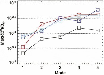
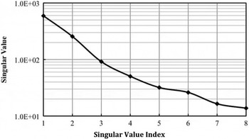
Although only a few sensitivity calculations have been done, there are enough to illustrate that the plasma sensitivities to different external magnetic perturbations can decrease exponentially. Park studied the sensitivity of tokamaks to perturbations that drive magnetic islands (Park et al. Reference Park, Schaffer, Menard and Boozer2007, Reference Park, Boozer, Menard and Schaffer2008), figure 2. Boozer and Ku studied the sensitivity of stellarator neoclassical transport (Ku & Boozer Reference Ku and Boozer2010b ; Boozer & Ku Reference Boozer and Ku2011), figure 3. In both studies, the plasma sensitivity was found to drop essentially exponentially.
Ku & Boozer (Reference Ku and Boozer2010b ) showed that the use of two concepts significantly simplifies the coils required to support a plasma with given physics properties. These concepts were external magnetic fields (1) that can be efficiently produced and (2) to which the plasma is sensitive.
The external magnetic perturbations normalized to the toroidal field required to drive islands in ITER of given width for
 $n=1$
, black;
 $n=2$
, red;
 $n=3$
, blue; and
 $n=4$
, light blue. The calculations included all rational surfaces for three equilibria: inductive, hybrid, and advanced (Park et al.
Reference Park, Boozer, Menard and Schaffer2008).

The singular values associated with the enhancement of the effective ripple of W7-X by all possible external magnetic perturbations were found (Boozer & Ku Reference Boozer and Ku2011) to decay exponentially. The effective ripple (Nemov et al. Reference Nemov, Kasilov, Kernbichler and Heyn1999) is a measure of the enhancement of neoclassical transport.

The concept of plasma sensitivity is closely connected, § 2.2.1 and § 12 of Boozer (Reference Boozer2015), with the theory of plasma optimization. Important optimization topics that will be considered in § 2.2.1 are (1) which physics properties can and cannot be independently optimized and (2) the determination of the most efficient possible external magnetic field that is consistent with a given set of plasma properties.
2.2.1. Stellarator optimization
The basic concepts of the modern strategy for stellarator optimization were initiated in Garching (Chodura et al. Reference Chodura, Dommaschk, Herrnegger, Lotz, Nührenberg and Schlüter1981; Nührenberg & Zille Reference Nührenberg and Zille1988) in the 1980s. The state of a plasma with a definite pressure and current profile is fixed by a choice of the outermost surface (Bauer et al. Reference Bauer, Betancourt and Garabedian1984).
A standard expression for the outermost surface is the Garabedian representation (Bauer et al.
Reference Bauer, Betancourt and Garabedian1984). A Garabedian surface is described in
 $(R_{g},{\it\varphi},Z_{g})$
cylindrical coordinates,
 $\boldsymbol{x}_{g}({\it\theta},{\it\varphi})=R_{g}\hat{\boldsymbol{R}}({\it\varphi})+Z_{g}\hat{\boldsymbol{Z}}$
, by expressing
 $R_{g}({\it\theta},{\it\varphi})$
and
 $Z_{g}({\it\theta},{\it\varphi})$
using complex notation,
 $$\begin{eqnarray}R_{g}+\text{i}Z_{g}=\mathop{\sum }_{mn}{\it\Delta}_{mn}\text{e}^{\text{i}(n{\it\varphi}-(m-1){\it\theta})},\end{eqnarray}$$
where
 $R_{g}$
,
 $Z_{g}$
and
 ${\it\Delta}_{mn}$
are all real. A given set of
 ${\it\Delta}_{mn}$
defines a surface.
An optimized stellarator is found by minimizing a quantity
 ${\it\chi}^{2}$
as a function of the shape parameters
 ${\it\Delta}_{mn}$
. Each physical quantity that is to be optimized has a target value,
 ${\rm\pi}_{{\it\alpha}}^{(target)}$
, and the value
 ${\rm\pi}_{{\it\alpha}}({\it\Delta}_{mn})$
achieved in a plasma state defined by a set of shape parameters
 ${\it\Delta}_{mn}$
. The definition of
 ${\it\chi}^{2}({\it\Delta}_{mn})$
is
 $$\begin{eqnarray}\displaystyle & \displaystyle {\it\chi}^{2}({\it\Delta}_{mn})\equiv \mathop{\sum }_{{\it\alpha}}\frac{{\it\chi}_{{\it\alpha}}^{2}}{{\it\sigma}_{{\it\alpha}}^{2}}, & \displaystyle\end{eqnarray}$$
 $$\begin{eqnarray}\displaystyle & \displaystyle {\it\chi}_{{\it\alpha}}^{2}({\it\Delta}_{mn})\equiv ({\rm\pi}_{{\it\alpha}}({\it\Delta}_{mn})-{\rm\pi}_{{\it\alpha}}^{(target)})^{2}. & \displaystyle\end{eqnarray}$$
 ${\it\sigma}_{{\it\alpha}}$
measure the relative importance of the various measures and ensure consistency of units. The choice of
 ${\it\sigma}_{{\it\alpha}}$
is much of the art of optimization.
The indeterminacy of the weighting
 ${\it\sigma}_{{\it\alpha}}$
of different properties is well known in everyday life. When searching for a new home, a safe neighbourhood, a short commute, comfortable size and low cost are all desirable features, but they cannot all be optimized. Despite agreement on desirable features, their relative weighting in determining the optimal home will vary from family to family.
Each of the
 ${\it\chi}_{{\it\alpha}}^{2}$
represents a simple property. Two that will be used as examples are (1) the effective ripple in the magnetic field strength on a magnetic surface (Nemov et al.
Reference Nemov, Kasilov, Kernbichler and Heyn1999), which is a measure of the enhancement of neoclassical transport, and (2) the resonant current driven on a particular rational magnetic surface due to an ideal MHD perturbation. In a tokamak this current can be calculated by the IPEC code (Park et al.
Reference Park, Schaffer, Menard and Boozer2007) and measures the extent to which that perturbation would drive an island if the resonant current were allowed to relax. A related calculation has been done for stellarators (Nührenberg et al.
Reference Nührenberg, Boozer and Hudson2009). For both examples, the target function is zero.
A third example of a
 ${\it\chi}_{{\it\alpha}}^{2}$
is a method for determining the most efficient external magnetic field consistent with the plasma having a given set of physics properties. Define functions
 ${\rm\pi}_{{\it\alpha}}=\text{e}^{2t_{{\it\alpha}}}{\it\Phi}_{{\it\alpha}}^{2}$
. The
 ${\it\Phi}_{{\it\alpha}}$
are obtained from the external field required to support the equilibrium,
 $\boldsymbol{B}_{x}\boldsymbol{\cdot }\hat{\boldsymbol{n}}({\it\Delta}_{mn})$
, by an expansion in the
 $\boldsymbol{F}_{{\it\alpha}}^{(t)}$
, which are the left eigenvectors of the transfer matrix
 $\unicode[STIX]{x1D64F}$
. To exclude highly inefficient magnetic fields, which have an index greater than
 $i_{c}$
, a
 ${\rm\pi}_{{\it\alpha}}^{2}({\it\Delta}_{mn})$
can be defined by the square of the amplitude of the field components that are to be excluded,
 ${\rm\pi}_{{\it\alpha}}^{2}=\text{e}^{2t_{i_{c}}}\sum _{i>i_{c}}{\it\Phi}_{i}^{2}$
. The code STELLOPT/COILOPT combines the stellarator physics and coil optimization in a single code (Strikler et al.
Reference Strikler, Hirshman, Spong, Cole, Lyon, Nelson, Williamson and Ware2004) but does so by optimizing coefficients in a Fourier representation of the coils. STELLOPT/COILOPT could be modified to optimize in the space of complete and non-redundant set external magnetic fields.
The standard method for calculating stellarator equilibria is the VMEC code (Hirshman & Whitson Reference Hirshman and Whitson1983), and that code coupled with one of many insights tied to the name of Shafranov, the virtual casing principle (Shafranov & Zakharov Reference Shafranov and Zakharov1972), gives the external magnetic field
 $\boldsymbol{B}_{x}\boldsymbol{\cdot }\hat{\boldsymbol{n}}({\it\Delta}_{mn})$
required to support a plasma state defined by a set of
 ${\it\Delta}_{mn}$
. The normal field
 $\boldsymbol{B}_{x}\boldsymbol{\cdot }\hat{n}$
can be expanded in the left eigenfunctions of the transfer matrix to obtain dimensionless amplitude coefficients,
 $$\begin{eqnarray}\displaystyle a_{i}\equiv \frac{1}{B_{0}}\oint \boldsymbol{B}_{x}\boldsymbol{\cdot }\hat{n}F_{i}^{(t)}w\,\text{d}{\it\theta}\,\text{d}{\it\varphi}=\frac{{\it\Phi}_{i}}{B_{0}A}. & & \displaystyle\end{eqnarray}$$
2.2.2. Sensitivity of an optimum
Once an optimum stellarator configuration is found, the
 ${\it\Delta}_{mn}$
can be varied by a small amount,
 ${\it\delta}{\it\Delta}_{mn}$
, away from their optimal values. A small change in the shape of the plasma, a given
 ${\it\delta}{\it\Delta}_{mn}$
, implies a small change in the external magnetic field required to support the plasma equilibrium, which can be expressed as
 ${\it\delta}\boldsymbol{B}_{x}\boldsymbol{\cdot }\hat{\boldsymbol{n}}$
on a fixed toroidal surface just outside the plasma. Writing the external magnetic field as
 ${\it\delta}\boldsymbol{B}_{x}\boldsymbol{\cdot }\hat{\boldsymbol{n}}=w\boldsymbol{f}^{\dagger }\boldsymbol{\cdot }\unicode[STIX]{x1D731}/A$
, (2.5), changes away from the optimum have the form
 $$\begin{eqnarray}{\it\delta}{\it\chi}^{2}=\unicode[STIX]{x1D731}^{\dagger }\boldsymbol{\cdot }\unicode[STIX]{x1D64E}\boldsymbol{\cdot }\unicode[STIX]{x1D731}.\end{eqnarray}$$
 $\unicode[STIX]{x1D64E}$
is the sensitivity matrix and is what is known as the Hessian matrix in optimization theory.
The sensitivity matrix is symmetric, its eigenvalues have real positive values,
 $\text{e}^{s_{i}}$
, and its eigenvectors
 $F_{i}^{(s)}({\it\theta},{\it\varphi})$
can be ordered by the magnitude of the associated eigenvalue – the eigenvector with the largest eigenvalue first.
2.2.3. Sensitivity of individual
 ${\it\chi}_{{\it\alpha}}^{2}$

Each
 ${\it\chi}_{{\it\alpha}}^{2}$
, which is associated with a simple property, has an eigenfunction
 $f_{{\it\alpha}}({\it\theta},{\it\varphi})$
, which gives the unique distribution of external magnetic field
 ${\it\delta}\boldsymbol{B}_{x}\boldsymbol{\cdot }\hat{\boldsymbol{n}}\propto wf_{{\it\alpha}}$
that produces a small change in that property – whether small changes are quadratic or linear in the perturbation amplitude.
The dependence of
 ${\it\chi}_{{\it\alpha}}^{2}$
on the perturbation amplitude can be quadratic, as is the case for the singular current on a particular rational surface in a tokamak. The singular current is proportional to the driving perturbation and has the form
 $I_{{\it\alpha}}=\sum _{i}\unicode[STIX]{x1D61D}_{i}{\it\Phi}_{i}$
, where
 ${\it\alpha}$
denotes a particular rational surface. The matrix
 $\unicode[STIX]{x1D61D}_{i}$
is a matrix vector, which has only one non-zero singular value and that singular value is associated with a particular eigenfunction
 $f_{{\it\alpha}}({\it\theta},{\it\varphi})$
.
Even near a minimum of
 ${\it\chi}^{2}$
, the dependence of a particular
 ${\it\chi}_{{\it\alpha}}^{2}$
can be linear in the perturbation amplitude,
 ${\it\chi}_{{\it\alpha}}^{2}=\sum _{i}\unicode[STIX]{x1D61D}_{i}{\it\Phi}_{i}$
. This occurs when a change in the
 ${\it\Delta}_{mn}$
about the optimum of necessity makes one property better and another worse. The matrix row vector
 $\unicode[STIX]{x1D61D}_{i}$
has only one non-zero singular value, which is associated with a particular eigenfunction
 $f_{{\it\alpha}}({\it\theta},{\it\varphi})$
.
The eigenfunctions
 $f_{{\it\alpha}}({\it\theta},{\it\varphi})$
from different
 ${\it\chi}_{{\it\alpha}}^{2}$
are not generally independent. Indeed, the symmetric matrix
 $\unicode[STIX]{x1D64A}$
of overlap integrals
 $$\begin{eqnarray}\unicode[STIX]{x1D616}_{{\it\alpha}{\it\beta}}\equiv \oint f_{{\it\alpha}}f_{{\it\beta}}w\,\text{d}{\it\theta}\,\text{d}{\it\varphi}\end{eqnarray}$$
must have an eigenvalue that is zero for
 ${\it\chi}_{{\it\alpha}}^{2}$
to have a linear dependence on the perturbation to a plasma state in which
 ${\it\chi}^{2}$
is at a minimum. When the
 $f_{{\it\alpha}}$
from different properties are orthogonal,
 $\unicode[STIX]{x1D616}_{{\it\alpha}{\it\beta}}={\it\delta}_{{\it\alpha}{\it\beta}}$
, and all eigenvalues are unity. The eigenvalues of
 $\unicode[STIX]{x1D64A}$
will be written as
 $\text{e}^{-o_{i}}$
and the eigenfunctions as
 $F_{i}^{(o)}({\it\theta},{\it\varphi})$
. The coupling between two properties,
 ${\it\alpha}$
and
 ${\it\beta}$
, is given by the overlap integral
 $\unicode[STIX]{x1D616}_{{\it\alpha}{\it\beta}}$
between their eigenfunctions.
The number of non-zero eigenvalues of
 $\unicode[STIX]{x1D64A}$
is the number of the functions
 $F_{i}^{(o)}$
that are independent. When an eigenvalue of
 $\unicode[STIX]{x1D64A}$
is small, properties coupled in that eigenfunction are tightly coupled – one cannot be changed without changing another. The weightings
 ${\it\sigma}_{{\it\alpha}}$
in the optimization only determine where in
 ${\it\Delta}_{mn}$
space the
 ${\it\chi}^{2}$
optimized plasma state is located. The choice of the
 ${\it\sigma}_{{\it\alpha}}$
has no direct effect on the coupling between properties, and in particular what types of further optimization of certain properties are possible, in the neighbourhood of that plasma state.
An area in which improved optimization may be important is the confinement of energetic alpha particles. Power loss is not the issue: roughly half the alphas are on passing-particle trajectories, which are well confined when magnetic surfaces exist. The issue is controlling the damage to the wall surrounding the plasma from bombardment by energetic alpha particles. An extremely low rate of alpha loss may not be required. It may be possible to steer the lost alphas into a pool of liquid metal, which would eliminate the material-damage issue.
An important question is how collections of properties can be independently controlled. This question is addressed by the singular value decomposition of the matrix
 $$\begin{eqnarray}\unicode[STIX]{x1D60A}_{ij}\equiv \oint \text{e}^{-t_{i}}F_{i}^{(t)}\text{e}^{-o_{j}}F_{j}^{(o)}w\,\text{d}{\it\theta}\,\text{d}{\it\varphi}.\end{eqnarray}$$
When a singular value
 $\text{e}^{-c_{\ell }}$
is small compared to unity, the right eigenvector
 ${\mathcal{F}}_{k}^{(c)}$
, which is a linear combination of the
 $F_{j}^{(o)}$
can only be driven with low efficiency. When
 $\text{e}^{-c_{\ell }}$
is small compared to other singular values, extreme accuracy is required in the ratio of currents in different coils in order to separately drive this particular collection of properties.
2.3. Applications to coil design
Distance between the plasma and the coils is critical not only to provide space for the blanket and shields but also for an adequate divertor that is consistent with a narrow divertor slot for the plasma states that the device is designed to support, § 3. In addition, the greater the distance between the coils and the plasma the fewer the number of error field distributions to which the plasma has unacceptable sensitivity. For all of these issues, the importance of choosing plasma configurations that not only have good physics properties but also are consistent with efficient magnetic field distributions is clear. Features such as easy access to the plasma chamber are also much easier to design when the coil set need only produce the efficient field distributions. The coils should be designed so the eigenfunctions of the sensitivity matrix
 $\unicode[STIX]{x1D64E}$
with large eigenvalues can be independently controlled. This can be done using trim coils, which by definition produce only a small magnetic field.
2.3.1. Flexibility for many configurations
Once a desirable plasma state is found that requires only efficiently produced external magnetic fields, the optimization of the design for supporting
 $p_{s}\gg 1$
plasma states should be carried out. This can be done by finding the minimal set of efficiently produced distributions
 $n_{x}$
that are required to support a large set of plasma states. The external magnetic fields required to support each of these plasma states can be designated on an envelope toroidal surface, which is defined so it lies outside the plasmas in all of the states but close to a plasma in at least one of the states. Each plasma state
 $p$
has a set of distributions
 ${\mathcal{F}}_{i}^{p}$
of the efficiency-ordered fields on the envelope surface required to support it, with each at an amplitude
 $a_{i}^{p}$
, (2.10). The issue is how many coils that are independently controllable,
 $n_{x}$
, are required to provide most of the required magnetic field to support the
 $p_{s}$
plasma states. The remaining fields are either provided by trim coils or perhaps some parts of the remaining fields are sufficiently small not to require control.
The error in the required magnetic field to support the
 $p\text{th}$
plasma state which is defined by expansion coefficients
 $\boldsymbol{a}_{p}$
, (2.10), can be written as
 $$\begin{eqnarray}{\it\delta}\boldsymbol{B}^{(p)}\boldsymbol{\cdot }\hat{\boldsymbol{n}}=w(\boldsymbol{a}_{p}-\unicode[STIX]{x1D63C}\boldsymbol{\cdot }\boldsymbol{D})^{\dagger }\boldsymbol{\cdot }\boldsymbol{{\mathcal{F}}}^{(t)},\end{eqnarray}$$
where each element in the matrix column vector
 $\boldsymbol{D}$
represents the B-normal distribution on the envelope surface that is produced by a single coil. The matrix
 $\unicode[STIX]{x1D608}_{ij}$
is the amplitude of the
 $i\text{th}$
efficiency-ordered normal field distribution produced by the
 $j\text{th}$
element of
 $\boldsymbol{D}$
. With the basic coils, one wishes to minimize the additional fields that must be supplied by auxiliary coils. That is the coils should be chosen so
 $\boldsymbol{D}$
can be adjusted to minimize the root-mean-square (RMS) error in the normal magnetic field on the control surface. A weighting matrix, such as the sensitivity matrix, can be added, but for simplicity it will be assumed that one wishes to minimize the (RMS) field error
 ${\mathcal{E}}_{p}$
in each of the
 $p_{s}$
plasma states, where
 $$\begin{eqnarray}{\mathcal{E}}_{p}^{2}\equiv (\boldsymbol{a}_{p}-\unicode[STIX]{x1D63C}\boldsymbol{\cdot }\boldsymbol{D})^{\dagger }\boldsymbol{\cdot }(\boldsymbol{a}_{p}-\unicode[STIX]{x1D63C}\boldsymbol{\cdot }\boldsymbol{D}).\end{eqnarray}$$
When
 $\boldsymbol{D}$
is chosen to minimize
 ${\mathcal{E}}_{p}^{2}$
for the
 $p\text{th}$
plasma state,
 $$\begin{eqnarray}\displaystyle & \displaystyle \boldsymbol{D}=\unicode[STIX]{x1D63C}_{s}^{-1}\boldsymbol{\cdot }\boldsymbol{a}_{p}, & \displaystyle\end{eqnarray}$$
 $$\begin{eqnarray}\displaystyle & \displaystyle {\mathcal{E}}_{p}^{2}=\boldsymbol{a}_{p}^{\dagger }\boldsymbol{\cdot }(\unicode[STIX]{x1D64B}^{\dagger }\boldsymbol{\cdot }\unicode[STIX]{x1D64B})\boldsymbol{\cdot }\boldsymbol{a}_{p},\quad \text{where} & \displaystyle\end{eqnarray}$$
 $$\begin{eqnarray}\displaystyle & \displaystyle \unicode[STIX]{x1D64B}\equiv \mathbf{1}-\unicode[STIX]{x1D63C}\boldsymbol{\cdot }\unicode[STIX]{x1D63C}_{s}^{-1}, & \displaystyle\end{eqnarray}$$
 $\mathbf{1}$
is the unit matrix, and
 $\unicode[STIX]{x1D63C}_{s}^{-1}$
is the pseudo-inverse of the matrix
 $\unicode[STIX]{x1D63C}$
.
The pseudo-inverse
 $\unicode[STIX]{x1D63C}_{s}^{-1}$
is defined by SVD, which means the form
 $\unicode[STIX]{x1D63C}=\unicode[STIX]{x1D650}\boldsymbol{\cdot }\unicode[STIX]{x1D668}_{A}\boldsymbol{\cdot }\unicode[STIX]{x1D651}^{\dagger }$
, where
 $\unicode[STIX]{x1D650}^{-1}=\unicode[STIX]{x1D650}^{\dagger }$
,
 $\unicode[STIX]{x1D651}^{-1}=\unicode[STIX]{x1D651}^{\dagger }$
, and
 $\unicode[STIX]{x1D668}_{A}$
is diagonal with all elements greater than or equal to zero. An SVD exists for essentially any matrix. The pseudo-inverse
 $\unicode[STIX]{x1D63C}_{s}^{-1}\equiv \unicode[STIX]{x1D650}\boldsymbol{\cdot }\unicode[STIX]{x1D668}_{{\mathcal{A}}}^{-1}\boldsymbol{\cdot }\unicode[STIX]{x1D651}^{\dagger }$
, where for any diagonal elements
 $(s_{A})_{i}\geqslant s_{min}$
, the element
 $(\unicode[STIX]{x1D668}_{{\mathcal{A}}}^{-1})_{i}\equiv 1/(s_{A})_{i}$
, but if
 $(s_{A})_{i}<s_{min}$
, then
 $(\unicode[STIX]{x1D668}_{{\mathcal{A}}}^{-1})_{i}\equiv 0$
. When
 $s_{min}$
is made smaller, more equilibria can be supported by a given set of coils, but when
 $s_{min}$
is too small, the currents may become too large and accuracy requirements on the currents may be too great to be feasible.
Let
 $i_{x}$
be the number of efficiency-ordered distributions required to support all
 $p_{s}$
plasma states, then
 $\unicode[STIX]{x1D63C}$
is an
 $i_{x}\times i_{D}$
matrix, where
 $i_{D}$
is the number of elements in
 $\boldsymbol{D}$
, which is the number of independent drivable fields in the main coil set. The matrix
 $\unicode[STIX]{x1D63C}$
must have
 $i_{x}-i_{D}$
singular values that are zero, when
 $i_{x}>i_{D}$
. What one wishes to do is to choose the components of
 $\unicode[STIX]{x1D63C}$
for fixed
 $i_{x}$
and
 $i_{D}$
to make the maximum over
 $p$
of
 ${\mathcal{E}}_{p}$
as small as possible.
 ${\mathcal{E}}_{p}$
represents the strength of the field that must be produced by trim coils. When
 ${\mathcal{E}}_{p}$
is too large, either
 $i_{D}$
must be made larger or the range of plasma states reduced.
2.3.2. Error-field mitigation
Reducing deviations of the externally provided magnetic field from the design field by extreme precision of construction increases the cost, time, and the uncertainty of building fusion experiments. These three factors can be minimized by including field error mitigation in the design of an experiment. When the magnetic field errors are too large, too many trim coils are required for practical control and too much current can be required in the trim coils for a practical design. The basic theory of error-field mitigation given here follows § 12.3 of Boozer (Reference Boozer2015) and is related to the theory of machine flexibility, § 2.3.1. The theory of plasma control through modification of the magnetic field distributions to which plasma is sensitive is essentially identical to the theory of error-field mitigation.
The error in the magnetic field
 ${\it\delta}\boldsymbol{B}_{m}$
produced by the main equilibrium coils is determined in the plasma region by the normal component
 ${\it\delta}\boldsymbol{B}_{m}\boldsymbol{\cdot }\hat{\boldsymbol{n}}$
to a control surface just on the plasma side of the coils. That is,
 $$\begin{eqnarray}{\it\delta}\boldsymbol{B}_{m}\boldsymbol{\cdot }\hat{\boldsymbol{n}}=w\mathop{\sum }_{i}{\it\delta}{\it\Phi}_{i}^{(m)}f_{i}({\it\theta}_{c},{\it\varphi}_{c}),\end{eqnarray}$$
where the
 $f_{i}({\it\theta}_{c},{\it\varphi}_{c})$
are an orthonormal set of functions on the coil control surface.
The perturbation to the externally produced field on plasma boundary is then
 $$\begin{eqnarray}{\it\delta}\unicode[STIX]{x1D731}_{x}=\unicode[STIX]{x1D64F}\boldsymbol{\cdot }{\it\delta}\unicode[STIX]{x1D731}_{m}+\unicode[STIX]{x1D648}\boldsymbol{\cdot }\boldsymbol{J},\end{eqnarray}$$
where
 $\unicode[STIX]{x1D64F}$
is a transfer matrix, which relates the magnetic perturbations on the plasma surface to the perturbations near the coils, and
 $\unicode[STIX]{x1D648}$
is a mutual inductance matrix that gives the effect of currents
 $\boldsymbol{J}$
in the control coils.
The plasma sensitivity is measured by
 ${\it\delta}\unicode[STIX]{x1D731}_{x}^{\dagger }\boldsymbol{\cdot }\unicode[STIX]{x1D64E}\boldsymbol{\cdot }{\it\delta}\unicode[STIX]{x1D731}_{x}$
. The currents
 $\boldsymbol{J}$
in the trim coils should be chosen to minimize
 ${\it\delta}\unicode[STIX]{x1D731}_{x}^{\dagger }\boldsymbol{\cdot }\unicode[STIX]{x1D64E}\boldsymbol{\cdot }{\it\delta}\unicode[STIX]{x1D731}_{x}$
. The answer is
 $\unicode[STIX]{x1D648}^{\dagger }\boldsymbol{\cdot }\unicode[STIX]{x1D64E}\boldsymbol{\cdot }\unicode[STIX]{x1D648}\boldsymbol{\cdot }\boldsymbol{J}=-\unicode[STIX]{x1D648}^{\dagger }\boldsymbol{\cdot }S\boldsymbol{\cdot }\unicode[STIX]{x1D64F}\boldsymbol{\cdot }{\it\delta}\unicode[STIX]{x1D731}_{m}$
. The optimal trim-coil currents are then
 $$\begin{eqnarray}\displaystyle & \displaystyle \boldsymbol{J}=-\boldsymbol{{\mathcal{C}}}_{k}\boldsymbol{\cdot }{\it\delta}\unicode[STIX]{x1D731}_{m},\quad \text{ where} & \displaystyle\end{eqnarray}$$
 $$\begin{eqnarray}\displaystyle & \displaystyle \boldsymbol{{\mathcal{C}}}_{k}\equiv (\unicode[STIX]{x1D648}^{\dagger }\boldsymbol{\cdot }\unicode[STIX]{x1D64E}\boldsymbol{\cdot }\unicode[STIX]{x1D648})_{k}^{-1}\boldsymbol{\cdot }\unicode[STIX]{x1D648}^{\dagger }\boldsymbol{\cdot }\unicode[STIX]{x1D64E}\boldsymbol{\cdot }\unicode[STIX]{x1D64F}, & \displaystyle\end{eqnarray}$$
 $k$
means
 $k$
singular values are retained in the pseudoinverse of
 $\unicode[STIX]{x1D648}^{\dagger }\boldsymbol{\cdot }\unicode[STIX]{x1D64E}\boldsymbol{\cdot }\unicode[STIX]{x1D648}$
. When the currents in the trim coils are set optimally, the sensitivity measure is
 $$\begin{eqnarray}\displaystyle & \displaystyle {\it\delta}\unicode[STIX]{x1D731}_{x}^{\dagger }\boldsymbol{\cdot }\unicode[STIX]{x1D64E}\boldsymbol{\cdot }{\it\delta}\unicode[STIX]{x1D731}_{x}={\it\delta}\unicode[STIX]{x1D731}_{m}^{\dagger }\boldsymbol{\cdot }\boldsymbol{{\mathcal{S}}}_{k}\boldsymbol{\cdot }{\it\delta}\unicode[STIX]{x1D731}_{m}, & \displaystyle\end{eqnarray}$$
 $$\begin{eqnarray}\displaystyle & \displaystyle \boldsymbol{{\mathcal{S}}}_{k}\equiv (\unicode[STIX]{x1D64F}-\unicode[STIX]{x1D648}\boldsymbol{\cdot }\boldsymbol{{\mathcal{C}}}_{k})^{\dagger }\boldsymbol{\cdot }\unicode[STIX]{x1D64E}\boldsymbol{\cdot }(\unicode[STIX]{x1D64F}-\unicode[STIX]{x1D648}\boldsymbol{\cdot }\boldsymbol{{\mathcal{C}}}_{k}). & \displaystyle\end{eqnarray}$$
The number of singular values
 $k$
retained in
 $\boldsymbol{{\mathcal{C}}}_{k}$
can be interpreted as the effective number of trim coils that can be used for error-field mitigation. The condition number of
 $\boldsymbol{{\mathcal{C}}}_{k}$
, which is the ratio of the largest to the smallest retained singular values, should be as small as possible since it measures how accurately the coil currents must be chosen to independently control
 $k$
error fields. The required construction accuracy is generally set by having sufficiently few field errors that require mitigation. That is,
 ${\it\delta}\unicode[STIX]{x1D731}_{x}^{\dagger }\boldsymbol{\cdot }\unicode[STIX]{x1D64E}\boldsymbol{\cdot }{\it\delta}\unicode[STIX]{x1D731}_{x}$
must be sufficiently small for a practical value of
 $k$
, where
 $k$
is both the effective number of control coils and the number of error fields requiring correction.
The singular values of
 $\boldsymbol{{\mathcal{C}}}_{k}$
generally increase exponentially from one to the next, so the allowed number of errors that can require correction has a relatively sharp upper limit. It should be noted that neither
 $\boldsymbol{{\mathcal{S}}}_{k}$
nor
 $\boldsymbol{{\mathcal{C}}}_{k}$
has a dependence on the actual magnetic field errors, so an error-field mitigation system can be designed without knowing the as-built coil errors. Once an error-field mitigation system is designed, the largest tolerable as-built errors can be determined both in magnitude and form.
3. Divertors
Divertors are considered necessary for particle handling on fusion-grade toroidal plasmas. The primary purpose of a divertor is to concentrate the region on the wall in which the plasma particle exhaust occurs so that pumps can be installed at this location. Covering the whole wall with pumps is not practical.
Although concentrating the particle exhaust is advantageous, concentrating the plasma energy exhaust is not. It is generally assumed that most of the power can be radiated. Indeed, the radiated power may become sufficiently large that the plasma recombines before it has contact with the surrounding structures, which is called a detached divertor. Of course the flow velocity of the particles from the plasma must remain sufficiently high that, as plasma crosses the edge of the confinement region, the particles are swept into the region in which they are to be pumped.
The first question that must be addressed in the design of a divertor is what are the desirable features. Some of these are as follows. (1) A significant spatial separation between the region of good plasma confinement and the footpoints of the divertor field lines on the surrounding structures. This separation makes it more difficult for sputtered particles to enter the plasma volume and gives room for the beneficial loss of power by radiation. (2) A location for a slot for field lines to pass into a divertor chamber that is independent of the plasma state. (3) A controlled spreading of the heat load. The intersection locations on the wall for field lines that lie just outside the confinement region tend to be sharp, but spreading of the heat flux is exponentially sensitive to diffusion when neighbouring magnetic field lines have a significant exponentiation of their separation.
The optimization of the physics properties of stellarators was originally carried out at Garching without provision for a divertor. Nevertheless, by 1992 divertor designs for optimized stellarators were being published by Strumberger (Reference Strumberger1992), Nührenberg & Strumberger (Reference Nührenberg and Strumberger1992).
As noted by Nührenberg (Reference Nührenberg2006), stellarators typically have sharp edges, which locally are similar to the X-point of a tokamak divertor: ‘optimized stellarators have similar flux surface shape, so in particular, they exhibit helical edges along which field lines beyond the last closed magnetic surface are preferentially diverted’.
A sharp edge on a magnetic surface must be a magnetic field line. At a sharp edge, one component of the curvature of the surface goes to infinity. Ampere’s law implies that the current required to produce a magnetic field must be no further away than of order one over the curvature of the field lines. The implication is that a sharp edge cannot be crossed by a magnetic field line.
Unlike the tokamak, the sharp edges on the surface of a stellarator are (1) helical and (2) need not continue around the full torus. Although the sharp edges on the surface of a stellarator cannot be crossed by magnetic field lines, they need not enforce a value of the transform
 ${\it\iota}$
when they do not encircle the entire torus.
3.1. Divertor issues
The first step in designing a divertor for a stellarator is the choice of the basic magnetic configuration. Methods of determining the freedom and the basic consequences of choices are discussed in this paper. Once the choice of the basic magnetic configuration is made, additional studies are required to answer questions such as where pumps and baffle plates should be located. These choices are made using codes, such as the EMC3-EIRENE code (Feng et al. Reference Feng, Sardei, Kisslinger and Grigull1997, Reference Feng, Frerichs, Kobayashi, Bader, Effenberg, Harting, Hoelbe, Huang, Kawamura and Lore2014), but such codes are not an efficient method to determine the available choices for the basic magnetic configuration.
In non-axisymmetric systems, knowledge is remarkably limited on the boundary between a region in which magnetic field lines form nested magnetic surfaces and confine a plasma and a region in which magnetic field lines strike the surrounding walls and form a divertor. Knowledge is required on what types of divertors are feasible for stellarators, especially stellarators that can have a strong net plasma current, such as quasi-symmetric stellarators.
Magnetic field lines are the trajectories of a one-and-a-half degree of freedom Hamiltonian,
 ${\it\psi}_{p}({\it\psi}_{t},{\it\theta},{\it\varphi})$
, § 3.3. The boundary issues that need to be understood to improve stellarator design are also important to a broader field of physics, and the literature of that broader field is relevant to divertor design.
As discussed in § 3.3, the behaviour of magnetic field lines in the boundary region can be studied by adding a non-Hamiltonian term to the magnetic field line trajectories, which causes the lines to spiral outwards at a rate
 $D_{s}$
. As
 $D_{s}\rightarrow 0$
, field line trajectories are sampled in regions of confining magnetic surfaces as well as in annuli of stochastic field lines that can lie between annuli of nested surfaces. When
 $D_{s}>0$
, any magnetic field line trajectory eventually strikes the walls. The
 $D_{s}\rightarrow 0$
limit provides a definition of both the outermost confining magnetic surface and the first escaping magnetic field lines.
When many magnetic field lines are followed, the first escaping magnetic field lines form flux tubes. That is, magnetic field lines do not escape from the vicinity of the last confining flux surface at all locations – only at certain locations – and it is the properties of these first escaping flux tubes that define the basic properties of divertors. Questions are as follows.
-
(1) Where do the trajectories of the first escaping flux tubes go? Divertor plates could in principle be located at any location along, and with any degree of tangency to, these trajectories.
-
(2) Can the trajectories of the first escaping flux tubes be made insensitive to the currents in the plasma? Can divertor plates be located to provide satisfactory performance for a range of plasma states?
-
(3) How is the amount of flux in the first escaping flux tubes affected by field line diffusion? Magnetic field lines do not diffuse, but plasma following those field lines does. The behaviour of the diffusing plasma can be studied by introducing magnetic field line diffusion.
-
(4) How are the properties of the first escaping flux tubes affected by (i) how well the outermost confining surface approximates a magnetic surface with sharp edges, (ii) the finite length of the sharp edges, (iii) the rotational transform of the magnetic field lines of the outermost confining surface, and (iv) the effective transform of sharp-edge segments?
3.2. Generalizations of tokamak divertors
Modern tokamaks have divertors that are characterized by an X-point, which is actually a circular sharp edge, or X-line, along which the poloidal magnetic field vanishes. The separatrix is the toroidal magnetic surface that includes the X-line. Magnetic field lines enclosed by the separatrix encircle the plasma while those outside strike the walls.
Divertors on axisymmetric tokamaks can be thought of in two ways, which become distinct in stellarators, and will be called resonant and non-resonant divertors.
3.2.1. Resonant divertors
In a resonant divertor, the external magnetic field has a resonance on an outer magnetic surface that has a rotational transform
 ${\it\iota}_{d}$
. In a tokamak, the resonance is
 ${\it\iota}_{d}=0$
, and the magnetic island that forms is axisymmetric. The W7-X stellarator has a resonant divertor; the resonance is
 ${\it\iota}_{d}=5/5$
, which means that the external magnetic field has five periods toroidally and has a component that has five periods poloidally. The
 $5/5$
component splits the
 ${\it\iota}=5/5$
surface to form a magnetic island, which diverts the magnetic field lines (Strumberger Reference Strumberger1996; Feng et al.
Reference Feng, Sardei, Grigull, McCormick, Kisslinger and Reiter2006). The same divertor plate locations can be used if the resonant surface is chosen to be at
 ${\it\iota}_{d}=5/6$
or
 ${\it\iota}_{d}=5/4$
.
The advantages of a magnetic-island or resonant divertor are that (1) the divertor region is compact staying very close to the body of the plasma and (2) the divertor has a long connection length because of the slowness with which magnetic field lines encircle a narrow island.
The resonant divertor has the following two disadvantages.
-
(1) The formation of a magnetic island requires a fixed resonant rotational transform
${\it\iota}_{d}$
be maintained at the plasma edge, which is difficult when the plasma evolution naturally has a large variation in the net toroidal current. -
(2) The intersection points of the magnetic field lines with the surrounding structure in a resonant divertor are separated by only a small distance from the main plasma body, despite the many toroidal transits required by a magnetic field line to go from the plasma edge to the surrounding structure.

3.2.2. Non-resonant divertors
A non-resonant divertor is produced by using the external magnetic field to force a sharp edge on the plasma surface. The axisymmetric sharp edge on the surface of a tokamak, the X-line, cannot be crossed by a magnetic field line, which forces the rotational transform to be zero on the separatrix. This is despite the fact that the toroidal current enclosed by the separatrix produces a poloidal field that, away from the X-line, would be associated with a rotational transform
 ${\it\iota}\sim 1/3$
.
The magnetic field lines near a sharp edge, even an edge that is just a segment of a line, resemble those near at tokamak X-line. That is, magnetic field lines are carried off to the walls, and non-resonant terms in the magnetic field line Hamiltonian, when sufficiently large, can produce a divertor configuration. Non-resonant divertors have been discussed for quasi-axisymmetric stellarators (Mioduszewski et al. Reference Mioduszewski, Owen, Spong, Fenstermacher, Koniges, Rognlien, Umansky, Grossman and Kugel2007; Mau et al. Reference Mau, Kaiser, Grossman, Raffray, Want, Lyon, Maingi, Ku and Zarnstorff2008).
Few studies have been made of non-resonant stellarator divertors, but, as in a tokamak, a non-resonant divertor can be insensitive to the net plasma current, and the diverted field lines can intersect the divertor structures far from the main plasma body.
Sharp edges are a requirement for a non-resonant divertor but may or may not be present in a resonant divertor. Sharp edges are present in the W7-X resonant divertor. Nevertheless, an island for a resonant divertor can be located on what would otherwise be a smooth though rational magnetic surface. That is, the location of the place from which field lines are diverted can be determined either by the global geometry defining sharp edges, as in a non-resonant divertor, or by a particular rational value of the rotational transform
 ${\it\iota}_{d}$
, as in resonant divertor.
3.3. Hamiltonian method for studying divertors
The primary constraint on magnetic field line behaviour is the Hamiltonian nature of magnetic field line trajectories, see Kerst (Reference Kerst1962), Boozer (Reference Boozer1983), and § 5.1 of Boozer (Reference Boozer2015). The use of this constraint allows general studies to be carried out of the behaviour of magnetic field lines near the plasma edge.
The behaviour of magnetic field lines can be separated, § 5.1 of Boozer (Reference Boozer2015), into a position vector
 $\boldsymbol{x}_{p}({\it\psi}_{t},{\it\theta},{\it\varphi})$
and a magnetic field line Hamiltonian
 ${\it\psi}_{p}({\it\psi}_{t},{\it\theta},{\it\varphi})$
, which contains the topological information on field lines,
 $\text{d}{\it\psi}_{t}/\text{d}{\it\varphi}=-\partial {\it\psi}_{p}/\partial {\it\theta}$
and
 $\text{d}{\it\theta}/\text{d}{\it\varphi}=\partial {\it\psi}_{p}/\partial {\it\psi}_{t}$
. This separation is implied by the general representation of a magnetic field
 $2{\rm\pi}\boldsymbol{B}=\boldsymbol{{\rm\nabla}}{\it\psi}_{t}\times \boldsymbol{{\rm\nabla}}{\it\theta}+\boldsymbol{{\rm\nabla}}{\it\varphi}\times \boldsymbol{{\rm\nabla}}{\it\psi}_{p}({\it\psi}_{t},{\it\theta},{\it\varphi})$
in a torus, where
 ${\it\psi}_{t}$
is the toroidal magnetic flux enclosed by a constant-
 ${\it\psi}_{t}$
surface and
 ${\it\psi}_{p}$
is within a sign the poloidal magnetic flux outside a constant-
 ${\it\psi}_{p}$
surface, § 5.1 of Boozer (Reference Boozer2015). The poloidal and toroidal angles
 ${\it\theta}$
and
 ${\it\varphi}$
can be chosen for convenience.
As discussed in § 3.1, the most important issues revolve around the behaviour of the first escaping flux tubes. The flux tubes can be found (Punjabi & Boozer Reference Punjabi and Boozer2014) by modifying the field line equations to
 $\text{d}{\it\psi}_{t}/\text{d}{\it\varphi}=D{\it\psi}_{t}-\partial {\it\psi}_{p}/\partial {\it\theta}$
and
 $\text{d}{\it\theta}/\text{d}{\it\varphi}=\partial {\it\psi}_{p}/\partial {\it\psi}_{t}$
, which causes the field lines to spiral outwards when
 $D=D_{s}$
, where
 $D_{s}>0$
is a constant. The properties of first escaping flux tubes can be obtained by following a large number of trajectories started in the region of good surfaces in the limit as
 $D_{s}\rightarrow 0$
.
 $D$
can also be chosen to have the form
 $D=\pm D_{d}$
, which causes the magnetic field lines to diffuse. Diffusion is very slow compared to spiralling and has a reasonable numerical efficiency only when field lines can be started just inside the last confining magnetic surface.
In the limit as the spiralling coefficient goes to zero,
 $D_{s}\rightarrow 0$
, the first escaping flux tubes contain an infinitesimal magnetic flux, which can be interpreted as a magnetic field line. This follows from the theory of turnstiles in Hamiltonian systems, which was recently reviewed by Meiss (Reference Meiss2015). These flux tubes or field lines have definite trajectories through space and can strike the surrounding walls at any angle from tangential, which implies a helical stripe, to normal, which implies a point. When the flux tube is truly infinitesimal, it will always strike the walls at points – one point per flux tube – but when the flux tube has a finite dimension due either to a non-zero
 $D_{s}$
or more physically to finite diffusion
 $D_{d}$
, the strike points partially fill in a helical segment: the closer to tangential interception the better the helical segment is filled. For two examples with different diffusion coefficients see figure 6 in Strumberger (Reference Strumberger1992). Basic features of divertors, resonant and non-resonant, are determined by the behaviour of these flux tubes, both their trajectories and the extent of their broadening in the presence of diffusion, and the tangency of the divertor structures to these tubes.
Without diffusion, non-axisymmetric perturbations to a tokamak divertor modify the sharp circular interceptions of the field lines just outside the last confining magnetic surface into complicated lobe-like patterns called tangles. Nonetheless, the footpoint locations lie on sharp curves (Poincare Reference Poincaré1899; Evans et al.
Reference Evans, Roeder, Carter and Rapoport2004, Reference Evans, Yu, Jakubowski, Schmitz, Watkins and Moyer2009; Boozer Reference Boozer2015). These curves develop a diffusive width in the presence of a
 $D=\pm D_{d}$
, and the width can be very sensitive to the magnitude of
 $D_{d}$
. Such effects can be efficiently studied using the methods that have been outlined (Punjabi & Boozer Reference Punjabi and Boozer2014).
In order to study the behaviour of magnetic field lines using a model Hamiltonian two functions must be specified: a Hamiltonian
 ${\it\psi}_{p}({\it\psi}_{t},{\it\theta},{\it\varphi})$
and a position vector
 $\boldsymbol{x}_{p}({\it\psi}_{t},{\it\theta},{\it\varphi})$
, which is required to plot the trajectories of the magnetic field line Hamiltonian in ordinary space.
3.4. Model Hamiltonian for magnetic field lines
In the region of the divertor, the magnetic field is generally close to being curl free, so the Hamiltonian chosen for topology studies should be consistent with this requirement. The magnetic field line Hamiltonian that is chosen for the model is
 $$\begin{eqnarray}\displaystyle & \displaystyle {\it\psi}_{p}=\bar{{\it\psi}}_{p}({\it\psi}_{t})+{\it\delta}{\it\psi}_{p}({\it\psi}_{t},{\it\theta},{\it\varphi}), & \displaystyle\end{eqnarray}$$
 $$\begin{eqnarray}\displaystyle & \displaystyle {\it\delta}{\it\psi}_{p}\equiv {\it\psi}_{c}\mathop{\sum }_{m,n}{\it\alpha}_{mn}\left(\frac{{\it\psi}_{t}}{{\it\psi}_{c}}\right)^{m/2}\cos (n{\it\varphi}-m{\it\theta}), & \displaystyle\end{eqnarray}$$
 $$\begin{eqnarray}\displaystyle & \displaystyle \bar{{\it\iota}}({\it\psi}_{t})\equiv \frac{\text{d}\bar{{\it\psi}_{p}}}{\text{d}{\it\psi}_{t}}; & \displaystyle\end{eqnarray}$$
 ${\it\psi}_{c}$
and
 ${\it\alpha}_{mn}$
are constants. The
 ${\it\psi}_{t}^{m/2}$
dependence for the Fourier terms in
 ${\it\psi}_{p}$
is what is expected if the magnetic field is curl free and the
 ${\it\varphi}$
dependence is weak,
 $R_{a}/n\gg {\it\Delta}_{0,0}$
. The terms with
 $m>0$
are due to currents outside the spatial location being considered and the terms with
 $m<0$
are due to currents inside. Only
 $\cos (n{\it\varphi}-m{\it\theta})$
terms are retained because
 $\sin (n{\it\varphi}-m{\it\theta})$
terms break stellarator symmetry, which is the non-axisymmetric generalization of top–bottom symmetry in a tokamak. Stellarator symmetry is not required but is a common simplifying constraint.
3.5. Model position vector
3.5.1. Position vector for resonant divertors
The behaviour of the boundary between confined and non-confined magnetic field lines in a resonant divertor is essentially described by the magnetic field line Hamiltonian, (3.1), and only a moderate number of the constants
 ${\it\alpha}_{mn}$
need be non-zero. The position vector can be chosen to be an extrapolated Garabedian surface, (2.7),
 $\boldsymbol{x}_{p}({\it\psi}_{t},{\it\theta},{\it\varphi})=R\hat{\boldsymbol{R}}+Z\hat{\boldsymbol{Z}}$
, where
 $$\begin{eqnarray}R+\text{i}Z=\mathop{\sum }_{m,n}{\it\Delta}_{mn}\left(\frac{{\it\psi}_{t}}{{\it\psi}_{c}}\right)^{m/2}\text{e}^{\text{i}(n{\it\varphi}-(m-1){\it\theta})}.\end{eqnarray}$$
3.5.2. Position vector for non-resonant divertors
The position vector and the Garabedian surface, (2.7), have fundamentally different roles in the modelling of non-resonant versus resonant divertors. For non-resonant divertors, the position vector can be chosen to have a simple form. The Garabedian surface determines the constants that appear in the magnetic field line Hamiltonian. A field line of the Hamiltonian should coincide with the Garabedian surface. That is,
 $\boldsymbol{x}_{p}({\it\psi}_{t}={\it\psi}_{g},{\it\theta},{\it\varphi})$
must equal
 $\boldsymbol{x}_{g}({\it\theta},{\it\varphi})$
for some choice of the function
 ${\it\psi}_{g}({\it\theta},{\it\varphi})$
.
A consistent position vector can be defined using ordinary
 $(R,{\it\varphi},Z)$
cylindrical coordinates,
 $\boldsymbol{x}_{p}({\it\psi}_{t},{\it\theta},{\it\varphi})=R({\it\psi}_{t},{\it\theta},{\it\varphi})\hat{\boldsymbol{R}}({\it\varphi})+Z({\it\psi}_{t},{\it\theta},{\it\varphi})\hat{\boldsymbol{Z}}$
. The
 $R$
and
 $Z$
positions are real but can be defined by the complex form
 $$\begin{eqnarray}R+\text{i}Z=R_{a}({\it\varphi})+\text{i}Z_{a}({\it\varphi})+{\it\Delta}_{0,0}\sqrt{\frac{{\it\psi}_{t}}{{\it\psi}_{c}}}\text{e}^{\text{i}({\it\theta}+{\it\delta}{\it\theta})},\end{eqnarray}$$
where the constant
 ${\it\psi}_{c}$
is a characteristic value of the toroidal flux and
 ${\it\Delta}_{0,0}$
, a constant from the Garabedian representation, is the minor radius. The function
 ${\it\delta}{\it\theta}({\it\psi}_{t},{\it\theta},{\it\varphi})$
is required for the equation
 $\boldsymbol{x}_{p}({\it\psi}_{g},{\it\theta},{\it\varphi})=\boldsymbol{x}_{g}({\it\theta},{\it\varphi})$
to have a solution for the toroidal magnetic flux
 ${\it\psi}_{t}={\it\psi}_{g}({\it\theta},{\it\varphi})$
on the Garabedian surface, (2.7). The equation for the axis of the poloidal angle is
 $$\begin{eqnarray}R_{a}+\text{i}Z_{a}=\mathop{\sum }_{n=0}^{\infty }{\it\Delta}_{1,n}\text{e}^{\text{i}n{\it\varphi}}.\end{eqnarray}$$
3.6. Non-resonant divertor model
3.6.1. Expressions for
${\it\psi}_{g}$
and
${\it\delta}{\it\theta}$


The position vector defined in (3.5) is consistent with the Garabedian position vector, (2.7), only when the functions
 ${\it\psi}_{g}({\it\theta},{\it\varphi})$
and
 ${\it\delta}{\it\theta}({\it\theta},{\it\varphi})$
have a certain form.
The equation
 $\boldsymbol{x}_{p}({\it\psi}_{g},{\it\theta},{\it\varphi})=\boldsymbol{x}_{g}({\it\theta},{\it\varphi})$
, where
 ${\it\psi}_{t}={\it\psi}_{g}({\it\theta},{\it\varphi})$
on the Garabedian surface, implies
 $$\begin{eqnarray}\sqrt{\frac{{\it\psi}_{g}}{{\it\psi}_{c}}}\text{e}^{\text{i}{\it\delta}{\it\theta}}=\mathop{\sum }_{m\neq 0}\frac{{\it\Delta}_{m,n}}{{\it\Delta}_{0,0}}\text{e}^{\text{i}(n{\it\varphi}-m{\it\theta})}.\end{eqnarray}$$
This equation for
 ${\it\psi}_{g}({\it\theta},{\it\varphi})$
and
 ${\it\delta}{\it\theta}({\it\theta},{\it\varphi})$
can be solved by letting
 $$\begin{eqnarray}\displaystyle & \displaystyle C({\it\theta},{\it\varphi})\equiv 1+{\it\Sigma}^{\prime }\frac{{\it\Delta}_{m,n}}{{\it\Delta}_{0,0}}\cos (n{\it\varphi}-m{\it\theta}), & \displaystyle\end{eqnarray}$$
 $$\begin{eqnarray}\displaystyle & \displaystyle S({\it\theta},{\it\varphi})\equiv {\it\Sigma}^{\prime }\frac{{\it\Delta}_{m,n}}{{\it\Delta}_{0,0}}\sin (n{\it\varphi}-m{\it\theta}), & \displaystyle\end{eqnarray}$$
 ${\it\Sigma}^{\prime }$
means that the terms
 $(m,n)$
equal to
 $(0,0)$
and
 $(1,n)$
are omitted from the sum. One finds that
 $$\begin{eqnarray}\displaystyle & \displaystyle \cos {\it\delta}{\it\theta}=\frac{C}{\sqrt{C^{2}+S^{2}}}, & \displaystyle\end{eqnarray}$$
 $$\begin{eqnarray}\displaystyle & \displaystyle \sin {\it\delta}{\it\theta}=\frac{S}{\sqrt{C^{2}+S^{2}}}, & \displaystyle\end{eqnarray}$$
 $$\begin{eqnarray}\displaystyle & \displaystyle {\it\psi}_{g}({\it\theta},{\it\varphi})=(C^{2}+S^{2}){\it\psi}_{c}. & \displaystyle\end{eqnarray}$$
The Fourier expansions of
 ${\it\psi}_{g}/{\it\psi}_{c}$
and
 ${\it\delta}{\it\theta}$
have the general forms
 $$\begin{eqnarray}\displaystyle & \displaystyle \frac{{\it\psi}_{g}}{{\it\psi}_{c}}=1+2{\it\delta}({\it\theta},{\it\varphi}), & \displaystyle\end{eqnarray}$$
 $$\begin{eqnarray}\displaystyle & \displaystyle {\it\delta}\equiv {\it\Sigma}^{\prime }{\it\delta}_{m,n}\cos (n{\it\varphi}-m{\it\theta}), & \displaystyle\end{eqnarray}$$
 $$\begin{eqnarray}\displaystyle & \displaystyle {\it\delta}{\it\theta}={\it\Sigma}^{\prime }{\it\theta}_{mn}\sin (n{\it\varphi}-m{\it\theta}). & \displaystyle\end{eqnarray}$$
 $|{\it\Delta}_{mn}/{\it\Delta}_{00}|$
that appear in the sum
 ${\it\Sigma}^{\prime }$
are small, both
 ${\it\delta}_{mn}$
and
 ${\it\theta}_{mn}$
are approximated by
 ${\it\Delta}_{mn}/{\it\Delta}_{00}$
.
3.6.2. Consistency of the Hamiltonian with the Garabedian surface
On the Garabedian surface, (2.7), the toroidal flux coordinate that appears in the standard position vector is
 ${\it\psi}_{t}={\it\psi}_{g}({\it\theta},{\it\varphi})$
. The constraint that the Garabedian surface be a magnetic surface implies
 $$\begin{eqnarray}\frac{\text{d}{\it\psi}_{t}}{\text{d}{\it\varphi}}=\frac{\partial {\it\psi}_{g}}{\partial {\it\theta}}\frac{\text{d}{\it\theta}}{\text{d}{\it\varphi}}+\frac{\partial {\it\psi}_{g}}{\partial {\it\varphi}}\end{eqnarray}$$
when evaluated on the Garabedian surface
 ${\it\psi}_{t}={\it\psi}_{g}$
. This equation and Hamilton’s equations imply
 $$\begin{eqnarray}\frac{\partial {\it\psi}_{g}}{\partial {\it\theta}}\left(\frac{\partial {\it\psi}_{p}}{\partial {\it\psi}_{t}}\right)_{g}+\left(\frac{\partial {\it\psi}_{p}}{\partial {\it\theta}}\right)_{g}+\frac{\partial {\it\psi}_{g}}{\partial {\it\varphi}}=0.\end{eqnarray}$$
The required derivatives of the magnetic field line Hamiltonian are
 $$\begin{eqnarray}\displaystyle & \displaystyle \left(\frac{\partial {\it\psi}_{p}}{\partial {\it\psi}_{t}}\right)_{g}=\bar{{\it\iota}}_{g}+\mathop{\sum }_{m,n}\frac{m}{2}{\it\alpha}_{mn}(1+2{\it\delta})^{(m-2)/2}\cos (\cdots \,), & \displaystyle\end{eqnarray}$$
 $$\begin{eqnarray}\displaystyle & \displaystyle \bar{{\it\iota}}_{g}=\bar{{\it\iota}}\big({\it\psi}_{a}(1+2{\it\delta})\big), & \displaystyle\end{eqnarray}$$
 $$\begin{eqnarray}\displaystyle & \displaystyle \left(\frac{\partial {\it\psi}_{p}}{\partial {\it\theta}}\right)_{g}={\it\psi}_{a}\mathop{\sum }_{m,n}m{\it\alpha}_{mn}(1+2{\it\delta})^{m/2}\sin (\cdots \,),\hspace{14.45377pt} & \displaystyle\end{eqnarray}$$
 $$\begin{eqnarray}\displaystyle & \displaystyle \frac{\partial {\it\psi}_{t}^{g}}{\partial {\it\theta}}=2{\it\psi}_{a}{\it\Sigma}^{\prime }m{\it\delta}_{mn}\sin (n{\it\varphi}-m{\it\theta}), & \displaystyle\end{eqnarray}$$
 $$\begin{eqnarray}\displaystyle & \displaystyle \frac{\partial {\it\psi}_{t}^{g}}{\partial {\it\varphi}}=-2{\it\psi}_{a}{\it\Sigma}^{\prime }n{\it\delta}_{mn}\sin (n{\it\varphi}-m{\it\theta}), & \displaystyle\end{eqnarray}$$
 $\cos (\cdots \,)=\cos (n{\it\varphi}-m{\it\theta})$
. The Fourier terms that are approximately field line resonant are the ones that are most important to control.
The solution to (3.17) for a set of
 ${\it\alpha}_{mn}$
can be found by an optimization technique. Optimization algorithms are made more efficient when given an approximate optimum. An approximate optimum can be found by assuming that all of the Garabedian shape coefficients
 $|{\it\Delta}_{mn}/{\it\Delta}_{0,0}|$
that appear in the sum
 ${\it\Sigma}^{\prime }$
are small, then
 $$\begin{eqnarray}{\it\alpha}_{mn}\approx 2\frac{n-\bar{{\it\iota}}_{g}m}{m}\frac{{\it\Delta}_{m,n}}{{\it\Delta}_{00}},\end{eqnarray}$$
where
 $\bar{{\it\iota}}_{g}=\bar{{\it\iota}}({\it\psi}_{g})\approx \bar{{\it\iota}}({\it\psi}_{c})$
. Note that the toroidal flux dependence of the model Hamiltonian must be
 ${\it\psi}_{t}^{m/2}$
not
 ${\it\psi}_{t}^{|m/2|}$
to obtain a general solution for
 ${\it\alpha}_{mn}$
.
3.6.3. Removing islands
As discussed in § 3.1, it is important to be able to investigate the behaviour of non-resonant divertors in the limit as the last confining magnetic surface closer approximates a magnetic surface with sharp edges. To carry out this study, it is necessary to have a way to remove magnetic islands by adjusting the
 ${\it\alpha}_{mn}$
. A procedure for doing this can be based on a method developed by Greene (Reference Greene1979).
Greene’s method for eliminating islands in a canonical-coordinate region has three elements: (1) find the closed field line trajectories, called fixed points, of the Hamiltonian
 ${\it\psi}_{p}({\it\psi}_{t},{\it\theta},{\it\varphi})$
; (2) construct the mapping matrix
 $\unicode[STIX]{x1D648}$
for trajectories near a fixed point; (3) adjust the appropriate coefficient
 ${\it\alpha}_{mn}$
in the Hamiltonian until the trace of
 $\unicode[STIX]{x1D648}$
equals 2.
(i) Find the fixed points. The trajectories of the model Hamiltonian, (3.1), are top–bottom symmetric in the primary cross-sections,
 ${\it\varphi}=0,{\rm\pi}$
. Letting
 $x\equiv \sqrt{{\it\psi}_{t}}\cos {\it\theta}$
be the horizontal and
 $y\equiv \sqrt{{\it\psi}_{t}}\sin {\it\theta}$
the vertical coordinate in a primary cross-section, the fixed points are located along the
 $x$
axis. To find fixed points, integrate from the starting point
 $(x=x_{0},y=0)$
at
 ${\it\varphi}=0$
to
 ${\it\varphi}=2{\rm\pi}M$
, where the number of toroidal transits
 $M$
is an integer, to obtain
 $x_{M}(x_{0})$
and
 $y_{M}(x_{0})$
. A necessary condition for an
 $M\text{th}$
-order fixed point is that
 $y_{M}(x_{0})$
change sign as
 $x_{0}$
is varied, with the fixed point located at the place where
 $y_{M}(x_{0})=0$
.
To obtain closure at an
 $M\text{th}$
-order fixed point, the field line trajectory advances from
 ${\it\theta}=0$
to
 ${\it\theta}=2{\rm\pi}N$
with
 $N$
an integer. The rotational transform of the magnetic field line that passes through the fixed point is
 ${\it\iota}_{f}=N/M$
.
(ii) Construct the near fixed-point map. Close to a fixed point of order
 $M$
, the trajectory map for going from
 ${\it\varphi}=0$
to
 ${\it\varphi}=2{\rm\pi}M$
has the form
 $$\begin{eqnarray}\left(\begin{array}{@{}c@{}}{\it\delta}x_{k+1}\\ {\it\delta}y_{k+1}\end{array}\right)=\unicode[STIX]{x1D648}\boldsymbol{\cdot }\left(\begin{array}{@{}c@{}}{\it\delta}x_{k}\\ {\it\delta}y_{k}\end{array}\right),\end{eqnarray}$$
where
 ${\it\delta}x_{k}$
is the
 $k\text{th}$
iterate of the horizontal distance,
 $x-x_{f}$
, of the field line from the fixed point, and
 ${\it\delta}y_{k}$
the vertical distance from the fixed point, and the integer
 $k$
is given by
 $kM$
being the number of toroidal transits.
The matrix is constructed by following two trajectories neighbouring the fixed point from
 ${\it\varphi}=0$
to
 ${\it\varphi}=2{\rm\pi}M$
. The first has the starting point
 $({\it\delta}x_{1},0)$
and ends at
 $({\it\delta}x_{11},{\it\delta}y_{12})$
, the second has the starting point
 $(0,{\it\delta}y_{2})$
and ends at
 $({\it\delta}x_{21},{\it\delta}y_{22})$
. Neighbouring means
 $|{\it\delta}x_{1}|\rightarrow 0$
and
 $|{\it\delta}y_{2}|\rightarrow 0$
. The mapping matrix is
 $$\begin{eqnarray}\unicode[STIX]{x1D648}=\left(\begin{array}{@{}c@{}}\displaystyle \frac{{\it\delta}x_{11}}{{\it\delta}x_{1}}\displaystyle \frac{{\it\delta}y_{12}}{{\it\delta}x_{1}}\\ \displaystyle \frac{{\it\delta}x_{21}}{{\it\delta}y_{2}}\displaystyle \frac{{\it\delta}y_{22}}{{\it\delta}y_{2}}\end{array}\right).\end{eqnarray}$$
The matrix
 $\unicode[STIX]{x1D648}$
should have a unit determinant,
 $D\equiv M_{11}M_{22}-M_{12}M_{21}=1$
, since the magnetic field line Hamiltonian is area preserving. The trace,
 $T\equiv M_{11}+M_{22}$
, will be the important quantity and will have an error
 ${\sim}|\sqrt{D}-1|$
.
(iii) Greene’s trace condition. To understand Greene’s trace condition that the trace must equal 2 to eliminate islands, first note that the trace
 $T$
and determinant
 $D$
give the eigenvalues of a
 $2\times 2$
matrix. That is, the matrix
 $\unicode[STIX]{x1D648}$
can be written in the form
 $\unicode[STIX]{x1D648}=\unicode[STIX]{x1D64B}\boldsymbol{\cdot }{\bf\mu}\boldsymbol{\cdot }\unicode[STIX]{x1D64B}^{-1}$
, where
 ${\bf\mu}$
is diagonal with its two diagonal elements,
 ${\it\mu}_{\pm }=T/2\pm \sqrt{(T/2)^{2}-D}$
, the eigenvalues. For the mapping matrix,
 $D=1$
. As
 $T\rightarrow 2$
, the two eigenvalues are
 ${\it\mu}_{\pm }=1\pm \sqrt{T-2}$
.
When the near fixed point mapping is iterated
 $k$
times, the mapping matrix
 $\unicode[STIX]{x1D648}_{k}$
is a
 $k$
-fold product of the matrix
 $\unicode[STIX]{x1D648}$
, so
 $\unicode[STIX]{x1D648}_{k}=\unicode[STIX]{x1D64B}\boldsymbol{\cdot }{\bf\mu}_{k}\boldsymbol{\cdot }\unicode[STIX]{x1D64B}^{-1}$
where the diagonal elements of
 ${\bf\mu}_{k}$
are
 ${\it\mu}_{k\pm }=({\it\mu}_{\pm })^{k}=\text{e}^{\pm k\sqrt{T-2}}$
as
 $T\rightarrow 2$
. When
 $T>2$
, the trajectories exponentiate away from the fixed point, so the fixed point is the X-point of an island. When
 $T<2$
, the trajectories orbit the fixed point, so the fixed point is the O-point of an island. Only when
 $T=2$
can the fixed point lie on a magnetic surface.
4. Summary
The tokamak is a simpler concept and can produce impressive levels of plasma confinement even without the subtlety of design that requires a supercomputer. Nevertheless, the path to a fusion reactor using the tokamak requires large experiments with uncertain outcomes because a burning tokamak plasma is in a nonlinear, self-organized state, which is both difficult to predict and to control.
The path to a fusion reactor using the stellarator requires a computational program to design an attractive candidate, and relatively modest experiments for validation and to address uncertainties of physics, such as the possibility of impurity accumulation. The reactor issues for stellarators that cannot be addressed in moderate size experiments are materials issues, which must be faced by the fusion program whether a fusion reactor is based on a tokamak or a stellarator. Even in that area, the stellarator may have a fundamental advantage of easier maintenance access to the highly irradiated components.
A computational program based on concepts explained in this paper could establish whether stellarators could be made far more attractive for fusion applications than is apparent from existing designs. Judging from the level of computational effort required to develop the W7-X configuration, the cost of a program would be small, perhaps
 ${\sim}10^{-3}$
of the cost of just building ITER: computations are very inexpensive compared to experiments. Rational program planning depends on such calculations being done as quickly as possible.
Acknowledgements
This material is based upon work supported by the US Department of Energy, Office of Science, Office of Fusion Energy Sciences under Award no. DE-FG02-95ER54333. The author thanks M. Landreman for his many questions and enlightening calculations related to magnetic field efficiency.