1 Introduction
Dynamo action, i.e. the self-amplification of a magnetic field by the flow of an electrically conducting fluid, is considered to be the main mechanism for the generation of the magnetic fields of stars and planets (Moffatt Reference Moffatt1978). In order to gain a better understanding of the processes at play, different experimental groups have investigated dynamo action (Peffley, Cawthorne & Lathrop Reference Peffley, Cawthorne and Lathrop2000; Nornberg et al. Reference Nornberg, Spence, Kendrick, Jacobson and Forest2006; Frick et al. Reference Frick, Noskov, Denisov and Stepanov2010; Colgate et al. Reference Colgate, Beckley, Si, Martinic, Westpfahl, Slutz, Westrom, Klein, Schendel, Scharle, McKinney, Ginanni, Bentley, Mickey, Ferrel, Li, Pariev and Finn2011) but so far only three experiments have been successful: Gailitis et al. (Reference Gailitis, Lielausis, Dement’ev, Platacis and Cifersons2000), Stieglitz & Müller (Reference Stieglitz and Müller2001), Monchaux et al. (Reference Monchaux, Berhanu, Bourgoin, Odier, Moulin, Pinton, Volk, Fauve, Mordant, Pétrélis, Chiffaudel, Daviaud, Dubrulle, Gasquet, Marié and Ravelet2007). These three experiments were all performed in liquid sodium. The first two experiments used optimized flows guided by pipes that intentionally limited the influence that turbulence could have on the dynamo process. The experimentalists found dynamo action with a magnetic field having a shape corresponding to the one predicted by using kinematic dynamo computations based on analytical flows. The third dynamo has been observed in the von Kármán sodium experiment (VKS) located in Cadarache: in 2006 experimentalists observed a magnetic field generated by a turbulent flow produced by two counter-rotating impellers in a cylindrical vessel. It has been found that both the geometry and the material composing the impellers play crucial roles in the dynamo action threshold: for example, at fixed available mechanical power, dynamo action occurs only when at least one of the rotating impellers is made of soft iron (Miralles et al. Reference Miralles, Bonnefoy, Bourgoin, Odier, Pinton, Plihon, Verhille, Boisson, Daviaud and Dubrulle2013). When the two soft iron impellers counter-rotate at the same angular velocity, another puzzling observation is that the generated magnetic field is statistically steady and mainly axisymmetric with an axial dipole and a strong azimuthal component located near the impellers (Boisson et al. Reference Boisson, Aumaitre, Bonnefoy, Bourgoin, Daviaud, Dubrulle, Odier, Pinton, Plihon and Verhille2012). This magnetic field could not be predicted by using simplified axisymmetric geometries and velocity fields averaged in azimuth and time: kinematic dynamo simulations usually give an equatorial dipole superimposed with two anti-parallel vertical magnetic structures near the vessel axis (see e.g. Ravelet et al. Reference Ravelet, Chiffaudel, Daviaud and Léorat2005, Laguerre et al. Reference Laguerre, Nore, Léorat and Guermond2006, Marié, Normand & Daviaud Reference Marié, Normand and Daviaud2006, Gissinger et al. Reference Gissinger, Iskakov, Fauve and Dormy2008, Guermond et al. Reference Guermond, Léorat, Luddens, Nore and Ribeiro2011a ).
It is clear that the nature of the material composing the impellers greatly influences the transmission conditions enforced on the magnetic field, and that the geometry of the impellers controls the dynamics of the tip vortices generated between the blades (Ravelet et al. Reference Ravelet, Dubrulle, Daviaud and Ratié2012; Kreuzahler et al. Reference Kreuzahler, Schulz, Homann, Ponty and Grauer2014). But a precise experimental investigation of the influences of the material properties and the blade geometry is not feasible due to the lack of accurate techniques such as non-intrusive Gaussmeters or PIV measurements in liquid metals. It is natural then to turn to computer simulations to gain some insight into the VKS experiment. The objective of the present work is to report on three-dimensional numerical simulations of the von Kármán sodium experiment at high kinetic Reynolds numbers. Dynamo action is obtained with a magnetic field that is mainly axisymmetric and similar to the one observed in the experiment. Some of these results were announced in Nore et al. (Reference Nore, Castanon Quiroz, Cappanera and Guermond2016), but in the present paper we go well beyond the range of kinetic Reynolds numbers attained in the above reference. Our main result is that the critical magnetic Reynolds number decreases as the kinetic Reynolds number increases and this number seems to converge to a constant at very large kinetic Reynolds numbers. We also confirm that, everything else being fixed, the critical magnetic Reynolds number decreases as the magnetic permeability of the impellers increases.
The paper is organized as follows. The set-up of the 2006 VKS2 experiment together with the relevant parameters is shortly presented in § 2. The governing equations and the numerical methods that are used to solve them are also briefly described. Section 3 presents hydrodynamical simulations performed for a large range of kinetic Reynolds numbers. Dynamo action is studied in § 4. The impact of the relative magnetic permeability of the impellers and of the boundary conditions is studied. The dynamo threshold is determined for a large range of kinetic Reynolds numbers; it decreases as the kinetic Reynolds number increases and it seems to reach an asymptotic value for very large kinetic Reynolds numbers. The structure of the generated magnetic field shows a striking similarity with the one observed in the VKS2 experiment in all of the cases investigated. Key ingredients for dynamo action in the VKS2 set-up are identified in § 5. It is shown in particular in this section that kinematic dynamo computations using the time-averaged velocity field computed at high fluid Reynolds number give a non-axisymmetric magnetic field similar to the one obtained from simplified time-averaged and azimuthally averaged velocity field, but this dynamo is very different from the one observed in VKS2 experiment. Concluding remarks are reported in § 6 and a tentative scenario is proposed.
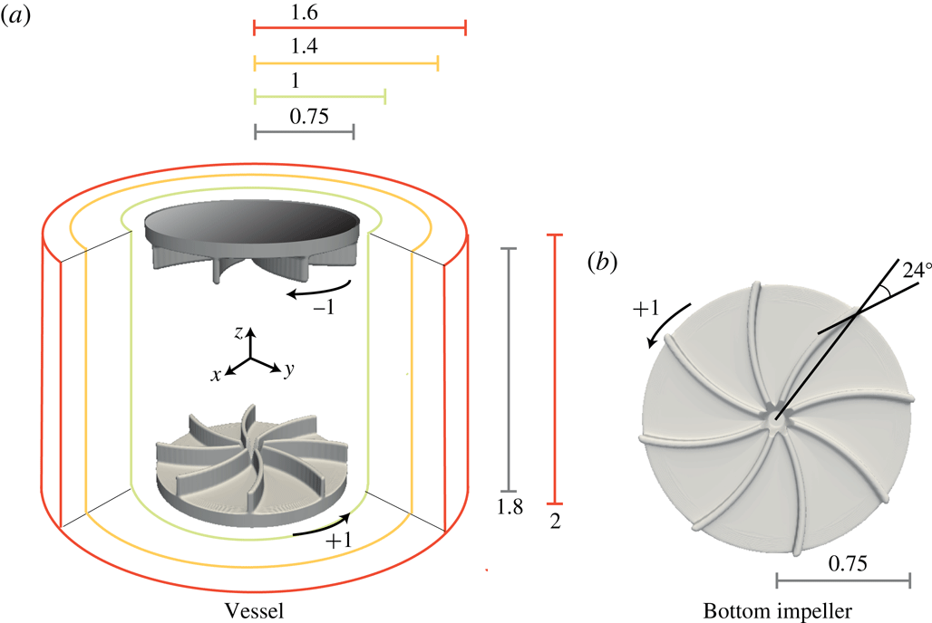
Schematic of the VKS2 experimental device of Monchaux et al. (Reference Monchaux, Berhanu, Bourgoin, Odier, Moulin, Pinton, Volk, Fauve, Mordant, Pétrélis, Chiffaudel, Daviaud, Dubrulle, Gasquet, Marié and Ravelet2007) in non-dimensional units. The impellers counter-rotate as indicated in (a) and are fitted with eight curved blades (b).

2 Technical preliminaries
In the present paper we simulate numerically the VKS2 experiment with the flow driven by the TM73 impellers (see figure 1 and Monchaux et al. (Reference Monchaux, Berhanu, Bourgoin, Odier, Moulin, Pinton, Volk, Fauve, Mordant, Pétrélis, Chiffaudel, Daviaud, Dubrulle, Gasquet, Marié and Ravelet2007)). We begin by describing the geometry. Then we present the governing equations and the algorithms that are used in our magnetohydrodynamic (MHD) code (Guermond et al. Reference Guermond, Laguerre, Léorat and Nore2007, Reference Guermond, Laguerre, Léorat and Nore2009, Reference Guermond, Léorat, Luddens, Nore and Ribeiro2011a ).
2.1 Experimental set-up and data
The VKS2 set-up described in Monchaux et al. (Reference Monchaux, Berhanu, Bourgoin, Odier, Moulin, Pinton, Volk, Fauve, Mordant, Pétrélis, Chiffaudel, Daviaud, Dubrulle, Gasquet, Marié and Ravelet2007) uses two concentric cylindrical containers: the first one has a very small thickness and is of radius
 $R_{cyl}=206~\text{mm}$
; the second one is thick and made of copper, its inner radius is
 $R_{in}=289~\text{mm}$
and its outer radius is
 $R_{out}=330~\text{mm}$
. Both containers have a total height
 $H=412~\text{mm}$
. The impellers are located at the two extremities of the inner container. There is some fluid behind the impellers in the experiment, but in the present simulations we neglect this fluid layer. The impellers are composed of two disks each supporting eight blades. The disks have radius
 $R_{b}=155~\text{mm}$
and are
 $20~\text{mm}$
thick. The blades have height
 $41~\text{mm}$
, thickness
 $5~\text{mm}$
, and the angle of curvature is equal to
 $24^{\circ }$
. The distance between the inner faces of the disks is set to
 $370~\text{mm}$
so that the aspect ratio of the cylindrical fluid domain is
 $370/206=1.8$
. The fluid contained in the inner vessel is pushed by the convex side of the blades. A schematic representation of the experimental set-up is shown in figure 1 using
 $R_{cyl}$
as reference length scale.
The vessel contains approximately 150 l of liquid sodium heated at
 $120\,^{\circ }\text{C}$
. The kinematic viscosity is
 $\unicode[STIX]{x1D708}=6.78\times 10^{-7}~\text{m}^{2}~\text{s}^{-1}$
, the density is
 $\unicode[STIX]{x1D70C}=932~\text{kg}~\text{m}^{-3}$
and the electrical conductivity is
 $\unicode[STIX]{x1D70E}=9.6\times 10^{6}~\text{S}~\text{m}^{-1}$
. The corresponding magnetic Prandtl number is
 $P_{m}=\unicode[STIX]{x1D707}_{0}\unicode[STIX]{x1D70E}\unicode[STIX]{x1D708}=0.82\times 10^{-5}$
. The impellers counter-rotate at a frequency
 $f$
, the experimental range of frequencies necessary for observing dynamo action is
 $16~\text{Hz}\leqslant f\leqslant 22~\text{Hz}$
, leading to kinetic Reynolds numbers in the range
 $6.3\times 10^{6}\leqslant R_{e}=2\unicode[STIX]{x03C0}fR_{cyl}^{2}/\unicode[STIX]{x1D708}\leqslant 8.7\times 10^{6}$
and magnetic Reynolds numbers in the range
 $52\leqslant R_{m}^{c}=\unicode[STIX]{x1D707}_{0}\unicode[STIX]{x1D70E}2\unicode[STIX]{x03C0}fR_{cyl}^{2}\leqslant 71$
.
At maximum available mechanical power, a dynamo has been observed with soft iron impellers (made of ferromagnetic material of relative magnetic permeability of the order of 50, see Verhille et al. (Reference Verhille, Plihon, Bourgoin, Odier and Pinton2010)) but not with stainless steel ones (Miralles et al. Reference Miralles, Bonnefoy, Bourgoin, Odier, Pinton, Plihon, Verhille, Boisson, Daviaud and Dubrulle2013).
2.2 Spectral/finite element code for Maxwell and Navier–Stokes equations (SFEMaNS)
To investigate the hydrodynamic and magnetohydrodynamic regimes of the above experimental set-up, we use a code henceforth referred to in this paper as SFEMaNS. This code uses a hybrid spatial discretization combining spectral and finite elements. In a nutshell the code uses a Fourier decomposition in the azimuthal direction and the continuous Hood–Taylor Lagrange elements
 $\mathbb{P}_{1}$
–
 $\mathbb{P}_{2}$
for the pressure and velocity fields in the meridian section. Modulo the computations of nonlinear terms with the fast Fourier transform (FFT), the linear problems for each Fourier mode in the meridian section are uncoupled and are thereby easily parallelized by using the message passing interface (MPI). The solution of the linear problems in the meridian section is further parallelized by using graph partitioning techniques from the METIS library (Karypis & Kumar Reference Karypis and Kumar1998) for the domain decomposition, and subroutines from the portable extensible toolkit for scientific computation library (PETSc) (Balay et al.
Reference Balay, Abhyankar, Adams, Brown, Brune, Buschelman, Eijkhout, Gropp, Kaushik, Knepley, McInnes, Rupp, Smith and Zhang2014) for the linear algebra. For the magnetic part, the algorithm solves the problem using the magnetic induction,
 $\boldsymbol{B}$
, in the conducting region (after standard elimination of the electric field) and the scalar magnetic potential in the insulating exterior. The fields in each region are approximated by using
 $H^{1}$
-conforming Lagrange elements with a penalty technique to control the divergence of
 $\boldsymbol{B}$
in a negative Sobolev norm that guarantees convergence under minimal regularity (see details in Giesecke et al. (Reference Giesecke, Nore, Stefani, Gerbeth, Léorat, Luddens and Guermond2010, § 3.2), Bonito & Guermond (Reference Bonito and Guermond2011), Bonito, Guermond & Luddens (Reference Bonito, Guermond and Luddens2013)). The coupling between conducting and insulating media is done by using an interior penalty method. SFEMaNS has been thoroughly validated on numerous manufactured solutions and against other MHD codes (see e.g. Guermond et al.
Reference Guermond, Laguerre, Léorat and Nore2009; Giesecke et al.
Reference Giesecke, Nore, Stefani, Gerbeth, Léorat, Herreman, Luddens and Guermond2012; Nore et al.
Reference Nore, Zaidi, Bouillault, Bossavit and Guermond2016). The reader who is familiar with the numerical details or is not interested in such details is now invited to jump to § 3.
2.3 Governing equations
Let us now go into some details about the equations that are actually solved in SFEMaNS. The MHD equations are solved in non-dimensional form as follows:
 $$\begin{eqnarray}\displaystyle \unicode[STIX]{x2202}_{t}\boldsymbol{u} & = & \displaystyle -(\unicode[STIX]{x1D735}\times \boldsymbol{u})\times \boldsymbol{u}+\frac{1}{R_{e}}\unicode[STIX]{x0394}\boldsymbol{u}-\unicode[STIX]{x1D735}p+\boldsymbol{f},\end{eqnarray}$$
 $$\begin{eqnarray}\displaystyle \unicode[STIX]{x2202}_{t}\boldsymbol{B} & = & \displaystyle \unicode[STIX]{x1D735}\times (\boldsymbol{u}\times \boldsymbol{B})-\frac{1}{R_{m}}\unicode[STIX]{x1D735}\times \left(\frac{1}{\unicode[STIX]{x1D70E}_{r}}\unicode[STIX]{x1D735}\times \left(\frac{1}{\unicode[STIX]{x1D707}_{r}}\boldsymbol{B}\right)\right),\end{eqnarray}$$
 $$\begin{eqnarray}\displaystyle \unicode[STIX]{x1D735}\boldsymbol{\cdot }\,\boldsymbol{u} & = & \displaystyle 0,\end{eqnarray}$$
 $$\begin{eqnarray}\displaystyle \unicode[STIX]{x1D735}\boldsymbol{\cdot }\,\boldsymbol{B} & = & \displaystyle 0,\end{eqnarray}$$
 $\boldsymbol{u}$
is the velocity field,
 $\boldsymbol{B}$
the magnetic induction field (with the magnetic field
 $\boldsymbol{H}=\boldsymbol{B}/\unicode[STIX]{x1D707}_{0}\unicode[STIX]{x1D707}_{r}$
),
 $p$
the pressure field and
 $\unicode[STIX]{x1D70E}_{r}$
,
 $\unicode[STIX]{x1D707}_{r}$
are the relative conductivity and permeability of the various materials present. The Navier–Stokes and the Maxwell equations are coupled by the Lorentz force
 $\boldsymbol{f}=(\unicode[STIX]{x1D735}\times \boldsymbol{H})\times \boldsymbol{B}$
.
In the present situation the reference length
 $L_{ref}$
is set to
 $R_{cyl}$
. The computational domain for the hydrodynamic study is
 $\unicode[STIX]{x1D6FA}=\{(r,\unicode[STIX]{x1D703},z)\in [0,1]\times [0,2\unicode[STIX]{x03C0})\times [-1,1]\}$
. The computational domain for the MHD study is the larger cylinder
 $\unicode[STIX]{x1D6FA}\cup \unicode[STIX]{x1D6FA}_{out}$
with
 $\unicode[STIX]{x1D6FA}_{out}=\{(r,\unicode[STIX]{x1D703},z)\in [1,1.6]\times [0,2\unicode[STIX]{x03C0})\times [-1,1]\}$
(the geometric dimensions and sketches of the set-up are shown in figures 6
c and 19
b). Denoting by
 $\unicode[STIX]{x1D70E}_{0}$
the electrical conductivity of the liquid sodium,
 $\unicode[STIX]{x1D70C}$
its density and
 $\unicode[STIX]{x1D707}_{0}$
the magnetic permeability of vacuum, the magnetic induction is made non-dimensional by using the Alfvén scaling
 $B=U\sqrt{\unicode[STIX]{x1D70C}\unicode[STIX]{x1D707}_{0}}$
, with
 $U=\unicode[STIX]{x1D714}R_{cyl}$
where
 $\unicode[STIX]{x1D714}$
is the angular velocity of the impellers. The two governing parameters are
 $R_{m}=\unicode[STIX]{x1D707}_{0}\unicode[STIX]{x1D70E}_{0}R_{cyl}^{2}\unicode[STIX]{x1D714}$
, the magnetic Reynolds number, and
 $R_{e}=R_{cyl}^{2}\unicode[STIX]{x1D714}/\unicode[STIX]{x1D708}$
, the kinetic Reynolds number, with
 $\unicode[STIX]{x1D708}$
the kinematic viscosity of the fluid.
Note that the parameters
 $\unicode[STIX]{x1D70E}_{r}$
,
 $\unicode[STIX]{x1D707}_{r}$
are not constant since the walls and the impellers are made of different materials such as copper, steel and soft iron. Specifically, we take
 $\unicode[STIX]{x1D70E}_{r}=1,\unicode[STIX]{x1D707}_{r}=1$
in the region
 $\{(r,\unicode[STIX]{x1D703},z)\in [1,1.4]\times [0,2\unicode[STIX]{x03C0})\times [-1,1]\}$
to represent the lateral layer of stagnant liquid sodium, and
 $\unicode[STIX]{x1D70E}_{r}=4.5,\unicode[STIX]{x1D707}_{r}=1$
in
 $\{(r,\unicode[STIX]{x1D703},z)\in [1.4,1.6]\times [0,2\unicode[STIX]{x03C0})\times [-1,1]\}$
to model the lateral copper wall. The computational domain is slightly smaller than the actual VKS2 container: it does not contain the so-called lid layers, which have been shown in kinematic dynamo simulations to be detrimental to dynamo action, Stefani et al. (Reference Stefani, Xu, Gerbeth, Ravelet, Chiffaudel, Daviaud and Léorat2006), Laguerre et al. (Reference Laguerre, Nore, Léorat and Guermond2006). In the induction equation (2.1b
) we take
 $\boldsymbol{u}_{|\unicode[STIX]{x1D6FA}_{out}}=0$
. With the exception of § 4.3 where we study the impact of the so-called vacuum boundary condition, in the entire paper we impose the perfect ferromagnetic boundary condition
 $\boldsymbol{H}\times \boldsymbol{n}=0$
at the boundary of the computational domain. We shall also refer to this condition as the pseudo-vacuum boundary condition. This boundary condition allows us to save memory and CPU time.
2.4 Moving domains
To distinguish the liquid sodium from the impellers, the cylinder
 $\unicode[STIX]{x1D6FA}$
is split into a solid domain
 $\unicode[STIX]{x1D6FA}_{solid}(t)$
(composed of the rotating impellers) and a fluid domain
 $\unicode[STIX]{x1D6FA}_{fluid}(t)$
, and we introduce the characteristic function
 $\unicode[STIX]{x1D712}$
defined in cylindrical coordinates by:
 $$\begin{eqnarray}\displaystyle \unicode[STIX]{x1D712}(r,\unicode[STIX]{x1D703},z,t)=\left\{\begin{array}{@{}ll@{}}1 & \text{if }(r,\unicode[STIX]{x1D703},z)\in \unicode[STIX]{x1D6FA}_{fluid}(t),\\ 0 & \text{if }(r,\unicode[STIX]{x1D703},z)\in \unicode[STIX]{x1D6FA}_{solid}(t).\end{array}\right. & & \displaystyle\end{eqnarray}$$
In our case
 $\unicode[STIX]{x1D712}=0$
in the impellers (see figure 1). Note that both
 $\unicode[STIX]{x1D6FA}_{solid}(t)$
and
 $\unicode[STIX]{x1D6FA}_{fluid}(t)$
are time dependent. It is not possible to find a frame of reference where these domains are time independent since the impellers move with opposite angular velocities. The ensuing main difficulty is to approximate the Navier–Stokes equations in a time- and
 $\unicode[STIX]{x1D703}$
-dependent domain and to force the velocity in the solid domain
 $\unicode[STIX]{x1D6FA}_{solid}(t)$
to be that of two solid bodies in rotation. This is achieved by using a prediction–correction method of Guermond & Shen (Reference Guermond and Shen2004) and a pseudo-penalty technique of Pasquetti, Bwemba & Cousin (Reference Pasquetti, Bwemba and Cousin2008). Let
 $\unicode[STIX]{x1D70F}$
be the time step and let us generically denote by
 $f^{n}$
the approximation of
 $f(n\unicode[STIX]{x1D70F})$
. The velocity is then updated by using the following scheme:
 $$\begin{eqnarray}\displaystyle & & \displaystyle \frac{3\boldsymbol{u}^{n+1}}{2\unicode[STIX]{x1D70F}}-\frac{1}{R_{e}}\unicode[STIX]{x0394}\boldsymbol{u}^{n+1}=-\unicode[STIX]{x1D735}p^{n}+(1-\unicode[STIX]{x1D712}^{n+1})\frac{3\boldsymbol{u}_{obst}^{n+1}}{2\unicode[STIX]{x1D70F}}\nonumber\\ \displaystyle & & \displaystyle \qquad +\,\unicode[STIX]{x1D712}^{n+1}\left(\frac{4\boldsymbol{u}^{n}-\boldsymbol{u}^{n-1}}{2\unicode[STIX]{x1D70F}}-\unicode[STIX]{x1D735}\left(\frac{4\unicode[STIX]{x1D713}^{n}-\unicode[STIX]{x1D713}^{n-1}}{3}\right)-(\unicode[STIX]{x1D735}\times \boldsymbol{u}^{\ast ,n+1})\times \boldsymbol{u}^{\ast ,n+1}+\boldsymbol{f}^{n+1}\right),\end{eqnarray}$$
where
 $\boldsymbol{u}^{\ast ,n+1}=2\boldsymbol{u}^{n}-\boldsymbol{u}^{n-1}$
and, using cylindrical coordinates,
 $\boldsymbol{u}_{obs}$
is the velocity of the disks and blades defined for all
 $n\geqslant 0$
by:
 $$\begin{eqnarray}\displaystyle \boldsymbol{u}_{obs}^{n}(r,\unicode[STIX]{x1D703},z)=\left\{\begin{array}{@{}ll@{}}-r\boldsymbol{e}_{\unicode[STIX]{x1D703}} & \text{if }z>0,\\ r\boldsymbol{e}_{\unicode[STIX]{x1D703}} & \text{if }z\leqslant 0.\end{array}\right. & & \displaystyle\end{eqnarray}$$
The pressure increment
 $\unicode[STIX]{x1D713}^{n+1}$
is obtained by solving the following Poisson problem:
 $$\begin{eqnarray}\displaystyle \unicode[STIX]{x0394}\unicode[STIX]{x1D713}^{n+1}=\frac{3}{2\unicode[STIX]{x1D70F}}\unicode[STIX]{x1D735}\boldsymbol{\cdot }\,\boldsymbol{u}^{n+1}. & & \displaystyle\end{eqnarray}$$
The pressure is finally updated as follows:
 $$\begin{eqnarray}\displaystyle p^{n+1}=p^{n}+\unicode[STIX]{x1D713}^{n+1}-\frac{1}{R_{e}}\unicode[STIX]{x1D735}\boldsymbol{\cdot }\,\boldsymbol{u}^{n+1}. & & \displaystyle\end{eqnarray}$$
Note that the velocity and the pressure are solutions of the Navier–Stokes equations when
 $\unicode[STIX]{x1D712}=1$
, i.e. in the fluid domain
 $\unicode[STIX]{x1D6FA}_{fluid}(t)$
. When
 $\unicode[STIX]{x1D712}=0$
, i.e. in
 $\unicode[STIX]{x1D6FA}_{solid}(t)$
, the momentum equation reduces to
 $3\boldsymbol{u}^{n+1}/2\unicode[STIX]{x1D70F}-(1/R_{e})\unicode[STIX]{x0394}\boldsymbol{u}^{n+1}=-\unicode[STIX]{x1D735}p^{n}+3\boldsymbol{u}_{obst}^{n+1}/2\unicode[STIX]{x1D70F}$
; to first order in
 $\unicode[STIX]{x1D70F}$
, the solution is
 $\boldsymbol{u}=\boldsymbol{u}_{obs}+O(\unicode[STIX]{x1D70F}/R_{e})$
. Note that the higher the kinetic Reynolds number, the more accurate the method. There are two situations for the initialization of the above algorithm. Either we start from rest, and in this case all the quantities required at
 $n=0$
are set to zero, or we restart from a previous computation, and in this case all the quantities required to restart are taken from the previous computation.
The second difficulty we face is that the material properties in the computational frame depend on the azimuthal angle and time due to the presence of the rotating blades. This is not a serious issue for the conductivity
 $\unicode[STIX]{x1D70E}_{r}$
since the conductivity of the impellers and the liquid sodium are not very different; for the sake of simplicity we take
 $\unicode[STIX]{x1D70E}_{r}=1$
in the impellers and in the liquid sodium. But to account for the heterogeneities of the magnetic permeability, we allow
 $\unicode[STIX]{x1D707}_{r}$
to depend on all the space and time variables, i.e.
 $\unicode[STIX]{x1D707}_{r}=\unicode[STIX]{x1D707}_{r}(r,\unicode[STIX]{x1D703},z,t)$
. More precisely, letting
 $\unicode[STIX]{x1D707}_{r}^{imp}$
be the relative permeability of the impellers and recalling that
 $\unicode[STIX]{x1D707}_{r}=1$
in the liquid sodium, we set
 $$\begin{eqnarray}\displaystyle \unicode[STIX]{x1D707}_{r}(r,\unicode[STIX]{x1D703},z,t)=\unicode[STIX]{x1D712}(r,\unicode[STIX]{x1D703},z,t)+(1-\unicode[STIX]{x1D712}(r,\unicode[STIX]{x1D703},z,t))\unicode[STIX]{x1D707}_{r}^{imp}. & & \displaystyle\end{eqnarray}$$
In order to make the linear algebra in the induction equation time independent, and to avoid the nonlinearity in
 $\unicode[STIX]{x1D703}$
induced by the product
 $(1/\unicode[STIX]{x1D707}_{r})\boldsymbol{B}$
, we split the diffusion term by setting
 $\boldsymbol{B}/\unicode[STIX]{x1D707}_{r}=\boldsymbol{B}/\widetilde{\unicode[STIX]{x1D707}_{r}}+(\boldsymbol{B}/\unicode[STIX]{x1D707}_{r}-\boldsymbol{B}/\widetilde{\unicode[STIX]{x1D707}_{r}})$
, where
 $\widetilde{\unicode[STIX]{x1D707}_{r}}(r,z)$
is defined by
 $\widetilde{\unicode[STIX]{x1D707}_{r}}(r,z):=\min _{0\leqslant \unicode[STIX]{x1D703}<2\unicode[STIX]{x03C0}}\unicode[STIX]{x1D707}_{r}(r,\unicode[STIX]{x1D703},z,t)$
. The first part of the decomposition,
 $\boldsymbol{B}/\widetilde{\unicode[STIX]{x1D707}_{r}}$
, is made implicit while the second part,
 $(\boldsymbol{B}/\unicode[STIX]{x1D707}_{r}-\boldsymbol{B}/\widetilde{\unicode[STIX]{x1D707}_{r}})$
, is made explicit by using
 $\boldsymbol{B}^{\ast ,n+1}=2\boldsymbol{B}^{n}-\boldsymbol{B}^{n-1}$
and
 $\unicode[STIX]{x1D707}_{r}=\unicode[STIX]{x1D707}_{r}^{n+1}$
. The magnetic induction field is therefore updated as follows:
 $$\begin{eqnarray}\displaystyle & & \displaystyle \frac{3\boldsymbol{B}^{n+1}}{2\unicode[STIX]{x1D70F}}+\frac{1}{R_{m}}\unicode[STIX]{x1D735}\times \left(\frac{1}{\unicode[STIX]{x1D70E}_{r}}\unicode[STIX]{x1D735}\times \left(\frac{\boldsymbol{B}^{n+1}}{\widetilde{\unicode[STIX]{x1D707}_{r}}}\right)\right)=\frac{4\boldsymbol{B}^{n}-\boldsymbol{B}^{n-1}}{2\unicode[STIX]{x1D70F}}\nonumber\\ \displaystyle & & \displaystyle \qquad +\,\unicode[STIX]{x1D735}\times (\boldsymbol{u}^{n+1}\times \boldsymbol{B}^{\ast ,n+1})-\frac{1}{R_{m}}\unicode[STIX]{x1D735}\times \left(\frac{1}{\unicode[STIX]{x1D70E}_{r}}\unicode[STIX]{x1D735}\times \left(\boldsymbol{B}^{\ast ,n+1}\left(\frac{1}{\unicode[STIX]{x1D707}_{r}}-\frac{1}{\widetilde{\unicode[STIX]{x1D707}_{r}}}\right)\right)\right).\end{eqnarray}$$
The function
 $\widetilde{\unicode[STIX]{x1D707}_{r}}$
being independent of the azimuth, implicit FFT convolutions are completely avoided. Note also that for each Fourier mode, the linear problem in (2.8) is decoupled from the other Fourier modes. The scheme (2.8) is stable, owing to the condition
 $\widetilde{\unicode[STIX]{x1D707}_{r}}\leqslant \unicode[STIX]{x1D707}_{r}$
, and it can be shown to be second-order accurate in time, see Castanon Quiroz (Reference Castanon Quiroz2015) for details. Finally, the solenoidal constraint (2.1d
) is enforced as in Guermond et al. (Reference Guermond, Léorat, Luddens, Nore and Ribeiro2011a
).
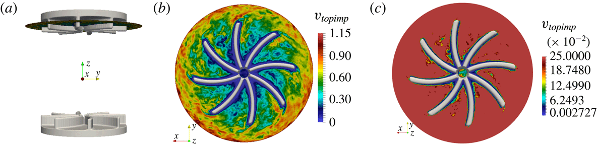
To illustrate the performance of the penalty method, we show in figure 2 some isovalues of the function
 $\unicode[STIX]{x1D712}$
and the amplitude of the velocity field in the reference frame of the top impeller at some arbitrary time at
 $R_{e}=10^{5}$
. Figure 2(a) shows the isovalue
 $\unicode[STIX]{x1D712}=0.75$
in grey and the cutting plane at
 $z=0.8$
. The actual boundary of the blades corresponds to
 $\unicode[STIX]{x1D712}=0.99$
; therefore, the isovalue
 $\unicode[STIX]{x1D712}=0.75$
is inside the blades. Figure 2(b) shows
 $\Vert \boldsymbol{u}-\boldsymbol{u}_{top\text{-}impeller}\Vert$
in the plane
 $z=0.8$
seen from below. The relative velocity is nearly zero in the blades. To emphasize the velocity gradient close to the blades, we show in figure 2(c) the amplitude of the relative velocity in the range
 $[0,0.25]$
and the isovalue
 $\unicode[STIX]{x1D712}=0.925$
. The red colour indicates values well above
 $0.25$
in the bulk of the fluid. The boundary layer around the blade is visible in blue. Close to the isocontour
 $\unicode[STIX]{x1D712}=0.925$
, the amplitude of the relative velocity is smaller than
 $0.02$
; hence the relative value of the relative velocity is definitely smaller than 1.7 % within the blades. This value is significantly smaller in the region
 $\unicode[STIX]{x1D712}<0.75$
. These results confirm that the pseudo-penalty technique performs as expected.
Velocity field in the reference frame of the top impeller at
 $R_{e}=10^{5}$
and isovalues of the function
 $\unicode[STIX]{x1D712}$
. (a) Isovalue
 $\unicode[STIX]{x1D712}=0.75$
inside the blades and the cutting plane at
 $z=0.8$
; (b) isovalue
 $\unicode[STIX]{x1D712}=0.75$
and
 $\Vert \boldsymbol{u}-\boldsymbol{u}_{top\text{-}impeller}\Vert$
in the plane
 $z=0.8$
seen from below; (c) isovalue
 $\unicode[STIX]{x1D712}=0.925$
and
 $\Vert \boldsymbol{u}-\boldsymbol{u}_{top\text{-}impeller}\Vert$
(partial scale between 0 and 0.25).

2.5 Entropy viscosity stabilization
When
 $R_{e}$
is moderate, it is possible to resolve all the scales by refining the grid and by enriching the Fourier space, i.e. it is possible to perform direct numerical simulations (DNS, see table 1), but, given that computer resources are finite, this is no longer feasible when
 $R_{e}$
becomes large. More specifically, given a fixed computational budget, large gradients induced by the turbulence cascade can no longer be correctly represented numerically for Reynolds numbers beyond a few thousands. The energy that should have been dissipated at the Kolmogorov scale accumulates at the grid scale. A stabilization method that handles this problem has been implemented in SFEMaNS. This method, called entropy viscosity, and denoted LES in table 1, was developed in Guermond, Marra & Quartapelle (Reference Guermond, Marra and Quartapelle2006), Guermond, Pasquetti & Popov (Reference Guermond, Pasquetti and Popov2011b
) and Guermond, Pasquetti & Popov (Reference Guermond, Pasquetti and Popov2011c
). It consists of adding a local artificial viscosity made proportional to the residual of the kinetic energy balance. This artificial viscosity is added on the right-hand side of (2.1a
) in the form
 $\unicode[STIX]{x1D735}\boldsymbol{\cdot }\,(\unicode[STIX]{x1D708}_{E}\unicode[STIX]{x1D735}\boldsymbol{u})$
. This induces a nonlinear diffusion proportional to the local energy imbalance that in turn allows the unresolved scales to be better accounted for. The method has its roots in the notion of suitable weak solutions introduced by Scheffer (Reference Scheffer1987) and has been shown by Caffarelli, Kohn & Nirenberg (Reference Caffarelli, Kohn and Nirenberg1982) to be the only reasonable notion of solution currently available for the three-dimensional Navier–Stokes equations.
Let us now give some technical details on the computation of the entropy viscosity. We consider a mesh
 ${\mathcal{K}}_{h}$
of the computational domain composed of a collection of three-dimensional cells
 $K$
. Since in the present situation the approximation mixes finite elements and Fourier approximation, the mesh
 ${\mathcal{K}}_{h}$
in question is the tensor product of the finite element mesh in the meridian section and the uniform azimuthal one-dimensional mesh induced by the Fourier approximation. Denoting by
 $M$
the number of complex azimuthal Fourier modes, the mesh size in the azimuthal direct at the radius
 $r$
is
 $2\unicode[STIX]{x03C0}r/(2M-1)$
. We denote by
 $h_{K}$
the minimum of
 $2\unicode[STIX]{x03C0}r/(2M-1)$
over
 $K$
and the diameter of the corresponding finite element cell, and we refer to
 $h_{K}$
as being the size of
 $K$
. Assuming that
 $n\geqslant 2$
(or
 $\boldsymbol{u}^{-2}$
,
 $\boldsymbol{u}^{-1}$
and
 $p^{-1}$
have been initialized appropriately), we define the residual of the momentum equation as follows:
 $$\begin{eqnarray}\displaystyle \text{Res}_{NS}^{n}=\frac{\boldsymbol{u}^{n}-\boldsymbol{u}^{n-2}}{2\unicode[STIX]{x1D70F}}+(\boldsymbol{u}^{n-1}\boldsymbol{\cdot }\unicode[STIX]{x1D735})\boldsymbol{u}^{n-1}-{\displaystyle \frac{1}{R_{e}}}\unicode[STIX]{x0394}\boldsymbol{u}^{n-1}+\unicode[STIX]{x1D735}p^{n-1}-\boldsymbol{f}^{n-1}. & & \displaystyle\end{eqnarray}$$
This residual is computed at each time step and over every mesh cell in the real space. The local artificial viscosity is defined on each cell
 $K$
by:
 $$\begin{eqnarray}\displaystyle \unicode[STIX]{x1D708}_{R|K}^{n}=\frac{h_{K}^{2}\Vert \text{Res}_{NS}^{n}\boldsymbol{\cdot }\boldsymbol{u}^{n}\Vert _{\boldsymbol{ L}^{\infty }(D_{K})}}{\Vert \boldsymbol{u}^{n}\Vert _{\boldsymbol{L}^{\infty }(D_{K})}^{2}}, & & \displaystyle\end{eqnarray}$$
where
 $D_{K}$
is the patch composed of the cells sharing one face with the cell
 $K$
in the real space. The quantity
 $\unicode[STIX]{x1D708}_{R|K}^{n}$
is expected to be as small as the consistency error in smooth regions and to be large in the regions where the Navier–Stokes equations are not resolved well. To be able to run with Courant–Friedrichs–Lewy (CFL) numbers of order
 $O(1)$
, we finally define the entropy viscosity as follows:
 $$\begin{eqnarray}\displaystyle \unicode[STIX]{x1D708}_{E|K}^{n}=\min (c_{max}h_{K}\Vert \boldsymbol{u}^{n}\Vert _{\boldsymbol{L}^{\infty }(D_{K})},c_{e}\unicode[STIX]{x1D708}_{R|K}^{n}), & & \displaystyle\end{eqnarray}$$
where
 $c_{max}=1/8$
(for
 $\mathbb{P}_{2}$
approximation on the velocity) and
 $c_{e}$
is a tuneable constant
 $O(1)$
. Thus defined, and given that we use
 $\mathbb{P}_{2}$
polynomials to approximate the velocity, the entropy viscosity scales like
 $O(h_{K}^{3})$
in smooth regions and scales like
 $O(h_{K})$
in regions with very large gradients.
Let us finish this section by mentioning that in all the MHD computations reported in the paper no artificial viscosity was added in the induction equation (2.1b
). Since the magnetic Reynolds number
 $R_{m}$
is always far smaller than the kinetic Reynolds number, the magnetic field is always correctly represented by the finite element mesh, i.e. equation (2.1b
) is always solved with DNS, and, depending on the value of
 $R_{e}$
, equation (2.3) is solved with DNS or LES. Which method is used will be stated in all the cases.
2.6 Summary of the numerical parameters
The numerical parameters that have been used in the various simulations reported in the paper are listed in table 1. The spatial resolution of a typical DNS run in the meridian plane is
 $h_{min}=2.5\times 10^{-3}$
in the blade region and
 $h_{max}=10^{-2}$
close to the outer boundary and slightly coarser for a typical LES run. Using that the thickness of the boundary layer on the blades is given by
 $\unicode[STIX]{x1D6FF}_{BL}/R_{cyl}=O(1/\sqrt{R_{e}})$
, we estimate that there is only one grid point in the viscous boundary layer; notice though that the magnetic boundary layer is always well resolved since
 $R_{m}\in [50,300]$
. Although the viscous layer is under-resolved, we have verified by making comparisons with experiments in the range
 $R_{e}\in [10^{2},10^{5}]$
(Ravelet, Chiffaudel & Daviaud Reference Ravelet, Chiffaudel and Daviaud2008, figure 7), that the code computes accurately the torque applied by the blades to the fluid (tests not reported here). Between 128 and 256 real Fourier modes are used. The parallelization is done with one complex Fourier mode per processor, and the meridian plane is further divided among the processors by using a domain decomposition technique, the graph partitioning being done by METIS. The linear algebra in the meridian section is handled by PETSc and the FFTs are done with FFT3W. One rotation period (one turn) requires between five and eight wall-clock hours on a medium capacity parallel machine called Brazos at Texas A&M University with quad core Intel Xeon, AMD Opteron and 8-core AMD Opteron, and it takes between two and four wall-clock hours on the cluster IBM x3750-M4 from GENCI-IDRIS. Each run does between 15 and 60 turns. The cumulated computing time for the runs presented in this article is approximately
 $5\times 10^{5}$
CPU hours on one processor.
Numerical parameters for the MHD computations: kinetic Reynolds number
 $R_{e}$
, magnetic Reynolds number
 $R_{m}$
, numerical model DNS or LES, maximum relative magnetic permeability for impellers
 $\unicode[STIX]{x1D707}_{r}^{imp}$
, time step, mesh size in the blade region
 $h_{min}$
, mesh size at the outer boundary
 $h_{max}$
(the meridian mesh is non-uniform), number of real Fourier modes, number of processors.

3 Hydrodynamic study
We first perform hydrodynamic computations by solving {(2.1a
)–(2.1c
)} with
 $R_{e}$
in the range
 $\{2\times 10^{2},5\times 10^{2},10^{3},1.5\times 10^{3},2.5\times 10^{3},5\times 10^{3},10^{4},10^{5}\}$
. We characterize the structures of the flow through three-dimensional visualizations and by computing various time-averaged physical quantities. The visualizations, the global quantities and the spatial spectra are in agreement with the experimental observations and the Kolmogorov scenario. All the simulations done at
 $R_{e}=5\times 10^{3}$
and beyond have been done with the entropy viscosity technique presented previously.
3.1 Turbulent flow at high Reynolds numbers
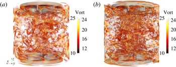
We start by investigating the qualitative behaviour of the flow at high Reynolds numbers. Figure 3 shows snapshots of the vorticity field at
 $R_{e}=10^{4}$
and
 $R_{e}=10^{5}$
characterized by small-scale structures with a clustering near the symmetry axis. The numerous vorticity tubes are characteristic of fully developed turbulence. Elongated vortical structures are attached to the concave side of the impeller blades.
Navier–Stokes simulations in the TM73 VKS2 configuration in the cylinder of radius
 $r=1$
: (a) at
 $R_{e}=10^{4}$
, partial scale for the amplitude of the vorticity field,
 $\Vert \unicode[STIX]{x1D735}\times \boldsymbol{u}\Vert$
(between 10 and 25 for a total scale between 0 and 56) and (b) at
 $R_{e}=10^{5}$
partial scale for the amplitude of the vorticity field,
 $\Vert \unicode[STIX]{x1D735}\times \boldsymbol{u}\Vert$
(between 10 and 25 for a total scale between 0 and 99). The impellers are represented in light grey.

Navier–Stokes simulations in the TM73 VKS2 configuration at
 $R_{e}=10^{5}$
. Snapshots of the velocity field in the plane
 $yOz$
(
 $-1\leqslant y\leqslant 1,-1\leqslant z\leqslant 1$
): (a)
 $u_{x}$
(scale between
 $-0.94$
(blue) and
 $0.85$
(red)); (b)
 $u_{y}$
(scale between
 $-0.83$
(blue) and
 $0.77$
(red)); (c)
 $u_{z}$
(scale between
 $-0.66$
(blue) and
 $0.69$
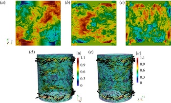
(red). Snapshots of the velocity vector field on the cylindrical surface
 $\{r=0.8\}$
: (d) for
 $-\unicode[STIX]{x03C0}/2\leqslant \unicode[STIX]{x1D703}\leqslant \unicode[STIX]{x03C0}/2$
; (e) for
 $\unicode[STIX]{x03C0}/2\leqslant \unicode[STIX]{x1D703}\leqslant 3\unicode[STIX]{x03C0}/2$
.

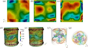
We show in figure 4 one snapshot of the velocity field computed at
 $R_{e}=10^{5}$
. The flow is clearly turbulent as small scales have invaded the entire fluid domain. In the
 $yOz$
plane the velocity components
 $\{u_{x},u_{y}\}$
show ejection motions near the tip of the impellers. Close to the symmetry axis, the
 $u_{z}$
-component shows strong axial motions that are oriented toward the impellers and which are characteristics of the Ekman suction induced by them (see figure 4
a–c). The representation of the velocity vector field on the cylindrical surface
 $\{r=0.8\}$
reveals two counter-rotating zonal flows at the top and bottom of the vessel which are induced by the impellers. We also observe large-scale structures in the equatorial plane where the
 $\{u_{\unicode[STIX]{x1D703}},u_{z}\}$
-components are significantly larger than the radial component
 $u_{r}$
(see figure 4
d,e).
The overall structure is made more visible by inspecting the time average of the velocity field (see figure 5
a–g). We observe two counter-rotating recirculation tori separated by an active azimuthal shear layer localized at the equator. Kinetic energy is injected by the impellers, the flow spirals up or down along the side wall and is driven radially inward at mid-plane. The two resulting inward flows meet at the equator and form a shear layer that dissipates energy. Note that the components of the time-averaged velocity shown in figure 5(a–c) are not fully symmetric with respect to the
 $Oz$
and
 $Oy$
axes due to the presence of the azimuthal Fourier mode
 $m=3$
. The spectra reported in figure 10 show that the azimuthal Fourier mode
 $m=3$
is persistent over a wide range of Reynolds numbers. This energy peak at
 $m=3$
corresponds to three radial co-rotating vortices seen in figure 5(d,e). These cat’s-eye structures are the manifestation of the Kelvin–Helmholtz instability of the equatorial shear layer (Nore et al.
Reference Nore, Tuckerman, Daube and Xin2003). These vortices are localized near the equator and form a complex three-dimensional structure inside the bulk, as evidenced in figure 5(f,g). Similar cat’s-eye vortices have been experimentally observed by Cortet et al. (Reference Cortet, Diribarne, Monchaux, Chiffaudel, Daviaud and Dubrulle2009) at very high Reynolds numbers. It is reported therein that ‘these vortices fluctuate in azimuthal position as well as in amplitude or apparent size’. The fact that these structures are visible in our time average may be due to the Reynolds number not being large enough or the range of the time averaging being too short.
Time-averaged velocity field in Navier–Stokes simulations for the TM73 VKS2 configuration at
 $R_{e}=10^{5}$
. Velocity field in the plane
 $yOz$
(
 $-1\leqslant y\leqslant 1,-1\leqslant z\leqslant 1$
): (a)
 $\overline{u_{x}}$
(scale between
 $-0.75$
(blue) and
 $0.75$
(red)); (b)
 $\overline{u_{y}}$
(scale between
 $-0.34$
(blue) and
 $0.39$
(red)); (c)
 $\overline{u_{z}}$
(scale between
 $-0.37$
(blue) and
 $0.33$
(red)). Velocity vector field on the cylindrical surface
 $\{r=0.8\}$
: (d) for
 $-\unicode[STIX]{x03C0}/2\leqslant \unicode[STIX]{x1D703}\leqslant \unicode[STIX]{x03C0}/2$
; (e) for
 $\unicode[STIX]{x03C0}/2\leqslant \unicode[STIX]{x1D703}\leqslant 3\unicode[STIX]{x03C0}/2$
. Isosurface of 10 % of the velocity magnitude (purple) with streamlines (coloured by velocity magnitude): (f) from a perspective; (g) top view; the cylinder
 $\{r=1\}$
is in light grey.

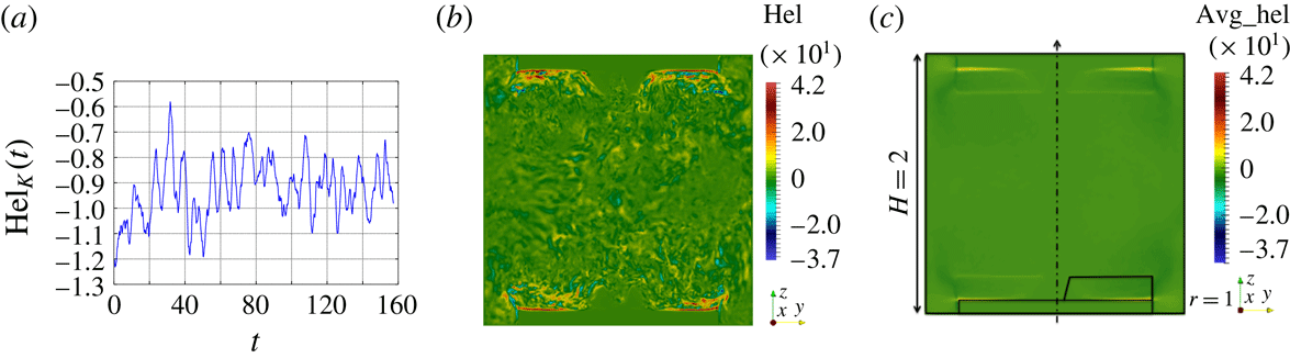
As seen in figure 6(a), the global kinetic helicity
 $\text{Hel}_{K}(t):=\int _{\unicode[STIX]{x1D6FA}}\boldsymbol{u}(\boldsymbol{r},t)\boldsymbol{\cdot }\unicode[STIX]{x1D735}\times \boldsymbol{u}(\boldsymbol{r},t)\,\text{d}\unicode[STIX]{x1D6FA}$
is negative during the entire time of evolution. This is not a surprise since the Ekman suction creates a strong vertical velocity field moving toward each impeller and the product of this velocity field with the angular velocity of the impellers is predominantly negative. However, the spatial distribution of the local helicity
 $\boldsymbol{u}(\boldsymbol{r},t)\boldsymbol{\cdot }\unicode[STIX]{x1D735}\times \boldsymbol{u}(\boldsymbol{r},t)$
is complex and exhibits fine scales (see figure 6
b,c). The maxima are always localized near the impellers whereas the minima are dispersed over the whole fluid domain. This is well illustrated in figure 6(c) where we show the helicity field of the time-averaged velocity. As first numerically evidenced by Ravelet et al. (Reference Ravelet, Dubrulle, Daviaud and Ratié2012), Kreuzahler et al. (Reference Kreuzahler, Schulz, Homann, Ponty and Grauer2014) and seen in figure 3, the positive maxima are associated with the swirling vortices attached to each blade and occupying part of the space between the blades. These vortices are thought to be a key ingredient of the dynamo mechanism (Laguerre et al.
Reference Laguerre, Nore, Ribeiro, Léorat, Guermond and Plunian2008; Gissinger Reference Gissinger2009; Varela et al.
Reference Varela, Brun, Dubrulle and Nore2015).
Navier–Stokes simulations in the TM73 VKS2 configuration at
 $R_{e}=10^{5}$
: (a) time evolution of the total helicity
 $\text{Hel}_{K}(t)$
; (b) snapshot of the helicity in the
 $yOz$
plane at time
 $t=125$
; (c) local helicity of the time-averaged velocity in the
 $yOz$
plane. The dimensions and the contour of the bottom disk and the area swept by the blades are shown in this panel.

3.2 Global quantities
We now make quantitative diagnostics to get a better understanding of the dynamics. Given a finite time series
 $f^{1},\ldots ,f^{q}$
, we define the time average
 $\overline{f}$
as follows:
 $$\begin{eqnarray}\displaystyle \overline{f}:=\displaystyle \frac{1}{q}\mathop{\sum }_{1\leqslant n\leqslant q}f^{n}. & & \displaystyle\end{eqnarray}$$
The first quantities of interest are the kinetic energy
 $E$
, the root mean square velocity and an indicator of the fluctuation level
 $\unicode[STIX]{x1D6FF}$
defined by:
 $$\begin{eqnarray}\displaystyle E(t):=\frac{1}{2}\int _{\unicode[STIX]{x1D6FA}}|\boldsymbol{u}(\boldsymbol{r},t)|^{2}\,\text{d}\unicode[STIX]{x1D6FA},\quad U_{rms}:=\displaystyle \overline{\sqrt{\frac{2E}{|\unicode[STIX]{x1D6FA}|}}},\quad \unicode[STIX]{x1D6FF}(\boldsymbol{u})(t):=\displaystyle \frac{\Vert \boldsymbol{u}\Vert _{L^{2}(\unicode[STIX]{x1D6FA})}^{2}}{\Vert \overline{\boldsymbol{u}}\Vert _{L^{2}(\unicode[STIX]{x1D6FA})}^{2}}. & & \displaystyle\end{eqnarray}$$
We also introduce the poloidal and the toroidal components of the velocity field which we denote by
 $P(\boldsymbol{u})$
and
 $T(\boldsymbol{u})$
, respectively. Using the same notation and convention as in Ravelet (Reference Ravelet2005), we set:
 $$\begin{eqnarray}\displaystyle P(\boldsymbol{u}):=\displaystyle \frac{1}{|\unicode[STIX]{x1D6FA}|}\int _{\unicode[STIX]{x1D6FA}}\sqrt{u_{r,0}^{2}+u_{z,0}^{2}}\,\text{d}\unicode[STIX]{x1D6FA},\quad T(\boldsymbol{u}):=\displaystyle \frac{1}{|\unicode[STIX]{x1D6FA}|}\int _{\unicode[STIX]{x1D6FA}}|u_{\unicode[STIX]{x1D703},0}|\,\text{d}\unicode[STIX]{x1D6FA},\qquad \unicode[STIX]{x1D6E4}(\boldsymbol{u}):=\frac{P(\boldsymbol{u})}{T(\boldsymbol{u})}, & & \displaystyle \nonumber\\ \displaystyle & & \displaystyle\end{eqnarray}$$
where
 $u_{r,0}$
,
 $u_{\unicode[STIX]{x1D703},0}$
and
 $u_{z,0}$
are the radial, azimuthal and vertical components of the Fourier mode
 $m=0$
of the velocity
 $\boldsymbol{u}$
. We finally consider the dimensionless torque
 $K_{p}$
defined by:
 $$\begin{eqnarray}\displaystyle K_{p}=\displaystyle \frac{1}{2}\int _{\unicode[STIX]{x1D6FA}_{solid}}|(\boldsymbol{r}\times \boldsymbol{f}_{s})\boldsymbol{\cdot }\boldsymbol{e}_{z}|\,\text{d}\unicode[STIX]{x1D6FA}, & & \displaystyle\end{eqnarray}$$
where
 $\boldsymbol{f}_{s}$
is the non-dimensional body force that induces the solid rotation of the impellers. Using the notation from (2.2)–(2.4), we deduce from the expression of the discrete momentum balance (2.3) that the torque at time
 $t_{n+1}$
is given by
 $$\begin{eqnarray}\displaystyle K_{p}=\frac{1}{2}\displaystyle \int _{\unicode[STIX]{x1D6FA}}r(1-\unicode[STIX]{x1D712})\text{sign}(z)\frac{1}{2\unicode[STIX]{x1D70F}}(4\boldsymbol{u}^{n}-\boldsymbol{u}^{n-1}-3\boldsymbol{u}_{obs})\boldsymbol{\cdot }\boldsymbol{e}_{\unicode[STIX]{x1D703}}\,\text{d}\unicode[STIX]{x1D6FA}, & & \displaystyle\end{eqnarray}$$
with
 $\text{sign}(z)$
equal to
 $1$
if
 $z>0$
and
 $-1$
otherwise.
We have reported in table 2 the quantities
 $\overline{E}$
,
 $\overline{\unicode[STIX]{x1D6FF}(\boldsymbol{u})}$
,
 $\overline{P(\boldsymbol{u})}$
,
 $\overline{T(\boldsymbol{u})}$
,
 $\overline{\unicode[STIX]{x1D6E4}(\boldsymbol{u})}$
,
 $U_{rms}$
and
 $\overline{K_{p}}$
for all the runs we have done with
 $R_{e}\in \{2\times 10^{2},5\times 10^{2},10^{3},1.5\times 10^{3},2.5\times 10^{3},5\times 10^{3},10^{4},10^{5}\}$
. With the exception of
 $\overline{K_{p}}$
and
 $\overline{\unicode[STIX]{x1D6FF}(\boldsymbol{u})}$
, all the quantities increase with
 $R_{e}$
. In particular the ratio
 $\overline{\unicode[STIX]{x1D6E4}}$
increases with
 $R_{e}$
and reaches the value
 $0.57$
at
 $R_{e}=10^{5}$
. Using TM73 impellers, Ravelet et al. (Reference Ravelet, Chiffaudel, Daviaud and Léorat2005) estimated from measurements in the bulk region
 $0\leqslant r/R_{cyl}\leqslant 1$
,
 $-0.7\leqslant z/R_{cyl}\leqslant 0.7$
that
 $\overline{\unicode[STIX]{x1D6E4}}\approx 0.8$
at
 $R_{e}=10^{5}$
. The ratio
 $\overline{\unicode[STIX]{x1D6E4}}$
is expected to play a major role in the generation of a magnetic field in kinematic dynamo models using time- and azimuth-averaged velocity fields; in particular, values around 0.7 are thought to be near optimal (see figure 5 of Ravelet et al. (Reference Ravelet, Chiffaudel, Daviaud and Léorat2005)) for generating magnetic fields mainly supported by the Fourier mode
 $m=1$
and resembling that of the kinematic dynamo discussed in § 5.1. The values of
 $\overline{\unicode[STIX]{x1D6E4}}$
reported in table 2 are significantly different from those reported in Ravelet et al. (Reference Ravelet, Chiffaudel, Daviaud and Léorat2005). One possible origin for these differences is that we compute
 $\overline{\unicode[STIX]{x1D6E4}}$
whereas it is the quantity
 $P(\overline{\boldsymbol{u}})/T(\overline{\boldsymbol{u}})$
that is estimated in Ravelet et al. (Reference Ravelet, Chiffaudel, Daviaud and Léorat2005) using
 $11\times 17$
laser Doppler velocimetry measurements. Notice finally that the LES results at
 $R_{e}=2.5\times 10^{3}$
are very close to the DNS results at
 $R_{e}=2.5\times 10^{3}$
thereby confirming that, as expected, the entropy viscosity (2.11) vanishes when the flow is well resolved.
Time-averaged
 $\overline{K_{p}}$
versus
 $R_{e}$
in log–linear showing a local maximum around
 $R_{e}=2.5\times 10^{3}$
.

Global quantities as defined in the text for hydrodynamic computations in the TM73 set-up.

Upon inspection of figure 7, where we have reported the time-averaged torque as a function of the Reynolds number, we observe that
 $\overline{K_{p}}$
has a non-monotonic behaviour with respect to
 $R_{e}$
. We also observe that
 $\overline{K_{p}}$
seems to be converging to a non-zero asymptotic limit when
 $R_{e}\rightarrow \infty$
. Note that
 $\overline{\unicode[STIX]{x1D6FF}(\boldsymbol{u})}$
has the same behaviour. The behaviour of
 $\overline{K_{p}}$
and
 $\overline{\unicode[STIX]{x1D6FF}(\boldsymbol{u})}$
is coherent with the theoretical arguments and the experimental observations from Cortet et al. (Reference Cortet, Diribarne, Monchaux, Chiffaudel, Daviaud and Dubrulle2009).
In conclusion, even though our computations are performed at smaller
 $R_{e}$
than in the experiment, the trend followed by the global quantities compares qualitatively well with the experimental results of Ravelet et al. (Reference Ravelet, Chiffaudel and Daviaud2008).
3.3 Kinetic energy versus Reynolds number
We investigate in this section the behaviour of the kinetic energy as the kinetic Reynolds number increases.
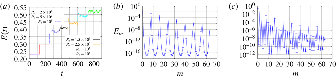
We show in figure 8(a) the time evolution of the kinetic energy
 $E(t)$
for the Reynolds numbers in the range
 $\{2\times 10^{2},5\times 10^{2},10^{3},1.5\times 10^{3},2.5\times 10^{3},10^{4},10^{5}\}$
. There is a unique time series since we have used the final state from the previous run as the initial condition for the next run with a higher Reynolds number. We observe that the flow is steady at
 $R_{e}=2\times 10^{2}$
. It is marginally unsteady at
 $R_{e}=5\times 10^{2}$
, and increasing further
 $R_{e}$
leads to a turbulent regime. The time-averaged kinetic energy
 $\overline{E}$
increases with
 $R_{e}$
as reported in table 2.
(a) Time evolution of the total kinetic energy
 $E(t)$
versus
 $R_{e}$
. Modal kinetic energy
 $E_{m}$
as a function of the azimuthal Fourier mode: (b)
 $R_{e}=2\times 10^{2}$
; (c)
 $R_{e}=5\times 10^{2}$
.

Letting
 $\hat{\boldsymbol{u}}(r,m,z,t)$
be the
 $m$
th complex Fourier component of the velocity field
 $\boldsymbol{u}(r,\unicode[STIX]{x1D703},z,t)$
, we define the kinetic energy of the
 $m$
th Fourier mode by
 $$\begin{eqnarray}\displaystyle E_{m}=\int _{\unicode[STIX]{x1D6FA}_{fluid}^{2D}}\unicode[STIX]{x03C0}|\hat{\boldsymbol{u}}(r,m,z,t)|^{2}r\,\text{d}r\,\text{d}z. & & \displaystyle\end{eqnarray}$$
Figure 8(b,c) shows
 $E_{m}$
as a function of
 $m$
for
 $m\in \{0,\ldots ,63\}$
. The maximum at
 $m=0$
corresponds to the large-scale forcing induced by the rotating disk. The maximum at
 $m=8$
and the maxima at the corresponding harmonics are induced by the eight rotating blades. As expected, only the Fourier mode
 $m=0$
and the mode
 $m=8$
together with its harmonics are populated at
 $R_{e}=2\times 10^{2}$
. This scenario changes when the Reynolds number is slightly increased since all the even Fourier modes are active at
 $R_{e}=5\times 10^{2}$
.
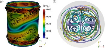
Navier–Stokes simulations in the TM73 VKS2 configuration at
 $R_{e}=5\times 10^{2}$
: (a) snapshot of the velocity vector field on a cylindrical surface at
 $r=0.8$
for
 $-\unicode[STIX]{x03C0}/2\leqslant \unicode[STIX]{x1D703}\leqslant \unicode[STIX]{x03C0}/2$
; (b) isosurface of 6 % of the maximum velocity magnitude (purple) with streamlines (coloured by velocity magnitude) from a top view; the cylinder
 $\{r=1\}$
is in light grey.

At
 $R_{e}=5\times 10^{2}$
the flow is dominated by the Fourier modes
 $m=0$
and
 $m=2$
as illustrated in figure 9. Figure 9(a) shows that the azimuthal shear layer near the equator acquires a wavy structure with two co-rotating radial vortices. This phenomenon has also been observed in Ravelet et al. (Reference Ravelet, Chiffaudel and Daviaud2008). The dominance of the Fourier mode
 $m=2$
and its harmonics is clearly seen when inspecting the velocity streamlines in figure 9(b). The spectrum in figure 8(b) shows that all the even modes are activated by nonlinearity.
As illustrated in figure 10, as
 $R_{e}$
increases further, the axisymmetric mode
 $m=0$
and the Fourier mode
 $m=8$
together with their harmonics are still energetic, but the dynamics becomes richer as the mode
 $m=3$
starts to be active and eventually becomes the second largest after the axisymmetric mode (see figure 10
a). This
 $m=3$
structure (see figure 5) has been visualized in the experiment at very high Reynolds numbers as reported in Cortet et al. (Reference Cortet, Diribarne, Monchaux, Chiffaudel, Daviaud and Dubrulle2009). The structure consists of three radial co-rotating vortices located nearby the equatorial shear layer. The Fourier modes
 $m\in \{0,3,8\}$
and their harmonics are activated by nonlinearity as
 $R_{e}$
grows and eventually the spectrum adopts the
 $m^{-5/3}$
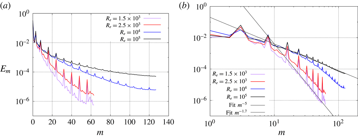
scaling at very high Reynolds number (see figure 10). The quantity
 $E_{m}$
decreases like a negative power of
 $m$
when
 $m$
is large. For instance
 $E_{m}\sim m^{-5}$
for
 $R_{e}=1.5\times 10^{3}$
and
 $E_{m}\sim m^{-1.7}$
for
 $R_{e}=10^{5}$
. The scaling
 $E_{m}\sim m^{-1.7}$
at
 $R_{e}=10^{5}$
is close to
 $m^{-5/3}$
and thereby reminiscent of the Kolmogorov 1941 turbulent scaling for a one-dimensional kinetic energy spectrum (Frisch Reference Frisch1995).
Let us finish this section by noting that a bifurcation similar to the one discussed above, from even modes to odd modes, has been observed and reported in Herbert et al. (Reference Herbert, Cortet, Daviaud and Dubrulle2014) at
 $R_{e}=700$
on a configuration where the impellers are equipped with 16 blades instead of eight and the curvature of the blades is higher. Although the use of planar stereo particle velocimetry made the discrimination between odd modes like
 $m=1$
and
 $m=3$
uneasy, the bifurcation was attributed to a
 $(m=1)$
bifurcation. In this reference the authors have shown that increasing
 $R_{e}$
from
 $10^{2}$
to
 $10^{6}$
leads to non-axisymmetric modulations of the axisymmetric (laminar or time-averaged) flow with successive azimuthal changes in parity (even–odd–even–odd).
Spectra of the kinetic energy
 $E_{m}$
as a function of the azimuthal mode at final time for
 $R_{e}=1.5\times 10^{3},2.5\times 10^{3},10^{4},10^{5}$
: (a) in linear–log scale, (b) in log–log scale with a fit in
 $m^{-5}$
and in
 $m^{-1.7}$
for guiding the eye.

4 MHD results
In this section we solve the full MHD system (2.1a
)–(2.1d
) using as initial velocity field a snapshot computed during the Navier–Stokes runs at the different
 $R_{e}$
. The snapshots are selected at the end of each Navier–Stokes run when the flow is at saturation. The magnetic field
 $\boldsymbol{H}=\boldsymbol{B}/\unicode[STIX]{x1D707}_{0}\unicode[STIX]{x1D707}_{r}$
is initialized to a very small value which we call the seed. Unless specified otherwise, the seed is
 $\boldsymbol{H}_{0}=10^{-6}(\boldsymbol{e}_{z}+\boldsymbol{e}_{x})$
. We also add a random noise of amplitude
 $5\times 10^{-7}$
on all the Fourier modes
 $m\geqslant 1$
of
 $\boldsymbol{H}_{0}$
to arrive at saturation faster. We first explain how we determine the threshold for dynamo action on an illustrative case. Next we study the influence of the relative magnetic permeability of the impellers and the boundary conditions imposed on the outer boundaries of the domain
 $\unicode[STIX]{x1D6FA}\cup \unicode[STIX]{x1D6FA}_{out}$
. We then fix the relative magnetic permeability of the impellers and use the pseudo-vacuum boundary conditions to investigate the variation of the critical magnetic Reynolds number with
 $R_{e}$
.
4.1 Summary of our previous results
We have shown in Nore et al. (Reference Nore, Castanon Quiroz, Cappanera and Guermond2016) that two distinct dynamo families compete at small Reynolds numbers (typically for
 $R_{e}<700$
) and that these two families merge at larger kinetic Reynolds numbers. In the first family, the magnetic field is essentially supported on the even Fourier modes, whereas in the second family the magnetic field is essentially supported on the odd modes; these are called the 0-family and the 1-family in Nore et al. (Reference Nore, Castanon Quiroz, Cappanera and Guermond2016), respectively. In the entire section we focus on
 $R_{e}\geqslant 1.5\times 10^{3}$
; hence all the Fourier modes of the magnetic field are coupled and vary in time with the same (growth or decay) rate in the linear dynamo regime.
4.2 Dynamo threshold and saturation
In this section we fix
 $R_{e}=10^{4}$
and explain how we estimate the dynamo threshold with
 $\unicode[STIX]{x1D707}_{r}^{imp}=50$
and the pseudo-vacuum boundary condition. We are going to use the same methodology for all the other cases. The onset of dynamo action is monitored by recording the time evolution of the magnetic energy in the conducting domain,
 $M(t)=1/2\int _{\unicode[STIX]{x1D6FA}\cup \unicode[STIX]{x1D6FA}_{out}}\boldsymbol{H}(\boldsymbol{r},t)\boldsymbol{\cdot }\boldsymbol{B}(\boldsymbol{r},t)\,\text{d}\boldsymbol{r}=1/2\int _{\unicode[STIX]{x1D6FA}\cup \unicode[STIX]{x1D6FA}_{out}}\unicode[STIX]{x1D707}_{0}\unicode[STIX]{x1D707}_{r}|\boldsymbol{H}(\boldsymbol{r},t)|^{2}\,\text{d}\boldsymbol{r}$
, and the modal energies
 $M_{m}(t)=\int _{\unicode[STIX]{x1D6FA}^{2D}\cup \unicode[STIX]{x1D6FA}_{out}^{2D}}\unicode[STIX]{x03C0}|\hat{\boldsymbol{H}}(r,m,z,t)|^{2}r\,\text{d}r\,\text{d}z$
. Linear dynamo action occurs when
 $M_{m}(t)$
increases exponentially in time (non-oscillating dynamo here) and nonlinear dynamo action takes place when
 $M(t)$
saturates. Various MHD runs are performed with different values of the magnetic Reynolds number
 $R_{m}$
. The threshold for dynamo action is obtained by interpolation on the growth rate between the largest magnetic Reynolds number with a negative growth rate and the smallest magnetic Reynolds number with a positive growth rate. The interpolation is done once the bracketing interval of the threshold is small enough to yield a 5–10 % error estimate. All the thresholds reported in tables 3 and 4 are accompanied with the corresponding uncertainty.
Magnetic thresholds
 $R_{m}^{c}$
for
 $R_{e}=1.5\times 10^{3}$
. ‘
 $\boldsymbol{H}\times \boldsymbol{n}=\mathbf{0}$
’ means pseudo-vacuum boundary condition and ‘vacuum’ means that a larger integration domain with a non-conducting domain around the outer cylinder is used.

Magnetic thresholds
 $R_{m}^{c}$
and critical magnetic Prandtl numbers
 $P_{m}^{c}$
for
 $\unicode[STIX]{x1D707}_{r}^{imp}=50$
versus fluid Reynolds number
 $R_{e}$
. Asterisks represent values from Nore et al. (Reference Nore, Castanon Quiroz, Cappanera and Guermond2016).

4.2.1 Linear regime
At
 $R_{e}=10^{4}$
the velocity field is dominated by the Fourier modes
 $m=0$
and
 $m=3$
as shown in figure 10. Since the coupling term
 $\unicode[STIX]{x1D735}\times (\boldsymbol{u}\times \boldsymbol{B})$
generates even magnetic modes from odd magnetic seeds (for example, the interaction of the seed magnetic mode
 $m=1$
with the velocity mode
 $m=3$
activates the magnetic modes
 $m=2$
and
 $m=4$
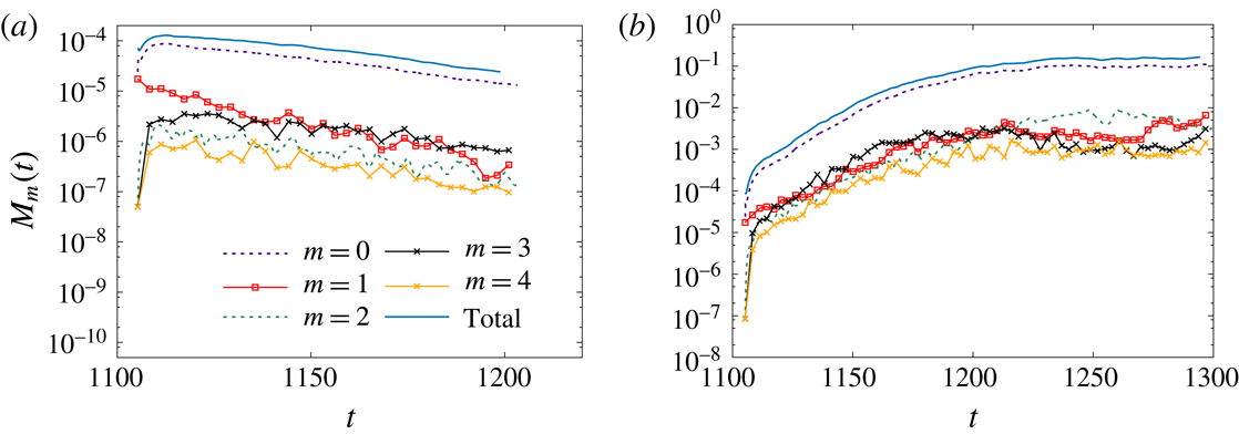
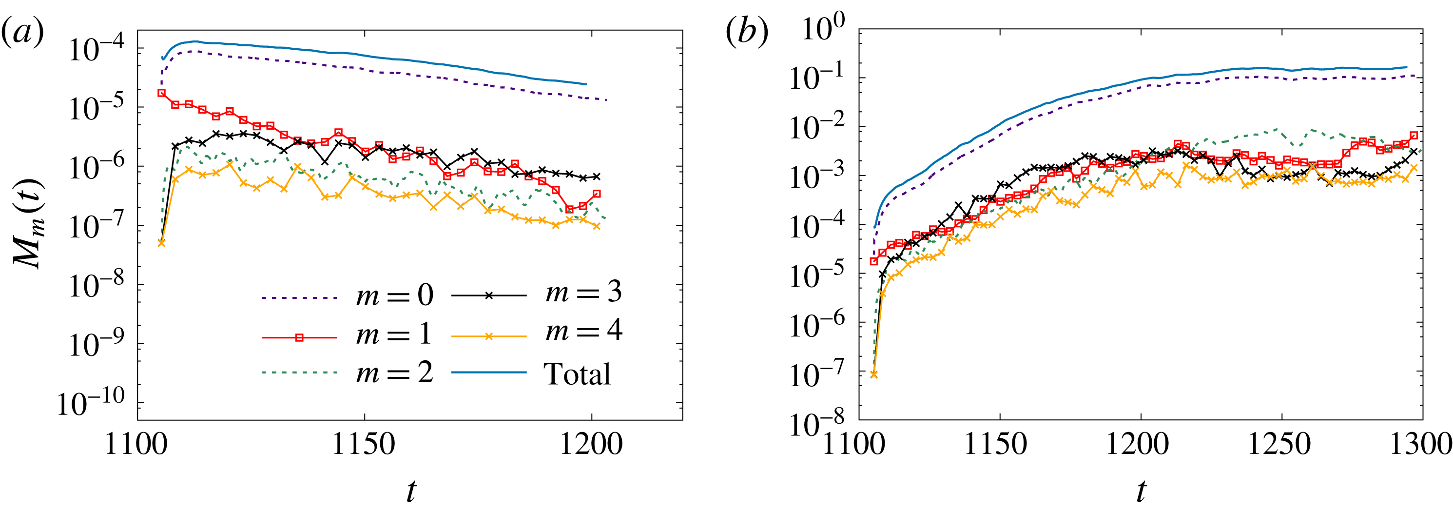
, etc.) and odd magnetic modes from even magnetic seeds, all the Fourier modes of the magnetic field have the same decay or growth rate as reported in figure 11 for
 $R_{m}=50$
and
 $R_{m}=150$
. After estimating the decay rate at
 $R_{m}=50$
and the growth rate at
 $R_{m}=150$
, linear interpolation shows that the threshold in the considered conditions is
 $R_{m}^{c}=75\pm 5$
. All the thresholds on
 $R_{m}$
for dynamo action with
 $\unicode[STIX]{x1D707}_{r}^{imp}=50$
, the pseudo-vacuum boundary condition and
 $R_{e}\in \{2\times 10^{2},5\times 10^{2},10^{3},1.5\times 10^{3},2.5\times 10^{3},5\times 10^{3},10^{4},10^{5}\}$
are reported in table 4.
We show in figure 12 the distribution of the modal energies
 $E_{m}$
and
 $M_{m}$
at two different times for
 $R_{m}=150$
. Note that there is dynamo action at this magnetic Reynolds number. The graphs in figure 12(a) have been done during the linear growth of the magnetic field. Those in figure 12(b) have been obtained at saturation. Note that the spectrum of the magnetic energy during the linear growth resembles that of the kinetic energy; the Fourier modes
 $m\in \{0,3\}$
and the mode
 $m=8$
with its harmonics are dominant.
Time evolution of the total and modal magnetic energies
 $M_{m}(t)$
at
 $R_{e}=10^{4}$
with
 $\unicode[STIX]{x1D707}_{r}^{imp}=50$
for
 $m\in \{0,\ldots ,4\}$
: (a)
 $R_{m}=50$
; (b)
 $R_{m}=150$
.
4.2.2 Nonlinear regime
At
 $R_{m}=150$
we have
 $R_{m}\approx 2\times 75=2R_{m}^{c}$
; hence the simulation done at
 $R_{m}=150$
is far from the threshold, and the Lorentz force is therefore strong enough to retroact on the velocity field in the saturated phase. Figure 12(b) shows that the small azimuthal modes (
 $m\in \{0,\ldots ,4\}$
) of the velocity field and the magnetic field are indeed in competition at saturation (
 $t=1300$
); this can be seen also in figure 11(b) in the time interval
 $t\in [1210,1300]$
. The dominant Fourier modes of the velocity in the saturated regime are now
 $m\in \{0,1,2\}$
as seen in figure 13(a). The kinetic energy decreases while the magnetic energy increases during the time interval
 $t\in [1100,1240]$
as shown in figure 13(b); at
 $t=1250$
both quantities have reached asymptotic values about which they fluctuate. The retroaction of the Lorentz force makes the torque decrease by 40 %; hence, quite surprisingly, driving the flow with a saturated dynamo requires less mechanical power than driving the hydrodynamic base flow (see figure 13
c).
Spectra of the kinetic
 $E_{m}$
and magnetic
 $M_{m}$
energies as a function of the azimuthal mode for
 $R_{e}=10^{4}$
and
 $R_{m}=150$
: (a) in the linear phase at
 $t=1142$
; (b) in the saturation regime at
 $t=1300$
.

Time evolution of (a) the modal kinetic energies
 $E_{m}(t)$
for
 $m\in \{0,\ldots ,4\}$
and for
 $R_{m}=150$
,
 $R_{e}=10^{4}$
and
 $\unicode[STIX]{x1D707}_{r}^{imp}=50$
, (b) the kinetic and magnetic energies and (c) the total torque.

While the retroaction of the Lorentz force on the velocity field in turbulent flows has been studied in various experiments involving applied magnetic fields (see e.g. Sisan, Shew & Lathrop Reference Sisan, Shew and Lathrop2003; Miralles, Plihon & Pinton Reference Miralles, Plihon and Pinton2015), very little is known in this respect when dynamo action occurs. In the Riga experiment, an increase of approximately 10 % of the power consumption has been measured at saturation, and a modification of the swirling profile together with a deceleration of the axial motion has been observed (Gailitis et al. Reference Gailitis, Lielausis, Platacis, Gerbeth and Stefani2003). In the Karlsruhe experiment, a slow down of the axial flow has been recorded in the nonlinear regime (Müller, Stieglitz & Horanyi Reference Müller, Stieglitz and Horanyi2004). In the VKS2 experiment, the modification of the flow in the saturation regime has been too weak to be measured. Note that the range of magnetic Reynolds numbers that can be explored experimentally is limited by the mechanical power that is available; in the above three experiments dynamo action has been investigated only in a small neighbourhood beyond the threshold.
Although very interesting, the study of the nonlinear regime over a large range of parameters is numerically expensive and therefore postponed for future work.
4.3 Impact of the magnetic permeability and boundary conditions on the threshold
We focus in this section on the influence of various parameters on the threshold and we investigate the structure of the growing magnetic field.
4.3.1 Influence of the magnetic permeability
In this section we work with the pseudo-vacuum boundary condition enforced at the outer boundary of the domain
 $\unicode[STIX]{x1D6FA}\cup \unicode[STIX]{x1D6FA}_{out}$
; this boundary condition corresponds to setting
 $\boldsymbol{H}\times \boldsymbol{n}=\mathbf{0}$
, and it is also called perfect ferromagnetic boundary condition in the literature. We also fix the Reynolds number to
 $R_{e}=1.5\times 10^{3}$
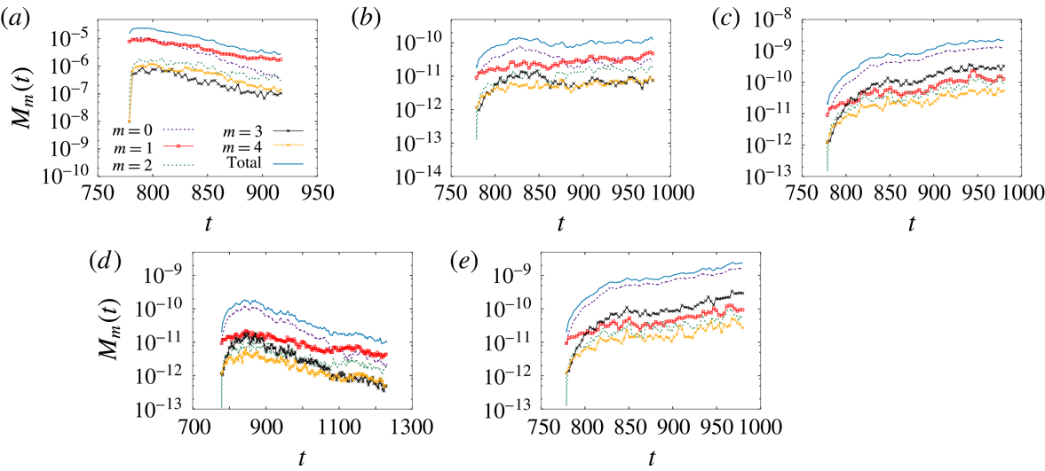
. Figure 14(a–e) shows the time evolution of
 $M_{m}(t)$
for the azimuthal modes
 $m\in \{0,\ldots ,4\}$
for
 $\unicode[STIX]{x1D707}_{r}^{imp}=1$
and
 $\unicode[STIX]{x1D707}_{r}^{imp}=5$
. The computations reported in figure 14(a) have been done with
 $\boldsymbol{H}_{0}=10^{-3}(\boldsymbol{e}_{z}+\boldsymbol{e}_{x})$
plus a random noise of amplitude
 $5\times 10^{-5}$
on all the Fourier modes
 $m\geqslant 1$
of
 $\boldsymbol{H}_{0}$
as in Nore et al. (Reference Nore, Castanon Quiroz, Cappanera and Guermond2016). But since it turned out that this type of perturbation was a bit too large to yield a very accurate estimate of the threshold over reasonable integration times, the other of the computations have been done with
 $\boldsymbol{H}_{0}=10^{-6}(\boldsymbol{e}_{z}+\boldsymbol{e}_{x})$
plus a random noise of amplitude
 $5\times 10^{-7}$
.
When
 $\unicode[STIX]{x1D707}_{r}^{imp}=1$
and near criticality, the behaviour of the magnetic field shows a competition between the modes
 $m=0$
and
 $m=1$
(
 $R_{m}=100,200$
in figures 14
a,b). Well above the threshold, say at
 $R_{m}=300$
and beyond, we recover the same dynamics as that obtained when
 $\unicode[STIX]{x1D707}_{r}^{imp}$
is larger; that is, the axisymmetric magnetic field is dominant and it is preferentially coupled to the mode
 $m=3$
through the velocity field. The threshold for
 $\unicode[STIX]{x1D707}_{r}^{imp}=1$
is estimated to be
 $R_{m}^{c}=190\pm 10$
. The threshold for
 $\unicode[STIX]{x1D707}_{r}^{imp}=5$
is estimated to be
 $R_{m}^{c}=170\pm 5$
. This value is slightly higher than the value
 $R_{m}^{c}\approx 130$
reported in Nore et al. (Reference Nore, Castanon Quiroz, Cappanera and Guermond2016). The likely origin of the discrepancy is that, in order to save CPU time and to reach saturation faster, the initial seed for the magnetic field that was used in Nore et al. (Reference Nore, Castanon Quiroz, Cappanera and Guermond2016) was chosen to be larger than the one presently used, and the integration time was shorter. We believe that the present estimation of
 $R_{m}^{c}$
is probably more accurate. It seems finally that for small values of
 $\unicode[STIX]{x1D707}_{r}^{imp}$
, typically
 $\unicode[STIX]{x1D707}_{r}^{imp}\leqslant 5$
, the dynamics involves interactions between Fourier modes, i.e. the unstable eigenvector is not a pure Fourier mode in azimuth, whereas the axisymmetric mode dominates when
 $\unicode[STIX]{x1D707}_{r}$
is large. Hence when
 $\unicode[STIX]{x1D707}_{r}$
is large we obtain clearer decay or growth rate, and, consequently, it is easier to estimate the threshold. The largest value of the relative permeability used in the present paper is
 $\unicode[STIX]{x1D707}_{r}^{imp}=50$
.
Time evolution of the total and modal magnetic energies
 $M_{m}(t)$
at
 $R_{e}=1.5\times 10^{3}$
with pseudo-vacuum boundary condition for
 $m\in \{0,\ldots ,4\}$
: (a–c)
 $R_{m}\in \{100,200,300\}$
and
 $\unicode[STIX]{x1D707}_{r}^{imp}=1$
; (d,e)
 $R_{m}\in \{150,200\}$
and
 $\unicode[STIX]{x1D707}_{r}^{imp}=5$
.

4.3.2 Influence of the boundary conditions
To test the influence of boundary conditions, we now enlarge the computational domain by adding an insulator around the VKS2 container (air or vacuum). The outer boundary of the computational domain is now a sphere centred at the origin and of radius 10. The magnetic field in the insulator is represented as the gradient of a scalar potential as in Guermond et al. (Reference Guermond, Laguerre, Léorat and Nore2009) and this potential is enforced to be zero on the outer sphere. This configuration is a better representation of the actual experiment than that with the pseudo-vacuum boundary condition, but it is computationally more expensive.
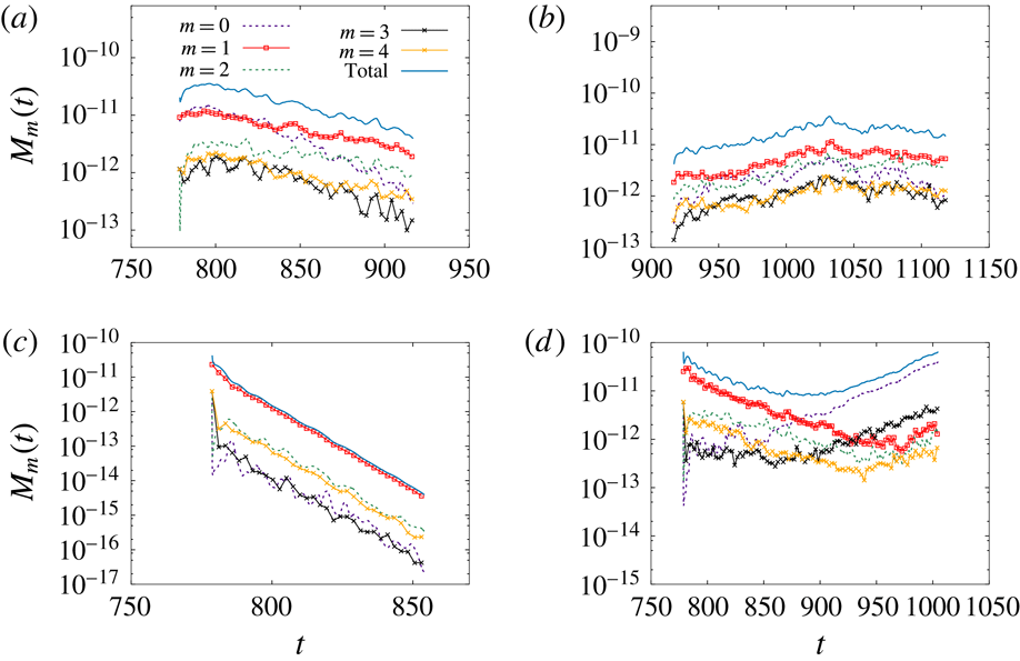
We show in figure 15 the time evolution of the magnetic energy at
 $R_{e}=1.5\times 10^{3}$
for the Fourier modes
 $m\in \{0,\ldots ,4\}$
with
 $\unicode[STIX]{x1D707}_{r}^{imp}=1$
(figure 15
a,b) and with
 $\unicode[STIX]{x1D707}_{r}^{imp}=50$
(figure 15
c,d). These computations have been done with the vacuum boundary condition. The seed for the magnetic field is
 $\boldsymbol{H}_{0}=10^{-6}\boldsymbol{e}_{x}$
plus a random noise of amplitude
 $5\times 10^{-7}$
. We removed the axial component of the seed to demonstrate unequivocally that the axial component of the axisymmetric mode grows above the dynamo threshold. Other computations (not shown here) done with the standard seed described at the beginning of § 4 give very similar results.
Time evolution of the total and modal magnetic energies
 $M_{m}(t)$
at
 $R_{e}=1.5\times 10^{3}$
with vacuum boundary condition for
 $m\in \{0,\ldots ,4\}$
: (a,b)
 $R_{m}\in \{150,300\}$
and
 $\unicode[STIX]{x1D707}_{r}^{imp}=1$
; (c,d)
 $R_{m}\in \{50,150\}$
and
 $\unicode[STIX]{x1D707}_{r}^{imp}=50$
.

For
 $\unicode[STIX]{x1D707}_{r}^{imp}=1$
, the two Fourier modes
 $m=1$
and
 $m=2$
compete below and above the threshold. The threshold in this case is larger than when the pseudo-vacuum boundary condition is imposed. We obtain here
 $R_{m}^{c}=310\pm 30$
whereas we had
 $R_{m}^{c}=190\pm 10$
with the pseudo-vacuum boundary condition. The increase is approximately 60 %. The magnetic field is mainly supported on the Fourier modes
 $m=1$
and
 $m=2$
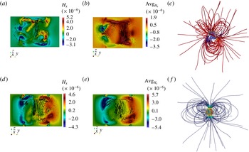
with a complex three-dimensional structure as shown on figure 16(a–c).
For
 $\unicode[STIX]{x1D707}_{r}^{imp}=50$
the threshold is estimated to be at
 $R_{m}^{c}=130\pm 10$
(figure 15
c,d). Inspection of figure 15(d) reveals that at
 $R_{m}=150$
the Fourier mode
 $m=1$
decreases in time, while the modes
 $m=0$
and
 $m=3$
increase and transfer energy to the other modes by nonlinear interactions for
 $t\geqslant 850$
. This scenario is reminiscent of the crossing of the modes
 $m=1$
and
 $m=0$
discussed in Boisson & Dubrulle (Reference Boisson and Dubrulle2011). The present simulations show that the magnetic field is not purely axisymmetric since a significant portion of the magnetic energy is carried by the Fourier mode
 $m=3$
. We will examine the relative importance of the non-axisymmetric modes in § 4.5. As shown in figure 16(d–f) the growing magnetic field is mainly an axial dipole with an azimuthal component approximately even in
 $z$
. The structure of a snapshot of the magnetic field (figure 16
d) and the structure of the time-averaged magnetic field (figure 16
e) are similar to those obtained with the pseudo-vacuum boundary condition (see figure 18
a,b). This structure is also compatible with the measurements of the magnetic field made at saturation during the dynamo regime obtained in the VKS2 configuration with soft iron impellers and a copper container (see figure 6b in Boisson et al. (Reference Boisson, Aumaitre, Bonnefoy, Bourgoin, Daviaud, Dubrulle, Odier, Pinton, Plihon and Verhille2012)).
When one compares the estimations of the threshold using
 $\unicode[STIX]{x1D707}_{r}^{imp}=50$
and the pseudo-vacuum boundary condition,
 $R_{m}^{c}=90\pm 5$
, with that obtained with
 $\unicode[STIX]{x1D707}_{r}^{imp}=50$
and the vacuum boundary condition,
 $R_{m}^{c}=130\pm 10$
, we observe a 40 % increase. This dependence of the dynamo threshold on the boundary condition is compatible with the observation made in Guermond et al. (Reference Guermond, Léorat, Luddens, Nore and Ribeiro2011a
), Gissinger et al. (Reference Gissinger, Iskakov, Fauve and Dormy2008) using kinematic dynamo simulations. It is shown in these references that the perfect ferromagnetic boundary condition decreases the dynamo threshold, the minimum being achieved when this boundary condition is enforced over the entire boundary of the container. This is explained by a screening mechanism of the walls. The present full MHD simulations show the same trend.
Magnetic field from full MHD simulations in the TM73 VKS2 configuration at
 $R_{e}=1.5\times 10^{3}$
with vacuum boundary condition: (a,b)
 $R_{m}=300$
,
 $\unicode[STIX]{x1D707}_{r}^{imp}=1$
, snapshot and time-averaged magnetic field in
 $\unicode[STIX]{x1D6FA}_{c}$
; (c)
 $R_{m}=300$
,
 $\unicode[STIX]{x1D707}_{r}^{imp}=1$
, magnetic field lines in the whole domain; (d,e)
 $R_{m}=150$
,
 $\unicode[STIX]{x1D707}_{r}^{imp}=50$
, snapshot and time-averaged magnetic field in
 $\unicode[STIX]{x1D6FA}_{c}$
; (f)
 $R_{m}=150$
,
 $\unicode[STIX]{x1D707}_{r}^{imp}=50$
, magnetic field lines in the whole domain. In (a,b,d,e) arrows represent in-plane
 $\{H_{y},H_{z}\}$
vectors and colour represents the out-of-plane component
 $H_{x}$
.

The data collected in table 3 lead to the conclusion that using the ferromagnetic boundary condition on the external boundary of the container and using ferromagnetic material for the impeller with a large value of the magnetic permeability decreases the dynamo threshold and enhances the axisymmetric component of the magnetic field produced by the dynamo effect.
A similar dominant axisymmetric magnetic field is also observed at
 $R_{e}=2025$
and
 $P_{m}=1/3$
for
 $\unicode[STIX]{x1D707}_{r}^{imp}\geqslant 12$
in Kreuzahler et al. (Reference Kreuzahler, Ponty, Plihon, Homann and Grauer2017). In this paper, the authors study the dynamo action in the von Kármán sodium experiment for four values of the Reynolds number and three values of the magnetic Reynolds number (up to
 $R_{e}=2025$
and
 $R_{m}=1012.5$
, using the same definitions for these control parameters as in the present article). There are similarities between the present paper and this recent reference since both works use similar penalty methods and evidence the same dominant axisymmetric dipolar magnetic field when the relative magnetic permeability of the impellers is large enough, as already pointed out by Nore et al. (Reference Nore, Castanon Quiroz, Cappanera and Guermond2016). However there are two key differences between the two papers: (i) we determine thresholds over a wider range of kinetic Reynolds numbers and for larger values of relative magnetic permeability of the impellers; the largest value of the relative magnetic permeability reached in Kreuzahler et al. (Reference Kreuzahler, Ponty, Plihon, Homann and Grauer2017) is 16, whereas we reach
 $\unicode[STIX]{x1D707}_{r}^{imp}=50$
, (this value of the relative magnetic permeability of the soft iron impellers is of the same order as that measured in the experiment, Verhille et al. (Reference Verhille, Plihon, Bourgoin, Odier and Pinton2010)). (ii) The penalty method in Kreuzahler et al. (Reference Kreuzahler, Ponty, Plihon, Homann and Grauer2017) is used for the fluid part only (to confine the flow in a cylinder and to drive it with the impellers); therefore, the magnetic part is only crudely modelled, since the conductivity is assumed to be constant everywhere. This makes comparisons with the present work difficult, as we showed in table 3 that boundary conditions have a large influence on the actual values of the thresholds.
4.4 Threshold at
 $\unicode[STIX]{x1D707}_{r}^{imp}=50$
versus
$R_{e}$


We put ourselves in this section in the most favourable configuration for dynamo action to occur: we enforce the ferromagnetic boundary condition on the external boundary of the container and we use
 $\unicode[STIX]{x1D707}_{r}^{imp}=50$
. We now investigate the evolution of the critical magnetic Reynolds number as a function of the kinetic Reynolds number.
 $R_{m}^{c}$
versus
 $R_{e}$
in log–linear at
 $\unicode[STIX]{x1D707}_{r}^{imp}=50$
.
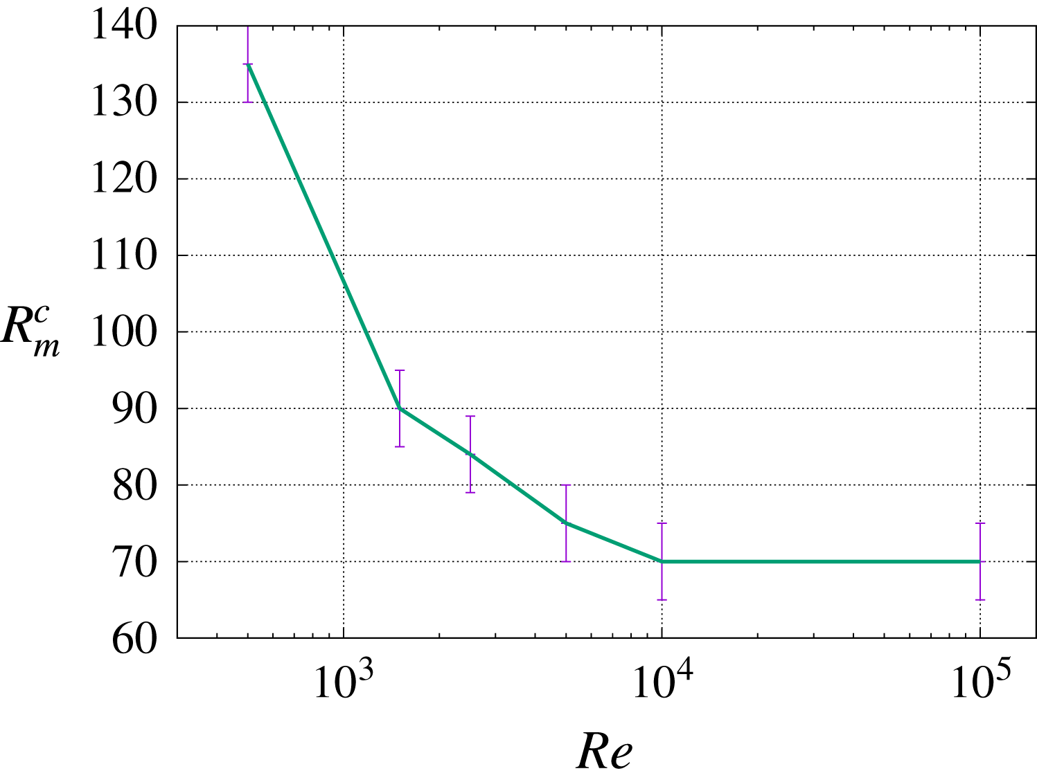
We have reported in figure 17 the estimated value of
 $R_{m}^{c}$
for
 $R_{e}\in \{5\times 10^{2},1.5\times 10^{3},$
 $2.5\times 10^{3},5\times 10^{3},10^{4},10^{5}\}$
. The critical magnetic Reynolds number seems to tend to an asymptotic value
 ${R_{m}^{c}}_{\infty }$
as the kinetic Reynolds number tends to infinity. Since the kinetic Reynolds numbers associated with dynamo action in the VKS2 experiment are in the range
 $6.3\times 10^{6}\leqslant R_{e}\leqslant 8.7\times 10^{6}$
(see § 2.1), figure 17 leads us to conjecture that the critical magnetic Reynolds number in this range is close to
 ${R_{m}^{c}}_{\infty }$
. It is indeed remarkable that the asymptotic value
 ${R_{m}^{c}}_{\infty }\approx 70$
is in the range
 $[52,71]$
where dynamo action has been experimentally observed.
Assuming, as suggested by the results reported in table 3, that going from
 $\unicode[STIX]{x1D707}_{r}^{imp}\approx 50$
to
 $\unicode[STIX]{x1D707}_{r}^{imp}=1$
doubles the threshold for dynamo action (uniformly in
 $R_{e}$
), it is reasonable to expect that the asymptotic limit
 ${R_{m}^{c}}_{\infty }$
for
 $\unicode[STIX]{x1D707}_{r}^{imp}=1$
is approximately
 $70\times 2\approx 140$
. Hence, we conjecture that the threshold on the VKS experiment with impellers made of stainless steel might be
 $R_{m}^{c}\simeq 140$
. The estimate of the threshold obtained experimentally by measurements of the decay time in this configuration (see Miralles et al. (Reference Miralles, Bonnefoy, Bourgoin, Odier, Pinton, Plihon, Verhille, Boisson, Daviaud and Dubrulle2013): run O in figure 6, threshold reported in table 1 and
 $R_{m}$
defined at line 24, page 8) gives
 $R_{m}^{c}\simeq 110$
, which is in reasonable agreement with our conjectured value
 $R_{m}^{c}\simeq 140$
considering that the ferromagnetic walls in run O are closer to the impellers than in our computations.
Magnetic field from full MHD simulations in the TM73 VKS2 configuration in the saturated regime at
 $R_{e}=1.5\times 10^{3}$
,
 $R_{m}=150$
and
 $\unicode[STIX]{x1D707}_{r}^{imp}=50$
, pseudo-vacuum boundary condition: (a,b) arrows represent in-plane
 $\{H_{y},H_{z}\}$
vectors, colour represents the out-of-plane component
 $H_{x}$
, the cylinder axis is in the middle (from Nore et al. (Reference Nore, Castanon Quiroz, Cappanera and Guermond2016)). (c) Magnetic field lines of
 $\overline{\boldsymbol{H}}$
coloured by
 $\overline{H_{z}}$
; (d) isosurface of 50 % of the maximum amplitude of
 $\Vert \overline{\boldsymbol{H}}\Vert$
and cut at
 $z=0$
for
 $\{r\leqslant 1.6\}$
; (e) cut at
 $z=0$
from top view coloured by
 $\overline{H_{z}}$
(the inner cylinder of radius
 $r=1$
is indicated in light grey, the outer radius is 1.6).

4.5 Spatial structure of the magnetic field versus
$R_{e}$

We continue with the pseudo-vacuum boundary conditions and
 $\unicode[STIX]{x1D707}_{r}^{imp}=50$
. Figures 18 and 19 show a snapshot of the magnetic field and the time-averaged magnetic field obtained at saturation in the dynamo regime at
 $R_{e}=1.5\times 10^{3}$
and
 $R_{e}=10^{5}$
, respectively. Although the time-averaged magnetic field at
 $R_{e}=1.5\times 10^{3}$
and at
 $R_{e}=10^{5}$
look similar, we observe on the two snapshots in figures 18(a) and 19(a) that the magnetic field at
 $R_{e}=10^{5}$
exhibits bursts near the impellers, whereas the magnetic field at
 $R_{e}=1.5\times 10^{3}$
is smoother. Notice also that the time-averaged magnetic vector field in the
 $yOz$
plane is not strictly symmetric with respect to the
 $Oz$
axis. The ratio of the magnetic energy supported by the Fourier modes
 $m\geqslant 1$
to the total magnetic energy is approximately 11 % for
 $R_{e}=1.5\times 10^{3}$
,
 $R_{m}=150$
and it is approximately 18 % for
 $R_{e}=10^{5}$
,
 $R_{m}=100$
. This little departure from axisymmetry gives a wavy shape to the magnetic field streamlines as shown in figures 18(c) and 19(c). The dominant non-axisymmetric Fourier mode of the magnetic field is
 $m=3$
as shown in figures 18(d,e) and 19(d,e).
Although the flows at
 $R_{e}=1.5\times 10^{3}$
and
 $R_{e}=10^{5}$
are quite different, the time-averaged magnetic fields produced by dynamo action are very similar: compare figures 18(b) and 19(b). This observation leads us to conjecture that the time-averaged magnetic field might have the same shape for the actual Reynolds number
 $R_{e}\approx 5\times 10^{6}$
. At least the axisymmetric shape in figures 18(b) and 19(b) is similar to the one reconstructed in figure 6(b) in Boisson et al. (Reference Boisson, Aumaitre, Bonnefoy, Bourgoin, Daviaud, Dubrulle, Odier, Pinton, Plihon and Verhille2012). Of course, the scarcity of experimental data (Gaussmeters on a few lines) gives little information on the non-axisymmetric components.
Same as figure 18 with
 $R_{e}=10^{5}$
,
 $R_{m}=100$
and
 $\unicode[STIX]{x1D707}_{r}^{imp}=50$
. The non-dimensional geometric dimensions of the set-up are shown in (b).

5 Simplified models
In this section we investigate whether the mostly axisymmetric structure of the dynamo can be recovered by performing kinematic dynamo computations with flat disks and the time average of the velocity field obtained at
 $R_{e}=10^{5}$
and shown in figure 5. We also take a closer look at the structure of the electrical current that is generated by dynamo action in the full MHD simulations and propose a simple interpretation of the observed dynamo.
5.1 Kinematic dynamo using the time-averaged velocity field at
$R_{e}=10^{5}$

A kinematic dynamo simulation is done by solving only the induction equation (2.1b
) and by using the time-averaged velocity field obtained at
 $R_{e}=10^{5}$
; this field is shown in figure 5. The time-averaged velocity field is not axisymmetric and therefore may sustain an axisymmetric magnetic field since Cowling’s theorem does not apply. We also use flat ferromagnetic disks with
 $\unicode[STIX]{x1D707}_{r}^{imp}=50$
and we impose the boundary condition
 $\boldsymbol{H}\times \boldsymbol{n}=\mathbf{0}$
on the outer wall of the container.
We perform simulations with
 $R_{m}\in [50,200]$
and find that the Fourier modes
 $m\in \{1,2,4\}$
can grow while the modes
 $m\in \{0,3\}$
always decrease. The dynamo threshold is
 $R_{m}^{c}\approx 120\pm 5$
and the growing magnetic field has a strong Fourier component supported on the mode
 $m=1$
. This unstable eigenmode has the shape of an equatorial dipole with two opposite axial structures (see figure 20). This magnetic field is similar to the one obtained in Ravelet et al. (Reference Ravelet, Chiffaudel, Daviaud and Léorat2005), Guermond et al. (Reference Guermond, Léorat, Luddens, Nore and Ribeiro2011a
) using the time- and azimuth-averaged flow measured in a von Kármán experiment done in water. In these references the amplitude of the velocity field has been multiplied by factors in the range
 $[0.6,0.75]$
to test various scenarios and to make the definitions of
 $R_{e}$
adopted in these references coincide. Once we take into account this multiplicative factor (between 0.6 and 0.75), the threshold
 $R_{m}^{c}\approx 120$
that we obtain is in the range of those published in the above references; for instance
 $43/0.75\leqslant R_{m}^{c}\leqslant 180/0.6$
in Ravelet et al. (Reference Ravelet, Chiffaudel, Daviaud and Léorat2005) and
 $40/0.75\leqslant R_{m}^{c}\leqslant 82/0.6$
in Guermond et al. (Reference Guermond, Léorat, Luddens, Nore and Ribeiro2011a
).
The main point of the present discussion is that the kinematic dynamo computation realized with the time-averaged velocity field obtained at
 $R_{e}=10^{5}$
gives a dynamo that is totally different from the one obtained with the full velocity field since it is mainly supported on the Fourier mode
 $m=1$
. Therefore the mainly axisymmetric magnetic field shown in figure 19 cannot be attributed to the time-averaged velocity field only.
Magnetic field from kinematic dynamo simulations using the time-averaged velocity field at
 $R_{e}=10^{5}$
with
 $R_{m}=150$
and
 $\unicode[STIX]{x1D707}_{r}^{imp}=50$
: (a) arrows represent in-plane
 $\{H_{y},H_{z}\}$
vectors, colour represents the out-of-plane component
 $H_{x}$
, the cylinder axis is in the middle; (b) isosurface of the magnetic magnitude (coloured by the
 $H_{z}$
component: red for upward direction and green for downward direction) at 30 % of the maximum with magnetic vector fields.

5.2 Spatial structure of the electric current versus
$R_{e}$

We now focus our attention on the electric current produced by the full MHD dynamo. Figure 21(a,b) shows the electric current associated with the time-averaged magnetic field computed at
 $R_{e}=1.5\times 10^{3}$
with
 $R_{m}=150$
; figure 21(c,d) shows the electric current associated with the time-averaged magnetic field computed at
 $R_{e}=10^{5}$
with
 $R_{m}=100$
. In both cases we use
 $\unicode[STIX]{x1D707}_{r}^{imp}=50$
. The current distribution shows large-scale meridian loops. The current lines close to the axis have the shape of a left-handed helix going downwards; they are mainly radial in the disks (flowing outwards in the bottom disk and inwards in the top disk); they are mainly vertical and flow upwards in the copper wall (
 $j_{z}$
is positive in figure 21(b–d) in the ring
 $\{1.4\leqslant r\leqslant 1.6;z=0\}$
). The current lines also form smaller meridian loops near the blades. The poloidal component of the current (
 $\{j_{r},j_{z}\}$
in the copper wall and near the blades) generates the toroidal
 $H_{\unicode[STIX]{x1D703}}$
field, while the toroidal
 $j_{\unicode[STIX]{x1D703}}$
component of the twisted helical current lines near the axis creates the axial
 $H_{z}$
magnetic field. This organization of the current evokes the disk–dynamo of Bullard (Reference Bullard1955) with two disks (instead of one only). The radial current in the bottom disk is collected in the copper walls, injected in the top disk, and flows from the top disk to the bottom disk in a left-handed helix. The left-hand twist of the current lines in the bulk near the cylinder axis is induced by the flow of liquid sodium. Figure 22(a) shows the current lines coloured by
 $\Vert \boldsymbol{j}\Vert$
. The current amplitude is strong near the axis. A schematic representation of the double-disk Bullard dynamo is shown in figure 22(b).
Electric current field from time-averaged magnetic field,
 $\unicode[STIX]{x1D707}_{r}^{imp}=50$
: (a,b)
 $R_{e}=1.5\times 10^{3}$
,
 $R_{m}=150$
; (c,d)
 $R_{e}=10^{5}$
,
 $R_{m}=100$
; (a,c) streamlines of the current
 $\overline{\boldsymbol{j}}=\unicode[STIX]{x1D735}\times \overline{\boldsymbol{H}}$
coloured by the magnitude of
 $\Vert \overline{\boldsymbol{H}}\Vert$
; (b,d) current streamlines coloured by the magnitude of
 $\Vert \overline{\boldsymbol{H}}\Vert$
and slice at
 $\{z=0\}$
coloured by
 $\overline{j_{z}}$
.

Current distribution: (a) current streamlines coloured by the magnitude of
 $\Vert \overline{\boldsymbol{j}}\Vert$
(in log scale); (b) schematic of the dominant current field lines giving rise to the predominant axisymmetric time-averaged magnetic field of figure 19.

6 Summary and discussion
The main outcomes of the present paper are the following points:
(i) The hydrodynamic computations using the entropy–viscosity-based LES technique give results in agreement with the experimental data at high Reynolds numbers. The global experimental and numerical kinetic quantities behave similarly when
$R_{e}$
increases. The modal spectrum of the kinetic energy is dominated by the azimuthal Fourier modes
$m\in \{0,2\}$
for
$R_{e}<700$
and
$m\in \{0,3\}$
for larger
$R_{e}$
. At
$R_{e}=10^{5}$
, the modal spectrum behaves like
$m^{-5/3}$
when
$m$
is large. In the physical space, the leading Fourier mode
$m=2$
found at
$R_{e}=5\times 10^{2}$
corresponds to the wavy bifurcation reported in Ravelet et al. (Reference Ravelet, Chiffaudel and Daviaud2008). At larger
$R_{e}$
, the Fourier mode
$m=3$
is related to the three radial co-rotating vortices localized near the equatorial shear layer as observed by Cortet et al. (Reference Cortet, Diribarne, Monchaux, Chiffaudel, Daviaud and Dubrulle2009) in a von Kármán experiment using water.(ii) The full MHD computations show that, at fixed
$R_{e}$
, increasing the relative magnetic permeability of the impellers and/or using ferromagnetic material at the outer boundaries of
$\unicode[STIX]{x1D6FA}\cup \unicode[STIX]{x1D6FA}_{out}$
decreases the threshold (using the pseudo-vacuum boundary condition is equivalent to adding a material with infinite permeability at the boundary). The ferromagnetic impellers enhance the axisymmetric magnetic field (Giesecke et al.
Reference Giesecke, Nore, Stefani, Gerbeth, Léorat, Herreman, Luddens and Guermond2012) and ferromagnetic outer walls confine the magnetic field inside the vessel. At fixed
$\unicode[STIX]{x1D707}_{r}$
, increasing the kinetic Reynolds number also reduces the threshold. Moreover, the overall shape of the critical magnetic field averaged in time barely changes between
$R_{e}=1.5\times 10^{3}$
and
$R_{e}=10^{5}$
as shown in figures 18 and 19. This robustness with respect to the kinetic Reynolds number may explain why the magnetic field that we computed is in very good agreement with the mainly axisymmetric magnetic field that has been experimentally observed at much higher Reynolds numbers (compare figures 18
b and 19
b with figure 6b in Boisson et al. (Reference Boisson, Aumaitre, Bonnefoy, Bourgoin, Daviaud, Dubrulle, Odier, Pinton, Plihon and Verhille2012)).(iii) Using ferromagnetic boundary conditions and
$\unicode[STIX]{x1D707}_{r}^{imp}=50$
, we have found that the critical magnetic Reynolds number tends to an asymptotic value
${R_{m}^{c}}_{\infty }\approx 70$
when
$R_{e}$
increases. This value is in the range
$52\leqslant R_{m}^{c}\leqslant 71$
where dynamo action has been observed in the VKS2 set-up (see table I in Miralles et al. (Reference Miralles, Bonnefoy, Bourgoin, Odier, Pinton, Plihon, Verhille, Boisson, Daviaud and Dubrulle2013)). The behaviour of
$R_{m}^{c}$
with respect to
$R_{e}$
that we observed suggests that the small scales of turbulence do not seem to intervene in the dynamo mechanism at high
$R_{e}$
numbers. This behaviour is somewhat at odd with other computations using simplistic forcings like Iskakov et al. (Reference Iskakov, Schekochihin, Cowley, McWilliams and Proctor2007), Ponty et al. (Reference Ponty, Mininni, Pinton, Politano and Pouquet2007), Reuter, Jenko & Forest (Reference Reuter, Jenko and Forest2011), Ponty & Plunian (Reference Ponty and Plunian2011). In all these simulations the critical magnetic Reynolds number has a non-monotonic behaviour with respect to
$R_{e}$
. It first increases with
$R_{e}$
, then either reaches a plateau or decreases after some intermediate value of
$R_{e}$
in the range
$[200,1500]$
. Finally, it is suggested in Ponty & Plunian (Reference Ponty and Plunian2011) that ‘it is the mean flow which plays the most important role in the field generation even though it is 40 % less intense than the fluctuations’. As shown in figure 10, the azimuthal Fourier modes
$m\in \{0,3\}$
of the velocity contain most of the total kinetic energy at all the kinetic Reynolds numbers we have explored (the smallest being
$R_{e}=500$
). For instance these two modes contain about 75 % of the total kinetic energy at
$R_{e}=10^{5}$
. However the kinematic computations of § 5.1 have proved that the mean flow (averaged in time but not in space, therefore with non-axisymmetric features) gives a dynamo with a magnetic field mainly supported by the Fourier mode
$m=1$
as already reported in the literature by us and others using an experimental time- and azimuth-averaged velocity field. Therefore the VKS2 dynamo cannot be attributed to the mean flow.


To conclude, our simulations at high
 $R_{e}$
numbers confirm that the ferromagnetic impellers are crucial to reduce the dynamo threshold and to obtain the predominantly axisymmetric dynamo mode observed in the VKS2 experimental set-up. Looking at figure 22, where a schematic representation of the path followed by the electrical current is shown, the following speculative mechanism comes to mind: Let us imagine a vertical magnetic seed pointing upwards near one rotating impeller; by
 $\unicode[STIX]{x1D6FA}$
-effect, the differential rotation of the impeller generates a toroidal magnetic field nearby the disk. This toroidal field is associated with a radial current (
 $j_{r}\approx -\unicode[STIX]{x2202}_{z}H_{\unicode[STIX]{x1D703}}$
) flowing outward in the bottom impeller and inward in the top one. The current circulates from the bottom impeller to the top one through a large-scale loop inside the copper wall. Near the axis of the vessel the current flows downwards and the current lines are twisted by the flow in a way that regenerates the initial vertical field. This is the Bullard dynamo loop (Bullard Reference Bullard1955) with the
 $\unicode[STIX]{x1D6FA}$
-effect due to the disks and the twisting effect due to the flow.
Acknowledgement
The HPC resources for SFEMaNS were provided by GENCI-IDRIS (grant 2016-0254) in France and by the Texas A&M University Brazos HPC cluster. J.-L.G. acknowledges support from University Paris Sud, the National Science Foundation under grants DMS 1620058, DMS 1619892, the Air Force Office of Scientific Research, USAF, under grant/contract number FA99550-12-0358 and the Army Research Office, under grant number W911NF-15-1-0517. D.C.Q. acknowledges support by the Basque Government through ELKARTEK and the BERC 2014-2017 programmes and by Spanish Ministry of Economy and Competitiveness MINECO: BCAM Severo Ochoa excellence accreditation SEV-2013-0323. L.C. is thankful to Texas A&M University, LIMSI, and CNRS for their financial support. W. Herreman at LIMSI is greatly acknowledged for fruitful discussions and drawing figures 1 and 22(b).