1. Introduction
The process leading to the atomization of a slow liquid stream assisted by a fast air stream is often described using the concept of ‘instability cascade’ (Marmottant & Villermaux Reference Marmottant and Villermaux2004). A first shear instability creates a wave that develops farther downstream, leading to the generation of liquid ligaments that are then stretched and broken into small droplets. This process, called primary atomization, is followed by droplets–droplets and droplets–turbulence interactions, i.e. the secondary atomization, see Lefebvre (Reference Lefebvre1989) for an extensive review.
The primary wave occurring due to the shear instability is created by means of a Kelvin–Helmholtz-like instability. The parallel, or quasi-parallel, nature of the flow close to the injector makes it an idealized framework for linear stability analysis. In the limit of a large gas velocity  $U_g$, the wave frequency
 $f$ scales as (Raynal Reference Raynal1997; Marmottant & Villermaux Reference Marmottant and Villermaux2004)
 \begin{equation} f \sim U_g^{3/2}. \end{equation}
This scaling has been extensively observed in experiments (Ben Rayana Reference Ben Rayana2007; Matas, Marty & Cartellier Reference Matas, Marty and Cartellier2011) and simulations at reduced density ratio (Fuster et al. Reference Fuster, Matas, Marty, Popinet, Hoepffner, Cartellier and Zaleski2013). In Raynal (Reference Raynal1997) and Ben Rayana (Reference Ben Rayana2007), the wave velocity is found to be in very good agreement with (Dimotakis Reference Dimotakis1986)
 \begin{equation} U_D = \frac{\sqrt{\rho_l}U_l + \sqrt{\rho_g}U_g}{\sqrt{\rho_l} + \sqrt{\rho_g}}, \end{equation}
from which the wavelength can be estimated,
 \begin{equation} \lambda \sim U_D/f, \end{equation}
where  $U_l$,
 $\rho _l$ and
 $\rho _g$ are the liquid velocity and the liquid and gas densities, respectively.
The convergence between linear stability analysis and experimental measurements for wave frequencies has been the subject of active research in the last 20 years. Depending on conditions, the flow can be convectively unstable, i.e. a system behaving as a noise amplifier, or absolutely unstable, i.e. a system behaving as an oscillator (see Huerre & Monkewitz (Reference Huerre and Monkewitz1990) for a review of these concepts).
In the convective mode, the instability is triggered by viscosity differences across the interface (Yih Reference Yih1967; Hooper & Boyd Reference Hooper and Boyd1983; Boeck & Zaleski Reference Boeck and Zaleski2005). This mechanism has been described phenomenologically by Hinch (Reference Hinch1984): viscosity differences and continuity of tangential stresses at the interface can lead to the amplification of interfacial perturbations. The absolute regime can be triggered by two different mechanisms: surface tension (Otto, Rossi & Boeck Reference Otto, Rossi and Boeck2013) or confinement, i.e. finite thicknesses of gas and liquid streams (Matas Reference Matas2015).
The absolute regime triggered by surface tension is due to a mechanism of resonance between a downstream-propagating shear instability wave and an upstream-propagating capillary wave (Matas, Delon & Cartellier Reference Matas, Delon and Cartellier2018). The condition for this instability to appear is typically a sufficiently low interfacial velocity. In particular, this mechanism is found to occur when an interfacial velocity deficit is introduced (Otto et al. Reference Otto, Rossi and Boeck2013). This deficit is expected to exist very close to the splitter plate which separates the gas and liquid streams (Fuster et al. Reference Fuster, Matas, Marty, Popinet, Hoepffner, Cartellier and Zaleski2013). Such destabilizing effect of surface tension has been explored for planar flows by Rees & Juniper (Reference Rees and Juniper2009), Biancofiore & Gallaire (Reference Biancofiore and Gallaire2010), Tammisola, Lundell & Söderberg (Reference Tammisola, Lundell and Söderberg2011) and Biancofiore et al. (Reference Biancofiore, Gallaire, Laure and Hachem2014). The results of Tammisola et al. (Reference Tammisola, Lundell and Söderberg2011) have been confirmed by linear and nonlinear simulations (Schmidt et al. Reference Schmidt, Tammisola, Lesshafft and Oberleithner2021). The physical mechanism behind this instability has also been explained in terms of two counter-propagating (inertial and capillary) wave interactions in Biancofiore, Gallaire & Heifetz (Reference Biancofiore, Gallaire and Heifetz2015). This mode of instability, as well as the viscous convective mode described previously, and a Tollmien–Schlichting mode (whose growth rate is smaller than the other modes) are all located at high wavenumbers, whereas for most experimental conditions the instability wavenumber is smaller (Otto et al. Reference Otto, Rossi and Boeck2013).
As shown for the stability of wakes/jets (Juniper & Candel Reference Juniper and Candel2003; Juniper Reference Juniper2006; Biancofiore, Gallaire & Pasquetti Reference Biancofiore, Gallaire and Pasquetti2011; Juniper, Tammisola & Lundell Reference Juniper, Tammisola and Lundell2011), boundary layers (Healey Reference Healey2007) or homogeneous mixing layers (Healey Reference Healey2009), the confinement of a flow can have an effect on its stability, and can favour a transition from convective to absolute instability. The impact of confinement, induced by a solid plate below the liquid stream and the finite gas stream thickness, on the stability of an air–water mixing layer has been described in Matas (Reference Matas2015), and allows, in combination with the previously cited flow regimes, a very satisfactory convergence between predicted and experimentally measured low wave frequencies.
The confinement instability is a form of cross-stream resonance, as explained in Healey (Reference Healey2007), Juniper (Reference Juniper2007) and Juniper (Reference Juniper2008). Triggering of the streamwise shear instability will generate velocity and pressure perturbations in the cross-stream direction that are reflected by the finite thicknesses of gas and/or liquid streams. If the spatial oscillations of the cross-stream perturbations, which are controlled by the shear instability growth rate, match the cross-stream confinement length, constructive interferences (i.e. a resonance) will occur.
Note that the value of  $\delta _d$, which quantifies the amplitude of the velocity deficit, still has an impact on the regime where the instability is triggered by the confinement. A map of the different regimes has been proposed (Matas et al. Reference Matas, Delon and Cartellier2018). Finally, the turbulence rate in the gas phase is found to be a potential source of repeatability issues in experimental studies (Matas et al. Reference Matas, Marty, Dem and Cartellier2015) and its influence is confirmed by recent simulations at moderate density ratio (Jiang & Ling Reference Jiang and Ling2020, Reference Jiang and Ling2021).
Focusing now on numerical simulations, in addition to the references cited above that simulate moderate density ratio mixing layers, a few studies simulate the stability of an air–water mixing layer. Bagué et al. (Reference Bagué, Fuster, Popinet, Scardovelli and Zaleski2010) simulate the case of the aforementioned viscous convective mode and show that a very high resolution is needed to correctly capture the sharp variations of the eigenfunctions close to the interface. Fuster et al. (Reference Fuster, Matas, Marty, Popinet, Hoepffner, Cartellier and Zaleski2013) simulate a case of absolute instability triggered by surface tension. They obtain a satisfactory agreement between their simulation, experimental results and linear stability analysis for the value of the wave frequency. Desjardins et al. (Reference Desjardins, McCaslin, Owkes and Brady2013) simulate an air–water mixing layer and show a good agreement for the liquid cone length and the wavelength with the experiments of Ben Rayana (Reference Ben Rayana2007) for two values of the dynamic pressure ratio  $M$, with
 $M=\rho _g U_g^2/\rho _l U_l^2$. Agbaglah, Chiodi & Desjardins (Reference Agbaglah, Chiodi and Desjardins2017) and Chiodi & Desjardins (Reference Chiodi and Desjardins2017) demonstrate good agreement with experiments for the frequency, the wave speed, the growth rate and the liquid cone length for several values of
 $M$. They also present the effect of the splitter plate angle on the stability of the flow, in addition to providing flow statistics in two-dimensions and three-dimensions. Vaudor et al. (Reference Vaudor, Ménard, Aniszewski, Doring and Berlemont2017) obtain a good agreement with experimental results concerning the length of the liquid cone.
Note also that, if fully resolved three-dimensional (3-D) simulations in air–water conditions are still far beyond current computational capacities, the direct numerical simulation (DNS) of a mixing layer at moderate density ratio has been obtained by Ling et al. (Reference Ling, Fuster, Zaleski and Tryggvason2017, Reference Ling, Fuster, Tryggvason and Zaleski2019), elucidating the link between interfacial instability development and downstream turbulence, as well as the mechanisms behind spray formation under those conditions.
For the air–water case, only a few studies provide a comparison of numerical results with linear stability analysis and experiments. The absence of a systematic validation of the instability characteristics, i.e. frequency, growth or wave speed, means that the range of resolution needed to accurately simulate an air–water mixing layer is not known. In air–water conditions, all previously cited studies include a splitter plate in their configuration. Contact line dynamics occurs at the splitter plate, as revealed by simulations (Fuster et al. Reference Fuster, Bagué, Boeck, Le Moyne, Leboissetier, Popinet, Ray, Scardovelli and Zaleski2009), and simulating this process is challenging and expensive, and depends on closure models. The effect of confinement on the stability of the flow has been demonstrated theoretically (Matas Reference Matas2015) and provides an explanation for the low frequencies observed in the experiments, but it has never been observed numerically.
The present study aims at filling this gap. Using numerical and analytical approaches, we provide a detailed study of the stability of an air–water mixing layer in regimes where the instability is triggered by confinement, as well as a study of our ability to capture the effects of the detailed velocity profile on the stability of the flow. We demonstrate the convergence between simulations, linear stability analysis and the experimental results of Matas et al. (Reference Matas, Marty and Cartellier2011) for a large number of injection conditions. Finally, we explore the effect of confinement on the stability of the flow and on the nature of the instability. By carrying out stability analysis and simulations in parallel, we are able to understand for each set of conditions the physical mechanisms driving the instability, and to relate the variety of observed behaviours to changes in these mechanisms. Moreover, using numerical simulations we gain new insights into the development of the instability, i.e. its nonlinear evolution, something which is out of reach for the linear stability analysis. A similar approach has been previously employed by Biancofiore et al. (Reference Biancofiore, Gallaire and Pasquetti2011) on moderate Reynolds number wake flow.
The interests behind this study are multiple. The careful analysis of the numerical solver performance that we obtain by comparing its results against reference values could serve as a basis for the development and validation of future methods, as well as to understand the limits of the current methods before their use in optimization algorithms such as multiphase adjoints (Fikl, Le Chenadec & Sayadi Reference Fikl, Le Chenadec and Sayadi2020; Vu et al. Reference Vu, Fikl, Bodony and Desjardins2020). The convergence between simulations, linear stability analysis and experiments serves as a cross-validation of the confinement role in the stability of an air–water mixing layer. Finally, the study of the confinement effect could improve the understanding of injector size selection in industrial applications.
The paper is organized as follows. In § 2, the configuration under study is presented. In § 3, the numerical solver is presented. An assessment of the numerical methods and the convergence between simulations, linear stability analysis and experiments is shown in § 4. We provide a detailed study of the impact of confinement in § 5.
2. Configuration
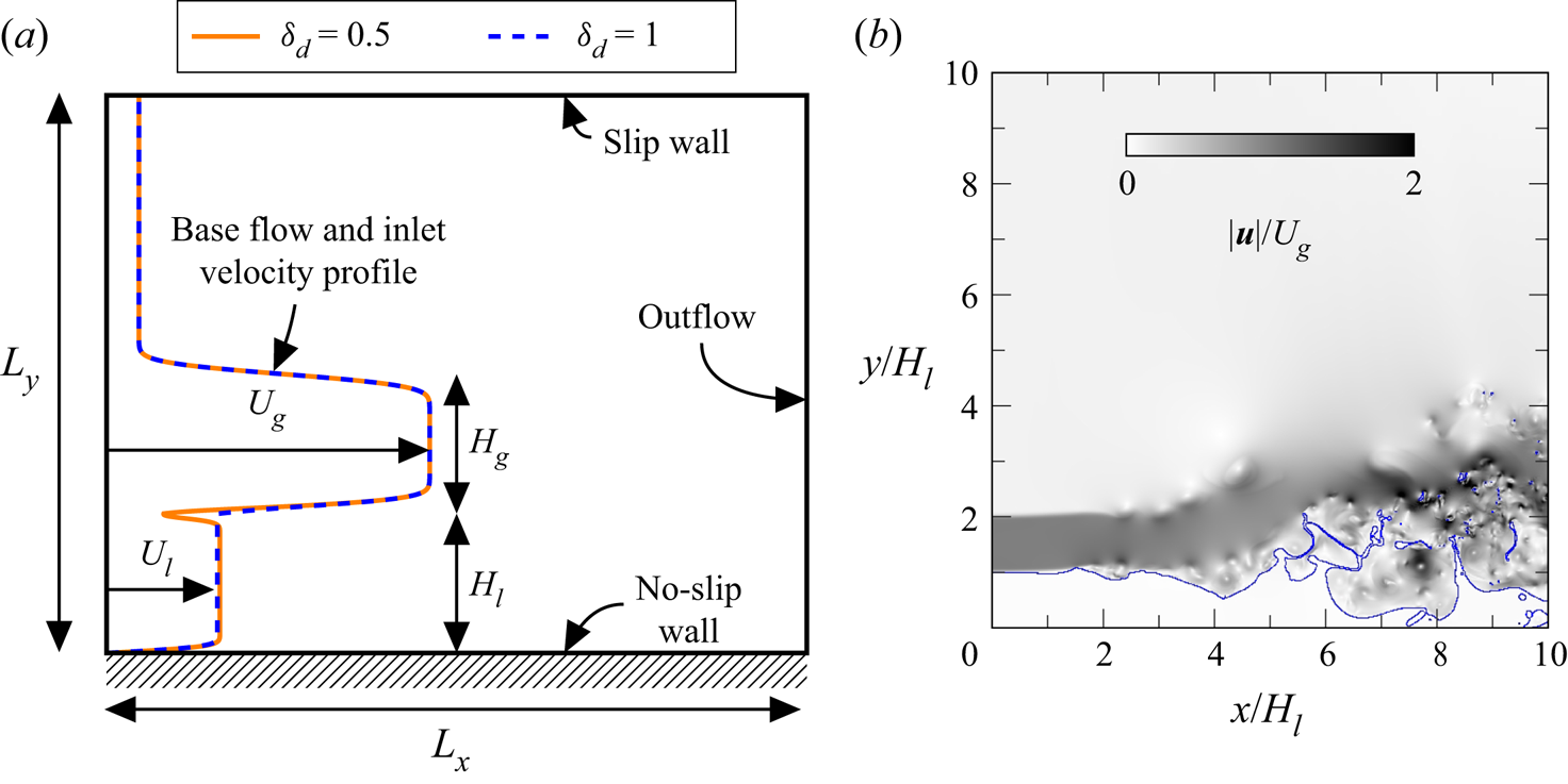
We study a wall-bounded air–water mixing layer corresponding to the configuration studied experimentally in Matas et al. (Reference Matas, Marty and Cartellier2011). The description of the numerical domain is presented in figure 1(a). A slow liquid stream with velocity  $U_l$, located above a wall, is placed below a fast gas stream with velocity
 $U_g$. Liquid and gas streams both have a finite thickness,
 $H_l$ and
 $H_g$, respectively. The domain is two-dimensional (2-D), with a velocity field defined as
 $\boldsymbol {u} = (u,v)$, where
 $u,v$ are the velocity components in the
 $x$ and
 $y$ directions, respectively, with
 $0 \leq x \leq L_x$ and
 $0 \leq y \leq L_y$.
(a) Sketch of the configuration. The deficit value  $\delta _d$ controls the initial shape of the velocity profile close to the interface. (b) Typical picture of the flow displaying the liquid–gas interface (blue line) and the velocity magnitude (greyscale).

The choice of a 2-D domain is motivated by the associated reduction of computational time and is justified at moderate gas velocity by the 2-D nature of the waves at their onset. Indeed, it can be seen in Ben Rayana, Cartellier & Hopfinger (Reference Ben Rayana, Cartellier and Hopfinger2006) (figure 3 of their paper), Fuster et al. (Reference Fuster, Matas, Marty, Popinet, Hoepffner, Cartellier and Zaleski2013) (figure 3 of their paper) and Matas et al. (Reference Matas, Marty, Dem and Cartellier2015) (figure 1 of their paper) that no significant transverse modulations of the waves can be seen at their onset. This, however, seems to be less the case at higher gas velocities, as seen in figure 7(a) of Matas et al. (Reference Matas, Marty, Dem and Cartellier2015). Note that purely spanwise modes are explored in Náraigh et al. (Reference Náraigh, Valluri, Scott, Bethune and Spelt2014) for density-matched periodic flows.
As suggested previously, we choose not to include the splitter plate separating the gas and liquid streams. This has two advantages: firstly, we avoid the simulation of the contact line dynamics on the splitter plate, which is expensive given the typical scales of the splitter plate; secondly we retain full control over the shape of the initial velocity profile. Linear stability (Otto et al. Reference Otto, Rossi and Boeck2013; Matas Reference Matas2015) has shown that the details of the velocity profile close to the interface and the finite thickness of the streams control the transition between convective and absolute regime, as well as the transition from confinement-induced to surface tension-induced absolute instability. In this study, we compare the results obtained using simulations, i.e. a fully nonlinear and global approach that allows for the development of the base flow, and linear stability analysis, i.e. a highly idealized approach that performs a local analysis of a parallel base flow subjected to infinitesimal perturbations. Both approaches are connected as the inlet velocity profile in simulations is also used as the base flow in the linear stability analysis.
The inlet velocity profiles are expressed as  $\boldsymbol {u}_{in} = \boldsymbol {u} (x=0,y) = (u(y),0)$. The expression for
 $u(y)$ depends on the vertical position. For
 $y \leq H_l$,
 \begin{equation} u(y) = \left\{ U_l \text{erf}\left(\frac{H_l-y}{\delta_l}\right) + U_i\left(1+\text{erf}\left (\frac{y-H_l}{\delta_d \delta_l}\right ) \right ) \right\} \times \text{erf}\left (\frac{y}{\delta_l}\right ) , \end{equation}
for  $H_l < y \leq H_g + H_l$,
 \begin{equation} u(y) = \left\{ \begin{aligned} & \left\{ U_g \text{erf}\left (\frac{y-H_l}{\delta_g}\right ) + U_i\left(1-\text{erf}\left (\frac{y-H_l}{\delta_d \delta_l}\right ) \right ) \right\}\\ & \quad \times \text{erf}\left (\frac{H_g+H_l - y}{\delta_g}\right ) + U_{sm}\left ( 1+ \text{erf}\left (\frac{y - (H_g+H_l)}{\delta_g}\right ) \right ) \end{aligned}\right. \end{equation}
and for  $y > H_g + H_l$,
 \begin{equation} u(y) = U_{sm}\left ( 1- \text{erf}\left (\frac{y - (H_g+H_l)}{\delta_g}\right ) \right ) + U_{cf}\text{erf}\left (\frac{y - (H_g+H_l)}{\delta_g}\right ). \end{equation}
In the previous expressions,  $\delta _g$ is the gas vorticity thickness,
 $\delta _l$ is the liquid vorticity thickness,
 $\delta _d$ is the dimensionless deficit parameter,
 $U_i$ is the interfacial velocity,
 $U_{cf}=0.1U_g$ is the coflow velocity and
 $U_{sm}=(U_{cf}+U_g)/2$ is the single-phase mixing layer velocity. The gas vorticity thickness is computed using the experimental correlation given in Matas et al. (Reference Matas, Marty and Cartellier2011):
 $\delta _g=6H_g/\sqrt {\rho _gU_gH_g/\mu _g}$. Note that, in the following, when
 $H_g$ is varied we do not vary
 $\delta _g$ but instead keep the value obtained using the previous relation for
 $H_g=1$ cm. The liquid vorticity thickness is constant and equal to
 $5\times 10^{-4}$ m. Following Otto et al. (Reference Otto, Rossi and Boeck2013), the interfacial velocity is defined based on tangential stresses continuity,
 $U_i = (U_g\mu _g/\delta _g + U_l\mu _l/\delta _l)/(\mu _l + \mu _g)\delta _d\delta _l$, with
 $\mu _l$ and
 $\mu _g$ the liquid and gas dynamic viscosities, respectively. The deficit parameter
 $\delta _d$ is used to control the magnitude of the interfacial velocity, therefore, the shape of the velocity profile around the liquid gas interface: if
 $\delta _d=1$, there is no velocity deficit, while a reduction of
 $\delta _d$ will induce a decrease of the interfacial velocity, as seen in figure 1(a). This velocity profile only differs from the one used for linear stability by the presence of a coflow used to provide the mass entrained by the high-speed gas (as in da Silva & Métais (Reference da Silva and Métais2002)). Note that one will exactly recover the velocity profiles used for linear stability analysis with
 $U_{cf}=0$.
The inlet velocity profile described by (2.1)–(2.3) is imposed at  $x=0$. Except stated otherwise, a uniformly random temporal perturbation of maximum amplitude
 $\alpha =10^{-5}\,\textrm {m}\,\textrm {s}^{-1}$ is introduced at
 $x=0$ on both components of the velocity in a band of width
 $\delta _g$ around the interface. A convective outlet boundary condition is imposed at
 $x=L_x$ (Orlanski Reference Orlanski1976). The convective velocity used in that condition is taken as the maximal speed in the vicinity of the outlet plane. The bottom boundary condition at
 $y=0$ is a no-slip wall, while the top boundary condition
 $y=L_y$ is a slip wall. The physical properties of air and water, as well as
 $\sigma$, the surface tension coefficient at an air–water interface, are taken as constant throughout this study and are presented in table 1. Gravity is taken into account, with
 $\boldsymbol {g} = (0, -9.81)\,\textrm {m}\,\textrm {s}^{-2}$ the gravity vector. The numerical domain is discretized with a uniform cell size,
 $\Delta x = \Delta y = \delta _g /n$, with
 $n$ to be specified later, for
 $y \leq 6H_l$. In the upper part of the domain, the mesh is progressively stretched in the vertical direction up to
 $y = L_y = 1.3L_x$ using a constant stretching ratio of
 $1.05$.
Physical properties of air and water.

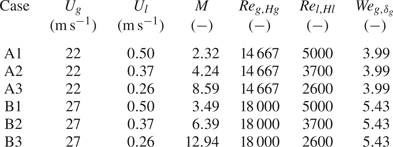
Finally, all the combinations of injection velocities used in this paper, as well as relevant non-dimensional parameters, are summarized in table 2 for the case where  $H_g=H_l=1$ cm. In all of § 4, we take
 $H_g=H_l=1$ cm. The additional non-dimensional parameters presented in table 2 are the gas stream Reynolds number,
 $Re_{g,Hg}=\rho _gU_gH_g/\mu _g$, the liquid stream Reynolds number,
 $Re_{l,Hl}=\rho _lU_lH_l/\mu _l$, and the gas stream Weber number,
 $We_{g,\delta _g}=\rho _gU_g^2\delta _g/\sigma$.
Summary of injection conditions and relevant non-dimensional parameters for  $H_g=H_l=1$ cm.

Note that, as there are several mechanisms behind the instability and several relevant velocity and spatial scales, wave frequency results are presented in a dimensional way in the rest of the paper.
3. Numerical methods
Fluid dynamics is governed by conservation laws. Assuming flow incompressibility ( $\boldsymbol {\nabla } \boldsymbol {\cdot } \boldsymbol {u} = 0$), conservation of mass gives
 \begin{equation} \frac{\partial \rho}{\partial t} + \boldsymbol{\nabla} \boldsymbol{\cdot} \left (\rho \boldsymbol{u} \right )= \frac{\partial \rho}{\partial t} + \boldsymbol{u} \boldsymbol{\cdot} \boldsymbol{\nabla} \rho = 0, \end{equation}
where  $\rho$ is the density field and
 $t$ is time. Multiphase momentum conservation is written in the framework of the one-fluid formulation: a single equation with space-varying material properties is used to describe the dynamics of both phases, e.g. see Tryggvason, Scardovelli & Zaleski (Reference Tryggvason, Scardovelli and Zaleski2011).
The effect of surface tension is added through a singular force,  $\boldsymbol {T}_{\sigma }$, acting at the interface. Momentum conservation thus gives
 \begin{equation} \frac{\partial \rho \boldsymbol{u}}{\partial t} + \boldsymbol{\nabla} \boldsymbol{\cdot} \left (\rho \boldsymbol{u} \otimes \boldsymbol{u} \right ) ={-} \boldsymbol{\nabla} p + \boldsymbol{\nabla} \boldsymbol{\cdot} \left ( \mu \left[ \boldsymbol{\nabla} \boldsymbol{u} + {\boldsymbol{\nabla} \boldsymbol{u}}^\textrm{T}\right ] \right) + \boldsymbol{T}_{\sigma} + \rho \boldsymbol{g}, \end{equation}
where  $p$ is the pressure and
 $\mu$ is the dynamic viscosity. In absence of phase change, the application of the momentum equation on the interface results in the classical jump condition for normal stress,
 \begin{equation} [p]_\varGamma = \sigma \kappa + 2[\mu ]_\varGamma \boldsymbol{n} ^\textrm{T}_{\varGamma} \boldsymbol{\cdot} \boldsymbol{\nabla} \boldsymbol{u} \boldsymbol{\cdot} \boldsymbol{n}_{\varGamma}, \end{equation}
where  $\kappa$ and
 $\boldsymbol {n}_{\varGamma }$ are the curvature and the normal vector to the interface
 $\varGamma$, respectively. The notation
 $[ \cdot ]_\varGamma$ represents the interfacial jump from liquid to gas. These equations are solved using NGA, a finite volume, staggered-grid flow solver (Desjardins et al. Reference Desjardins, Blanquart, Balarac and Pitsch2008).
Mass conservation, (3.1), is ensured through an unsplit semi-Lagrangian volume of fluid advection method (Owkes & Desjardins Reference Owkes and Desjardins2014) which allows us to obtain liquid volume fraction in each cell of the computational domain. Density and viscosity fields are computed from liquid volume fraction and the properties of each phase using arithmetic and harmonic averaging, respectively. The normal to the interface is computed using ELVIRA (Pilliod & Puckett Reference Pilliod and Puckett2004) and the interface is reconstructed using a piecewise linear interface calculation (Rider & Kothe Reference Rider and Kothe1998).
Momentum conservation, (3.2), is computed in a way consistent with mass transport and with the presence of interfacial discontinuities (Palmore & Desjardins Reference Palmore and Desjardins2019). Particularly, second-order centred schemes are used for spatial discretization for all terms but the convective term at the interface, where the consistent strategy is used (see Palmore & Desjardins (Reference Palmore and Desjardins2019) for more details). The coupling between velocity and pressure is enforced using an incremental pressure projection method (Goda Reference Goda1979) and time is advanced through an iterative Crank–Nicolson scheme (Teukolsky Reference Teukolsky2000).
Interface boundary conditions, (3.3), are included in the pressure through the use of a continuum-surface-force method (Francois et al. Reference Francois, Cummins, Dendy, Kothe, Sicilian and Williams2006). Interfacial curvature is computed using a combination of height function method (Popinet Reference Popinet2009) and least squares fit, in a way similar to Owkes et al. (Reference Owkes, Cauble, Senecal and Currie2018).
The present framework allows exact mass, momentum and kinetic energy conservation within each phase, while mitigating momentum and kinetic energy conservation errors at the interface even in the presence of high density or viscosity ratio, high shear or large exchange of kinetic energy.
Finally, the base flow for stability analysis is the inlet velocity profile, with  $U_{cf}=0$. The method used is the same as in Matas (Reference Matas2015). After superposition of a perturbation to the base flow and linearization, the perturbations are expanded into normal modes of the form
 $\boldsymbol {\tilde {u}}(k,y,\omega )\text {e}^{\text {i}(kx-\omega t)}$, with
 $k$ and
 $\omega$ the complex wavenumber and complex frequency, respectively. Gravity is taken into account. Integration of the resulting equations with a Runge–Kutta method is carried out from the solid wall in the liquid, and from a solid wall located at a distance
 $L_g$ in the gas phase, with
 $L_g$ much larger than the stream thicknesses, namely
 $L_g=30\max (H_g,H_l)$. The dispersion relation results from the connection of these integrated liquid–gas solutions at the interface via appropriate continuity of normal and tangential stresses.
The dispersion relation is solved for complex  $k$ using a shooting method, for fixed complex
 $\omega$. The absolute modes are then tracked using the Briggs criterion (Briggs Reference Briggs1964): we look for a pinching between branches (controlled by shear, confinement or surface tension) located in opposite sides of the
 $k$ half-plane at large
 $\omega _i$, with
 $\omega _i$ the imaginary part of the complex frequency. Particularly, this pinching must occur at positive
 $\omega _i$ for the instability to be considered as absolute, and
 $\partial \omega _r / \partial k_r$, the group velocity, is equal to zero at the pinching point, with
 $\omega _r$ and
 $k_r$ the real part of the complex frequency and wavenumber, respectively. The imaginary part of
 $k$,
 $k_i$, is the spatial growth rate.
4. Stability of an air–water mixing layer
4.1. General description
A typical flow picture displaying the liquid–gas interface and the velocity magnitude is presented in figure 1(b). Initially flat, the interface progressively deforms into a wavy shape. The liquid strongly interacts with the high-speed jet in the downstream part of the flow: the liquid jet gets thinner due to the transfer of momentum from gas to liquid and flow rate conservation, but one can also see large amplitude waves deviating the gas jet, as well as ligaments and liquid fragments pulled out by the jet. The gas–gas mixing layer shows the triggering of a Kelvin–Helmholtz instability. No recirculation is observed in the top part of the domain, showing that the coflow actually provides the mass entrained by the high-speed jet. The vertical position of the interface is sampled for all positions downstream of the inlet at a frequency of 10 000 Hz, allowing the study of the spatiotemporal development of the instability.
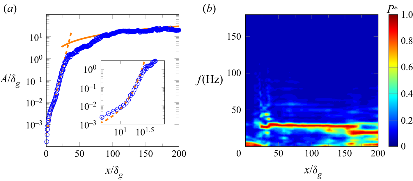
In figure 2(a), we show the spatial evolution of the wave amplitude, and in figure 2(b) the spectrogram of the interface height for case A2, with  $n=2$ and
 $\delta _d=1$. The wave amplitude is computed using the method presented in Matas et al. (Reference Matas, Marty and Cartellier2011): for a given downstream position, we construct a histogram of the interface positions over the sampling time and exclude the lowest and highest
 $0.5\,\%$. The remaining width of the histogram is taken as the amplitude
 $A$ of the waves. Several zones can be distinguished. Focusing on figure 2(a), one can see that for
 $20 \leq x/\delta _g \leq 50$, the computed amplitude (
 $\circ$, blue) seems to increase exponentially with downstream distance,
 \begin{equation} A= A_0 \textrm{e}^{k_i x}, \end{equation}
with, for figure 2(a),  $k_i=k_{i, exp}=323.2$ m
 $^{-1}$, where
 $k_{i, exp}$ is the value obtained experimentally (Matas et al. Reference Matas, Marty and Cartellier2011), as represented with a dashed line in figure 2(a).
Spatiotemporal development of the instability for the case A2 with  $n=2$,
 $\delta _d=1$. (a) Spatial evolution of the wave amplitude with: computed wave amplitude (
 $\circ$, blue); (4.1), with
 $A_0/\delta _g=3.8\times 10^{-4}$ and
 $k_i=k_{i,exp}=323.2$ m
 $^{-1}$ (orange dashed line); (4.2), with
 $C_0=0.21$ (orange solid line). The insert shows the same data in a log scale, with a close-up of the exponential growth region. (b) Spectrogram of the interface height.
 $P*$ is the normalized spectral power.

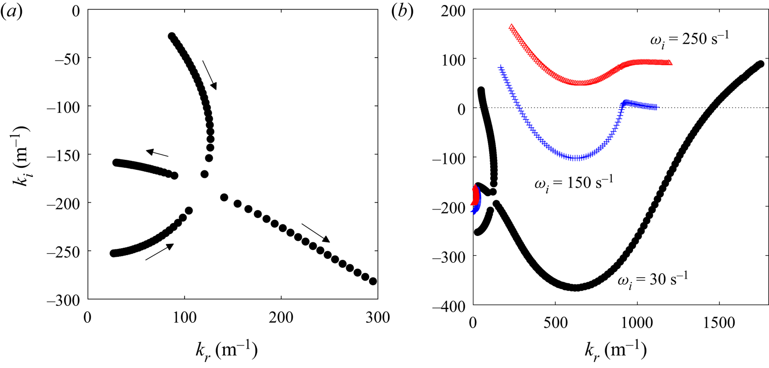
This observation has to be taken cautiously. The stability analysis predicts that the instability is absolute for these conditions, as seen on figure 3, where we see the pinching between the confinement branch, located close to the  $k_i$ axis, and the shear branch. Nonlinearity is therefore expected to quickly dominate, as the instability will grow exponentially in time and space. As the group velocity at the pinching point is zero, the predicted spatial growth rate has no clear meaning for the waves travelling downstream of the injector (Huerre & Monkewitz Reference Huerre and Monkewitz1990).
Spatial branches for case A2. (a) Pinching between confinement and shear branches, at  $\omega _i=30$ s
 $^{-1}$. The confinement branch is located close to the
 $k_i$ axis. The arrows indicate the direction in which
 $\omega _r$ increases. (b) Zoomed-out view of the pinch point showing the behaviour of the shear branch at low and large
 $k_r$ for
 $\omega _i=30$ s
 $^{-1}$, and for two additional values of
 $\omega _i$. At large
 $\omega _i$, the shear branch is located in the
 $k_i>0$ half-plane, while the confinement branch remains close to the imaginary axis in the
 $k_i<0$ half-plane: the two colliding branches therefore originate from opposite half-planes, in agreement with the Briggs criterion.

However, as said in the introduction, the predicted spatial growth rate controls the scale of oscillations in the cross-stream direction. The confinement branch is crossing the  $k_i$ axis around
 $-n{\rm \pi} /(2L)$, with
 $L$ the cross-stream characteristic length and
 $n=\{1,2,3,\ldots \}$. At the pinching point shown in figure 3,
 $k_{i,LSA} = - 180$ m
 $^{-1}$, which is close to
 $-{\rm \pi} /(2H_l)=-157$ m
 $^{-1}$, showing the matching between cross-stream perturbations and cross-stream confinement that leads to resonance, i.e. to absolute instability.
An exponential growth zone has been seen experimentally and numerically (Agbaglah et al. Reference Agbaglah, Chiodi and Desjardins2017; Ling et al. Reference Ling, Fuster, Tryggvason and Zaleski2019). Figure 2(a) shows that the wave growth obtained numerically is in agreement with the wave growth observed experimentally. The insert in figure 2(a) shows that the zone of exponential growth rate is extremely short, as seen in experiments.
The end of the previous zone occurs when the amplitude is of the order of the vorticity thickness, as observed in experiments. For  $x/\delta _g \geq 75$, the amplitude is growing linearly with downstream distance, following well the self-similar model of Hoepffner, Blumenthal & Zaleski (Reference Hoepffner, Blumenthal and Zaleski2011),
 \begin{equation} A = C_0\sqrt{\rho_g/\rho_l}U_g \tau, \end{equation}
with the characteristic time taken as  $\tau =x/U_D$, as in Marty (Reference Marty2015),
 $U_D$ is obtained using (1.2) and
 $C_0$ is a model constant to be specified. This model is represented by the continuous line in figure 2(a).
In figure 2(b), one can see the spatial evolution of the interface height spectra. For each location downstream of the inlet, we obtain the interface height spectrum and then normalize the spectral power by its local maximum. Note that we use the Welch method (Welch Reference Welch1967) to facilitate the extraction of the most amplified frequency, i.e. before taking its Fourier transform, we split the signal in 10 parts with a 60 % overlap between them, the resulting spectra are then averaged. A very clear frequency peak is observed and remains unchanged over a large extent of the domain, which may suggest the presence of a global mode of instability. Close to the outlet, lower frequency peaks are appearing.
In the next section, we detail the influence of the numerical parameters and the integration time on these results.
4.2. Assessment of the numerical methods
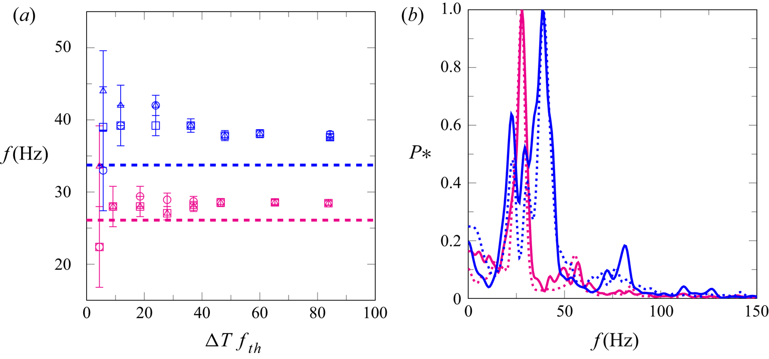
In figure 4(a), we show the influence of integration time on the most amplified frequency obtained at three downstream locations for two sets of injection conditions. The most amplified frequency is presented as a function of the normalized duration of the signal  $\Delta T f_{th}$, with
 $\Delta T$ the signal duration and
 $f_{th}$ the predicted wave frequency obtained by linear stability analysis. Note that the statistics are collected once the averaged height is stabilized over time. One can see that as soon as
 $\Delta T f_{th}$ is larger than
 $10$, i.e. approximately 10 waves have been generated, the variations of the most amplified frequency in time and space are of the order of the spectral resolution. This is in agreement with the results of Agbaglah et al. (Reference Agbaglah, Chiodi and Desjardins2017). For both cases, the most amplified frequency is stable in time, and with the increase of spectral resolution all measured frequencies become perfectly independent of the position, providing that the latter is in the interval
 $25 \leq x/\delta _g \leq 150$. In order to reduce the uncertainty on the frequency value an integration time of
 $\Delta T f_{th}\geq 40$ would be ideal, but this choice will be more difficult to achieve for 3-D simulations, or even very resolved 2-D simulations. The present analysis shows that even an integration time of
 $\Delta T f_{th}\sim 10$ is sufficient to obtain a good estimate of the frequency.
Dependence of frequency measurements on integration time and domain length for  $n=2$,
 $\delta _d=1$. (a) Spatiotemporal convergence of the most amplified frequency with: Blue, case B1; magenta, case A2;
 $x/\delta _g=44$ (
 $\circ$);
 $x/\delta _g=67$ (
 $\triangle$);
 $x/\delta _g=89$ (
 $\square$). The error bars represent the spectral resolution. Horizontal dashed lines are the theoretical frequency for each case. (b) Dependence of frequency spectra on domain length for
 $\Delta Tf_{th}=40$,
 $x/\delta _g=89$ with: case B1 (Blue); case A2 (magenta); continuous line,
 $L_x/\delta _g=240$; dotted line,
 $L_x/\delta _g=320$.

In figure 4(b), we show the impact of domain length on the frequency spectra for two sets of injection conditions. Our tests show that, for the cases of figure 4(b), the most amplified frequency is not affected by the position of the outlet boundary condition once  $L_x/\delta _g$ is larger than
 $240$, which has been confirmed for other cases (results not shown). We will therefore ensure that this condition is met for all cases.
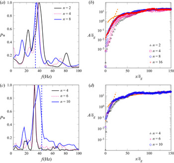
In figure 5, we show the effect of resolution on the spatiotemporal development of the instability for case  $B1$ and two values of the deficit parameter. In figure 5(a) is presented the evolution of the frequency spectra with
 $n$ (
 $=\Delta x/\delta _g=\Delta y/\delta _g$), the resolution, for
 $\delta _d=1$. We see that, as the mesh is refined, the most amplified frequency approaches the theoretical value. The error on the finest mesh, here
 $n=8$, is only
 $4.6\,\%$, while the error for the coarsest resolution,
 $n=2$, is
 $12\,\%$. In figure 5(b), the convergence of the amplitude with mesh resolution for
 $\delta _d=1$ is shown. From
 $n=2$ (
 $\triangle$, black) to
 $n=16$ (
 $+$, red) the amplitude is mostly affected by the resolution in the area close to the injector, where the amplitude is small. Far from the inlet, i.e.
 $x/\delta _g \geq 75$, the amplitude is essentially not affected by resolution and closely follows the self-similar model. Mesh resolution mostly affects the location at which the amplitude reaches this self-similar region. This location is shifted closer to the injector as the mesh is refined. Note that the amplitude is essentially not modified between
 $n=8$ and
 $n=16$, meaning that we reach independence from mesh resolution. Note also that, close to the injector, we do again see a zone of exponential growth, with a slope equal to the one observed experimentally for these injection conditions. As the mesh is refined, the transition between the inlet of the domain and the zone of exponential growth progressively disappears, which is not the case in experiments (Matas et al. Reference Matas, Marty and Cartellier2011) or simulations including a splitter plate (Agbaglah et al. Reference Agbaglah, Chiodi and Desjardins2017; Ling et al. Reference Ling, Fuster, Tryggvason and Zaleski2019).
Effect of mesh resolution on the instability characteristics for case B1 and two values of the deficit parameter. In the zone of interest,  $\Delta x = \Delta y = \delta _g /n$. All spectra are taken at
 $x/\delta _g= 67$, with
 $\Delta T f_{th} \geq 20$. (a) Convergence of frequency with mesh resolution for
 $\delta _d=1$. The vertical dashed line represents the corresponding theoretical frequency. (b) Convergence of wave amplitude with mesh resolution for
 $\delta _d=1$ with: (range dashed line), (4.1), with
 $A_0/\delta _g=0.016$ and
 $k_i=k_{i,exp}=569.9$ m
 $^{-1}$; (orange solid line) (4.2), with
 $C_0=0.21$. (c) Similar to (a), with
 $\delta _d=0.5$. (d) Similar to (b), with
 $\delta _d=0.5$,
 $A_0/\delta _g=0.046$ and
 $C_0=0.27$. Note that in (b,d), only one data point every six is shown to enhance readability.

In figure 5(c), we present the evolution of the frequency spectra with mesh resolution for  $\delta _d=0.5$ and the same B1 case. Again, one can see that, as the mesh is refined, the most amplified frequency converges towards the predicted value, but the error on the finest resolution,
 $n=10$, is still
 $12\,\%$. The evolution of amplitude with resolution for
 $\delta _d=0.5$ is shown in figure 5(d). Similarly to the case without velocity deficit, we can see that as the mesh is refined, the position at which the amplitude enters the self-similar region is shifted towards the inlet. In the exponential growth region, we are again in very good agreement with the slope measured experimentally by Matas et al. (Reference Matas, Marty and Cartellier2011). Note that we do observe that the self-similar growth region is affected by the reduction of
 $\delta _d$ as we had to increase
 $C_0$ from
 $0.21$ to
 $0.27$ in order to obtain a good agreement between the computed amplitude and (4.2) in the downstream area. This is consistent with our observation of a decrease in the wave speed with the decrease of
 $\delta _d$ (results not shown). This suggests, as already pointed out by Marty (Reference Marty2015), that one needs to adjust the velocity scale used in (4.2) to the variations of the interfacial wave speed, therefore, to the details of the velocity profile, in order to obtain a good self-similarity of the wave amplitude.
Overall, we find that the influence of the velocity deficit  $\delta _d$ is expensive to capture and the systematic study of its influence on the simulation results is left for future work. For the rest of this work, we will only consider the
 $\delta _d=1$ case in simulations. Nonetheless, we wish to comment on the reason for this difficulty. As pointed out by Otto et al. (Reference Otto, Rossi and Boeck2013), and seen in figure 1(a), the presence of an interfacial velocity deficit induces the presence of a minimum in the velocity profile, in our case on the liquid side, around which the shear changes sign. Depending on the value of
 $\delta _d$ and other injection parameters, this minimum can move very close to the interface. In our case this minimum is located at a distance of
 $238\,\mathrm {\mu }$m from the interface, hence a distance two times smaller than the vorticity thickness. Reducing
 $\delta _d$ or
 $M$ can make this minimum move even closer to the interface (Otto et al. Reference Otto, Rossi and Boeck2013). The position of this minimum and the associated shear are very expensive to capture in simulations, hence the difficulty to capture the effect of
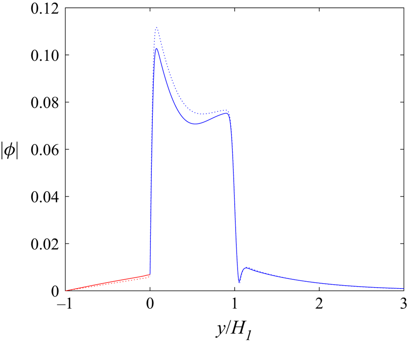
 $\delta _d$. Unlike the case of convective modes presented in Bagué et al. (Reference Bagué, Fuster, Popinet, Scardovelli and Zaleski2010), we do not observe the presence of extremely sharp variations of the eigenfunctions associated with the mode of instability, as can be seen on figure 6, where we show
 $|\varPhi |$, the norm of the stream function computed by the stability analysis for case
 $B1$ and for two values of
 $\delta _d$:
 $\delta _d=1$ (dashed line) and
 $\delta _d=0.5$ (continuous line), as a function of the vertical coordinate. The stream function is related to the vertical velocity perturbation:
 $\partial \varPhi /\partial x= \tilde {v}(k,\omega,y)\text {e}^{\text {i}(kx-\omega t)}$. No significant difference is observed between both cases, except a slightly higher value of
 $|\varPhi |$ in the gas stream for
 $\delta _d=1$. Thus, we think that the difficulty associated with the resolution of the velocity deficit is solely due to the difficulty of resolving the velocity minimum position and the associated shear, rather than to an increase in the eigenfunctions sharpness. Note that this comment only applies to confinement-induced absolute modes which occur at low wavenumbers (Matas Reference Matas2015).
Absolute value of the stream function eigenfunction for case B1 with  $H_g=H_l=1$ cm: Dotted line,
 $\delta _d=1$ (
 $k=140+170i$ m
 $^{-1}$,
 $\omega =209+30i$ s
 $^{-1}$); continuous line,
 $\delta _d=0.5$ (
 $k=135+195i$ m
 $^{-1}$,
 $\omega =272 +35i$ s
 $^{-1}$); red, liquid side; blue, gas side. The horizontal axis is shifted so that the
 $y=0$ location corresponds to the interface location.

This mesh convergence study shows that, focusing on the case where no interfacial velocity deficit is introduced, a resolution  $n=8$ allows a converged amplitude and a very low error on the frequency value. We will therefore choose this resolution in § 4.3 where we will compare simulation results obtained for all cases presented in table 2. However, the previous mesh convergence study also shows that a resolution
 $n=2$ leads to an acceptable error on the frequency, as well as an amplitude that follows the self-similar growth model. We will therefore choose
 $n=2$ in § 5, devoted to the analysis of the effect of confinement on the stability of the flow.
We have thus established the performance and the limits of our numerical methods, which could be useful for the development and validation of future methods. We now switch to the use of the solver to demonstrate convergence between simulations, linear theory and experiments on confinement-induced absolute modes.
4.3. Convergence between simulation, linear theory and experiments
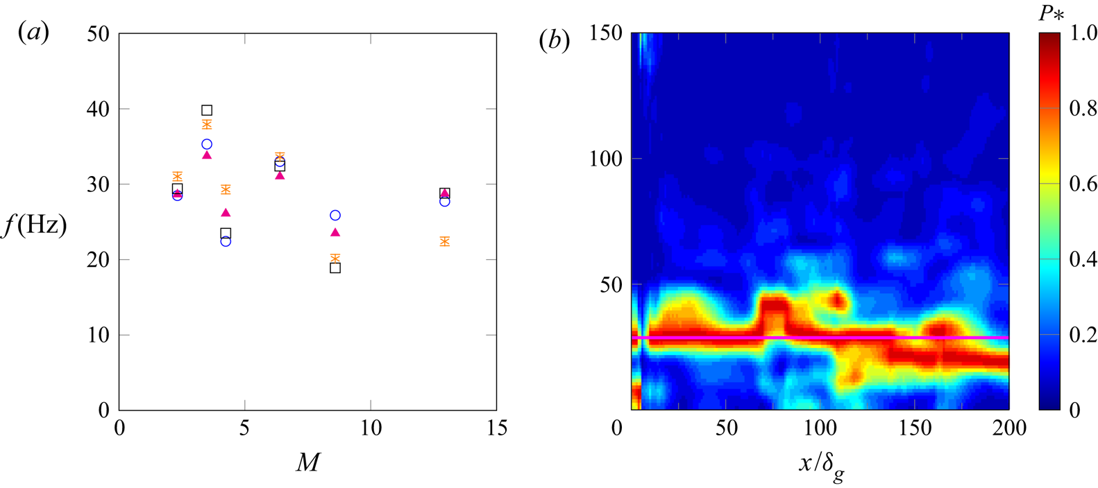
In figure 7(a), we show the evolution of the most amplified frequency obtained numerically, for  $n=8$ (
 $\circ$, blue) and
 $n=2$ (
 $\ast$, orange), as a function of the dynamic pressure ratio and for all cases of table 2. We plot the numerical results along with the most amplified frequency obtained with linear stability analysis (
 $\triangle$, magenta). For all cases of table 2, the stability analysis predicts that the instability is absolute, driven by a resonance of the shear instability within the confined streams (confinement mechanism). We also add for reference the experimental results of Matas et al. (Reference Matas, Marty and Cartellier2011) (
 $\square$, black).
(a) Most amplified frequency of the interface height signal as a function of the dynamic pressure ratio for all cases of table 2 with: experimental results (Matas et al. Reference Matas, Marty and Cartellier2011) ( $\square$, black); linear stability analysis results (
 $\triangle$, magenta); simulation results with
 $n=2$ (
 $\ast$, orange); simulation results with
 $n=8$ (
 $\circ$, blue). (b) Spectrogram of the interface height signal for case
 $A1$, with
 $n=8$. The horizontal magenta line represents the predicted wave frequency.

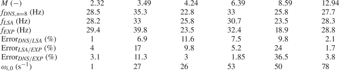
The frequency values obtained by simulations ( $n=8$), stability analysis and experiments are summarized in table 3, along with the error level between the different approaches and the values for each case of the temporal growth rate at the pinching point,
 $\omega _{i,0}$, also called the absolute growth rate.
Comparison between wave frequency values obtained using simulations, stability analysis and experiments, error between the three approaches, and absolute growth rates for each case.

The comparison between stability analysis, simulations and experiments has to be split in two parts. First, the comparison between stability analysis and simulations, which are directly connected as the inlet velocity profile in simulations is the base flow used in stability analysis, presents a maximal level of error of 11.6 %. This is very satisfactory. The remaining difference might be explained by nonlinearities, spatial variations of the velocity profile or by subtle numerical errors.
Secondly, the comparison of the two previous approaches (simulations and stability analysis) with experiments presents a maximum error of 36.5 % on wave frequency value. Many choices in the modelling can explain such discrepancies, e.g. shape of the velocity profile (which includes velocity deficit value, vorticity thicknesses values, use of  ${\rm erf}$ functions), turbulence intensity, nonlinearities, 3-D effects, as well as measurements errors. Given the complexity of the phenomenon, we consider that an average error level of 10 % and a maximum error level of less than 40 % between simulations/stability analysis and experiments is satisfactory.
As shown in table 3, we note that the case with the lowest absolute growth rate corresponds to a case where the agreement between the three approaches is extremely satisfactory. An absolute instability growing exponentially in space and time, the previous observation is not surprising as the case with the lowest absolute growth rate may correspond to the case where nonlinear effects will take the longest before they dominate (as will also be seen in the study of wave amplitude). For the other cases, no correlation seems to emerge between  $\omega _{i,0}$ and the error between the three approaches, but we note that these five cases are farther from the neutral boundary curve (
 $\omega _{i,0}=0$ s
 $^{-1}$).
To go further in the comparison, one could attempt a global stability study, or several local stability analyses, by taking into account the spatial variations of the base flow, as done for example in Juniper et al. (Reference Juniper, Tammisola and Lundell2011) and Biancofiore et al. (Reference Biancofiore, Gallaire and Pasquetti2011), or directly using nonlinear mean flows, as done for example in Oberleithner, Rukes & Soria (Reference Oberleithner, Rukes and Soria2014). This is something that we have attempted, but we faced difficulties in fitting velocity profiles obtained from simulations by velocity profiles that would still be in the family of velocity profiles described by (2.1)–(2.3). We therefore leave this approach for future work.
This favourable comparison between all approaches is a significant result because it shows that, while the level of error may vary between cases, we do observe convergence between simulation, linear stability analysis and experiment on cases where the instability is triggered by confinement.
The inclusion of the finite thickness of liquid and gas streams in the stability analysis has been shown to allow the convergence between experiments and linear stability analysis (Matas Reference Matas2015; Matas et al. Reference Matas, Delon and Cartellier2018); here we confirm for the first time its impact through simulations. Our work is, therefore, highly complementary to the one presented in Fuster et al. (Reference Fuster, Matas, Marty, Popinet, Hoepffner, Cartellier and Zaleski2013), which showed convergence between simulation, linear stability analysis and experiments on surface tension-induced absolute instabilities. In § 5, we will give further evidence of the destabilizing influence of confinement.
In figure 7(b), we show a spectrogram of the interface height signal for case A1 with  $n=8$. One can see that the most amplified frequency is not perfectly constant with downstream distance, but that it matches the theoretical value for more than half of the spatial locations. We can thus question the appearance of such small spatial variations of the most amplified frequency. A possibility would be to question the local or global nature of the mode of instability (Huerre & Monkewitz Reference Huerre and Monkewitz1990). The frequencies predicted by linear stability analysis correspond to the stability property of the inlet velocity profile, but do not give information of whether the predicted absolute mode is local or global. However, it is observed experimentally that the most amplified frequency does not vary with downstream distance (Matas et al. Reference Matas, Marty and Cartellier2011), i.e. that the absolute mode is global. We observed in our simulations that those spatial frequency variations are increasing with resolution. Therefore, we postulate instead that this is an effect of the 2-D nature of the simulation, and particularly of the 2-D nature of the turbulence. Note that a decrease of frequency with downstream distance has already been observed for similar 2-D configurations with moderate density ratios, and was attributed to vortex pairing (Fuster et al. Reference Fuster, Bagué, Boeck, Le Moyne, Leboissetier, Popinet, Ray, Scardovelli and Zaleski2009) or wave merging (Valluri et al. Reference Valluri, Naraigh, Ding and Spelt2010). A way to improve the understanding of spatial frequency variations would be to perform a mesh convergence in three dimensions under experimental conditions, but this task is made difficult by its very high computational cost.
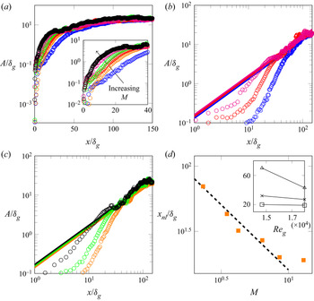
In figure 8, we present a comparison of the wave amplitude evolution for the cases of table 2. In figure 8(a), one can see that for all cases studied, the amplitude follows a similar evolution as the one described in § 4.1. The main differences in terms of amplitude are found for  $x/\delta _g \leq 50$, where we see that, for the range of injection conditions under study, the amplitudes are sorted with the dynamic pressure ratio, as detailed by the insert in figure 8(a). Interestingly, one can also note that the absolute growth rate is also increasing with
 $M$, see table 3. This relation between downstream wave amplitude evolution and absolute growth rate is not surprising as an absolute instability is growing exponentially in space and time. This effect of the dynamic pressure ratio on the near injector amplitude is coherent with the creation of a potential liquid cone that shortens with
 $M$ (Raynal Reference Raynal1997). Downstream of this zone, the amplitudes are closer to each other, but clearly follow a linear growth with downstream distance, as predicted by (4.2). To further examine this zone of linear growth, we present in figures 8(b) and 8(c) the evolution of the amplitude at fixed gas Reynolds number,
 $Re_g=14\,667$ and
 $Re_g=18\,000$, respectively, and for the three values of the liquid Reynolds number used in this study. In both of those figures, we add the self-similar growth model, (4.2), for comparison. The agreement with simulation results is very good. Remarkably,
 $C_0$ is constant for all plots, and the differences in the slopes are only due to the change in injection conditions, showing a clear self-similarity of the wave amplitude. This was not the case in the experiments of Marty (Reference Marty2015), where
 $C_0$ had to be adjusted to fit the experimental results. This is consistent with our observation of § 4.2: when the wave speed changes, some corrections have to be applied to the velocity scale used in (4.2). Since all the cases simulated in this section correspond to confinement-induced absolute modes, the wave velocity is close to
 $U_D$, which is in agreement with the inviscid mechanism driving the instability (Matas Reference Matas2015), therefore, no correction is needed in the self-similar growth model.
Comparison of wave amplitude for all cases of table 2, for  $n=8$ with A1 (
 $\circ$, blue); A2 (
 $\circ$, red); A3 (
 $\circ$, magenta); B1 (
 $\circ$, orange); B2 (
 $\circ$, green), B3 (
 $\circ$, black). (a) evolution of the amplitude for all 6 cases. The insert shows the same data with a zoom in on the inlet area. (b) Evolution of the amplitude for
 $Re_g=14\,667$. (c) Evolution of the amplitude for
 $Re_g=18\,000$. In (b,c), the solid lines correspond to the self-similar growth model, (4.2), with the same colour code as the symbols and
 $C_0=0.21$. (d) Evolution of the position of entry in the nonlinear regime as a function of the dynamic pressure ratio for all cases of table 2 (
 $\square$, orange). The dashed black line corresponds to a
 $1/M$ scaling. The insert shows the same data plotted as a function of the gas Reynolds number with:
 $Re_l=2600$ (
 $\square$);
 $Re_l=3700$ (
 $\times$);
 $Re_l=5000$ (
 $\triangle$). Note that in (a–c), only one data point in every six is shown to enhance readability.

In figure 8(d) we present the position of entry in the self-similar region as a function of the dynamic pressure ratio. For the range of injection conditions studied here, one can see that the position of entry in the self-similar zone appears to scale as  $1/M$. We also plot this position as a function of the gas Reynolds number, which shows that the impact of the liquid Reynolds number increases when the gas Reynolds number is reduced. Note that, in figure 5(d), one can observe that the decrease of
 $\delta _d$ seems to induce an earlier entry in the nonlinear growth region.
In summary, we have demonstrated the agreement between linear theory, simulations and experiments on wave frequency value in case of confinement modes, which validates the role of confinement in the stability of an air–water mixing layer. We have also shown the consistency between simulations and experiments on wave growth, as well as a verification of the self-similar model for nonlinear wave growth of Hoepffner et al. (Reference Hoepffner, Blumenthal and Zaleski2011).
5. Exploring the effect of confinement
In this section we explore in greater detail the effect of gas and liquid stream confinement on the stability of the flow. We first prove that confinement is indeed one of the mechanisms driving the transition between convective and absolute instabilities (along with the interfacial velocity value). We then discuss the effects of confinement, symmetric or non-symmetric, on the characteristics of the instability. For this part, we exclusively study cases A1 and B2. All parameters but  $H_g$ and
 $H_l$ are kept constant and equal to the values used in the previous section. In particular, note that the gas vorticity thickness
 $\delta _g$ is kept constant equal to its value obtained for
 $H_g=1$ cm.
5.1. Convective/absolute transition
As already said in the introduction, convectively unstable flows behave as noise amplifiers, i.e. the response of the system depends on the injected perturbations, whereas absolutely unstable flows behave as oscillators, i.e. the response of the system does not depend on the injected perturbations (Huerre & Monkewitz Reference Huerre and Monkewitz1990).
In order to apply those notions to our study, we first focus on case B2, with  $H_g=H_l=H$, i.e. a symmetric confinement. We study two values of
 $H$, namely
 $H=1$ cm and
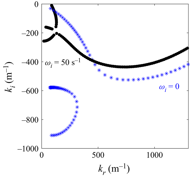
 $H=0.25$ cm. We show in figure 9 that the flow is predicted by linear stability analysis to be absolutely unstable for
 $H=1$ cm (
 $\bullet$) and convectively unstable for
 $H=0.25$ cm (
 $*$, blue). In the case of the absolute mode, a pinching occurs at low wavenumber (and positive
 $\omega _i$) between confinement and shear branches. For the convective mode, the most unstable mode of the shear branch, corresponding to the largest
 $|k_i|$, is located at a higher wavenumber. For
 $H=0.25$ cm (
 $*$, blue), the confinement branch can be seen close to the imaginary axis but no pinching occurs with the shear branch.
Spatial branches for case B2 with:  $H=1$ cm (
 $\bullet$) and
 $H=0.25$ cm (
 $*$, blue).

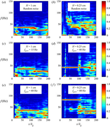
In figure 10, we examine the spectrograms of the instability for these two values of  $H$ and different injected perturbations. We choose a uniformly random, low-amplitude perturbation (figure 10a,b), as in the previous section, and a deterministic perturbation
 $f'=10^{-3} \sin (2{\rm \pi} f_{pert} t)$ (figure 10c–f), with
 $f_{pert}$, the perturbation frequency to be specified later.
Noise amplifier versus oscillator behaviour; case B2,  $n=2$. Spectral resolution is
 $0.56$ Hz for all spectrograms. Here (a,c,e)
 $H=H_g=H_l=1$ cm and (b,d, f)
 $H=H_g=H_l=0.25$ cm. (a,b) Random noise of amplitude
 $10^{-5}$. (c–f) Deterministic noise of amplitude
 $10^{-3}$ and
 $f_{pert}={15;40;60;80}$ Hz for the cases (c–f), respectively. The colour scale corresponds to the normalized spectral power.

One can see that when the mode is predicted to be absolute ( $H=1$ cm, figure 10a,c,e), the spectrograms are barely modified by the injected perturbations. The injected deterministic perturbation can be seen in figures 10(c) and 10(e), only very close to the inlet (
 $x/\delta _g \leq 5$). Farther downstream, the flow has its own dynamics, and the most amplified frequency and its variations are not affected by the injected perturbation.
On the other hand, when the mode is predicted to be convective ( $H=0.25$ cm, figure 10b,d, f), the spectrograms look very different depending on the injected noise. In the case of a random, low-amplitude perturbation, shown in figure 10(b), the most amplified frequency is more difficult to extract as it varies spatially. This behaviour had already been seen in Fuster et al. (Reference Fuster, Bagué, Boeck, Le Moyne, Leboissetier, Popinet, Ray, Scardovelli and Zaleski2009), where it is also said that for the case of convectively unstable flows, the comparison between local linear stability analysis and simulations has to be restricted to the linear growth region, i.e. where the linear stability analysis makes sense. In this area, around
 $x/\delta _g = 25$, the most amplified frequency is of
 $73$ Hz. Farther downstream, the most amplified frequency is progressively decreasing. For the cases with a deterministic perturbation injection, shown in figures 10(d) and 10( f), one can see that the forcing frequency is the most amplified in more than half of the domain, showing that the stability of the flow does actually depend on the injected perturbation.
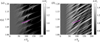
Another way to illustrate that we capture a convective/absolute transition driven by confinement is by constructing a spatiotemporal diagram of the interface height, also called a Hovmöller diagram, as used in Odier et al. (Reference Odier, Balarac, Corre and Moureau2015) and Odier, Balarac & Corre (Reference Odier, Balarac and Corre2018). As shown in figure 9, in the confinement-induced absolute mode, the pinching point occurs at a low wavenumber, whereas in the case of convective mode, the most amplified wavenumber is much higher. This difference can also be seen through the Hovmöller diagram of the instability. In figure 11, we show, for case B2 and a random inlet forcing, two spatiotemporal diagrams of the interface height for the same time window and two values of  $H$:
 $H=1$ cm (figure 11a) and
 $H=0.25$ cm (figure 11b). One can see that the main difference between both plots is in the wavelength. The waves are much shorter for
 $H=0.25$ cm than for
 $H=1$ cm which is consistent with the much larger predicted wavenumber for these conditions. For
 $H=1$ cm we have
 $\lambda \approx 4H$, whereas for
 $H=0.25$ cm we have
 $\lambda \approx 0.25H$.
Spatiotemporal diagrams of the interface height. Case B2,  $n=2$ with a low amplitude random forcing at the inlet. Here (a)
 $H=H_g=H_l=1$ cm; (b)
 $H=H_g=H_l=0.25$ cm. The magenta line corresponds to a wave speed equal to
 $U_D$, i.e.
 $U_{\phi }=U_D=1.30\,\textrm {m}\,\textrm {s}^{-1}$.

According to the energy budget presented in Matas (Reference Matas2015), the absolute mode induced by confinement is driven by inviscid stresses, whereas the convective mode is fed by the work of tangential viscous stresses on the interface. This difference can also be seen by examining the effect of  $H$ on the wave speed. In figure 11, we add on both plots a magenta line corresponding to a wave speed equal to
 $U_D$. For
 $H=1$ cm (figure 11a), this value is in agreement with the numerical result, which may be interpreted as an argument in favour of an inviscid mechanism, as suggested by Matas (Reference Matas2015). On the other hand, for
 $H=0.25$ cm (figure 11b), the agreement between the numerical results and
 $U_D$ is less favourable.
These three previous arguments (noise amplifier versus oscillator behaviour; wavenumber value; wave speed) demonstrate that the transition from the convective to the absolute mode is indeed induced by confinement, as predicted by linear stability analysis, and is fully captured numerically. A large wavelength of the order of the injector size and a wave speed close to Dimotakis’ may be good indicators of the presence of confinement modes.
5.2. Effect of confinement on the stability of the flow
In the previous section we confirmed the transition between convective and absolute modes due to flow confinement. We now study the impact of confinement, symmetric or not, on the characteristics of the instability, i.e. frequency and amplitude. We remind the reader that we focus on cases A1 and B2, where we only vary the thicknesses of the gas and liquid streams,  $H_g$ and
 $H_l$, respectively, while keeping all other parameters constant. We first start by considering the effect of
 $H$ for a symmetric confinement,
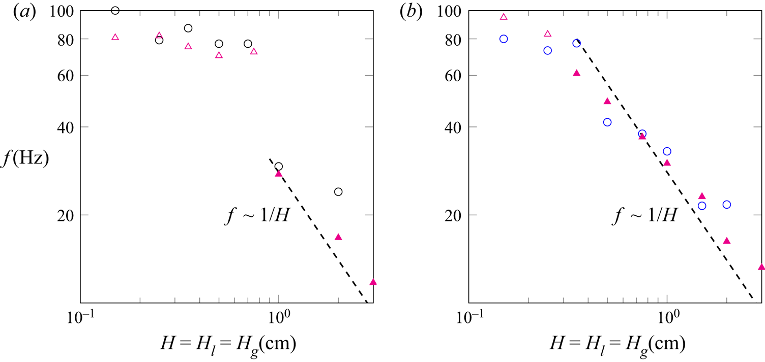
 $H_g=H_l=H$, on the most amplified frequency, shown in figure 12.
Case of a symmetric confinement: effect of  $H$ on the most amplified frequency (
 $n=2$). (a) Simulation results for case A1 (
 $\circ$, black), (b) simulation results for case B2 (
 $\circ$, blue). In both plots the triangles correspond to the frequency predicted by linear stability, with an open symbol for a convective mode and a filled symbol for an absolute mode due to confinement. Spectral resolution is of 0.56 Hz for all simulation results. Dashed lines correspond to a
 $1/H$ scaling.

First, one can observe that the overall agreement between linear stability analysis and simulations is very satisfactory, in convective as well as in absolute regimes.
One can observe that, when reducing  $H$, case A1 (
 $M=2.32$) presents a transition from absolute to convective regimes for
 $H$ between
 $0.75$ cm and
 $1$ cm. On the other hand, case B2 (
 $M=6.39$) presents the same behaviour for
 $H$ between
 $0.25$ cm and
 $0.35$ cm. These results suggest that the transition from convective to confinement-induced absolute instabilities does depend on the injection condition, i.e. the value of
 $M$, as well as on the confining geometry. In other words, when increasing
 $M$, the flow may be absolutely unstable for a larger range of stream thicknesses.
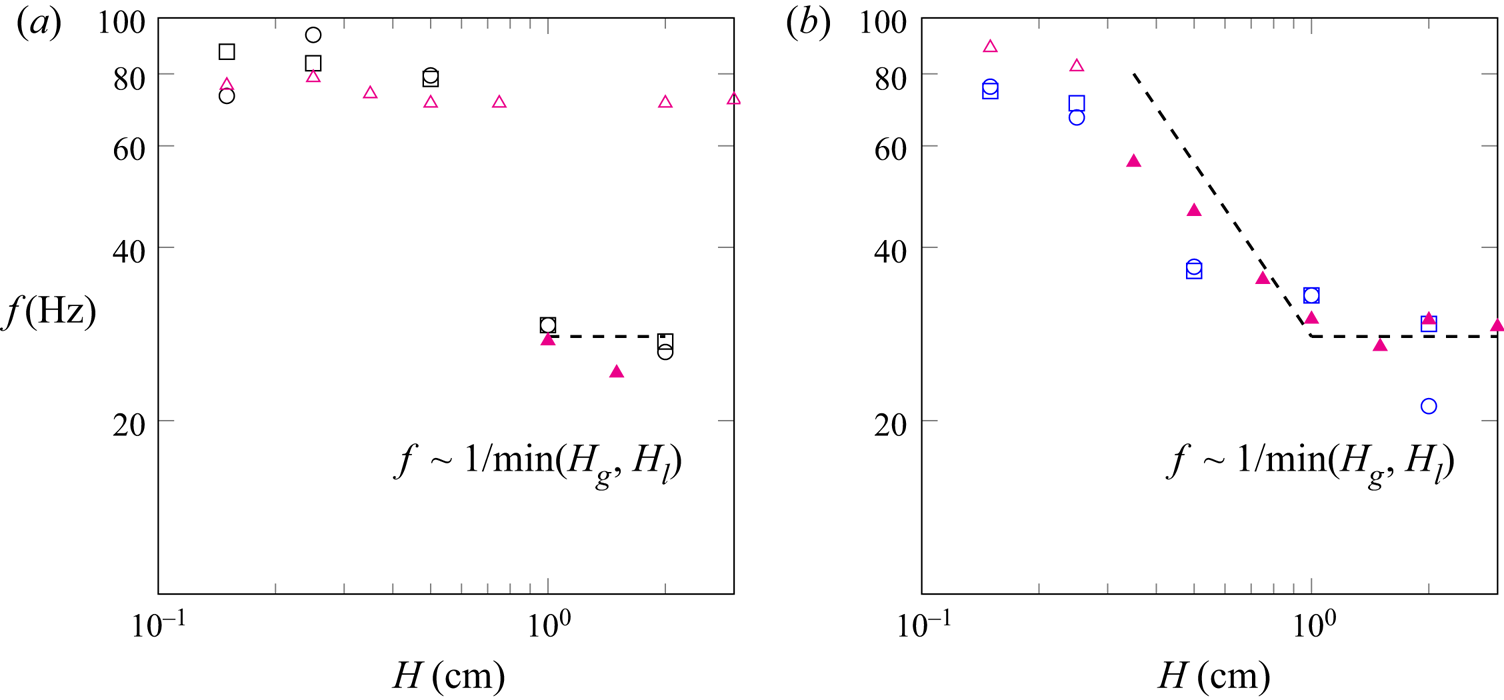
In figure 13, we show the evolution of the most amplified frequency in the case of non-symmetric streams, i.e. we keep one stream thickness constant while varying the other one. In figure 8 of Matas (Reference Matas2015), it is shown through stability analysis that both thicknesses have symmetric effects on the location of the pinching point, which may be surprising as a flow with a thin gas stream and a large liquid stream could seem very different from a flow with a thick gas stream and a thin liquid stream. This can be related to the symmetry found in the dispersion relation for the sinuous mode of a double shear layer in Juniper (Reference Juniper2006). Here we do confirm this symmetric behaviour through simulations: one can see in figure 13 that in most cases, the results for  $H_g=1$ cm,
 $H_l=H$ (symbols
 $\circ$ and
 $\circ$, blue) and
 $H_g=H$,
 $H_l=1$ cm (symbols
 $\square$ and
 $\square$, blue) are in agreement. For
 $H \leq 1$ cm, the most amplified frequencies are very similar to the ones presented in figure 12 for the case of symmetric streams, i.e.
 $H_g=H_l$. Above
 $H=1$ cm, and in case of absolute mode, the most amplified frequency appears to be constant with
 $H$, which is not the case for a symmetric confinement (see figure 12).
Case of a non-symmetric confinement: effect of  $H$ on the most amplified frequency (
 $n=2$). (a) Case A1, simulation results with
 $H_g=1$ cm and
 $H_l=H$ (
 $\circ$, black); simulation results with
 $H_g=H$ and
 $H_l=1$ cm (
 $\square$, black). (b) Case B2, simulation results with
 $H_g=1$ cm and
 $H_l=H$ (
 $\circ$, blue), simulation results with
 $H_g=H$ and
 $H_l=1$ cm (
 $\square$, blue). In both plots the triangles correspond to the frequency predicted by linear stability for
 $H_g=1$ cm and
 $H_l=H$, with an open symbol for a convective mode and a filled symbol for an absolute mode due to confinement. The spectral resolution is of 0.56 Hz for all simulation results. Dashed lines correspond to a
 $1/\min (H_g,H_l)$ scaling.

For case A1,  $H_g=1$ cm and
 $H_l=2$ cm, as well as for
 $H_l=1$ cm and
 $H_g=2$ cm, the mode is predicted to be convective, hence the high value (71 Hz) for the frequency predicted by linear stability analysis, whereas for both non-symmetric cases we find numerically a resonance at low frequency (26 Hz). Compared with the case of a symmetric confinement, the fact that a non-symmetric confinement may favour a transition to a convective instability is explained by a decrease in the absolute growth rate at the pinching point. Physically speaking, the absolute instability driven by confinement being similar to a mechanism of resonance, as described in the introduction, we postulate that this resonance will be stronger when both gas and liquid streams have the same thicknesses, since velocity and pressure perturbations in both streams can contribute to the feedback needed for the resonance to occur. Healey (Reference Healey2009) has also seen that a symmetric confinement could favour absolute instabilities compared with an asymmetric confinement. For this case, the pinching between shear and confinement branches occurs at a frequency of 26 Hz, i.e. the value found numerically, but at an absolute growth rate of
 $-20$ s
 $^{-1}$. The predicted instability can therefore not be considered as absolute and the value retained for the prediction is therefore that corresponding to the largest
 $|k_i|$, namely 71 Hz. Note that we refined the mesh, up to
 $n=8$, but still captured the absolute mode. This discrepancy between numerics and linear stability analysis in the transition from convective to absolute modes may be due to nonlinearities, spatial variations of the base flow, or even to subtle numerical errors (Cossu & Loiseleux Reference Cossu and Loiseleux1998).
Note again that the linear stability results presented in figure 13 correspond to the case  $H_g=1$ cm and
 $H_l=H$, as the symmetric case gives the same result, which has been carefully checked, see also figure 8 of Matas (Reference Matas2015).
One important observation is that the gas stream thickness,  $H_g$, has its own effect on the instability via the triggering of this absolute instability. It does not only affect the instability through its effect on the gas vorticity thickness
 $\delta _g$, unlike what has been observed in Matas et al. (Reference Matas, Marty and Cartellier2011) based on the results of Ben Rayana (Reference Ben Rayana2007). However, both effects are related in the experiments and controlling one independently of the other may not be technically feasible.
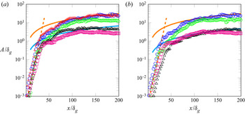
In figure 14, we present the effect of confinement on wave amplitude. We start by studying in figure 14(a) the effect of a reduction of  $H$ for a symmetric confinement, from
 $H=2$ cm (
 $+$, red) to
 $H=0.15$ cm (
 $\square$, magenta). One can see that the reduction of
 $H$ induces a global decrease of the amplitude in the downstream region. The growth close to the inlet, i.e.
 $x/\delta _g \le 25$, does not seem to be affected until the amplitude is of the order of the gas vorticity thickness. Farther downstream, the lower the value of
 $H$, the earlier the amplitude seems to depart from the self-similar growth model, and stabilize up to a constant value increasing with
 $H$.
Effect of confinement on the amplitude for case B2 with  $n=2$. (a) Effect of the reduction of
 $H$ for a symmetric confinement (
 $H_g=H_l=H$):
 $H=2$ cm (+, red);
 $H=1$ cm (
 $\circ$, blue);
 $H=0.5$ cm (
 $\circ$, green);
 $H=0.25$ cm (
 $\triangle$, black);
 $H=0.15$ cm (
 $\square$, magenta). (b) Evidence of the non-symmetric effect of the gas and liquid thicknesses on the amplitude:
 $H_l=H_g=1$ cm (
 $\circ$, blue);
 $H_g=0.15$ cm and
 $H_l=1$ cm (
 $\circ$, green);
 $H_l=0.15$ cm and
 $H_g=1$ cm (
 $\triangle$, black);
 $H_l=H_g=0.15$ cm (
 $\square$, magenta). In both plots, only one data point in every four is shown to enhance readability. Here (4.1), with
 $A_0/\delta _g=0.0003$ and
 $k_i=614.6$ m
 $^{-1}$ (orange dashed line); (4.2), with
 $C_0=0.21$ (Orange solid line); (4.2), with (a):
 $C_0=0.045$, and (b):
 $C_0=0.032$ (Cyan solid line).

To clarify the effect of each stream thickness on the wave amplitude, we present in figure 14(b) the effect of a reduction of  $H_g$ only (
 $\circ$, green),
 $H_l$ only (
 $\triangle$, black) and both (
 $\square$, magenta). One can see that, although the effect of both stream thicknesses on the frequency is symmetric, the effect on the amplitude is non-symmetric. It seems that the decrease in amplitude observed in figure 14(a) between
 $H=2$ cm (symbol
 $+$, red) and
 $H=0.15$ cm (symbol
 $\square$, magenta) is mainly due to the decrease of
 $H_l$ since the same decrease is observed when only
 $H_l$ is reduced (symbol
 $\triangle$, black in figure 14b). It also seems that when
 $H_l$ only is reduced, the growth is slower in the region close to the injector, which agrees with the experimental observations of Marty (Reference Marty2015).
Similarly, the departure from the self-similar model seems to be due to the reduction of  $H_g$. Following the derivation of the self-similar model in Hoepffner et al. (Reference Hoepffner, Blumenthal and Zaleski2011), the amplitude increase in the nonlinear area is due to the aerodynamic suction created by the acceleration in the gas stream when deviated by the wave. When the wave amplitude becomes large compared with the gas stream, there is no longer a sufficient acceleration to induce wave growth.
5.3. Scaling law for confinement modes
The destabilizing effect of confinement has been demonstrated and explored by means of numerical simulations and linear stability analysis in previous subsections. In Matas et al. (Reference Matas, Delon and Cartellier2018), a scaling law derived from the linearized equations was proposed for the wave frequency in confinement-induced absolute modes,
 \begin{equation} f \sim \frac{\sqrt{\dfrac{\rho_g}{\rho_l}\dfrac{\delta_l}{\delta_g}}U_g+U_l}{L}, \end{equation}
where  $L$ is a characteristic length related to the confinement. This scaling has recently been found to account very well for the effect of the nozzle size in experiments on a coaxial configuration (Singh et al. Reference Singh, Kourmatzis, Gutteridge and Masri2020). Equation (5.1) predicts a linear evolution of the frequency with the liquid velocity, which has been observed experimentally (Matas et al. Reference Matas, Marty and Cartellier2011; Singh et al. Reference Singh, Kourmatzis, Gutteridge and Masri2020). In the case of large gas velocity,
 $\delta _g \ll \delta _l$, and for
 $\delta _g$ varying as
 $U_g^{-1/2}$, the frequency is proportional to
 $U_g^{5/4}$, which is close to the scaling predicted by inviscid theory (Raynal Reference Raynal1997; Marmottant & Villermaux Reference Marmottant and Villermaux2004), see § 1. Note that the scaling of (5.1) is only valid for absolute modes due to confinement.
In order to compare our results to the scaling of (5.1), we add lines enhancing the scaling of the frequency with  $H$ in absolute regimes in figure 12. In the confinement-induced absolute regime, we find that the most amplified frequency follows a
 ${\sim }1/H$ scaling in the case of symmetric confinement. For
 $H_g \ne H_l$, as seen in figure 13, it seems that the frequency scales with the most restrictive confining length, i.e.
 \begin{equation} f \sim 1/\min(H_g,H_l). \end{equation}
Thus, our results match very well with the scaling of (5.1) and we evidence that  $L$ is of the order of the smallest injector size. This is different from what has been observed experimentally by Delon, Cartellier & Matas (Reference Delon, Cartellier and Matas2018) for a coaxial geometry, where the frequency is found to always scale with
 $1/H_l$. The shear branch being barely affected by the value of
 $H$, frequency is expected to be independent of the confining size in the convective regime.
6. Conclusion
The confinement of the air–water mixing layer has previously been found to be the missing element allowing us to reconcile experimental wave frequencies with viscous linear theory. In this paper, we have shown for the first time the convergence between linear theory, experiments and numerical simulations on the values of the wave frequency, in regimes where the absolute instability is predicted to be due to confinement. We have shown that, in those conditions, waves are self-similar in the downstream area following the model of Hoepffner et al. (Reference Hoepffner, Blumenthal and Zaleski2011). We proved that the confinement is indeed a mechanism for the transition between convective and absolute regimes and described precisely the characteristics of the instability in both regimes. The gas and liquid streams thicknesses are found to have symmetric effects on wave frequency, as first suggested in Matas (Reference Matas2015), but not on the wave amplitude. A symmetric confinement and a high dynamic pressure ratio can favour the triggering of an absolute instability, hence enlarging the range of validity of the scaling law given in (5.1). Finally, it seems that the most amplified frequency scales with the most restrictive confining length, i.e. the thinnest stream, in the absolute regime, which is different from what has been observed on a coaxial configuration.
Note that the characteristics of confinement modes presented in § 5.1 (large wavelength of the order of, or larger than injector size, and wave speed close to Dimotakis’) have also been found in moderate density ratio simulations (Jiang & Ling Reference Jiang and Ling2021), which suggests that the results of the present paper may apply to a wide range of injection conditions.
These conclusions only focus on the transition between convective and confinement- induced absolute regimes. As shown in Otto et al. (Reference Otto, Rossi and Boeck2013), Fuster et al. (Reference Fuster, Matas, Marty, Popinet, Hoepffner, Cartellier and Zaleski2013) and Matas et al. (Reference Matas, Delon and Cartellier2018), a surface tension-induced absolute regime is dominant as soon as the interfacial wave speed is low enough so that capillary waves are able to send information upstream. This transition is driven by  $\delta _d$, the deficit parameter, and in fine by the presence of the splitter plate between gas and liquid streams. The configuration we chose to simulate would allow a precise study of the impact of
 $\delta _d$ on the instability and on the flow statistics. This task would be an essential step to understand how the spatial development of the flow affects the instability regime, through the selection of
 $\delta _d$. However, we have shown that this is a very expensive task, even in two dimensions, that we leave for future work. Our results also suggest that the use of fine meshes in 2-D simulations can give rise to some unphysical effects due to 2-D turbulence. A 3-D mesh convergence would be needed to study spatial frequency variations and to study the global, or not, nature of the instability, but this, again, is an highly expensive task that we leave for future work.
Acknowledgements
C.B. is grateful to Dr R. Chiodi for many discussions about the simulation of an air–water mixing layer.
Funding
This work was sponsored by the Office of Naval Research (ONR) as part of the Multidisciplinary University Research Initiatives (MURI) Program, under grant number N00014-16-1-2617, and by the IDEX UGA ‘International Strategic Partnerships’ program. A part of the simulations were performed using HPC resources from GENCI-CINES (grant no. A0072A00611).
Declaration of interests
The authors report no conflict of interest.