1. INTRODUCTION
Maritime traffic levels are related to economic growth: the international shipping industry is responsible for delivering about 90% of all trade worldwide by volume (with 7 to 9 billion tons loaded per year), and it is vital for bulk transport of raw materials, oil and gas. The linear regression between the economic growth of the nations in the Organisation for Economic Cooperation and Development (OECD) shows a 4% increase of imports and exports for a 1% increase in Gross Domestic Product (GDP). So, marine transportation is an integral, although sometimes less visible, part of the global economy. Other important marine activities include passenger transportation (ferries and cruise ships), national defence and fishing. If we also consider pleasure boats, even forgetting the millions of smaller leisure boats worldwide, the spatial density of marine traffic increases significantly, especially in areas close to harbours and coasts.
To improve the safety and the efficiency of marine traffic, as well as to protect the environment, Vessel Traffic Service (VTS) definitions and regulations were introduced by the International Maritime Organization (IMO) in 1985 and then updated in 1997 with the Resolution A.857(20) (IMO, 1997). VTS makes use, among other sensors, of powerful coastal radars to obtain an up-to-date marine traffic image. Vessels themselves can carry radars for navigation purposes. For decades these navigation radars have been designed as cheap pulsed magnetron devices emitting very short (e.g. less than 10−1 μ s) pulses with high peak power of the order of tens of kW. More recently, new solid-state technology has entered marine radar design (Zhang et al., Reference Zhang, Dong and Liu2013; Amato et al., Reference Amato, Fiorini, Gallone and Golino2010; Nelander and Tòth-Pàl, Reference Nelander and Tòth-Pàl2009). With a solid-state power amplifier, marine radars are becoming more and more sophisticated and agile in frequency as well as in waveform in order to get better performance by pulse compression, all features that were not possible with the old magnetron transmitter. Since the solid-state amplifiers' power is of the order of tens of W, significantly less than magnetrons', they have to transmit longer pulses (e.g. up to 90–100 μ s) in order to achieve the same energy on target, i.e. keep the detection probability unchanged with respect to magnetron radars. Their longer pulses cause a time-domain overlapping (interference) of several returns belonging to different radars, that is to different vessels. The main factors that affect interference between radars are: frequency, pulse rate, rotation rate and distance. The time-domain asynchronous interference in the older magnetron radar can be treated using simple Interference Rejection (IR) techniques. With the “long pulse” of solid state radars, the interference problem is much more marked and calls for a more complex interference mitigation technique (Galati et al., Reference Galati, Pavan and De Palo2015). The various above-mentioned factors are included in a mathematical model which is fully described in Galati et al. (Reference Galati, Pavan and De Palo2016).
In this paper we focus on the distance between radars. Using real-world AIS data for the Mediterranean Sea, a statistical model of the mutual distances between vessels has been evaluated. By this it is possible to estimate the mean number of nearby ships in radar range, where the visibility depends on the radar antennae's heights.
The problem of knowing the statistical mutual distance distribution between vessels has not been addressed in literature so far. Rather, the typically addressed problem is the modelling of vessel traffic by means of fuel savings and flow prediction through both neural networks (Haiyan and Youzhen, Reference Haiyan and Youzhen2015) and weighted graphs (Hang et al., Reference Hang, Xu, Chen and Zhou2015). Image processing techniques have also been used for marine traffic applications, although most aimed to detect anomalies (Kraiman et al., Reference Kraiman, Arouh, Webb, Sisti and Trevisani2001; Riveiro, Reference Riveiro2011) or vessel movements (Willems et al., Reference Willems, Wetering and Wijk2009). Other works are related to high-risk spot identification from an AIS reports database (Chang et al., Reference Chang, Hsu, Yang, Chen, Chiu and Chang2010) as well as to traffic flow composition and vessel arrival or passage time. Within this paper we do not need to take account of the time parameter since the main goal is the evaluation, at a given time, of the mean number of nearby vessels. Of course this number depends on temporal traffic flow evolution but, from a radar design point of view, only the maximum value is significant, i.e. the value related to the time instant with the maximum number of sailing vessels.
Knowing the mutual distance distribution will also lead to a kind of marine traffic topology classification, i.e. to decide whether ships, at a given time, are following a route or whether they are “randomly” sailing over a finite region. An interesting related work by Su and Chang (Reference Su and Chang2008) aimed at detecting the presence of fishing vessel spatial clusters for over-fishing prevention. The added value of the mutual distance approach is the detection of routes in addition to the distributed clusters.
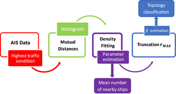
The main goal of this paper is to classify traffic topology by using a single statistical parameter estimated from the observed real-world AIS data. Figure 1 presents the workflow chart of the proposed statistical approach.
Workflow chart: from the AIS data to the traffic topology classification.

Starting from the full AIS reports database, the mean number of nearby ships is obtained, finally the traffic topology is classified through a single parameter (β) estimation.
In Section 2 AIS data is shown with the related statistical analysis in which the parameters of the Gamma and Generalised Gamma models are estimated. Section 3 considers the truncation of the statistical distribution of the mutual distances in order to evaluate the mean number of ships in a given region. The relationship between the statistical model parameters and the topology of the traffic has been investigated. In the Appendix a more general theoretical Poisson-like model is described for the sake of comparison. Note that all distances are in nautical miles (NM).
2. THE MARINE TRAFFIC MODEL
In this section the statistical model for the mutual distances is derived from AIS data.
2.1. AIS data and their distribution
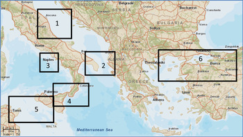
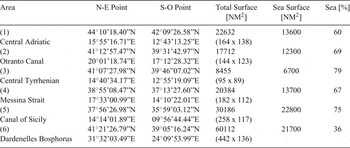
The General Command of the Italian Coast Guard kindly provided the AIS data for the week 23 February – 1 March 2015 related to six areas: (1) Central Adriatic, (2) Otranto Canal, (3) Central Tyrrhenian, (4) Messina Strait, (5) Canal of Sicily and (6) Dardanelles/Bosphorus (see Figure 2 and Table (1a) for more details).
View of the six Mediterranean areas.

Main characteristics of the six areas.

Each area was originally sampled at a rate of one minute, then the huge AIS reports database has been reduced to a rate of four hours from midnight. We have taken the four-hour interval in which maximum traffic appears, neglecting what happens in each other four-hour time period. From data inspection, however, we did not perceive a significant deviation from the maximum traffic situation within the interval, so our analysis is conservative (Galati et al., Reference Galati, Pavan and De Palo2015; Galati and Pavan, Reference Galati and Pavan2015).
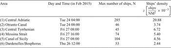
From the first analysis of the AIS data, we derived the time interval having the maximum number of ships in each area, as shown in Table (1b). In the following we refer to the area with the highest traffic as the area with the highest number of ships. The density z [ships/NM2] of en-route ships is computed as the number of ships over the sea surface (Table (1a)) in the highest traffic condition. We extrapolated the position of ships from the AIS data related to Table (1b) (i.e. highest traffic condition) for each area. We used the flat earth approximation for distance due to the small-sized areas (max distance in area (6) is about 370 NM).
Maximum number of ships per each area and their density z. Data for the week 23 February - 1 March 2015.

The number of mutual distances is:
 $$N=\displaystyle{{n\cdot \lpar n-1\rpar } \over{2}} $$
in which n is the total number of ships in the area in a given time interval (e.g. with the highest traffic condition). It is worth noting that the N distances are not statistically independent because they are among ships: given n ships, if only one of them is moved, n − 1 distances do change.
2.2. Statistical analysis of inter-ship distances
The ship-to-ship distance R can be fitted with a probability density function f
R
(r) having the following properties: f
R
(r) = 0 for r ≤ 0 and
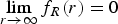 $\lim_{r\to\infty} f_{R}\lpar r\rpar =0$
.
A suitable candidate for this positive random variable is the Gamma model (Papoulis, Reference Papoulis1990) defined by two parameters (i.e. the scale parameter λ and the shape parameter b):
 $$f_{R}\lpar r\rpar =\displaystyle{{\lambda^{b}}\over{\Gamma \lpar b\rpar }}r^{b-1}e^{-\lambda r}\ r\ge 0 $$
where
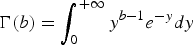 $\Gamma \lpar b\rpar =\vint_{0}^{+\infty } y^{b-1}e^{-y}dy$
is the Gamma function. To improve the model, a third parameter μ can be added into Equation (2) obtaining a Generalised Gamma model (Stacy, Reference Stacy1962):
 $$f_{R}^{GEN}\lpar r\rpar =\displaystyle{{\mu \cdot \lambda^{b\mu }}\over{\Gamma \lpar b\rpar }} r^{b\mu -1}e^{-\lpar \lambda r\rpar ^{\mu}}\ r\ge 0 $$
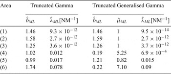
When μ = 1 the Generalised Gamma density function equals the Gamma model. These parameters can be estimated by the Maximum Likelihood (ML) method, which leads to a system of non-linear equations whose solutions are the values in Table (2a) and Table (2b), where the estimated mean values
 ${\hat m}_R$
(in NM) are shown.
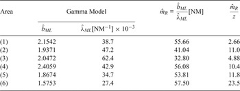
Estimated parameters of the Gamma model for the six areas.

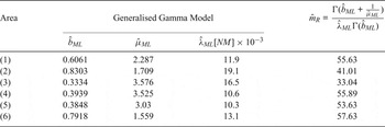
Estimated parameters of the Generalised Gamma model for the six areas.

The sample size for each area varies from 990 distances with average value of 32.80 NM (Area 3) to 40,470 distances with average value of 55.66 NM (Area 1). Day and time are listed in Table (1b). For the Gamma model the ratio
 $\displaystyle{{\hat{m}_{R}}\over{z}} \lsqb \displaystyle{{\hbox{NM}^{3}}\over{ships}}\rsqb $
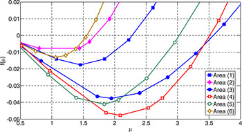
gives an idea about the topology of the traffic on the considered sea surface (e.g. en-route or randomly distributed): low ratio values correspond to a distributed, or random, topology (i.e. Central Adriatic, Area (1)), while higher values are related to a route or more regular topology (for example, in Otranto Canal (2), Messina Strait (4) and Canal of Sicily (5)). Moreover, we observe that the ML estimation of μ leads to a system of three non-linear equations where the μ-th power of the sample values (i.e. the measured distances) is present. Therefore, it is necessary to find that value of μ whereby the derivative of the Likelihood function, f(μ), is equal to zero (see Figure 3). However, as shown in Figure 3, the values of f(μ) in the range of practical interest, i.e. 0 < μ< 3, are close to zero, i.e. there are sub-optimal solutions (values of μ̂) that can be considered, including μ̂ = 1. The use of μ̂ = 1 simplifies the model leading back to the Gamma model that looks more convenient than its generalisation (see also in the following).
The derivative of the Likelihood function for the estimation of the Generalised Gamma parameter μ. The μ̂ ML is obtained posing f(μ) = 0.

To validate the estimated parameters
 $\hat{b}_{ML}\comma \; \hat{\mu }_{ML}\comma \; \hat{\lambda}_{ML}$
the Kolmogorov-Smirnov test and the χ2 test (Papoulis Reference Papoulis1990) should be applied with the null hypothesis being (respectively for the Gamma and the Generalised Gamma distribution):
 $H_{0}\colon F\lpar r\rpar =F_{R}\lpar r\rpar $
or
 $H_{0}\colon F\lpar r\rpar =F_{R}^{GEN}\lpar r\rpar $
. However, since the N distances are not statistically independent, the tests too often reject the null hypothesis H
0 (Gleser and Moore, Reference Gleser and Moore1983), and cannot be effectively applied in the present case. However, a visual inspection gives a fairly good idea of the goodness of fit of the measured mutual distances with these distributions.
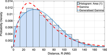
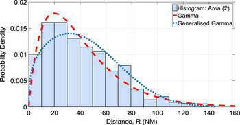
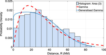
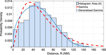
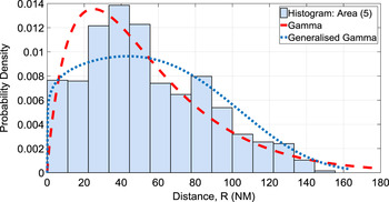
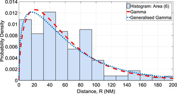
In Figures 4(a)–(4(f)) the histograms of distances for all areas are presented with the overlapped Gamma and Generalised Gamma estimated models. In some cases, e.g. Areas (3) and (5), the Generalised Gamma model is not the best fit because the third parameter μ improves the fit only locally. Hence, a first result of this study is that when considering the ship-to-ship distances a three parameters distribution such as the Generalised Gamma does not practically improve the goodness of fit with respect to a simpler, straightforward distribution such as the Gamma. Therefore, the Gamma model with parameters λ and b will be used in this work.
Histogram and densities of R for Area (1).

Histogram and densities of R for Area (2).

Histogram and densities of R for Area (3).

Histogram and densities of R for Area (4).

Histogram and densities of R for Area (5).

Histogram and densities of R for Area (6).

3. VISIBILITY
In the previous section we have shown that the distances between pairs of ships can be represented by a random variable R distributed according to a Gamma model with parameters b and λ.
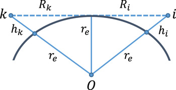
As explained before, it is useful to consider, for a generic ship, the mean number of vessels in its surroundings within a specific area (Galati et al., Reference Galati, Pavan and De Palo2015). The radar horizon – with the 4/3 earth propagation model – and the heights of ships must be considered to compute the maximum distance at which two on board radars may interfere. Radar horizon for two ships labelled “i” and “k” is related to the heights of on board radars h k and h i (see Figure 5).
Radar horizon between ships k and i.

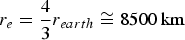
In the standard atmosphere, making use of the equivalent earth radius
 $r_{e}=\displaystyle{{4}\over{3}}r_{earth}\cong 8500\, \hbox{km}$
, the horizon R
ki
is:
 $$R_{ki}=R_{k}+R_{i}\cong \sqrt {2r}_{e} \cdot \lpar \sqrt h_{k} +\sqrt h_{i}\rpar $$
The antenna height, not being included in AIS data, must be estimated. Based on the AIS information of the ship and on photos of the various types of ship, we have empirically estimated the relationship between the length (as provided by AIS) of the ship and the radar antennae height (Galati et al., Reference Galati, Pavan and De Palo2015). For example, if we consider two cargo ships with their radar antennae at 30 m above sea level, the optical horizon is about r MAX = 35 NM, while it becomes r MAX = 10 NM for small and pleasure boats, because of the antenna heights of the order of 4 m. In this section we focus only on the latter case (r MAX = 10 NM). Let us consider an all-sea circular section with diameter r MAX . It is possible to calculate the average number of ships (randomly) distributed in this circular sea surface through the probability P that the mutual distances do not exceed r MAX :
 $$P\lcub R\le r_{MAX}\rcub =\displaystyle{{1}\over{\Gamma\lpar b\rpar }}\vint_0^x {e^{-t}t^{b-1}dt} =\gamma \lpar b\comma \; x\rpar $$
where γ (b, x) is the Incomplete Gamma Function (Abramowitz and Stegun, Reference Abramowitz and Stegun1964) with
 $x=\lambda \cdot r_{MAX}$
. The parameters b and λ have been estimated with the Maximum Likelihood method for each area (Tables (2a) and 2(b)). Multiplying the probability in Equation (5) by the total number of ships in the area (n
TOT
) we obtain the expected number of ships inside this circular sea surface:
 $$n_{ships}=P\lcub R\le r_{MAX}\rcub \cdot n_{TOT} $$
The probability density of the random variable R, i.e. the mutual distances among the n
ships
vessels in the area (with
 $0\le R\le r_{MAX}$
) is given by the conditional density function of Equation (2):
 $$f_{R}\lpar r\vert R\le r_{MAX}\rpar = \left\{\matrix{\displaystyle{{f_{R}\lpar r\rpar }\over{F_{R}\lpar r_{MAX}\rpar }} & 0\lt r\lt r_{MAX} \hfill \cr 0 & r\ge r_{MAX} \hfill \cr}\right. $$
This approach would use the same parameters as estimated for the original model and therefore might not be fully reliable. Using Equation (7) to compute the conditional density model from the Gamma model with parameters b, λ we can readily obtain:
 $$f_{R}\lpar r\vert R\le r_{MAX}\rpar = \left\{\matrix{\displaystyle{{\lambda^{b}x^{b-1}e^{-\lambda x}}\over{\gamma \lpar b\comma \; \lambda r_{MAX}\rpar }} & 0 \lt r \lt r_{MAX} \hfill \cr 0 & r \ge r_{MAX} \hfill \cr} \right. $$
In Equation (8) we have added the third parameter r MAX named “truncation parameter” which takes into account the maximum distance at which the model should be considered (e.g. the optical horizon).
To estimate b and λ in Equation (8), having fixed the value of r MAX , a closed-form solution such as the well-known one for the Gamma and Generalised Gamma distributions does not exist. The problem of finding the maximum for the Likelihood function must be solved by a non-linear optimisation method. We have used the Nelder-Mead algorithm (Nelder and Mead Reference Nelder and Mead1965). This estimation often gives very low values for λ, as shown in Table 3 for Areas (1) – (4).
Estimation of b, μ, λ for r MAX =10 NM.

For this reason a different model, when λ → 0, has been considered for the short range distance between a pair of vessels, i.e. r < r MAX , having set r MAX = 10 NM.
3.1. Short Range Model
In Equation (8) when λ is close to zero, the only significant remaining term is x b−1 multiplied by a constant c depending on b. Posing β = b − 1 we obtain:
 $$f_{R}\lpar r\vert R\le r_{MAX}\rpar =c\cdot x^{\beta }\quad 0 \lt r \lt r_{MAX} $$
The unity area condition for Equation (9) leads to:
 $$c=\displaystyle{{\beta +1} \over{r_{MAX}^{\beta +1}}} $$
Therefore, the conditional density for truncated distances with a single parameter β is:
 $$f_{R}\lpar r\vert R\le r_{MAX}\rpar = \left\{\matrix{\displaystyle{{\beta +1}\over{r_{MAX}^{\beta +1}}}\cdot r^{\beta } & 0 \lt r \lt r_{MAX} \hfill \cr 0 & r\ge r_{MAX} \hfill \cr}\right. $$
Normalising with respect to r
MAX
, i.e. posing
 $\hat{r}=\displaystyle{{r} \over{r_{MAX}}}$
in Equation (11) and multiplying Equation (11) for r
MAX
, results in:
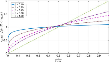
 $$r_{MAX}\cdot f_{R}\lpar r \vert R\le r_{MAX}\rpar =\left\{\matrix{\lpar \beta+1\rpar \cdot \hat{r}^\beta & 0 \lt \hat{r} \lt 1 \hfill \cr 0 & r \ge 1 \hfill \cr}\right.$$
Figure 6 shows Equation (12) for different values of β (0 < β≤ 1). If λ → 0 (see Table 3) the Gamma model leads to Equation (11) and if β → 0 the model converges to the uniform model:
 $$f_{R}\lpar r \vert R\le r_{MAX}\rpar =\displaystyle{{1}\over{r_{MAX}}}\quad 0 \lt r \lt r_{MAX} $$
Normalised conditioned density model.

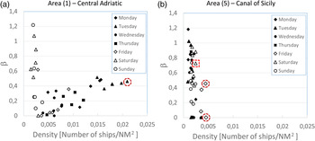
In the following, we show the results related to Central Adriatic, Canal of Sicily and Strait of Messina. It is known that the traffic in the Central Adriatic is mainly due to fishing boats whose positions include a large number of randomly distributed clusters. In the Canal of Sicily the vessel traffic can be classified as traffic near the coast (where normally fishing boats are the majority with some possible localised clusters) and traffic along the sea routes where cargo ships, container ships and tankers prevail. The difference in ship type leads us to evaluate the r MAX limit: the bigger the ship, very likely the higher is its radar antenna, and so the wider is its interference area. Figure 7(a) and (b) show the estimated values of β using all data during the week 23 February – 1 March 2015 (42 values in total) versus the ship's density (number of ships per unit area) for Area (1) and Area (5) respectively.
Estimated values of: (a) Area (1); (b) Area (5).

From Figures 7(a) and 7(b) we can deduce the following:
-
(i) If the density of ships is much lower than 2.5 × 10⁻³ ships/NM2 (in Central Adriatic it occurs mostly during the weekend when the fishery is strongly reduced), the low number of samples does not allow us to estimate β correctly.
-
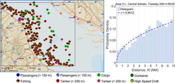
(ii) For Area (1) increasing the density, i.e. when the density is greater than 2.5 × 10⁻³ ships/NM2, the estimated β increases to around 0.5. For the maximum density of 20.88 × 10⁻³ ships/NM2, β is 0.461 (dashed circle in Figure 7(a)); this case corresponds to the traffic shown in Figure 8 where the scenario is shown on the left (251 fishing boats and 33 other vessels). On the right the estimated truncated density function is plotted. The latter agrees with the data (see histogram).
-
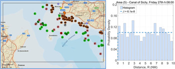
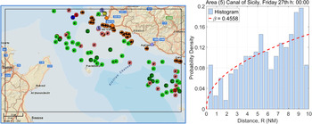
(iii) For Area (5) the density always remains below 5 × 10⁻³ ships/NM2. Considering the two higher observed densities, i.e. 4.56 × 10⁻³ and 4.47 × 10⁻³ ships/NM2, corresponding to the traffic shown in Figures 9(a) and 9(b) respectively, the estimated β is 6.1 × 10⁻⁸ and 0.4558 (dashed circles in Figure 7(b)). The different conditioned distribution is due to the fact that in the first case (h: 08:00), in comparison with the second one (h: 00:00), the presence of a greater number of fishing vessels (close to each other) implies an increase of the short ranges into the interval (0, r MAX = 10 NM). In the second case the decrease of fishing boats in a few localised clusters and the increase of the others (cargo ships, container ships and tanks) cause an increase of the higher ranges as shown in Figure 9(b).
Scenario of traffic for Area (1) Central Adriatic, Tuesday 24 at 08:00 and the estimated truncated density function. Fishing boats: 251 (88 %), others: 33 (12 %).

Distributed traffic of Area (5) Canal of Sicily, Friday 27 at 08:00 and estimated truncated density function. Fishing boats: 62 (60%), others: 42 (40%).

Distributed traffic of Area (5) Canal of Sicily, Friday 27 at 00:00 and estimated truncated density function. Fishing boats: 31 (30%), others: 71 (70%).

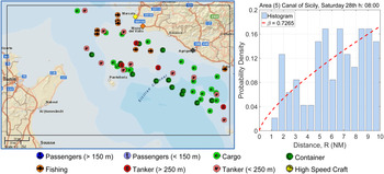
For the Canal of Sicily, a third case (Saturday 28 at 08:00) is shown in Figure 9(c) when cargo ships, container ships and tankers are predominant in comparison with the fishing boats. The density of ships is low, z = 2.46× 10⁻³ ships/NM2, and no clusters of fishing vessels are present. The other vessels, i.e. cargo ships, container ships and tankers, are more uniformly distributed along the routes. The resulting value of β = 0.7265.
Distributed traffic of Area (5) Canal of Sicily, Saturday 28 at 08:00 and estimated truncated density function. Fishing boats: 8 (14%), others: 48 (86%).

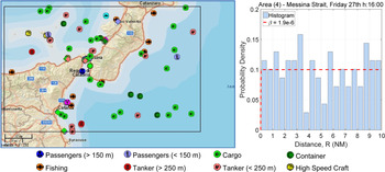
The traffic in the Strait of Messina (Friday 27 at 16:00) is shown in Figure 10, where it is mainly due to large vessels and no localized clusters of fishing boats are present. The parameter β resulting is close to zero.
Distributed traffic of Area (4) Messina Strait, Friday 27 at 16:00 and estimated truncated density function. Fishing boats: 9 (12%), others: 65 (88%).

Table 4 reports the ML estimate of β for the six marine areas considering the maximum observed density of ships for each area with r MAX = 10 NM.
Maximum Likelihood Estimate of β with r MAX =10 NM.

From Table 4 we can find very low values for β in Areas (4) and (5). It is worth noting that in Area (6) β is comparable with that in the Central Adriatic although the area provides a main route. This effect is due to the presence, in Area (6), of two different seas (Aegean Sea and Sea of Marmara) as well as of the Dardanelles, one of the world's narrowest straits used for international navigation, with the likely effect of strongly distorting the behaviour of ships' distances with respect to the open sea. In general, the sea percentage in Table 1 also gives an idea about the reliability of the β values.
From the previous results we can maintain that when the density of ships is high enough to validate the results, the values of β are strongly dependent on the topology of the observed traffic and on the geographic area: β close to 0.5 represents many clusters of ships uniformly distributed over the sea, mainly due to small boats near to the coast (fishing boats). Values of β close to zero denote the absence of groupings of small boats, i.e. in this case large vessels are present away from the coast along the routes. Special evaluations should be done near harbours or close to the straits as they occur near Messina or in the Dardanelles areas.
In the Appendix, for comparison, a mathematical model is shown, based on a general bi-dimensional Poisson model. However, the use of the model is limited by the conditions of the real scenario that imposes a different topology of traffic (near to and far from the coast) that are non-uniformly distributed over the sea and, sometimes, strong limitations due to the geography of the area (presence of coasts, islands, straits, canals and harbours).
4. CONCLUSIONS
A full AIS report database has been provided by the Italian Coast Guard for six marine areas of the Mediterranean Sea. The sampled real-world AIS data have been used to create a statistical model for vessel-to-vessel mutual distances. A Gamma distribution fits the empirical vessel-to-vessel mutual distances well while the more complicated Generalised Gamma distribution does not improve the goodness of fit.
The need to know the mutual distance distribution arises due to the advent of the new solid state pulse compression marine radars whose operation is based on long pulses that are very likely to time-overlap each other. One promising radar interference rejection technique exploits the matched filter's pulse compression and provides for the transmission of several orthogonal radar signals, one for each radar. The number of needed orthogonal signals must be evaluated according to the number of nearby interfering ships. The statistical distribution of the mutual distances allows us to find it provided the area is limited to a maximum value r MAX , which in turn is related to the ships' type size which is strongly correlated to the radar antenna height. The higher the radar antenna, the wider the interference area r MAX , the higher the number of interfering vessels. In this paper we have mostly focused on the small to medium vessels with r MAX = 10 NM.
By truncating the mutual distances distribution to r MAX it is possible to get a type of traffic topology classification which is easily handled by the single parameter β. The said classification is aimed to qualitatively evaluate the way in which the ships are positioned at a given time, whether randomly distributed (e.g. β ≈ 0) or in a line (e.g. β → 1) following some route.
From a more theoretical point of view, a mathematical approach based on the 2D Poisson points model leads to a more complex, polynomial truncated density function which, for a truncation distance much less than the dimension of the marine area, converges to a triangular density function, i.e. the same as the empirical model with β = 1.
More generally, the model is not aimed to predict any marine traffic behaviour, nor to optimise routes and fuel consumption.
The presented work is preliminary. The found model might lead to a powerful analysis of marine radar interferences from a statistical point of view, also leading to a change in solid state radar design starting from the proposed use of the orthogonal signals as a possible interference rejection technique. Moreover, other significant case studies may be analysed to prevent the model being affected by a particular coast's morphology or fishing vessel behaviour.
ACKNOWLEDGEMENTS
Special thanks are due to the Italian Coast Guard for kindly providing AIS traffic data.
APPENDIX. GENERAL POISSON MODEL
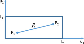
A possible mathematical model for the distribution of ships in marine traffic can start from the bi-dimensional points of Poisson inside a rectangle. It supposes that the ships are uniformly placed over the sea within a rectangle. Let us consider a rectangle with sides L 1 and L2 (L2 < L1) and a pair of random points (P 1, P 2) inside it (see Figure A1). It is supposed that the coordinates (U 1, U 2) of each point P i are uniformly distributed in (0, L 1) and (0, L 2) respectively.
Two random points inside the rectangle (L 2 < L 1).

Then the distance
 $R=\overline {P_{1}P_{2}} $
has a probability density function given by (Philip, Reference Philip1991):
 $$f_{R}\lpar r\rpar =\displaystyle{{2\pi r}\over{L_{1}L_{2}}}-\displaystyle{{4r^{2}}\over{L_{1}L_{2}^{2}}}-\displaystyle{{4r^{2}}\over{{L_{1}^{2}L}_{2}}}+\displaystyle{{2r^{3}}\over{L_{1}^{2}L_{2}^{2}}}\quad 0 \lt r \le L_{2} $$
 $$f_{R}\lpar r\rpar =-\displaystyle{{2r}\over{L_{1}^{2}}}-\displaystyle{{4r^{2}}\over{L_{1}L_{2}^{2}}}+\displaystyle{{4r}\over{L_{1}L_{2}}} arcsin\left(\displaystyle{{L_{2}}\over{r}}\right)+\displaystyle{{4r}\over{L_{1}L_{2}^{2}}}\sqrt {r^{2}-L_{2}^{2}} \quad L_{2} \lt r\le L_{1}$$
 $$\eqalign{f_{R}\lpar r\rpar &= -2r\left[\displaystyle{{1}\over{L_{1}^{2}}}+\displaystyle{{1}\over{L_{2}^{2}}}\right]+\displaystyle{{4r}\over{L_{1}L_{2}}}\left[arcsin\left(\displaystyle{{L_{1}}\over{r}}\right)+arcsin\left(\displaystyle{{L_{2}}\over{r}} \right)\right]\cr & \quad +\displaystyle{{4r}\over{L_{1}L_{2}}}\left[\sqrt {\left(\displaystyle{{r}\over{L_{1}}}\right)^{2}-1} +\sqrt {\left(\displaystyle{{r}\over{L_{2}}} \right)^{2}-1} \right]-\displaystyle{{2\pi r}\over{L_{1}L_{2}}}-\displaystyle{{2r^{3}}\over{L_{1}^{2}L_{2}^{2}}} \cr & \qquad L_{1} \lt r\le \sqrt {L_{1}^{2}+L_{2}^{2}}}$$
 $$f_{R}\lpar r\rpar = 0 \qquad elsewhere $$
Without loss of generality we pose L 1 = cL 2 with the constant c ≥ 1.
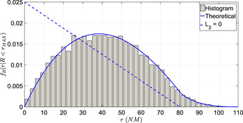
For c = 1 and c = 20 the density functions f R (r) are shown in Figures A2(a) and A2(b) respectively (continuous line).
Density function of R for c = 1 (L 1 = L 2 = 80 NM).

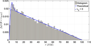
Density function of R for c = 20 (L 1 = 100 NM, L 2 = 5 NM).

When L 2≪L 1 (at limit L 2 → 0 with a finite value of L 1) the density f R (r) converges to a triangular shape (dashed line). In Figures A2(a) and A2(b) the histograms of data (obtained by simulation, i.e. randomly allocating a large number of vessels in the rectangular area (12,686 for Figure A2(a) and 12,294 for Figure A2(b)) and measuring their mutual distances) are also shown.
For 0 < r ≤ L 2 the density f R (r) can be rewritten as:
 $$f_{R}\lpar r\rpar =\displaystyle{{2\pi r}\over{cL_{2}^{2}}}-\displaystyle{{4r^{2}}\over{cL_{2}^{3}}} -\displaystyle{{4r^{2}}\over{c^{2}L_{2}^{3}}}+\displaystyle{{2r^{3}}\over{c^{2}L_{2}^{4}}}\quad 0 \lt r\le L_{2} $$
and the corresponding distribution function in the interval (0, L 2) is:
 $$F_{R}\lpar r\rpar =\displaystyle{{\pi r^{2}}\over{cL_{2}^{2}}}-\displaystyle{{4r^{3}}\over{3cL_{2}^{3}}} -\displaystyle{{4r^{3}}\over{{3c}^{2}L_{2}^{3}}}+\displaystyle{{r^{4}}\over{{2c}^{2}L_{2}^{4}}} \quad 0\lt r\le L_{2} $$
If we suppose r MAX ≤ L 2, the conditioned density to the event {R < r MAX } results:
 $$f_{R}\lpar r\vert R< r_{MAX}\rpar =\displaystyle{{f_{R}\lpar r\rpar }\over{F_{R}\lpar r_{MAX}\rpar }}\quad 0\lt r\le r_{MAX} $$
Substituting Equations (A5) and (A6) we obtain:
 $$f_{R}\lpar r\vert R \lt r_{MAX}\rpar = \left\{\matrix{\displaystyle{{2\pi r-\displaystyle{{4r^{2}}\over{L_{2}}}\left(1+\displaystyle{{1}\over{c}} \right)+\displaystyle{{2r^{3}}\over{cL_{2}^{2}}}}\over{\pi r_{MAX}^{2}-\displaystyle{{4r_{MAX}^{3}}\over{3L_{2}}}\left(1+\displaystyle{{1}\over{c}}\right)+\displaystyle{{r_{MAX}^{4}}\over{2cL_{2}^{2}}}}} & 0\lt r\le r_{MAX} \hfill \cr 0 & elsewhere \hfill \cr}\right. $$
When L 1 = L 2 = L (c = 1):
 $$f_{R}\lpar r \vert R \lt r_{MAX}\rpar = \displaystyle{{2\pi r-\displaystyle{{8r^{2}}\over{L}}+\displaystyle{{2r^{3}}\over{L^{2}}}}\over{\pi r_{MAX}^{2}-\displaystyle{{8r_{MAX}^{3}}\over{3L}}+\displaystyle{{r_{MAX}^{4}}\over{2L^{2}}}}}\quad 0\lt r\le r_{MAX} $$
Posing
 $L=\displaystyle{{r_{MAX}}\over{\alpha}}$
with 0 lt; α ≤ 1
 $$f_{R}\lpar r\vert R \lt r_{MAX}\rpar =\displaystyle{{2\pi r-\displaystyle{{8\alpha} \over{r_{MAX}}}r^{2} +\displaystyle{{2\alpha^{2}}\over{r_{MAX}^{2}}}r^{3}}\over{\pi r_{MAX}^{2} -\displaystyle{{8}\over{3}}{\alpha r}_{MAX}^{2}+\displaystyle{{1}\over{2}}\alpha^{2}r_{MAX}^{2}}}\quad 0\lt r\le r_{MAX} $$
and normalising with respect to r
MAX
, i.e. posing
 $\hat{r}=\displaystyle{{r}\over{r_{MAX}}}$
and multiplying Equation (A10) by r
MAX
:
 $$r_{MAX}\cdot f_{R}\lpar r\vert R< r_{MAX}\rpar =\displaystyle{{2\pi \hat{r}-8\alpha \hat{r}^{2}+2\alpha^{2}\hat{r}^{3}}\over{\pi -\displaystyle{{8}\over{3}}\alpha +\displaystyle{{1}\over{2}}\alpha^{2}}}\quad 0 \lt \hat{r}\le 1 $$
For α → 0, i.e. r MAX ≪L, Equation (A11) converges to the straight line:
 $$\lim_{a\to 0} r_{MAX}\cdot f_{R}\lpar r\vert R \lt r_{MAX}\rpar =2\hat{r}\quad 0 \lt \hat{r}\le 1 $$
This means that when r MAX < L (i.e. for a relatively large sea traffic area, as compared to the visibility distance of pairs of vessels) the (truncated) density function is the same as Equation (12) with β = 1, see Figure 5, i.e. a truncated Gamma with b = 2.
While for α → 1 (L = r MAX ) Equation (A11) becomes:
 $$\lim_{a\to 1} r_{MAX}\cdot f_{R}\lpar r\vert R< r_{MAX}\rpar =\displaystyle{{2\pi \hat{r}-8\hat{r}^{2}+2\hat{r}^{3}} \over{\pi -\displaystyle{{13}\over{6}}}} \quad 0 \lt \hat{r}\le 1 $$
with
 $r_{MAX}\cdot f_{R}\lpar r\vert R \lt r_{MAX}\rpar =0$
elsewhere.
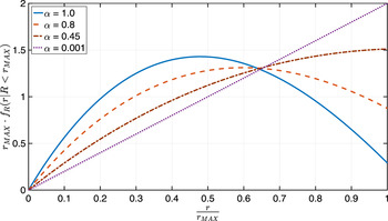
Figure A3 shows Equations (A11), (A12) and (A13) varying α = 1, 0.8, 0.45, 0.001, and must be compared with Figure 5.
Normalised conditioned density function with L = α·r MAX .