

For over 150 years, archaeologists have been reviewing and revising their methods on how best to document stratigraphic relationships during the process of archaeological excavation (for relevant discussions, see D'Amore Reference D'Amore and Smith2014; Demetrescu Reference Demetrescu2015; Harris Reference Harris2014; Higginbotham Reference Higginbotham1985; Huvila Reference Huvila2009). Some notable methodologies of stratigraphic documentation, still used in the present, include the Wheeler-Kenyon box grid (Kenyon Reference Kenyon1971; Wheeler Reference Wheeler1956) and the Harris Matrix (Harris Reference Harris2014). The Wheeler-Kenyon box grid is perhaps the most common and widely utilized method of stratigraphic documentation. It consists of the excavator placing balks at set intervals in between excavation units to form a grid from which stratigraphic relationships may be documented in vertical profile. However, such a system is only of limited use because archaeological deposits are often severely tilted, folded, or are restricted in their horizontal extent, making their identification across multiple spaced-out profiles extremely difficult and at times even impossible (Higginbotham Reference Higginbotham1985). Additionally, if balks are kept in place, it prevents the complete horizontal excavation of relevant deposits, such that much information is either lost or is never collected (Higginbotham Reference Higginbotham1985). The Wheeler-Kenyon method, therefore, forces a compromise between the preservation of the vertical and recovering the horizontal (Wheeler Reference Wheeler1956). An additional method, the Harris Matrix, although useful, is merely a representation of stratigraphic relationships in 2D diagram form that provides no visual facsimile of the field from which to make further assessments, interpretations, or corrections.
Along with the development of computing technologies, however, numerous new approaches have emerged by which archaeological data may now be collected and represented. One such approach is the systematic incorporation of photogrammetry in archaeological practice. Photogrammetry is often utilized to facilitate the 3D reconstruction of artifacts, sites, and archaeological deposits and features for their integration into a 3D GIS (Barceló and Vicente Reference Barceló, Vicente, Stadt Wien, Erbe and Wien2004; Beale and Reilly Reference Beale and Reilly2017; Chiabrando et al. Reference Chiabrando, D'Andria, Sammartano and Spanò2018; Chibunichev et al. Reference Chibunichev, Knyaz, Zhuravlev and Kurkov2018; Douglass et al. Reference Douglass, Lin and Chodoronek2015; Emmitt et al. Reference Emmitt, Pillay, Barrett, Middleton, Mackrell, Floyd and Ladefoged2021; Forte et al. Reference Forte, Dell'Unto, Issavi, Onsurez and Lercari2012; Gajski et al. Reference Gajski, Solter and Gašparovic2016; Hamilton and Stephenson Reference Hamilton and Stephenson2016; Katsianis et al. Reference Katsianis, Tsipidis, Kotsakis and Koussoulakou2008; Moya-Maleno et al. Reference Moya-Maleno, Valdelomar, Madrid and Sánchez2015; Nikolakopoulos et al. Reference Nikolakopoulos, Soura, Koukouvelas and Argyropoulos2017; Nobles and Roosevelt Reference Nobles and Roosevelt2021; Peng et al. Reference Peng, Lin, Guo, Wang and Gao2017; Walcek Averett et al. Reference Walcek Averett, Gordon and Counts2016), although best practices are under continued consideration (Dell'Unto et al. Reference Dell'Unto, Landeschi, Apel and Poggi2017; Fabio Reference Fabio2004; Galeazzi Reference Galeazzi2016, Reference Galeazzi2018; Galeazzi and Di Giuseppantonio Di Franco Reference Galeazzi and Di Franco2017; Gavryushkina Reference Gavryushkina2021).
In this article, we argue that new technologies such as photogrammetry, 3D modeling, and GIS do indeed offer us new possibilities for the documentation of complex stratigraphic relationships when systematically applied. By combining photogrammetric representations of horizontal surfaces excavated in stratigraphic succession, we can produce 3D models of archaeological deposits from which virtual cross sections may be generated. Our methodology, therefore, preserves and accurately reconstructs both the horizontal and the vertical dimension in such a way that serves to complement the existing methodologies of archaeological stratigraphic documentation. Here, we present the preliminary results of a pilot study, which began in 2013 and has continued until the present, developed during the excavations of the Chalcolithic layers at Tell Yunatsite, Bulgaria. Our preliminary results demonstrate that the systematic use of photogrammetry during the process of archaeological excavation provides a new and reliable means by which to document complex stratigraphic relationships.
CASE-STUDY: THE CHALCOLITHIC LAYERS AT TELL YUNATSITE, BULGARIA
Tell Yunatsite is located in the Upper Thracian Plain of Bulgaria and has been the subject of archaeological excavation since 1939 (Mikov Reference Mikov1940). It is a settlement mound composed of a medieval cemetery, a Roman fortification, two building levels from the Early Iron Age, 17 building levels from the Early Bronze Age, an approximate 1,000-year hiatus period, and a minimum of 11 building levels from the Early to Late Chalcolithic periods (Boyadzhiev et al. Reference Boyadzhiev, Boyadzhiev, Brandtstätter and Krauß2021). As of the most recent excavation season, there is also potential evidence of a Late Neolithic settlement at the site. The tell measures 110 m in diameter and stands 11 m above the modern-day terrain. Consequently, the site is a textbook example of complex archaeological stratigraphy, with each so-called building level or stratum containing thousands of individual depositional units aggregated in horizontal and/or vertical stratigraphic succession.
The Chalcolithic layers at the site make for a particularly relevant case study of our photogrammetry-assisted methodology for stratigraphic documentation. First, the excavation of the Chalcolithic layers at the site are ongoing, and since 2012, the context-based excavation system (see Renfrew and Bahn Reference Renfrew and Bahn2016) has been in use, such that every observable archaeological deposit is excavated and documented individually as opposed to immediately aggregated into features (i.e., as buildings, terraces, or building levels) or excavated by arbitrary levels (e.g., arbitrary “horizons” of 10 or 20 cm spits). Consequently, the excavation methodology in place already conforms to the laws and best practices of stratigraphic archaeological excavation as outlined by Harris (Reference Harris1975, Reference Harris1977, Reference Harris1979, Reference Harris1984, Reference Harris2014). Our photogrammetry-assisted methodology, therefore, rather than having been developed to replace existing best stratigraphic excavation practices, is designed to complement them. Our work then provides a reliable basis from which to suggest that the proposed methodology could be applied to other such archaeological excavations using similar excavation practices with little to no required adjustments.
Second, given that the site of Yunatsite represents a continuous occupation throughout the entire Chalcolithic period (as defined in Bulgaria; see Boyadzhiev Reference Boyadzhiev, Bailey, Panayotov and Alexandrov1995), understanding the stratigraphy of the Chalcolithic sequence at the site is of critical importance with regard to resolving several issues pertaining to the pan-regional rise and fall of the Late Chalcolithic Kodzhadermen-Gumelniţa-Karanovo VI cultural complex. Currently, there exists a debate as to the unscrutinized applicability of radiocarbon calibration curves for the region (see Tsirtsoni [Reference Tsirtsoni, Gori and Ivanova2017] for a relevant summary), which serves to highlight that absolute dates obtained from Late Chalcolithic sites often seem to overlap with those from the Middle Chalcolithic. The situation is no different even within a single site, as is demonstrated by the recent radiocarbon modeling of Tell Yunatsite (see Boyadzhiev et al. Reference Boyadzhiev, Boyadzhiev, Brandtstätter and Krauß2021). One side of the debate holds that the absolute dates are wrong and that a region-specific fluctuation in atmospheric 14C during the Late Chalcolithic period must exist, which results in absolute dates that are much too early for the period in question (Boyadzhiev Reference Boyadzhiev, Bailey, Panayotov and Alexandrov1995; Boyadzhiev and Aslanis Reference Boyadzhiev, Aslanis and Tsirtsoni2016; Boyadzhiev et al. Reference Boyadzhiev, Boyadzhiev, Brandtstätter and Krauß2021); the other side holds that the internal phasing of the Chalcolithic sequence, predominantly based on pottery typology, is wrong and is in need of considerable revision so as to better conform to the reported absolute dates (Boric Reference Boric, Kienlin and Roberts2009; Reingruber and Thissen Reference Reingruber and Thissen2009; Tsirtsoni Reference Tsirtsoni, Gori and Ivanova2017). Any resolution to such a debate will likely include aspects from both approaches, and although we do not immediately intend to resolve this debate here, we do suggest that a detailed intrasite context-based stratigraphic analysis of the Chalcolithic layers at Tell Yunatsite—as is facilitated by our proposed methodology of stratigraphic documentation—represents a critical step in the right direction.
DATA AND METHODS
Modeling the Site (i.e., the Settlement Mound)
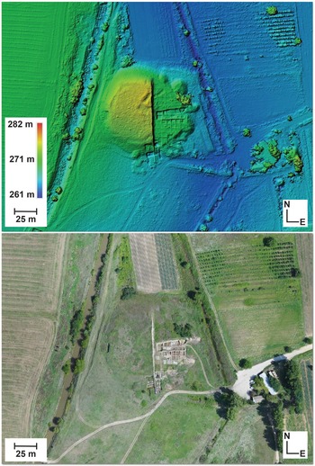
To model the site, we use the unmanned aerial vehicle (UAV) eBee senseFly drone and its associated eMotion 3 software package to set the flight path and select the desired image overlap and resolution parameters (for relevant technical details, see Chiabrando et al. Reference Chiabrando, D'Andria, Sammartano and Spanò2018:3), although any available drone with an onboard camera could conceivably arrive at the same or at least a similar result. We then choose to use Agisoft Photoscan Pro, version 1.4 (now rebranded as Agisoft Metashape) to align the captured images using the integrated GPS data appended to each photo, first to produce a sparse point cloud followed by a dense point cloud, and second, a 2.5D mesh of the entire settlement mound. We further identify the absolute xyz coordinates of ground control points (GCPs) using a total station to rectify and check the model geometry. The result is a georeferenced 2.5D terrain representation (DEM) of the entire settlement mound and its immediate surroundings (Figure 1).
Digital elevation model and orthophoto of Tell Yunatsite: (top) digital elevation model (DEM) and (bottom) orthophoto.

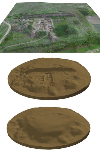
To transform the 2.5D photogrammetric representation of the site into a 3D volume, we utilize ArcGIS (ArcMap/ArcScene v. 10.5.1). First, we convert the DEM of the site into a triangular irregular network (TIN) and generate a constant bottom TIN (in this case, arbitrarily set 2 m below lowest surface level). We then use the Extrude Between tool available in the 3D analyst toolset of ArcGIS to fill the space between the top and bottom TINs to produce a geometrically accurate 3D volume of the entire site. Furthermore, given that the mound has been intermittently excavated since 1939, we reconstruct the excavated portions of the mound by using a topographic map of the site (compiled during the first excavation season; see Mikov Reference Mikov1940), from which we digitize the contour lines to produce an additional top TIN to then extrude between and fill the excavated portions of the mound. Both volumetric models are then joined to produce a final georeferenced 3D model of the settlement mound, as it was, prior to first excavation (Figure 2). The site model then serves as a “container” within which our additional excavation unit and depositional unit models can be placed to represent stratigraphic relationships relative to the entire site.
3D models of Tell Yunatsite: (top) 2.5D model, (middle) 3D model in its current state, and (bottom) 3D model prior to first excavation.

Modeling the Excavation Units (i.e., Grid Squares)
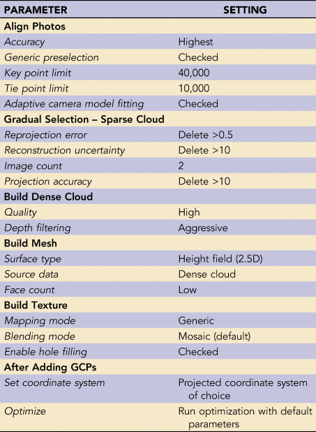
As previously noted, since 2012, the context-based excavation system has been in place at Tell Yunatsite in such a way that every single observable archaeological deposit is documented and excavated in stratigraphic order. We therefore excavate in stratigraphic succession within excavation units (i.e., 5 × 5 m grid squares) until a novel stratigraphic state is fully exposed in horizontal (i.e., until the boundaries of new contexts are exposed). When we reach a novel stratigraphic state within an excavation unit, we set a 1 × 1 m internal grid to be used as guides for photo acquisition and as GCPs for model georeferencing and rectification. We then proceed to systematically capture overhead photos using a Canon Powershot G12 camera with constant aperture (although any camera of choice would work—keeping the parameters and settings constant) of each square meter and between each square meter to ensure adequate image overlap (e.g., >60%; approximately 85 photos per 5 × 5 m unit) and pixel resolution (<1 cm2). The photos are then aligned using Agisoft Photoscan Pro v.1.4 (2018) to produce a sparse point cloud. The sparse point cloud is subsequently edited using the Gradual Selection tool available in Agisoft Photoscan Pro. All parameters for the Agisoft Photoscan model-building workflow are listed in Table 1.
Parameter Settings for the Production of 2.5D Excavation Unit Models Using Agisoft Photoscan Pro Version 1.4.

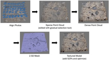
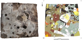
After having completed the Gradual Selection procedure, we proceed with the integrated model-building workflow to produce a dense point cloud, followed by a 2.5D mesh of the excavation unit, and finally, a textured 2.5D model of the excavation unit (Figure 3). Texturing is a process that consists of stitching the photos together to then drape over the 2.5D mesh, providing a photorealistic finish. After texturing, the internal 1 × 1 m grid markers, whose xyz coordinates are documented, serve as GCPs from which to georeference and rectify the model geometry. The model is then optimized to rectify any measurement errors using the Optimize Cameras tool and rerun in accordance with the GCPs so that a faithfully georeferenced and accurate 2.5D representation of the excavation unit is produced. A report of the model is then generated using Agisoft Photoscan Pro to ensure that the total geometric error does not exceed 2 cm. In our view, given that plan drawings of excavation units are typically produced at a 1 to 20 scale so that 1 mm on the page represents 2 cm on the ground, a global 2 cm margin of error for our models is acceptable and not overly problematic in terms of their eventual interpretation. Notably, if desired, a smaller margin of error can be achieved by taking more photos at smaller intervals and closer to the ground surface (e.g., every 0.5 m and between every 0.5 m) so that the resolution of the photos used in the modeling procedure is likewise increased. Finally, a 1:20 scale plan drawing of the excavation unit is produced by hand to document its current stratigraphic state (as is common archaeological practice) so that the outlines of individual archaeological deposits, the locations of artifacts, and other relevant information are documented (Figure 4). The plan drawings further serve as the basis from which the 3D models of archaeological deposits can subsequently be produced.
2.5D excavation unit model workflow, using Agisoft Photoscan Pro v. 1.4; GCPs = ground control points.

2.5D excavation unit model and (right) its corresponding plan drawing.

Modeling the Archaeological Deposits (i.e., Contexts)
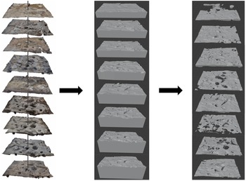
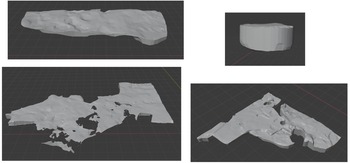
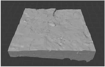
The next step in our photogrammetry assisted workflow consists of modeling each individual archaeological deposit in 3D. First, using the open source Blender version 2.8 software (https://www.blender.org/download/), we import and convert each 2.5D model of an excavation unit into a 3D solid by selecting the edges of the 2.5D model, extruding them to an arbitrary constant depth, and closing the resulting void to form a solid, making certain that every 3D model of an excavation unit partially overlaps with its corresponding model below. We then use the Boolean Difference modifier included in Blender to subtract the models below from the models above so that we are left with a series of 3D solids that represent only the excavated volumes between successive stratigraphic surfaces (Figure 5). Next, we digitize the horizontal boundaries of our archaeological deposits in GIS as they appear in each successive surface model and their associated plan drawings. Using the BlenderGIS Addon (https://github.com/domlysz/BlenderGIS), we then import the context boundaries to Blender as georeferenced shapefiles, select their edges, extrude to an arbitrary height and depth to surpass the thickness of its related excavated volume models, and use the Boolean Intersect modifier available in Blender to extract the portion of the excavated volume models that intersect with the appropriate context boundary model—an approach that we have taken to calling the “cookie-cutter method.” After having repeated the process for each individual archaeological deposit present within the excavation unit across all excavated surfaces, we use the Boolean Union modifier to merge all portions of the same archaeological deposit into a single model and use the Voxel Remesh modifier available in Blender (at 0.5 × 0.5 cm resolution) to produce a topologically coherent 3D manifold mesh of the archaeological deposit in question (Figure 6). The end result is a geometrically faithful series of 3D models representing every unique archaeological deposit in the excavation unit. The 3D models can then be imported into a 3D GIS to produce block models of the excavation units for the purposes of virtual cross sectioning (Figure 7) or to serve as “objects” in an object-relational GIS to conduct geospatial analyses, calculate volumes, or perform any number of querying operations that may be relevant to the continued interpretation of the site.
From 2.5D to 3D: (left) series of 2.5D excavation unit models in stratigraphic succession, (middle) series of 3D solid excavation unit models in stratigraphic succession, and (right) series of 3D excavated volume models in stratigraphic succession. Note that vertical exaggeration is applied between each unit model for visualization purposes; total depth is approximately 60 cm excluding dug-in structures.

Examples of 3D archaeological deposit models.

3D block model of archaeological deposits in a single excavation unit.

Producing Virtual Cross Sections
The final step in our workflow for the documentation of complex stratigraphic relationships using photogrammetry is the production of virtual cross sections. The process can be undertaken in several different ways. One approach is to use the profile graph tool available in ArcGIS over the resulting 3D block models of the excavation units, although the produced graph is sensitive to scale, and the output format is neither entirely conducive to modification or labeling nor is otherwise useful for the production of easily interpretable visualizations. An additional possibility is to use the Boolean modifiers available in ArcGIS to extract the portions of the block models that intersect with any user-defined rectangle parallelepiped, although if any of the context models are not perfectly manifold, the system will crash and return an error. Unfortunately, several of the context models, despite conforming to manifold principles when produced in Blender, become nonmanifold (for some as-yet-unknown technical reason) once imported into ArcGIS. For this reason, we suggest that the production of cross sections be performed directly in Blender, because it is by far the simplest and most consistent approach and because it produces the best and most readily interpretable results.
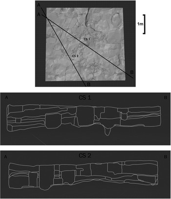
To produce cross sections in Blender, one simply joins all relevant archaeological deposit models into a single object from which the bisect tool can be used. Then, using the bisect tool available in Blender, a cross-section line can be drawn over the model and the resulting selection can be separated into a distinct object representing a vertical cross section (Figure 8). The output can then be exported as an image (screenshot; Blender render) or as a shapefile (using the BlenderGIS Addon) for the purposes of labeling or to make other modifications in any software of choice (e.g., ArcGIS, CorelDRAW, Adobe Illustrator, etc.). Most notably, our method allows for cross sections to be produced from anywhere in the excavation unit and between several different excavation units, enabling stratigraphic assessments between any and all documented archaeological deposits. In other words, profile drawings of the stratigraphic relations between contexts can be produced without the need to maintain a physical balk or vertical profile during the process of archaeological excavation. Field notes regarding stratigraphic relationships can also then be checked against the digital record to ensure that all stratigraphic relations between contexts have, indeed, been accounted for prior to building a Harris Matrix.
Examples of virtual cross sections produced from 3D block model of archaeological deposits.

Data Management Plan
By using the proposed methodology, a number of digital datasets are produced for which a viable data management plan is necessary. Considering that the excavation units are labeled in accordance with an alphanumeric (5 × 5 m) grid, we adopted a naming convention based on the alphanumeric identifiers of each excavation unit, followed by the number of the excavation unit model in its stratigraphic sequence (from top to bottom). For ease of access and maneuverability, each separate dataset is stored in a parent folder. Concerning the photographs taken for the structure-from-motion photogrammetry procedure, they are first stored in a parent folder named “Agisoft_Photos” as JPGs and organized in subfolders matching the alphanumeric identifier of the excavation unit to which they refer and the number of the model in its stratigraphic sequence (e.g., O7_1, O7_2, O7_3, O7_4, etc.). The coordinates of GCPs are stored as text files under the parent folder “Agisoft_markers” and, again, named by the alphanumeric identifier of the excavation unit and the number of the model in its stratigraphic sequence (e.g., O7_1, O7_2, O7_3, O7_4, etc.). The Agisoft Photoscan projects and related files are stored in a parent folder named “Agisoft_Pro,” and each project, again, is named by the alphanumeric identifier of the excavation unit and the number of the model in its stratigraphic sequence (e.g., O7_1, O7_2, O7_3, O7_4, etc.).
From each Agisoft project, a number of additional outputs are produced. These are the 2.5D excavation unit models, stored as Collada files under the parent folder “Agisoft_Collada,” excavation unit orthophotos stored as TIFFs under the parent folder “Agisoft_Orthophotos,” and the accuracy reports stored as PDFs under the parent folder “Agisoft_Reports,” each conforming to the alphanumeric and model-number naming convention. Notably, the accuracy reports also include the precise date on which the modeling procedure took place in the field so that the models can be correlated with relevant field notes and other forms of documentation. Plan drawings produced in the field are scanned, georeferenced, and stored as TIFFs named with the alphanumeric identifier of the excavation unit followed by the date, which matches the date of the 2.5D model noted on the accuracy reports (e.g., O7_DDMMYY). The whole is then aggregated into an Excel spreadsheet, with the column labels Model_ID, Date, Agisoft_Project, Markers, Ortho, Plan, and Report. The Model_ID column is populated with the alphanumeric and model number identifier, the Date column is populated with the date on which the model was produced in the field, and the remainder are populated by hyperlinks to their relevant datasets.
The digitized context boundaries produced from the plan drawings are stored as shapefiles in a parent folder named Plan_Shapefiles and labeled with the alphanumeric and model number identifier (e.g., O7_1, O7_2, O7_3, etc.). The Blender projects are saved in a parent folder named Blender_Projects, labeled only by the alphanumeric identifier of the relevant excavation unit (e.g., O7, M4, H6), which houses all of the 3D context models pertaining to that unit. The individual 3D context models are then exported as Collada files and labeled by their unique context ID (e.g., Cont_100, Cont_47, Cont_99). Note that each context identified on the site is given its own unique ID number. Should a unit specific system be in place, the naming convention can be modified to first note the grid unit's ID (e.g., Cont_M4_2, Cont_H6_2, Cont_O7_2, etc.). All context models are then imported into a master 3D GIS of the entire archaeological excavation, and virtual cross sections are produced in Blender according to interpretive need. In all cases, the specific file types were selected first and foremost because of their lossless data qualities and because of their ease of interoperability relative to the utilized software (i.e., ArcGIS, Blender, and Agisoft Photoscan).
RESULTS
To date, using the present methodology, we have mapped approximately 3.75 km2 of the modern-day terrain at 10 cm resolution, representing the entire site and a significant portion of its immediate surroundings. Such outputs can be used to conduct further landscape analyses and to elaborate on site geomorphology and formation processes. Additionally, we have produced over 80 individual 5 × 5 m excavation unit models at <1 cm resolution, which are useful as graphic documentation of the excavation process in conjunction with their associated technical plan drawings. Finally, from the excavation unit models, we have documented the top and bottom boundaries of nearly 700 individual archaeological deposits—spanning the Early to Late Chalcolithic periods—that can subsequently be reconstructed and represented in true 3D using the photogrammetry-assisted methodology from which virtual cross sections can also be produced to aid in the interpretation of complex stratigraphic relationships.
DISCUSSION
Following from our experience using the proposed methodology over the course of eight excavation seasons—from 2013 to the present—we can confidently state that it is not only effective but that it requires next to no modifications to the existing context-based archaeological excavation practice. Consequently, the implementation of our method proves to be time effective and does not set back the progress of excavation in any meaningful way. In short, the excavators continue to excavate as usual, and when a new stratigraphic state is uncovered within the excavation unit, a 1 × 1 m grid is added, and the overhead photos are captured for structure from motion photogrammetry undertaken at the same time as the process of plan drawing. Given an appropriate run-of-the-mill computer that meets the minimum requirements of GIS, the photogrammetric models of the excavation units can then be produced overnight and verified on the spot before excavation in the unit continues. Only in a few rare instances, related to blurry photos or inadequate overlap between photos (predominantly encountered during the first trial years), was excavation ever completely halted within a single excavation unit until such problems with photo acquisition could be resolved. Even so, it rarely took more than an additional day to rectify any errors. Once we had completely worked out the specifics of our systematic approach, we experienced no delays to the excavation process at all. The only true additional requirement is an individual who is at least partially dedicated to the production and verification of the photogrammetric models on site and in a timely fashion.
Furthermore, with the exception of the eBee senseFly drone and its associated eMotion 3 software—which conceivably could be replaced by any commonly available commercial drone with an onboard camera—the needed technologies are also not overly cost prohibitive. As photogrammetry becomes more and more common in a number of different disciplines, so too are institutional licenses for the required software(s). Additionally, Blender is open sourced and freely available—as are a number of GIS platforms with 3D capabilities. The only other piece of technology required is a run-of-the-mill camera, which we posit is already part of any archaeologist's regular tool kit. Although a total station can certainly be of use—and, indeed, is best practice—the process of coordinate retrieval for ground control points can equally be undertaken by carefully using a plumb bob, measuring tape, and dumpy level. Therefore, in comparison with other such methods that utilize laser scanners or top-of-the-line robotic total stations to obtain the same or at least similar results, our methodology is extremely cost effective. Depending on the scale of the excavation, it is recommended that dedicated hard drives be purchased for the storing and handling of the digital data.
Having addressed the viability of our proposed methodology for almost any conceivable archaeological excavation utilizing a context-based excavation method, we now turn to some of the embedded assumptions and limitations. First, our method, as stated, assumes that a context-based excavation practice is utilized on site so that every relevant archaeological deposit is excavated and documented in stratigraphic succession rather than by composite feature or arbitrary depth. Following from the assumption that a context-based excavation practice is utilized, it also then assumes that every individual archaeological deposit is visible and, consequently, is recognizable in the field. It then follows that if an archaeological deposit is not visibly distinguishable from its immediate neighbors, it and the others will likely be interpreted in aggregate form as a single deposit, when in fact they are many chronologically distinct deposits. Distinguishability is, however, only a problem in stratigraphic terms if the aggregated deposit in question possesses any paradoxical associations with other unique deposits, which becomes an issue of excavation practice rather than an issue with our proposed methodology. One might consider, for example, the case where several chronologically unique artifact scatters (i.e., unique archaeological deposits) are contained within a single long-lived layer having the same or at least a visibly similar sediment matrix (i.e., a unique geological deposit). In such cases, although the artifact scatters may not be distinguished as stratigraphically unique and precision is lost, the layer itself should have no paradoxical stratigraphic relationships with other such visibly distinct layers. A decision must then be made from the outset as to whether artifact scatters should be designated as separate archaeological deposits, and modeled as such, even if they are contained within the same long-lived geological deposit (e.g., within the same layer of sediment) for the proposed methodology to remain viable. Ultimately, whether or not our methodology is effective will depend on the nature of the deposition process on site and the chosen excavation method. We hold, however, that such homogenous geologic strata containing numerous distinct archaeological deposits are not typically encountered during the excavation of settlement mounds, which are predominantly structured by human rather than by natural action. Should excavators wish to employ the methodology here presented to address even more complex stratigraphies, such as are most often encountered on the excavation of Paleolithic sites, the geometric margin of error for the models can be made finer by increasing the pixel resolution of the photos taken. Furthermore, confounding deposits (such as animal burrows, large boulders, or undercuts) can be accounted for and included in the modeling process by following the same principles as all other deposits.
Second, given that the production of the 3D archaeological deposit models depends entirely on the systematic production of the 2.5D excavation unit models, it follows that a problem with the latter process will cause irreversible problems with the former. In short, every archaeological deposit, depending on its geometric complexity, must be represented in at least two of the excavation unit models without fail—one surface that represents its topmost boundary, and a second representing its bottommost boundary. In the case that two distinct archaeological deposits are excavated in vertical succession without a corresponding 2.5D model having been produced in the interim, the exact stratigraphic boundary between those deposits will be lost, and one must resort to other means of reconstruction. It cannot, therefore, be stressed enough that our methodology wholly depends on the accuracy and systematic application of a stratigraphic excavation process. It should also be noted that, in some instances, our methodology actually allowed us to retrieve stratigraphic information that beforehand was not recognized in the field. For example, the topmost boundaries of certain structures (such as pits and ditches) were subsequently visually recognized in excavation unit models that had been made prior to their formal topmost identification in the field. Our methodology, therefore, unexpectedly allowed us to correct and revise some aspects of our stratigraphic documentation that had beforehand gone unrecognized. To summarize, the viability of the photogrammetry-assisted methodology presented here depends on establishing a systematic approach toward excavation unit modeling that works well for the site in question and the excavation procedure in place.
Regarding the interpretative potential of the proposed methodology, it follows that the ability to produce virtual cross sections from anywhere on the site provides a means to view and verify the stratigraphic relationships of any and all archaeological deposits so that artifact seriations and Bayesian chronologies can likewise be made more informative and precise. Furthermore, because the production of stratigraphic profiles is not limited by the maintenance of physical balks during the process of archaeological excavation, the orientation, thickness, and dip of archaeological deposits can be more easily assessed and understood dynamically because they can be cross-sectioned and viewed from any angle. Last but not least, by combining the 3D models of all archaeological deposits into a 3D GIS, we can obtain a true 3D depiction of the archaeological site from which any number of spatial analyses and attribute queries can be performed.
CONCLUSION
The proposed photogrammetry-assisted methodology for the documentation of complex stratigraphic relationships indeed serves as a complement to the existing methodologies of archaeological stratigraphic documentation—namely, the Wheeler-Kenyon box grid method and the Harris Matrix. Most of all, it compensates for the shortcomings of these existing methodologies. Unlike the Wheeler-Kenyon method, the production of cross sections using our method is not limited only to spaced-out intervals. Instead, cross sections can be produced from anywhere within or between excavation units, making the interpretation of stratigraphic relationships all that much more intuitive and situation specific. It also allows for the production of Harris Matrices by the postexcavation dynamic visualization of 3D archaeological deposits and their relative positions rather than from static written notes based on the excavator's observations made in the field, which makes postexcavation corrections and assessments possible. Ultimately, it is our hope that the method presented here will also allow for the creation of a true 3D GIS of the entire archaeological site, complete with searchable attribute tables and catalog relates that would facilitate innumerable types of postexcavation analyses and serve as a retrievable resource for future researchers and for educational purposes. The creation of a true 3D GIS of archaeological excavations is an end goal that has long been conceptualized but to date has remained almost completely unattainable or, at best, only partially achieved. However, given the success of our method as here presented, we believe that the achievement of such an end goal lies in the very near future. We remain committed to examining directions for future research.
Acknowledgments
The archaeological excavations, from which the work herein is derived, were undertaken with permission from the Ministry of Culture of the Republic of Bulgaria and financially supported by the Ministry of Culture of the Republic of Bulgaria, the Pazardzhik Regional Museum of History, and the Balkan Heritage Foundation. An earlier draft of this manuscript was presented at the 26th Annual European Association of Archaeologists Conference (Virtual), Session 21: “Archaeology in 3D: New Technologies for Old Questions.” We wish to thank the session organizers and participants for their very useful suggestions and comments, which positively contributed to the final draft.
Data Availability Statement
Data are curated at the National Archaeological Institute with Museum, Bulgarian Academy of Sciences. Contact: Kamen Boyadzhiev, 2 Saborna St., 1000 Sofia, Bulgaria (e-mail: kamenyb@abv.bg).
Competing Interests
The authors declare none.