1 Introduction
The advent of the turbojet engine led to a transformation in both commercial and military aviation, enabling much faster flight than previously possible with propeller-driven aircraft. However, the increased thrust of turbojets (followed by turbofans) is not without negative consequences: significant acoustic radiation is generated by the exhaust jet. This has spurred extensive research into the acoustic source mechanism in high-speed, high Reynolds number jets. While progress has been made in the field of aeroacoustics, understanding of jet noise sources and their radiation mechanisms remains incomplete (Jordan & Gervais Reference Jordan and Gervais2008). This is due to the large number of interrelated parameters (e.g. Reynolds number, temperature ratio, acoustic Mach number, nozzle geometry, etc.) as well as the large disparity in the length and time scales associated with the turbulent phenomena and the radiated noise. As a result, current noise-mitigation technologies for free jets have largely been applied in an ad hoc manner. Fully realizing this maximum noise reduction potential will require a much more detailed understanding of the mechanisms by which free jets produce noise which radiates to the far field.
It is generally agreed that the dominant noise sources in high-speed jets are related to the large-scale coherent structures which have been identified in the mixing layer of the jet (Arndt, Long & Glauser Reference Arndt, Long and Glauser1997). As discussed by Tam (Reference Tam1995) (among others), large-scale structures can be represented as instability waves superimposed upon the mean flow. At subsonic convection velocities, a plane instability wave with fixed frequency/wavenumber will emit no acoustic radiation to the far field. However, modulation of the instability wave’s amplitude creates a dispersion in the energy content of the instability wave. By doing so, the broadband instability wave, commonly referred to as a wavepacket, can shift energy to supersonic phase velocities and hence produce sound which radiates to the far field. Wavepacket models for noise emission have become commonplace, owing to their great success at predicting low-angle acoustic emission relative to the jet axis (Obrist Reference Obrist2011). Simple linear wavepacket models have allowed researchers to probe different aspects of the waveform modulation, in turn illuminating possible relevant dynamic behaviour of the large-scale structures for the noise generation process. Temporal modulation of the wavepacket’s amplitude and spatial extent (‘jittering’) were shown to increase the efficiency of the noise source (Cavalieri et al. Reference Cavalieri, Jordan, Agarwal and Gervais2011); this conforms to experimental results which have indicated that the noise generation in free jets is highly intermittent (Juvé, Sunyach & Comte-Bellot Reference Juvé, Sunyach and Comte-Bellot1980; Hileman et al. Reference Hileman, Thurow, Caraballo and Samimy2005; Kearney-Fischer, Sinha & Samimy Reference Kearney-Fischer, Sinha and Samimy2013). Although progress has been made in experimentally measuring wavepacket characteristics in high-speed turbulent jets (Cavalieri et al. Reference Cavalieri, Rodriguezl, Jordan, Colonius and Gervais2013; Baqui, Agarwal & Cavalieri Reference Baqui, Agarwal and Cavalieri2014), a direct link between large-scale structure dynamics and the aeroacoustic source has remained elusive.
In tandem to instability analysis of the noise source mechanism, the development and refinement of acoustic analogies has occurred. Lighthill (Reference Lighthill1952) was the first to reorganize the Navier–Stokes equations into a linear wave equation with a quadrupole-like source term comprising density, Reynolds stress and entropic fluctuations. Work by Phillips (Reference Phillips1960), Lilley (Reference Lilley1974), and much later Goldstein (Reference Goldstein2003) extended this formulation to include convective effects of the ambient medium, thereby separating the true sound sources in Lighthill’s acoustic analogy from purely propagative effects. Alternative approaches were also developed by Ribner (Reference Ribner1962), Powell (Reference Powell1964) and Howe (Reference Howe1975) (the last of which will be used in the current work). These sought to better connect the acoustic source mechanisms to distinct physical phenomena occurring in the turbulent shear layer. In a similar vein, Cabana, Fortuné & Jordan (Reference Cabana, Fortuné and Jordan2008) decomposed Lighthill’s acoustic source term into sub-terms of velocity, vorticity, dilatation and density fields in order to understand the relative (and sometimes competing) roles each had in the noise generation process. Ultimately however, a clear distinction between efficiently and non-efficiently radiating structures has not been defined.
The purpose of this work is to examine the dynamic evolution of the large-scale coherent structures which lead to the dominant mixing noise in a subsonic, turbulent jet. The focus will be on the axisymmetric, toroidal vortices (azimuthal Fourier mode zero), as these are known to dominate both the near-field pressure and the acoustic far-field (Juvé, Sunyach & Comte-Bellot Reference Juvé, Sunyach and Comte-Bellot1979; Arndt et al. Reference Arndt, Long and Glauser1997; Hileman et al. Reference Hileman, Thurow, Caraballo and Samimy2005; Kœnig et al. Reference Kœnig, Cavalieri, Jordan, Delville, Gervais and Papamoschou2013); Jet instabilities will therefore be excited using localized arc-filament plasma actuators (LAFPAs) in order to generate these axisymmetric structures with a well-defined temporal frequency and phase. The irrotational near-field pressure will be acquired via a linear array of microphones, and decomposed into its constitutive acoustic and hydrodynamic components to identify the dominant noise source region. Time-resolved velocity fields will then be estimated based on stochastic correlations between the near-field pressure and the orthogonal modes of ensemble (non-time-resolved) velocity data, identified by an artificial neural network. From these time-resolved fields, the coherent structure dynamics will be identified and in doing so, the structure dynamics will be directly linked to the acoustic source region.
2 Experimental methodology
All experiments were conducted at the Gas Dynamics and Turbulence Laboratory’s (GDTL) anechoic chamber, details of which can be found in Hahn (Reference Hahn2011). The dimensions of the chamber are 6.20 m wide by 5.59 m long and 3.36 m tall, with internal wedge-tip to wedge-tip dimensions of 5.14 by 4.48 m and 2.53 m, respectively. The design of the chamber produces a cutoff frequency of 160 Hz, below the frequencies of interest for this study. Compressed, dried and filtered air is supplied to the facility from two cylindrical storage tanks with a total capacity of
 $43~\text{m}^{3}$
and maximum storage pressure of 16 MPa. The air may be routed through a storage heater, which allows the jet to operate with a stagnation temperature up to
 $500~^{\circ }\text{C}$
, before expanding through a nozzle and exhausting horizontally into an anechoic chamber. As the current work was focused on a cold jet, the heater was rarely necessary; in certain circumstances though (namely, long experimental runs) the heaters were used to slightly preheat the flow, thereby mitigating the temperature drop as the storage tanks were drained of high-pressure air. Opposite the nozzle, a collector accumulates the jet and exhausts to the outdoors.
For this work a converging, axisymmetric nozzle with exit diameter
 $D$
of 25.4 mm was used. The nozzle was a thick-lipped design in order to simplify the mounts for the plasma actuator extension, which housed the eight actuators used in this study. The jet was operated at a Mach number (
 $M_{j}$
) of 0.90, and with a total temperature ratio of approximately unity, resulting in a Reynolds number based on the jet exit diameter was
 $6.2\times 10^{5}$
. Previous investigations using hot-wire anemometry have indicated that the initial shear layer is turbulent for this operating condition with momentum thickness 0.09 mm and boundary layer thickness
 ${\sim}1~\text{mm}$
(Kearney-Fischer, Kim & Samimy Reference Kearney-Fischer, Kim and Samimy2009).
2.1 Localized arc-filament plasma actuators
The design of the LAFPAs, as well as the driving circuitry, has undergone a slow evolution since their initial development; a detailed description of initial development and LAFPA characteristics can be found in Utkin et al. (Reference Utkin, Keshav, Kim, Kastner, Adamovich and Samimy2007). In the current work, each LAFPA consists of a pair of 1 mm diameter tungsten pin electrodes, spaced 4 mm apart at their tips (centre-to-centre). The eight actuators were uniformly spaced around the nozzle perimeter 1 mm upstream of the nozzle exit. For electrical and thermal durability, the electrodes were housed in a boron nitride extension attached to the end of the nozzle. A groove with dimensions of 1 mm wide and 0.5 mm deep is machined in the boron nitride, into which the electrode tips protrude; this provides a region of low momentum flow in order to stabilize the plasma arcs. It has been shown that the existence of this groove does not substantially alter the flow field or the control authority of the LAFPAs (Hahn, Kearney-Fischer & Samimy Reference Hahn, Kearney-Fischer and Samimy2011).
The LAFPAs were energized by a multi-channel, high-voltage plasma power generator capable of simultaneously powering up to eight LAFPAs, which was designed and built in-house at the GDTL. In this second-generation power supply, each individual circuit consists of a switchable capacitor in line with a high voltage transformer; the arcing electrodes are connected to the secondary side of the coil. The capacitor is charged by a 100 V DC power supply when the first switch is closed and the second is opened; at the user-specified time the switches flip and it discharges through the coil. The switches are controlled by a 16-channel digital I/O card and National Instruments’ Labview software, operated by a dedicated computer. The plasma generator provides independent control of the frequency, duty cycle/pulse width, and phase (though not the amplitude) of each individual actuator. The pulse width was held constant at
 $7~\unicode[STIX]{x03BC}\text{s}$
, which was found to be the minimum pulse width at which the actuators consistently arced for all frequencies explored in this study (Hahn et al.
Reference Hahn, Kearney-Fischer and Samimy2011).
The spatially discrete nature of LAFPAs means that energetic fluctuations of higher order (relative to the fundamental excitation mode) are generated by excitation. Experimental quantification of this is difficult at the nozzle exit, due to the potential of damage to physical probes from the plasma and electrical discharge as well as saturation of optical measurement systems. However, it has been shown in Sinha (Reference Sinha2011) that upstream of the end of the potential core, the near-field pressure of a subsonic jet was dominated by the axisymmetric azimuthal Fourier mode when excited with
 $m=0$
near the jet column frequency. High-fidelity simulations of a supersonic jet by Gaitonde & Samimy (Reference Gaitonde and Samimy2011) demonstrated coherent (though complex) ring vortices being generated by heuristically modelled
 $m=0$
LAFPA excitation. Therefore, it is reasonable to assume azimuthal symmetry for the excited jet in the current work.
2.2 Time-resolved pressure
Near-field and far-field pressure measurements were acquired using Brüel & Kjær 0.25-inch 4939 microphones and preamplifiers. The signal from each microphone is band-pass filtered from 20 Hz to 100 kHz using a Brüel & Kjær Nexus 2690 conditioning amplifier, and recorded using National Instruments PXI-6133 A/D boards and LabVIEW software. The microphones are calibrated using a Brüel & Kjær 114 dB, 1 kHz sine wave generator (type 4231). The frequency response of the microphones is flat up to roughly 80 kHz, with the protective grid covers removed.
Far-field acoustic pressure is acquired at three polar angles:
 $30^{\circ }$
,
 $60^{\circ }$
and
 $90^{\circ }$
, as measured from the downstream jet axis. The microphones were oriented such that they are at normal incidence to the jet downstream axis at the nozzle exit. The radial distance of the microphones ranges from
 $101D$
at
 $30^{\circ }$
to
 $145D$
at
 $60^{\circ }$
, with
 $90^{\circ }$
at an intermediate position.
The near-field pressure was acquired during two separate experimental campaigns; the first focusing purely on the near-field and far-field pressure and the second focusing on the instantaneous velocity field. During the first campaign, the irrotational near-field was acquired using a linear array of sixteen microphones located along the meridional plane of the jet; the spacing varied along the array from
 $1D$
to
 $2D$
. The array was inclined at an angle of
 $8.6^{\circ }$
to the jet axis in order to match the spreading angle of the jet shear layer (Kearney-Fischer et al.
Reference Kearney-Fischer, Kim and Samimy2009), and the first microphone was positioned at
 $x/D=1,r/D=1.2$
. Voltage signals were collected at 200 kHz with 81 920 data points per block; ten blocks were recorded for each case resulting in four seconds of data, which had been found to be sufficient for statistical convergence.
In the second experimental campaign, a shorter array consisting of 12 microphones equally spaced by
 $1D$
was used. In this case, the array was mounted from the floor and at an angle off the meridional plane of the jet (with microphone tips angled normal to the jet axis). This set-up was used in conjunction with the particle image velocimetry described in the following section; the microphone array was placed off of the meridional plane so that it did not intersect with the laser sheet. As before, the microphone array was angled
 $8.6^{\circ }$
with respect to the jet axis, and the axial and radial positions were set to match the closest microphone array location used during the first experimental campaign. Voltage traces were acquired at 400 kHz, with 24 576 points collected per block. The voltage traces were collected simultaneously with streamwise particle image velocimetry measurements; 1500 blocks were acquired, corresponding to the 1500 acquired images.
In addition to the microphone voltage traces, the acoustics data acquisition system recorded a reference signal corresponding to the LAFPA excitation. The TTL pulse sequence, which controls the LAFPAs, was supplied to an Agilent 3320A waveform generator. The rising edge of the TTL pulse triggered a sharp drop in the output voltage of the waveform generator, which then ramps back up to the original voltage over a time interval which is shorter than the minimum excitation period. The output from the waveform generator was acquired simultaneously with the near- and far-field pressure signals using the aforementioned National Instruments hardware and software. As the excitation frequency, azimuthal mode, and ramp signal are well defined, this system enables the identification of the zero phase of actuation and hence, the ability to phase-average the pressure signals over the excitation period, akin to the work performed in Sinha et al. (Reference Sinha, Alkandry, Kearney-Fischer, Samimy and Colonius2012).
2.3 Snapshot particle image velocimetry
The instantaneous velocity was acquired using planar streamwise, two-component particle image velocimetry (PIV). A Spectra Physics, double-pulsed Nd:YAG laser (model PIV-400) was used as the illumination source with a time delay of
 $3~\unicode[STIX]{x03BC}\text{s}$
between the two laser pulses. It was observed that the actual time delay produced by the PIV system did not match the delay specified in the control software; instead, it would drift on a day-to-day basis by up to 10 %. This resulted in incorrect velocities being computed by the cross-correlations. In order to correct for this, the laser pulses were recorded using a ThorLabs DET210 photodetector and a LeCroy Wavejet 324A oscilloscope; the final vector fields were linearly scaled based on the ratio between the specified time delay and the measured time delay.
The jet core was seeded using Di-Ethyl-Hexyl-Sebacat (DEHS); the oil was atomized using a LaVision Aerosol generator and injected upstream of the turbulence screens in the stagnation chamber in order to produce a uniform seed particle density. As the jet entrains a significant amount of the surrounding ambient fluid as it evolves downstream, the coflow around the jet must also be seeded in order to accurately measure the outer shear layer velocity. For this, a TSI 6-jet atomizer was used to inject olive oil into a plenum. Per the manufacturer’s specifications, both atomizers provided nominally sub-micron seed particles. To ensure consistent seeding, this coflow was driven using a small blower and a series of small ejectors.
Image groups were acquired using two LaVision Imager Pro SX 5M cameras, which had 12-bit resolution and
 $2560\times 2180~\text{pixels}$
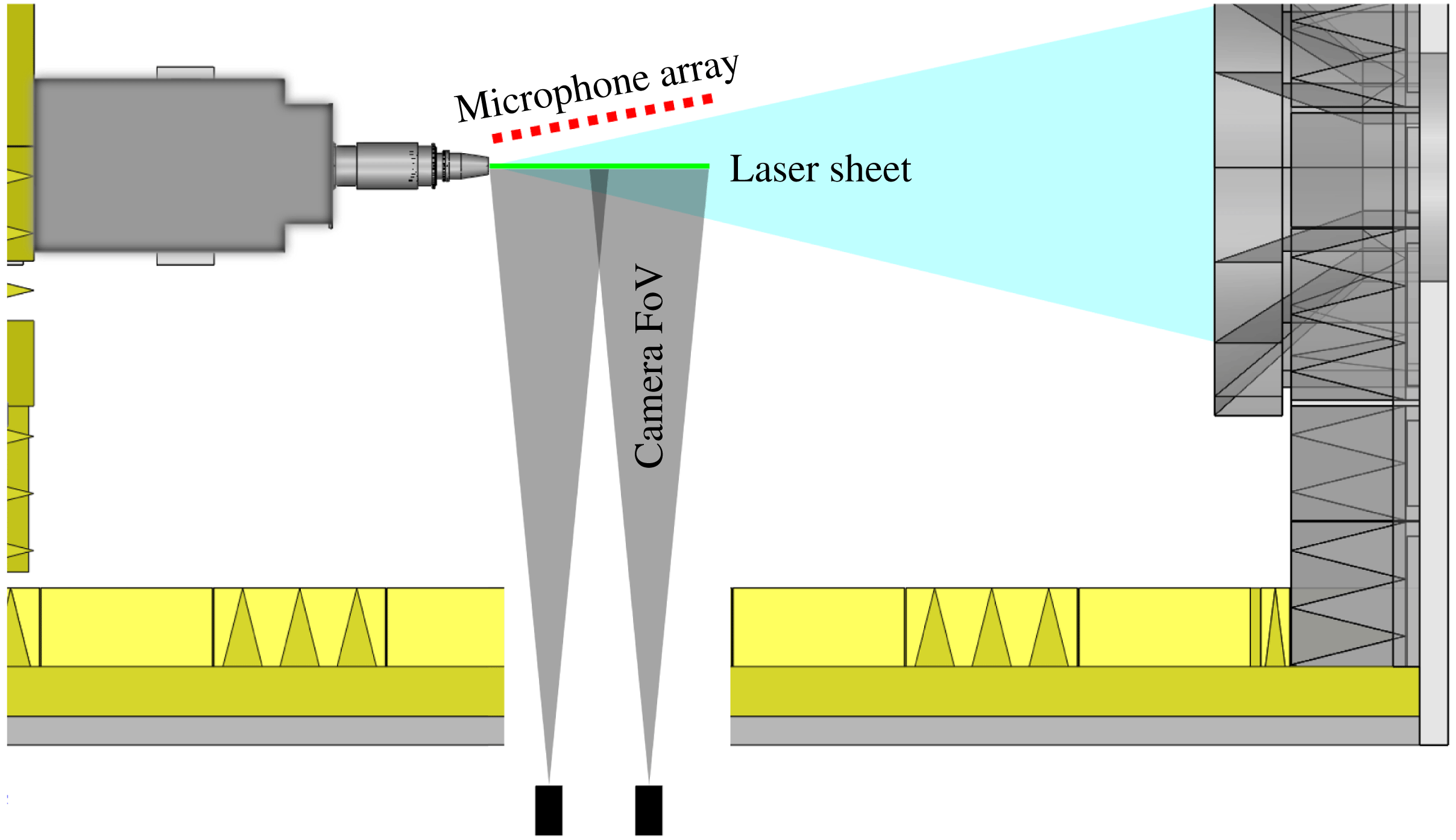
. The combination of the PIV-400 laser and the Imager Pro SX cameras resulted in a maximum acquisition rate for the image groups of 5 Hz. The cameras were positioned such that they were nominally normal to the image plane, negating the need for scheimpflug mounts. This was done as having high spatial resolution and field of view were deemed to be more important than having full, three-component velocity vectors. This set-up is generally designated as ‘side-to-side’ in order to differentiate it from stereoscopic PIV; a schematic of the set-up can be found in figure 1.
Schematic of syncronized PIV and near-field pressure data acquisition set-up.

The image groups were acquired randomly in time (i.e. uncorrelated to the pressure data acquisition) at the system’s maximum acquisition rate. The PIV computer was set to output a reference signal which was used to trigger the microphone data acquisition system. The timing was set such that the PIV image acquisition would occur roughly in the centre of a data block acquired by the acoustics system; the signal from a photoreceiver was also recorded in order to accurately identify the timing of the image acquisition in relation to the pressure time traces. For this case, 1500 image groups were acquired for each case.
Instantaneous velocity vectors were computed using LaVision’s DaVis software. Multipass, FFT-based cross-correlations were used, with decreasing window size (
 $64\times 64$
for the initial pass, and
 $32\times 32$
for the final three passes). A 50 % overlap was used for the initial pass, and a 75 % overlap was used for all subsequent passes; this produced a final grid of
 $563\times 258$
vectors at
 $0.58~\text{mm}\times 0.58~\text{mm}$
spacing. The velocity fields were post-processed to remove spurious vectors, which were iteratively replaced if secondary correlation peaks were found, before the downstream and upstream images were combined. No interpolation, smoothing, or denoising was performed in post-processing. The vector fields produced by the two cameras were then stitched together in DaVis using a common origin provided by a LaVision Type 31 calibration plate.
3 The near- and far-field response of the jet to excitation
3.1 Previous results
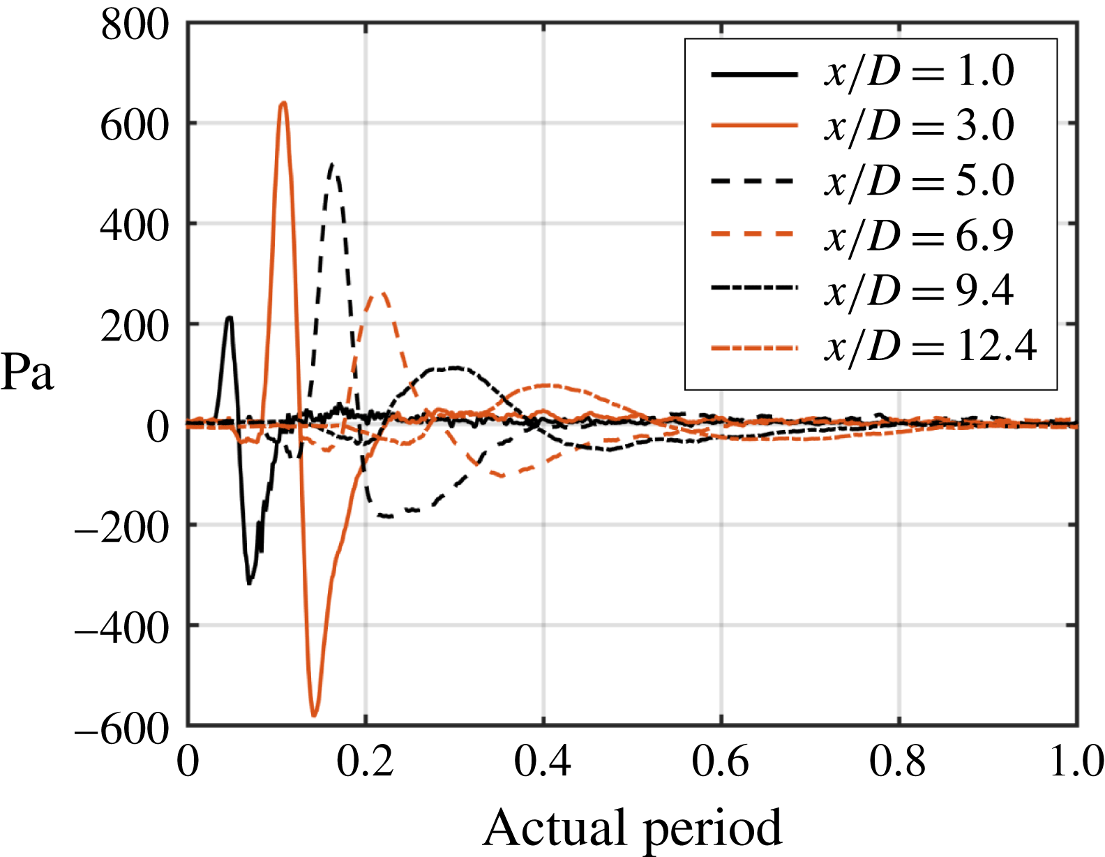
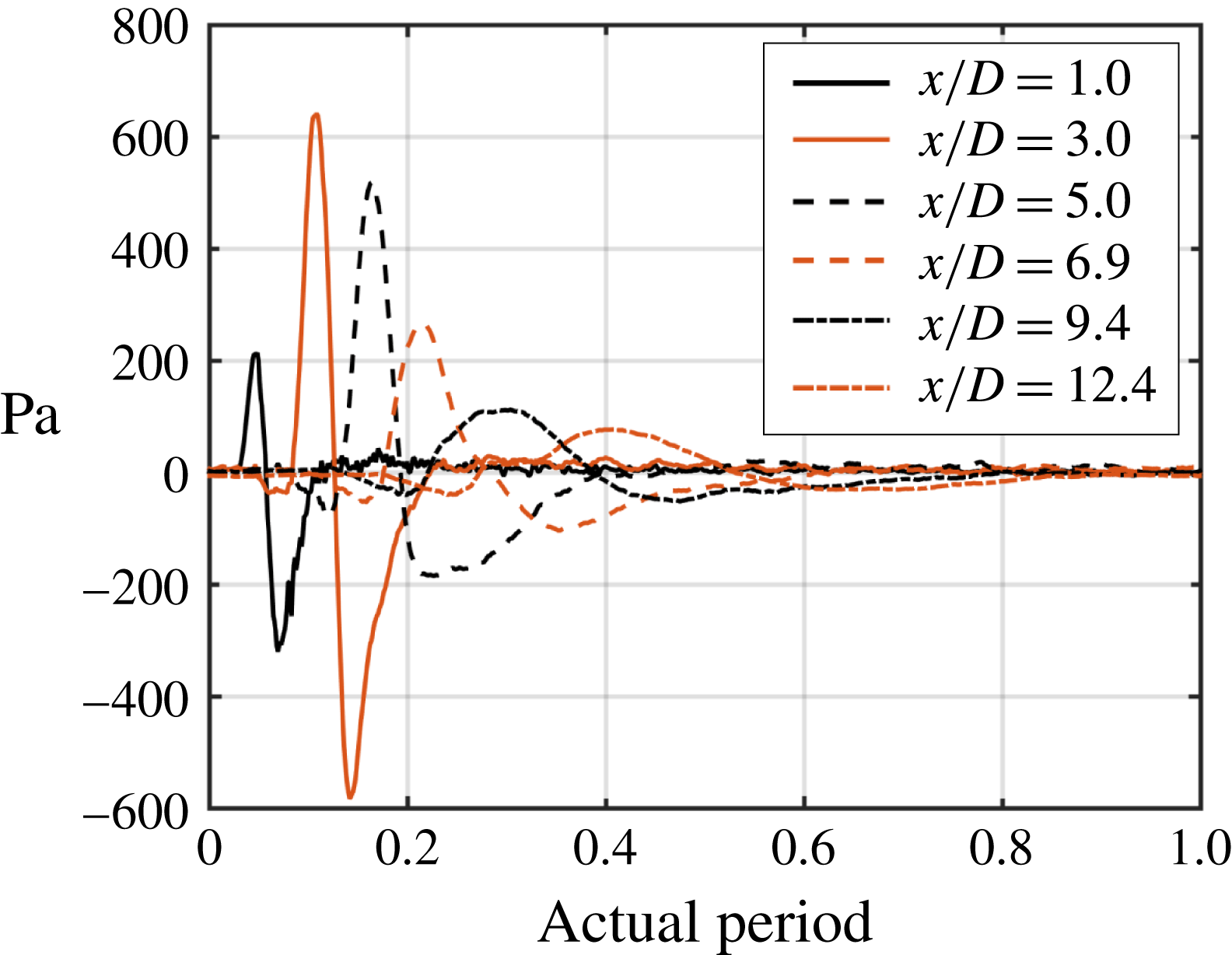
Previous work at the GDTL by Sinha et al. (Reference Sinha, Alkandry, Kearney-Fischer, Samimy and Colonius2012) studied the irrotational near field of a subsonic jet subjected to excitation with plasma actuators by decomposing the instantaneous fluctuating pressure field into a coherent ‘wave’ component (which corresponds to the large-scale structure generated by the excitation) and incoherent residual fluctuations (which correspond to the natural turbulence in the jet). Sinha et al. found that each pulse from the actuators produces a coherent large-scale structure that would grow, saturate, and decay as it advects through the jet shear layer, as demonstrated in figure 2 for excitation Strouhal number (non-dimensional frequency based on jet exit velocity and diameter) of 0.05. In the irrotational near field, the signature of these large-scale structures takes the form of a compact waveform.
Phase-averaged waveforms over a single actuation period for
 $St_{DF}=0.05$
.
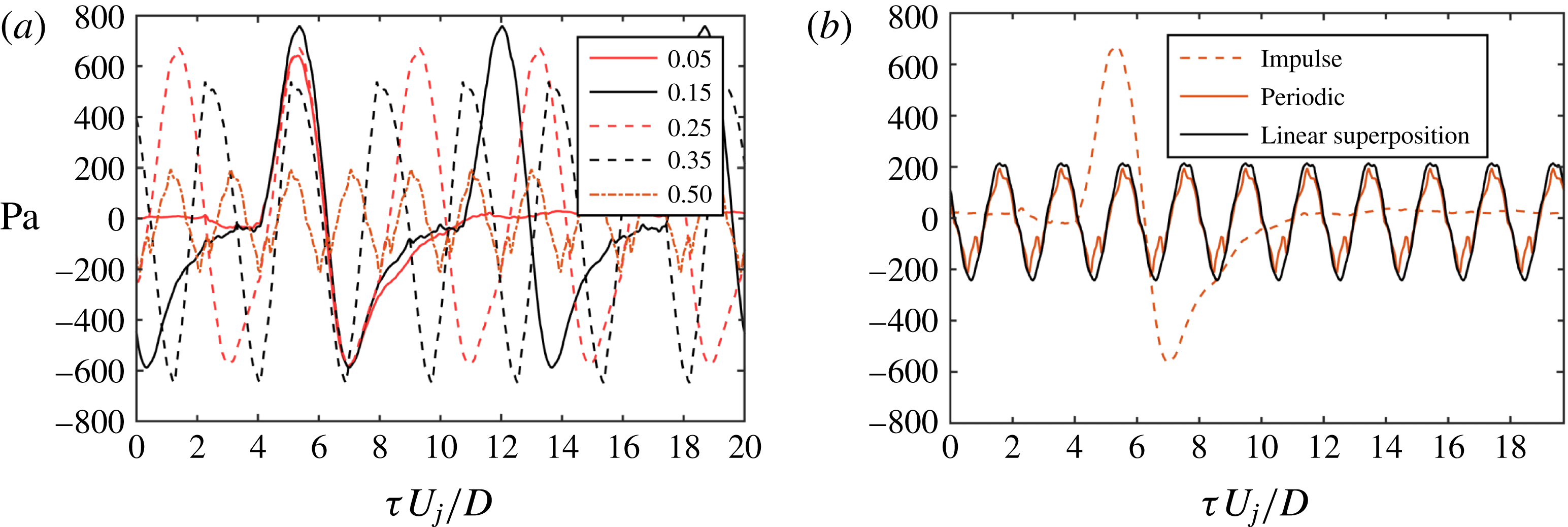
At very low excitation frequencies, the characteristic period of this waveform is much less than the excitation period, and hence, the structures seeded by the excitation do not interact with one another as they evolve downstream. Therefore, their behaviour can be thought of as representing the response of the jet to a single perturbation: the ‘impulse’ response of the jet which is produced by the impulsive excitation by LAFPAs. As the period of actuation approaches the characteristic period of the impulse response, the waveforms extracted by the phase-averaging technique are largely unmodified from that of the impulse response. Above this frequency, significant interaction between the structures is observed, with noticeable modifications to the waveform shape and amplitude. This behaviour can be observed in figure 3(a). As the structures are growing as they advect through the shear layer, the frequency at which the structures begin to interact is dependent on the axial location.
Phase-averaged waveforms for (a) various excitation Strouhal numbers along the first array position at
 $x/D=3,r/D=1.35$
and (b) a linear superposition of the phase-averaged waveform for the impulse excitation (
 $St_{DF}=0.05$
) compared against periodic excitation (
 $St_{DF}=0.50$
).

For a certain range of excitation frequencies (
 $St_{DF}\leqslant 0.50$
at
 $x/D=3$
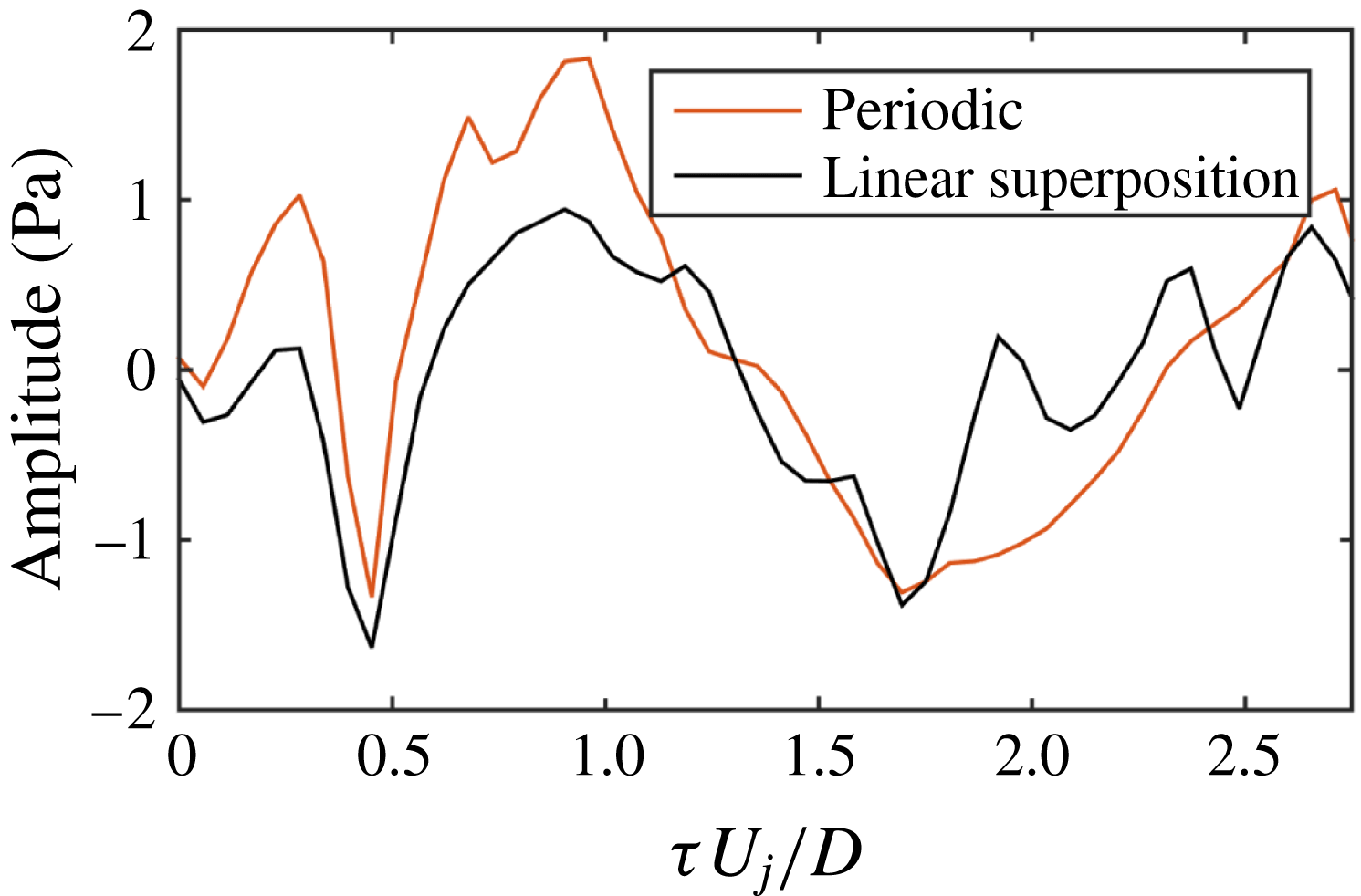
, for example), the structures interact in a quasi-linear manner, insofar as their near-field pressure signatures are concerned. That is, the response of the jet in the irrotational near field could be well predicted by a linear summation of the impulse response of the jet, repeated at the periodic excitation frequency. This concept has been illustrated in figure 3(b), where the periodic response of the jet to excitation with
 $St_{DF}=0.50$
has been reproduced at
 $x/D=3$
. Additionally, a linear superposition of the impulse response for
 $St_{DF}=0.05$
, repeated to match the excitation frequency of
 $St_{DF}=0.50$
, has been overlaid. Upstream of the end of the potential core (
 $x/D\,\simeq \,6$
), the quasi-linear interaction model produces close predictions of the waveform amplitude and shape, despite the significant difference in both peak amplitude and waveform shape between the impulse and periodic responses.
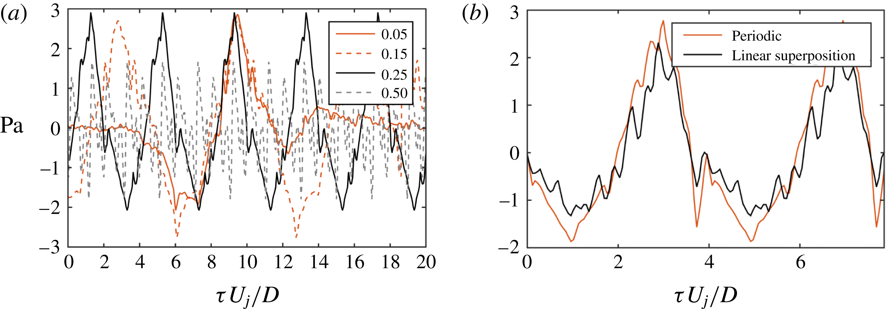
This quasi-linear interaction of the jet response to excitation was found to hold for the acoustic far field as well at aft angles (where the acoustic signal is strongest and is known to correlate well with large-scale structures) (Crawley, Sinha & Samimy Reference Crawley, Sinha and Samimy2015). This can be observed in figure 4(a), where the phase-averaged response of the jet has been plotted for the far-field signal at a polar angle of
 $30^{\circ }$
. For legibility, only a select number of excitation Strouhal numbers have been included. As with the irrotational near field, the acoustic far field exhibits a compact waveform for the lowest excitation Strouhal numbers. At higher
 $St_{DF}$
, a continuous oscillation between sharp expansion and compression waves is again observed, although the amplitude begins to decay above moderate excitation Strouhal numbers.
Phase-averaged waveforms for (a) various excitation Strouhal numbers of the acoustic far field at
 $30^{\circ }$
and (b) a linear superposition of the phase-averaged waveform for the impulse excitation (
 $St_{DF}=0.05$
) compared against periodic excitation (
 $St_{DF}=0.25$
).

As before, a linear superposition of the impulse response can well predict the waveform shape and amplitude at the higher excitation frequencies (figure 4
b), although in this case only up to
 $St_{DF}=0.25$
. From the phase-averaged waveforms alone it is not clear whether this breakdown in the linear superposition model at the higher excitation frequencies is due to nonlinear behaviour or uncertainty in the phase averaging. Results comparing the linear superposition of the impulse response against the measured periodic response at
 $St_{DF}=0.35$
are shown in figure 5. Some similarities may be found in the waveform shape and amplitude, but overall it is clear that the acoustic response of the jet to excitation at
 $St_{DF}=0.35$
is substantially modified from the response at lower frequencies. Although this is hardly conclusive in its own right, this result does suggest either changing or competing acoustic source mechanisms are present in these excited jets. The phase-averaged waveforms were also investigated at polar angles of
 $60^{\circ }$
and
 $90^{\circ }$
; however clear waveforms were not identifiable over the statistical uncertainty inherent in the phase-averaging process. This is likely due to the superdirective character of the acoustic radiation (Crighton & Huerre Reference Crighton and Huerre1990), which renders the amplitude at sideline angles too low to be detectable.
Linear superposition of the phase-averaged impulse response to excitation against the measured periodic response for
 $St_{DF}=0.35$
at the
 $30^{\circ }$
far-field microphone.

3.2 Coherent structures in excited versus natural jets
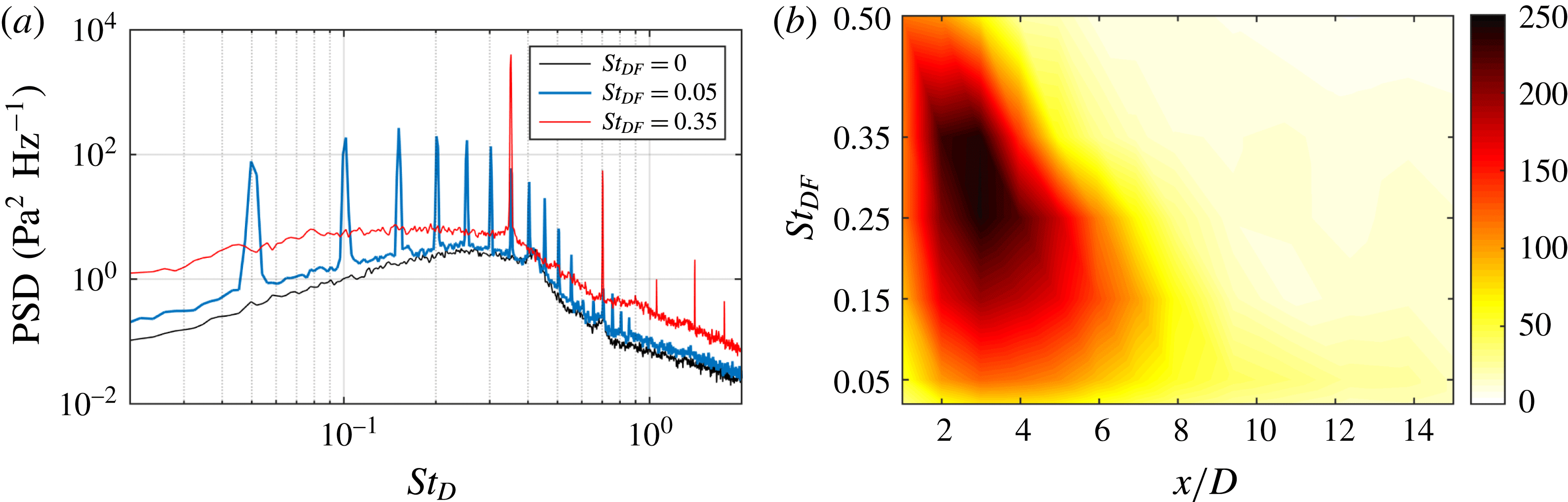
The effect of excitation of natural instabilities in the turbulent jet is to generate highly energetic coherent structures which persist downstream for several length scales, depending upon the excitation Strouhal number. As can be seen by the strong tonal energies observed in the pressure spectra for the excited jets (illustrated in figure 6
a), the near-field signature of these structures contains energy at the fundamental excitation frequency and numerous higher harmonics. The presence of these highly energetic structures can also lead to an amplification of the broadband turbulence over a wide band of frequencies both above and below the fundamental excitation frequency. It also produces a continuous upstream shift in the phase-averaged root-mean-squared peak amplitude, as can be seen in figure 6(b), with the maximum being obtained near
 $St_{DF}\simeq 0.3$
(identified as the jet column Strouhal number in our natural jet). However, the fluctuation intensities in the excited jets saturate much further upstream,
 $x/D\simeq 3$
for
 $St_{DF}\simeq 0.3$
, than those in the natural jet which saturate further downstream near the end of the potential core at
 $x/D\simeq 6$
. In light of this issue, an investigation of the coherent structures in the natural jet and their comparison against those in the excited jet was deemed pertinent to the analysis of the excited structure dynamics. In this section, this will be accomplished by studying the near-field pressure signature of the coherent structures.
Power spectral densities of (a) the raw near-field pressure for the baseline jet and at two excitation Strouhal numbers from the microphone at
 $x/D=3,r/D=1.5$
and (b) root-mean-squared pressure fluctuations (in dB) along the near-field array and as a function of excitation frequency.

It is not possible to use standard phase averaging with the unforced case since the natural turbulent mixing layers, although dominated by Strouhal numbers related to the jet instabilities, contain a broad range of energetic scales with no fixed phase relationship. Therefore it is necessary to use an alternative averaging method in order to extract coherent signatures of the unforced jet structures. A conditional averaging method, specifically wavelet conditioning, was therefore applied to both natural and excited jets. A wavelet decomposition was used as it affords an efficient methodology for analysing intermittent events in a given signal due to the finite energy of its basis functions. This is in contrast to the more standard Fourier decomposition in which continuously oscillating basis functions spread information from a single instance in time across all transform coefficients. The use of the wavelet decomposition has become increasingly common in aeroacoustic research; the reader can refer to Farge (Reference Farge1992) for an overview of the wavelet transform and its applications to turbulence and acoustics.
Wavelet based conditional averaging has been used previously for structure identification in jets and other turbulent flows (Camussi & Guj Reference Camussi and Guj1997, Reference Camussi and Guj1999; Guj & Camussi Reference Guj and Camussi1999; Camussi Reference Camussi2002; Guj, Carley & Camussi Reference Guj, Carley and Camussi2003). The technique educes the signature of coherent structures based on a conditional-average of a turbulent signal using a short-time window centred around highly energetic events identified by the wavelet transform. Identification of the energetic events is accomplished using the local intermittency measure (LIM) (Farge Reference Farge1992), which is the ratio between a local energy of the wavelet coefficient for a specific time and scale and a time-averaged energy at that same scale. The LIM has been demonstrated to be a well-suited indicator for coherent structure identification (Camussi & Guj Reference Camussi and Guj1997). It provides information about the instantaneous fluctuation of energy and by choosing a proper threshold,
 $T$
, it is possible to select a set of times
 $\{\unicode[STIX]{x1D70F}_{i}\}$
corresponding to intermittent energetic events in a signal.
Several methods exist to select the threshold: selecting an arbitrary threshold, using an iterative process to produce a specific value of the flatness factor (kurtosis) or by evaluating the Merit index (Grassucci et al.
Reference Grassucci, Camussi, Jordan and Grizzi2015). In the present study the Merit index method was modified by replacing the usage of a global threshold across all scales with a scale-dependent threshold, which was found iteratively. At each iteration, the coefficient
 $R(T)$
is evaluated:
 $$\begin{eqnarray}R(T)=-\frac{\displaystyle \log \left(\frac{N_{e}}{N_{w}}\right)}{\displaystyle \log \left(\frac{\unicode[STIX]{x1D70E}_{e}}{\unicode[STIX]{x1D70E}_{w}}\right)}.\end{eqnarray}$$
 $N_{e}$
is the number of energetic samples (
 $LIM>T$
),
 $N_{w}$
is the number of incoherent, weak samples (
 $LIM\leqslant T$
) and
 $\unicode[STIX]{x1D70E}_{e}$
and
 $\unicode[STIX]{x1D70E}_{w}$
are the standard deviations for the energetic and weak wavelet coefficients. The threshold is selected as the value maximizing
 $R(T)$
in the same manner as with the original Merit index method (Grassucci et al.
Reference Grassucci, Camussi, Jordan and Grizzi2015).
Conditional averaging (3.2) over the set of times
 $\{\unicode[STIX]{x1D70F}_{i}\}$
is then performed in order to get the coherent structures’ signature as for the phase averaging. At each time location corresponding to a peak of energy, a window
 $W$
of fixed time–length
 $l_{W}$
is selected from the original signal
 $p(t)$
. The conditional-average,
 $\tilde{p}$
is evaluated from this set of windows:
 $$\begin{eqnarray}\tilde{p}^{n}(W)=\frac{1}{N_{e}}\mathop{\sum }_{i=1}^{N_{e}}p^{l}(\unicode[STIX]{x1D709}_{i}),\end{eqnarray}$$
where the superscripts
 $n$
and
 $l$
correspond to the position of the reference signal and of another signal of the array, respectively. Auto-conditioning occurs when the conditional average is performed on a signal
 $p^{n}$
by using its own set of times
 $\tilde{\unicode[STIX]{x1D70F}}^{n}$
, making
 $n=l$
. The subscript
 $s$
corresponds to the scale,
 $\tilde{\unicode[STIX]{x1D70F}}_{s}^{n}$
is the set of corresponding times for a specific scale
 $s$
at which energetic events are occurring, and
 $\{\unicode[STIX]{x1D709}_{i}\}$
is the interval surrounding each peak,
 $\unicode[STIX]{x1D709}_{i}\in [\tilde{t}_{i}-x/2,\tilde{t}_{i}+x/2]$
,
 $\tilde{t}_{i}\in \tilde{\unicode[STIX]{x1D70F}}_{s}^{n}$
. Based on the phase-averaged results, which indicated that a single coherent event could include both positive and negative fluctuations in the pressure domain, only positive pressure peaks were used for identifying energetic events in the conditional average.
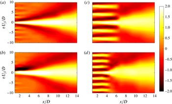
The results for four cases, baseline and
 $St_{DF}=0.05,0.25$
and
 $0.35$
, are presented in figure 7. For the natural jet, the near-field signature of the coherent structures educed by the wavelet autoconditioning takes the form of a strong compression region surrounded by weaker expansion regions on both the leading and trailing edges. As the structure convects downstream, the local time–scale of the fluctuation grows rapidly. This growth in time scale with axial position is expected, given the well-known pattern of growth, saturation, and decay that coherent structures undergo while advecting in a mixing layer and the reduction in convective velocity past the end of the potential core. The amplitude of the compression wave is relatively strong over most of the domain; upstream of
 $x/D=10$
the amplitude of the event is greater than twice the local standard deviation before slowly decaying further downstream.
Wavelet autoconditioned pressure field along the microphone array for (a) the natural jet, (b)
 $St_{DF}=0.05$
, (c)
 $St_{DF}=0.25$
and (d)
 $St_{DF}=0.35$
. The results have been non-dimensionalized by the local standard deviation, and the colour scale is consistent across all plots.

The autoconditioning of the impulse excitation case,
 $St_{DF}=0.05$
, is presented in figure 7(b). General agreement is observed between the coherent signature of the impulsive structures and the natural jet turbulence; they take the form of a strong compression region bookended by expansion regions, the time scales of which increase with axial position. However, noticeable differences are also apparent: the excited structures exhibit a much stronger trailing expansion region than the natural structures, and the decay in amplitude of the expansion and dominant compression regions is much more rapid with axial position. As a result, in the downstream region the energetic event of the impulse excitation case becomes similar in shape to the unforced one, consisting of a central peak and surrounded by two lobes of similar amplitude expansion regions. Results for the periodic excitation cases (
 $St_{DF}=0.25$
and 0.35) are presented in figure 7(c) and figure 7(d), respectively. As with the phase-averaged near-field pressure results for these excitation cases, a repetition of energetic events with the same time scale is observed in the upstream region; rather than one strong compression region and two expansion regions, one compression and one expansion event occurs per excitation cycle. Further downstream however, the continuous oscillations abruptly end, at
 $x/D=6$
for
 $St_{DF}=0.25$
and
 $x/D=4$
for
 $St_{DF}=0.35$
, and the shape of the coherent event begins to revert back to that of the natural jet. As shown in figure 3, the structures generated by the higher-frequency excitation (in this case,
 $St_{DF}\geqslant 0.15$
) begin to interact before they pass through the end of the potential core. This interaction leads to a significant modification of their near-field signature and ultimately the behaviour observed in figure 7.
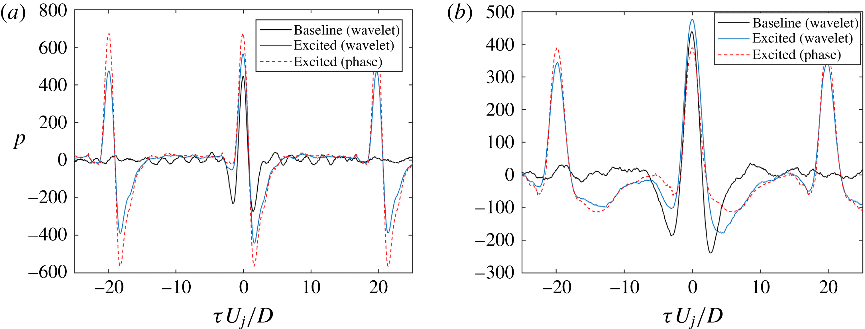
Finally, analysis of the signatures of the excited structure evolution vis-a-vis that of the natural structure evolution was performed. By comparison of the results obtained between the phase averaging and wavelet conditioning for the impulsively excited jet (
 $St_{DF}=0.05$
) and the natural jet (figure 8), several conclusions may be reached. First, while there are small discrepancies between the results obtained from the phase-averaging and wavelet-conditioning methods for the same signal, overall very similar waveforms are produced for the coherent event. As expected, wavelet conditioning is successful in identifying the excited structures over the natural turbulence of the jet, even without being given explicit phase information, and produces analogous results to the phase-averaging method. In the upstream region of the jet, there are differences between the signature of the natural coherent structures educed by wavelet conditioning and those educed by phase averaging in the impulsively excited jet. The expansion region that precedes the primary compression region of the natural structures is nearly non-existent for the excited structures, but the trailing expansion region is more pronounced. However, as the structures convect downstream, near the end of the potential core the coherent waveforms for the natural and excited cases exhibit clear similarity. This indicates that, although the excited structures are far more energetic than those normally found in the jet, the downstream evolution of the natural turbulent structures mirrors (in a statistical sense) that of the intermittent structures generated by the impulse excitation. Therefore, it is reasonable to expect that any acoustic source mechanisms identified near or past the end of the potential core for the excited structures are valid for the natural turbulent structures as well.
Comparison of results for natural and excited (
 $St_{DF}=0.05$
) jet at (a)
 $x/D=3$
and (b)
 $6$
.

3.3 Identifying the acoustic source region
Much of the difficulty in identifying the aeroacoustic source terms revolves around the dissimilar range of scales and fluctuation intensities of the turbulent eddies in the shear layer and the resulting radiated noise. Outside the jet shear layer, in the irrotational near field of the jet, strong hydrodynamic pressure fluctuations associated directly with the passage of coherent structures in the shear layer and their resultant weak acoustic radiation coexist (Arndt et al. Reference Arndt, Long and Glauser1997). Beyond this, in the acoustic far field, the hydrodynamic signature of the coherent structures is non-existent owing to their strong exponential decay with radial distance from the jet mixing layer. As a result, direct identification of pure acoustic waves and their corresponding source events requires decomposition of the near-field pressure into its hydrodynamic and acoustic components.
Coiffet et al. (Reference Coiffet, Jordan, Delville, Gervais and Ricaud2006) demonstrated that the full irrotational near field consisted as a linear superposition of hydrodynamic and acoustic fields, with very weak nonlinearities; this led subsequent researchers to propose linear filters to decompose the individual components. Tinney & Jordan (Reference Tinney and Jordan2008) proposed using a two-dimensional Fourier transform to decompose the near field, arguing that in a transonic jet in which the large-scale structures are convecting subsonically, a demarcation of the hydrodynamic and acoustic energy fields can be made by phase velocity. This is because the hydrodynamic pressure fluctuations will be aligned with the jet axis, and travelling subsonically with respect to the ambient speed of sound. Acoustic pressure fluctuations will impinge on the linear microphone array at oblique angles, and therefore will appear as having either sonic or supersonic phase velocity, based on the source location relative to the microphone array. Therefore, a demarcation between the hydrodynamic and acoustic energy components should be readily identifiable about the sonic wavenumber,
 $k_{a}=\unicode[STIX]{x1D714}/a_{\infty }$
. Decomposition of the irrotational near-field pressure is therefore straightforward in Fourier space. Grizzi & Camussi (Reference Grizzi and Camussi2012) took a different approach and utilized a discrete wavelet transform at individual spatial locations in order to decompose the fields based on an energy cutoff. The energy threshold was set iteratively, using analysis of two-point correlations of the acoustic and hydrodynamic components between two microphones, in order to ensure that realistic phase velocities for the components were met.
However, there is also a great drawback associated with Fourier analysis: while it analyses a given signal at a distinct frequency, local information for a given event is spread over all spectral coefficients. This is due to the fact that the basis functions used by the Fourier transform oscillate indefinitely. For a signal composed of completely random fluctuations this is not an issue, however it has become increasingly clear that the jet noise phenomenon is dominated by large-scale structures, the production of which is statistically correlated (Kearney-Fischer et al. Reference Kearney-Fischer, Sinha and Samimy2013). Transient events, such as intermittency or the spatial and temporal modulation of a wavepacket, have been shown to be important in the noise generation process. It was for this reason that a continuous spatio-temporal wavelet filter, based on the work of Antoine et al. (Reference Antoine, Murenzi, Vandergheynst and Ali2004) and Kikuchi & Wang (Reference Kikuchi and Wang2010), was instead used in the current work to decompose the acoustic and hydrodynamic near fields based on phase velocity. It has been shown that by using a temporally/spatially localized fluctuation as a basis, the wavelet transform compresses the information in a turbulent field much more efficiently (and accurately) than the Fourier transform (Farge Reference Farge1992). This is particularly beneficial for the current work, where the spatial resolution is low due to the limited number of microphones used.
The spatio-temporal wavelet filter is quite similar in concept to that of Tinney & Jordan (Reference Tinney and Jordan2008). It proposes separating the acoustic and hydrodynamic near-field pressure components of a jet with subsonically convecting eddies according to measured phase velocity from a linear array of microphones outside the jet shear layer. In this case the filtering function is derived from the commonly used Morlet wavelet. As with the Fourier filter, the decomposition is performed by transforming the pressure traces from the near-field microphones in both space and time using the filter function, and the individual components are then recovered by inverse transformation over a subset of phase velocities (either subsonic or supersonic). A more detailed explanation of the spatio-temporal wavelet transform, the justification for its use in decomposing the near-field pressure, and validation of the methodology using the current database can be found in Crawley, Kuo, & Samimy (Reference Crawley, Kuo and Samimy2016).
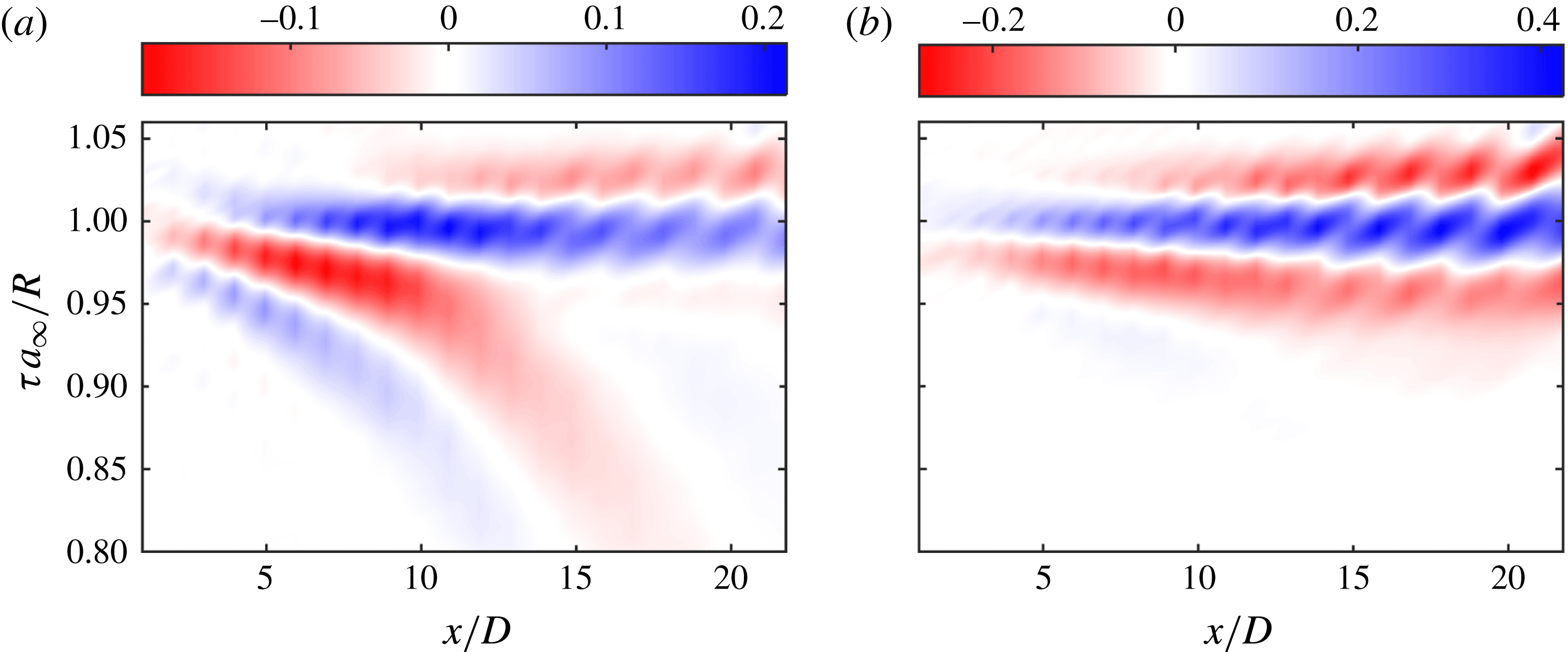
By decomposing the irrotational near-field pressure, the relationship between the near and far field can be more easily elucidated. Two-point correlations were computed using both the full near-field and the acoustic near-field component, between each microphone in the near field and the far-field microphone at
 $30^{\circ }$
; results can be found in figure 9. It shows distinct regions of positive and negative correlation spanning several jet diameters and flow time scales. The time lag,
 $\unicode[STIX]{x1D70F}$
, in the figures has been non-dimensionalized by the ambient speed of sound,
 $a_{\infty }$
and
 $R$
, the distance from each near-field microphone to the far-field microphone (note that this results in an ordinate that is scaled separately along the abscissa, due to the dependence of the axial position on
 $R$
).
Normalized two-point correlations for the natural jet between the near field and the far field at
 $30^{\circ }$
for (a) the full near-field pressure and (b) the acoustic component only.

Near the jet shear layer (figure 9
a) four distinct correlation regions can be observed: two positive and two negative; one strong and one weak for each. The first correlation regions, the strong negative and weak positive, are noticeable beginning at the most upstream microphone and reach their peak values around
 $5<x/D<10$
, decaying significantly beyond that. By tracing the local peaks for these individual correlation regions, the propagation velocity for the physical phenomena can be estimated from the shift in
 $\unicode[STIX]{x1D70F}$
as a function of
 $x$
. The slopes of these regions indicate propagation velocities noticeably below the sonic velocity. In the upstream region, they roughly match with the measured convective velocity of the large-scale structures (
 $U_{c}\simeq 0.7U_{j}$
(Crawley et al.
Reference Crawley, Sinha and Samimy2015)) in the upstream region of the jet, and slowly decelerate downstream. Similar behaviour was observed by Bogey & Bailly (Reference Bogey and Bailly2007), which noted that two-point correlations between the flow field and acoustic near field in a simulated jet produced strong positive correlation regions which peaked at the end of the potential core and followed the convection of the large-scale structures. Conversely, the strong-positive and weak-negative correlation regions exhibit propagation velocities that match well with the ambient speed of sound. The distinctly different propagation velocities of the two pairs of correlation regions indicate that these correspond to different physical phenomena. The strong-negative and weak-positive correlation regions observed near the jet shear layer are associated with the large-scale structures themselves, rather than acoustic phenomena. This relationship becomes even more clear when just the acoustic component of the near field is considered, rather than the full irrotational near field. The correlation regions with subsonic propagation velocities (figure 9
b) have entirely disappeared, and instead, a single positive correlation region corresponding to sonically propagating waves exists over the entire domain.
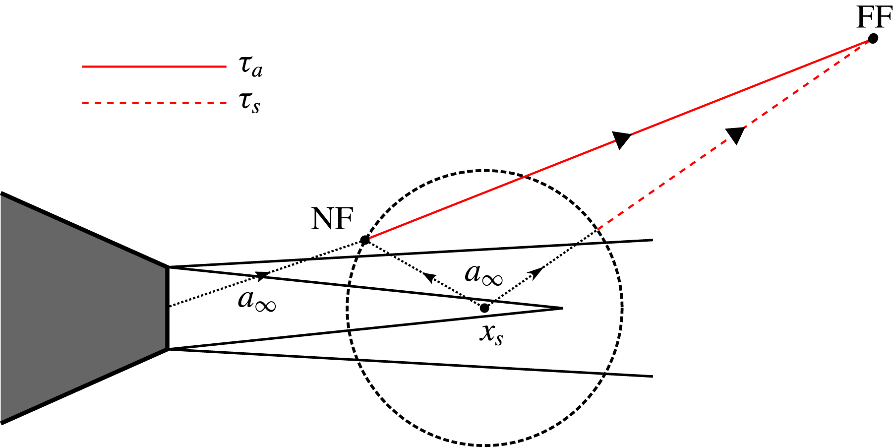
The correlations of the decomposed near field can be used to identify the acoustic source region, in a rough sense, by comparing the time lag at which the greatest correlation is achieved against expected times-of-arrival for different propagation paths. A schematic of these propagation paths is provided in figure 10. The first expected time of arrival,
 $\unicode[STIX]{x1D70F}_{a}$
, corresponds to the expected time lag for an acoustic wave travelling directly from the noise source to the near-field microphone and on to the far-field microphone and hence, the noise source region lies along the axis created by the near-field and far-field microphones. Another expected time of arrival can be constructed by assuming the source region is stationary in space; from simple geometric considerations of the distance from the assumed source region to the near-field and far-field microphones, the time lag,
 $\unicode[STIX]{x1D70F}_{s}$
, between the arrival of an acoustic wave at both microphones can be computed. The stationary source region is not known a priori, but is set by the author subsequent to the computation of the two-point correlations. For this analysis, the results from the
 $30^{\circ }$
far-field microphone were used exclusively. This is because the correlations between the near-field and sideline microphones (
 $60^{\circ }$
and
 $90^{\circ }$
) were very weak.
For simplicity, density and convection effects on the acoustic wave as it travels through the jet shear layer have been neglected in this analysis. By necessity, it has been assumed that the acoustic radiation in the jet is dominated by
 $m=0$
azimuthal Fourier mode (the near-field and far-field microphone arrays are not at the same azimuthal angle with respect to the nozzle). This assumption is easily justified in the excited jets, where the actuators have been fired in phase. While the near-field pressure and acoustic radiation towards aft polar angles in a natural, high Reynolds number jet is a combination of numerous azimuthal Fourier modes, previous researchers have found these fields to be dominated by the axisymmetric mode (Juvé et al.
Reference Juvé, Sunyach and Comte-Bellot1979; Arndt et al.
Reference Arndt, Long and Glauser1997; Hall et al.
Reference Hall, Pinier, Hall and Glauser2006; Kœnig et al.
Reference Kœnig, Cavalieri, Jordan, Delville, Gervais and Papamoschou2013).
Expected times of arrival for on-axis acoustic propagation,
 $\unicode[STIX]{x1D70F}_{a}$
, and off-axis acoustic propagation,
 $\unicode[STIX]{x1D70F}_{s}$
from a stationary source region centred at
 $x_{s}$
.

Here, the acoustic source region was assumed to be located at
 $x_{s}/D=4$
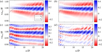
, which is just upstream of the end of the potential core in the unforced jet. (Note that this analysis is not meant to imply that the source region is located at a specific fixed point, it is merely a convenient way of understanding the propagation paths.) The behaviour of the excited jets shown in figure 11 is similar to the natural jet behaviour; note that due to numerical discrepancies at the domain boundaries (see Torrence & Compo (Reference Torrence and Compo1998) for a discussion of the ‘cone of influence’ of wavelet coefficients and the effect thereof), the correlation values have been truncated at the most upstream and downstream microphones. For the impulsively excited jet, nearly identical correlation regions are observed between the excited and natural jet; in the periodically excited jet continuous oscillations occur due to the similarity of continuously and periodically generated large-scale structures and resultant acoustic radiation. In the upstream region of the jet, the peaks of the positive correlation region match
 $\unicode[STIX]{x1D70F}_{a}$
nearly exactly. In the downstream region,
 $\unicode[STIX]{x1D70F}_{a}$
begins to increasingly over-predict the time lag for the maximum correlation. On the other hand,
 $\unicode[STIX]{x1D70F}_{s}$
tracks the time lags for the peak correlation consistently over the downstream region, but not the upstream region. The results found here indicate that the dominant acoustic radiation reaching the far-field aft angles is being generated over an extended region of the jet mixing layer, near and upstream of the end of the potential core, for both natural and excited jets. This is similar to the findings of other researchers, who have suggested that the acoustic source region lies just downstream of the end of the potential core (Hileman et al.
Reference Hileman, Thurow, Caraballo and Samimy2005). It should be clarified here though, that the interpretation of these results is not meant to suggest that only trivial levels of noise are generated outside of this apparent noise source region, just that the dominant radiation is produced near the end of the potential core in a time-averaged sense.
Normalized two-point correlations between the acoustic component of the near field and the far field at
 $30^{\circ }$
for microphone array position starting at
 $x/D=1,r/D=1.2$
for (a) the natural jet, (b)
 $St_{DF}=0.05$
, (c)
 $St_{DF}=0.25$
and (d)
 $St_{DF}=0.35$
.

These results should not be interpreted as indicating that the source mechanisms are necessarily consistent for all excitation frequencies. For the lower-frequency periodic excitation (
 $St_{DF}\leqslant 0.25$
), the consistency in the far-field signature (figure 4
b) coupled with the consistency in the apparent source region is suggestive of a consistent dominant source mechanism. In contrast, the inconsistency in the far-field response of the jet to higher-frequency periodic excitation (
 $St_{DF}\geqslant 0.35$
, figure 5) is suggestive of a change in the dominant source mechanism, just one that is associated with the vortex dynamics in the jet shear layer upstream of the end of the potential core. It should also be noted that the peak correlation values between the acoustic near field and the far field are significantly lower (though certainly non-negligible) in the periodic excitation cases (
 ${\sim}0.2{-}0.3$
in the periodic cases versus
 ${\sim}0.4$
in the natural jet and impulse excitation), suggesting a decaying coherence in the source mechanisms at these frequencies. It should be kept in mind that the analysis described in this section is fairly simplistic in it’s assumptions (stationary point source and no convection or diffraction effects), and hence was not meant to determine the exact source region; it is meant as a rough outline. From the current results alone, the significance of this estimated source region is not entirely clear. In § 4 the time-resolved velocity field will be explored in detail to better elucidate the structure dynamics, with a particular focus on the region just upstream of the end of the potential core.
A special note on the differences concerning the results presented in figure 11 and those presented by Crawley et al. (Reference Crawley, Sinha and Samimy2015) is warranted here. In that paper, the more simple Fourier filter was used to decompose the irrotational near field; processing artefacts were noted and a parametric study was attempted to minimize their impact. In the resulting two-point correlations of the decomposed acoustic field, a shift in the apparent source region was noted to coincide with the shift of the peak pressure fluctuations measured just outside the shear layer (higher-frequency excitation cases saturating further upstream near the nozzle exit). Because this behaviour was observed across the entire range of filter parameters used, it was assumed to be representative of the true physical behaviour and not a numerical artefact. Of course, this assumption precludes the possibility that the entire parameter space produced similar numerical artefacts. It was found that the Fourier filter has a tendency to allow energy leakage from the hydrodynamic field into the acoustic, particularly at low frequencies. Since it has already been observed that the hydrodynamic signature of the large-scale structures can linearly correlate to the acoustic emission, a potential consequence of this leakage is correlation regions which instead point to the region of high hydrodynamic energy – i.e. the saturation point of the near-field pressure fluctuations. The analysis of Crawley et al. (Reference Crawley, Kuo and Samimy2016) demonstrated that wavelet filter is far more robust to energy leakage and numerical artefacts, and as such the authors is inclined to lend more credence to the results presented herein.
4 Vortex dynamics in a turbulent mixing layer
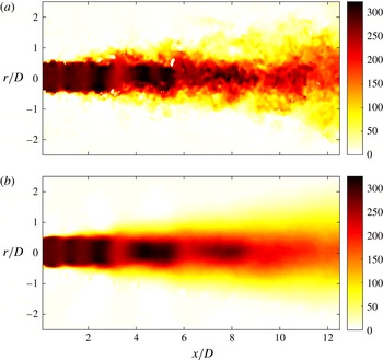
Analysis of the evolution, interaction and disintegration of the large-scale structures, and ultimately the noise generated by these processes, is greatly aided by the acquisition of time-resolved flow-field measurements. Unfortunately, directly acquiring time-resolved velocity fields for the jet currently under study is simply not possible due to the combination of a large domain of interest (
 $0\leqslant x/D\lesssim 12,0\leqslant r/D\lesssim 3$
) and high characteristic frequencies of the order of several kHz. Full-field, high-fidelity measurement techniques capable of this required repetition rate were not available to the researchers. An indirect method was therefore developed to estimate the evolution of the large-scale structures. Phase locking of a data acquisition system to a reference signal (such as an actuator or a naturally occurring resonance tone) is a common experimental technique, and was initially considered for the present work. However, interpretation of the results is highly dependent on the acquired phase resolution. Acquiring a high number of phases is time consuming and tedious, while acquiring a lower number of phases risks missing higher-frequency vortex dynamics. Clearly, a more efficient data acquisition method is needed.
4.1 Stochastic estimation
The current work heavily relies on the methodology of Tinney, Eukeiley & Glauser (Reference Tinney, Eukeiley and Glauser2008) and Sinha, Serrani & Samimy (Reference Sinha, Serrani and Samimy2010) in order to estimate the two-component time-resolved velocity field on a streamwise planar slice of the jet. The computational methodology by which the stochastic estimation is performed has been modified, however. Complementary stochastic estimation is used, due to its significantly lower computational time as well as theorized improvement in accuracy (Taylor & Glauser Reference Taylor and Glauser2004). The estimated velocity fields produced by linear stochastic estimation (LSE) were projected onto the proper orthogonal decomposition (POD) eigenfunctions (computed from the random, non-time-resolved velocity fields) to produce an estimate of the time-dependent POD coefficients, which can then be used to reconstruct low-order representations of the estimated random velocity field. Multiple time delays are incorporated, as this has been found to significantly improve the accuracy of the reconstructions for many flow regimes (Ewing & Citriniti Reference Ewing, Citriniti, Sorensen, Hopfinger and Aubry1997; Tinney et al. Reference Tinney, Coiffet, Delville, Hall, Jordan and Glauser2006, Reference Tinney, Eukeiley and Glauser2008; Durgesh & Naughton Reference Durgesh and Naughton2010). Instead of performing the stochastic estimation using either linear or higher-order cross-correlations (or cross-spectra), the conditional mapping between the near-field pressure and the POD modal coefficients was generated by an artificial neural network (ANN). ANNs were chosen over the more traditional cross-correlations due to their simplicity compared to high-order methods as well as their demonstrated ability to model nonlinear processes in turbulent flows (Lasagna et al. Reference Lasagna, Fronges, Orazi and Iuso2015).
A feedforward network structure was used; it was comprised of an input layer, to which near-field pressure traces were supplied, a single hidden layer containing 32 neurons, and an output layer which produced estimates of the time-varying POD coefficients. The hidden and output layers were fully connected, and the modified logistic function (hyperbolic tangent) was used as the activation function. The pressure traces were centred around the acquisition of a PIV image group, and were downsampled to 100 kHz in order to approximate the frequency response of the microphones. The record time supplied for each training block was
 $\pm 2.56~\text{ms}$
; this was determined by estimating the time delay for a large-scale structure to convect through the experimental domain (the convective velocity of the large-scale structures was conservatively estimated as
 $U_{c}\simeq 0.5U_{j}$
).
POD modes and time-varying coefficients were computed from the velocity fields using the method of snapshots (Sirovich Reference Sirovich1987); the kernel was defined as the two-component turbulent kinetic energy. The instantaneous velocity fields were not preprocessed prior to the decomposition (that is, missing or spurious vectors were not replaced or interpolated). As experimental noise in the velocity fields is completely uncorrelated to the near-field measurements, it is filtered out by the stochastic estimation and hence preprocessing is unnecessary. In this work, the coefficients for every POD mode were estimated, rather than just the most energetic modes, for two reasons. First, it is not guaranteed that an individual POD mode corresponds to a physically distinct turbulent flow structure or event – an event may be broken up into multiple POD modes of varying energy levels. Secondly, the most energetic POD mode is not necessarily the most relevant mode for the acoustic generation process (Jordan et al. (Reference Jordan, Schlegel, Stalnov, Noack and Tinney2007) proposed a modification to the standard POD kernel in order to mitigate this issue). The second issue is that highly relevant dynamic processes may contain little energy as defined by the standard POD kernel (Noack et al. Reference Noack, Afanasiev, Morzynski, Tadmor and Thiele2008); this has led researchers to propose alternative methods for extracting dynamic features of turbulent flows (Schmid Reference Schmid2010). Even though the network is estimating even the least-energetic modes, the current method is far more computationally efficient than directly estimating the velocity fields themselves.
Network training was accomplished via the standard backpropagation method (Haykin Reference Haykin1994), which approximates the error surface of the cost function using first-order derivatives; the error ‘propagates’ backwards from the output neurons to the hidden neurons and the synaptic weights at each neuron are updated to identify the minimum of the cost function using gradient descent. The cost function was defined as the mean-squared-error between the predicted and measured expansion coefficients for a given PIV image group. Training of the network was performed using the roughly 1500 ensemble pressure–velocity blocks of data (a few PIV images in each set had to be discarded due to laser misfires); synaptic weights were updated based on the average of all blocks (batch processing) using a constant learning rate. In order to prevent overfitting, the training was limited to 5000 epochs. Validation of the stochastic estimation produced by the neural network is demonstrated in the appendix.
4.2 Large-scale structure disintegration
Hileman et al. (Reference Hileman, Thurow, Caraballo and Samimy2005) investigated the evolution and interactions of large-scale structures and ultimately how these relate to the noise generation process in a supersonic, ideally expanded jet by combining time-resolved flow visualizations with a three-dimensional microphone array. Their results showed that the dominant noise was generated near the end of the potential core, in the region where the shear layers merged. Large-amplitude, highly intermittent acoustic events were found to be associated with a fluctuation in the length of the potential core, which the authors ultimately speculated was related to the passage and finally the rapid disintegration of large-scale coherent structures just downstream of the end of the potential core. The dynamics of the large-scale structures in this region, namely the structure disintegration, are therefore of particular concern to the current work.
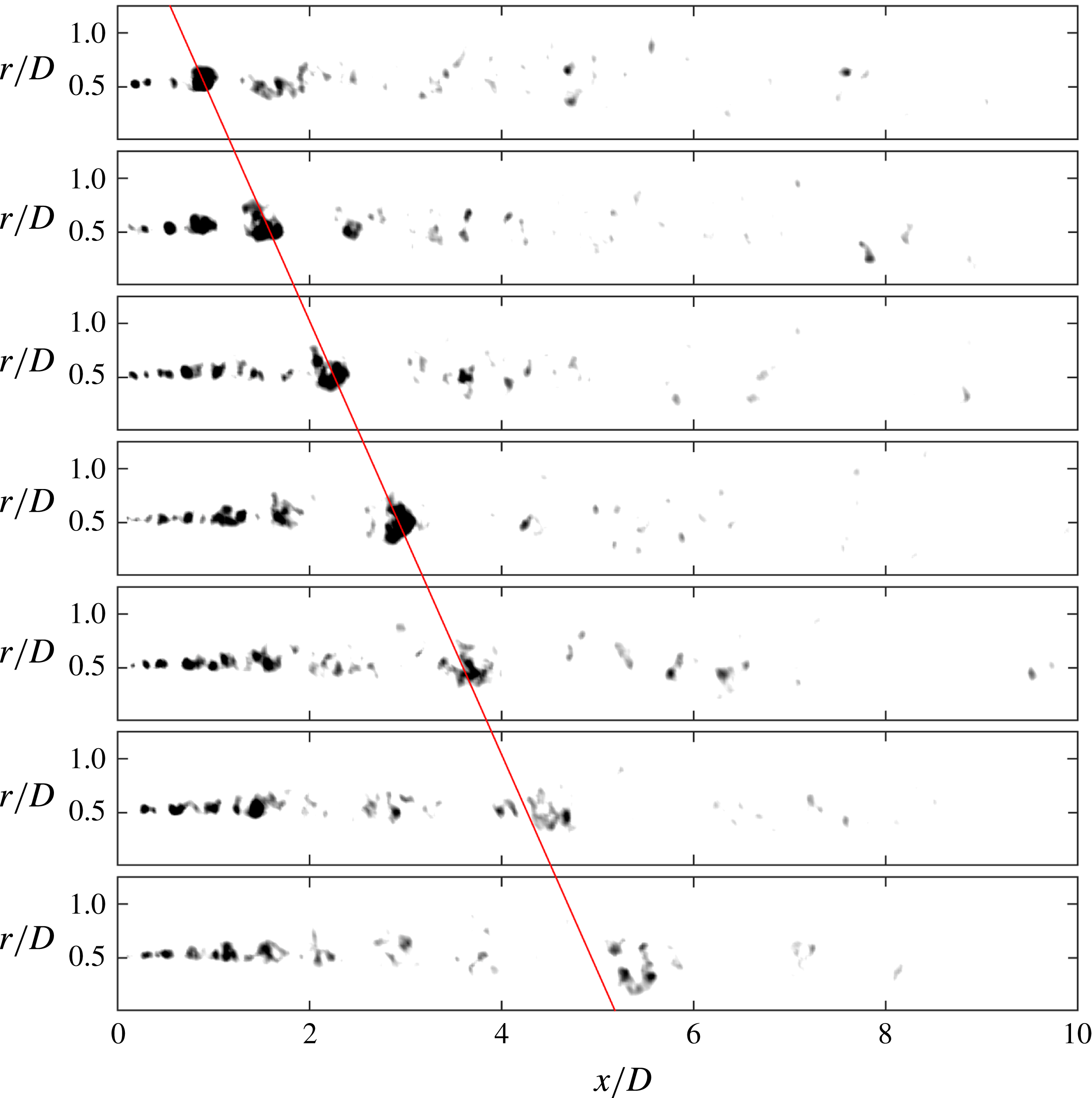
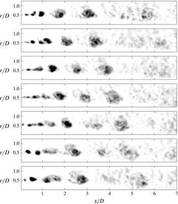
Vortex identification was performed by computing the swirling strength at each instance in the estimated velocity field. The evolution of the impulsively excited (
 $St_{DF}=0.05$
) vortex ring has been tracked in figure 12. For ease of visualization, a two-dimensional, five-point boxcar filter was applied to the estimated velocity fields prior to computing the swirling strength, and the results have been phase averaged based on the recorded LAFPA trigger signal over roughly 30 excitation periods. Lastly, a solid red line has been overlaid to approximately match the convective velocity of the structures. Only a select number of phases are shown here, as a significant amount of dead time between excitations occurs due to the mismatch in the spatial and temporal characteristic frequencies of the large-scale structures.
Evolution of the independent vortex ring (impulse excitation at
 $St_{DF}=0.05$
), as visualized using swirling strength. Images are shown at constant phase steps of roughly
 $\unicode[STIX]{x03C0}/8$
, starting with a phase of
 $\unicode[STIX]{x03C0}/4$
.

As already known from prior experiments at the GDTL (Kearney-Fischer et al.
Reference Kearney-Fischer, Kim and Samimy2009), the excitation produces a strong roll up of toroidal structures in the near-nozzle region; in the present case the large-scale structure generated by the excitation is clearly discernible over the background turbulence (and experimental/computational noise) by
 $x/D\simeq 1$
. The rapid growth of the vortex slows by
 $x/D\simeq 1.5$
and it advects downstream relatively unchanged until
 $x/D\simeq 4$
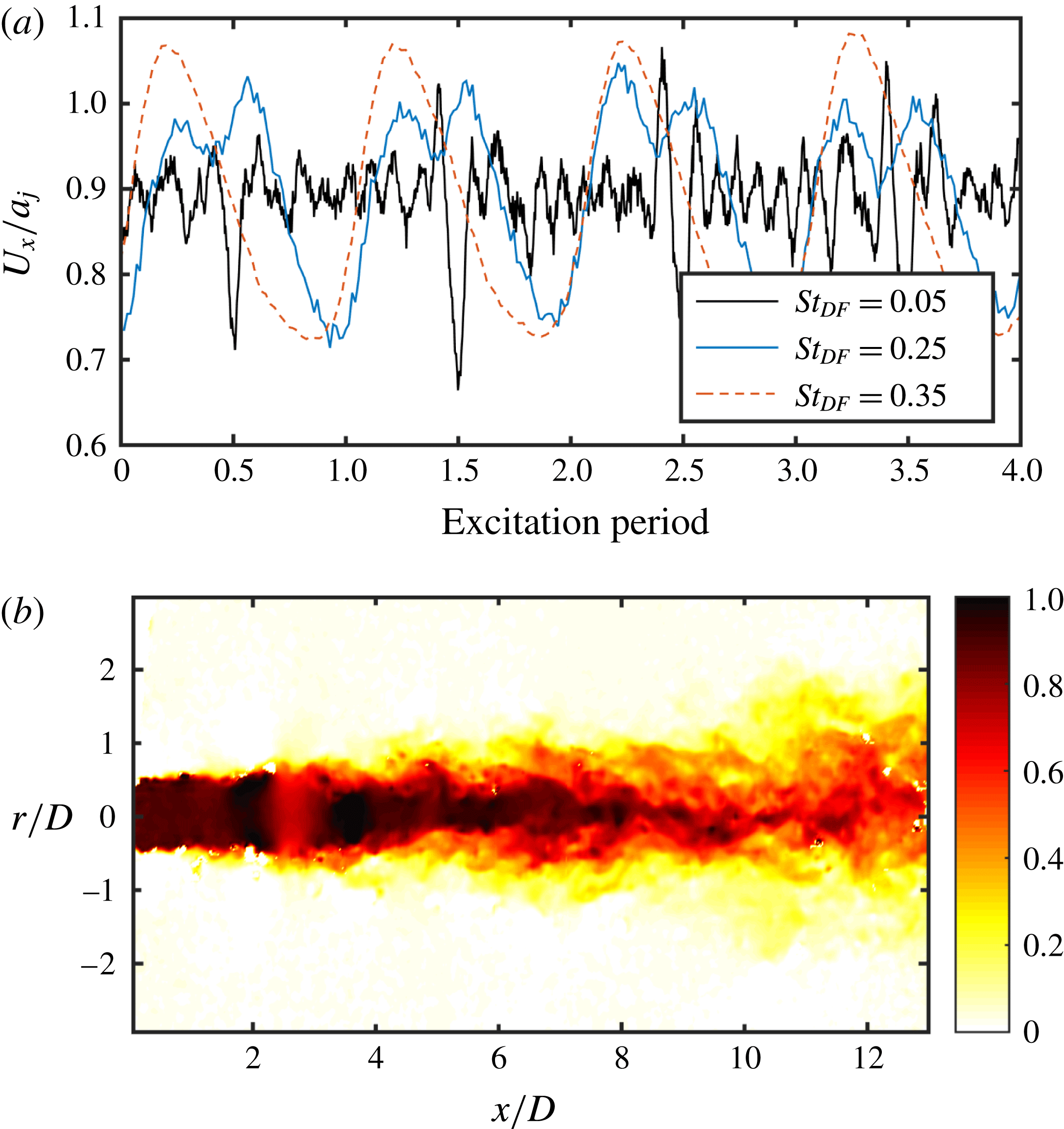
. It is at this point that the vortex undergoes rapid disintegration, yielding smaller-scale, less coherent structures as it passes through the end of the potential core. Accompanying the passage of the structure is a large amplitude oscillation in the axial velocity, which reaches into the potential core to the jet centreline, consistent with the radial profile of axisymmetric instability waves in linear stability analysis (Michalke Reference Michalke1965). As shown in figure 13, the vortical structures are characterized by large velocity deficit, which is preceded by a large acceleration of the fluid that often crosses the sonic threshold as the vortex begins to disintegrate. It was surprising to see such a strong axial acceleration, however this same axial acceleration can also be found in the raw PIV snapshots that have not been post-processed by complementary stochastic estimation (note the coherent region of supersonic velocity just upstream of
 $x/D=4$
in figure 13
b). An acceleration of the less-coherent structures can also be observed in figure 12, as the small eddies are located further downstream in the final frames than they would be if following a constant convective velocity (as denoted by the red line overlain on the frames). As discussed by Tam, Golebiowski & Seiner (Reference Tam, Golebiowski and Seiner1996), the aeroacoustic efficiency of structures increases with Mach number and envelope modulation. Therefore, the twin effects of rapid disintegration (i.e. rapid envelope modulation) and acceleration around
 $x/D\simeq 4$
would greatly enhance the acoustic efficiency from the vortex. This potentially explains why the region in which the turbulent structure rapidly disintegrates appears to dominate versus the region in which the turbulent structure rapidly grows in terms of the noise emission per the results of § 3.
Fluctuations associated with the passage of large-scale structures in (a) the axial velocity along the jet centreline at
 $x/D=4$
and (b) an arbitrary raw PIV snapshot displaying Mach number contours, showing similar behaviour for the
 $St_{DF}=0.05$
jet.

4.3 Coherent structure merging
In the simulated subsonic shear layer of Wei & Freund (Reference Wei and Freund2006), optimized control for noise mitigation using generalized actuation was implemented using the adjoint perturbation method. The methodology was able to produce a significant reduction in the emitted noise, although the exact mechanism by which this was accomplished was not immediately clear, even in this highly simplified flow (two-dimensional shear layer). In Cavalieri et al. (Reference Cavalieri, Jordan, Gervais, Wei and Freund2010) the same numerical database was investigated with a specific focus on identifying intermittent events related to the noise generation process. It was found that control achieved the majority of the sound reduction by suppressing a single, triple-vortex interaction, thereby modifying the flow and preventing the generation of high-amplitude peaks in the acoustic field. The experiments of Kibens (Reference Kibens1980) also identified vortex merging as a prominent noise source in a (low) subsonic jet. With this in mind, the evolution of the vortices in the periodically excited jets was analysed.
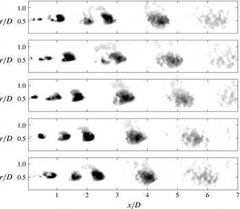
Figure 14 illustrates a complete excitation period for the
 $St_{DF}=0.25$
excited jet; as before, the velocity fields were smoothed prior to computation of the swirling strength, and the results have been phase averaged over approximately 150 phases. Previous analysis of the near-field had used two-point correlations between subsequent microphones in order to estimate the convective velocity of the large-scale structures; based on the time-lag for the maximum correlation value, the convective velocity was estimated as
 $U_{c}\simeq 0.7U_{j}$
. However, the analysis of Speth (Reference Speth2015) in a simulated Mach 0.9 unheated jet found that this method over-predicted the convective velocity; for example, near the end of the potential core two-point correlations in the irrotational near-field produced an estimate of
 $U_{c}\simeq 0.67U_{j}$
whereas correlations in the flow-field produced an estimate of
 $U_{c}\simeq 0.64U_{j}$
. Essentially, the energy of the acoustic field in the irrotational near field although small, is non-trivial, and as a result the much higher propagation velocity for the acoustic energy skews the convective velocity estimate to slightly higher values. Using two-point correlations of the hydrodynamic component of the near field measured by subsequent microphones, the convective velocity was estimated as
 $U_{c}\simeq 0.54U_{j}$
near the nozzle exit and
 $U_{c}\simeq 0.65U_{j}$
near the end of the potential core. Based on these values, the vortex spacing is expected to be
 $\simeq 2.6D$
near the end of the potential core.
Evolution of the periodic vortex ring (
 $St_{DF}=0.25$
), as visualized using swirling strength. One complete actuation period is shown.

The excitation produces a periodic roll-up of large-scale structures, the spacings of which, in the downstream region near the end of the potential core, roughly match with the vortex spacing for this frequency (see frame 1 in figure 14). However, in the upstream region (
 $x/D<2$
) the vortex spacing halves – the LAFPA excitation is in fact producing structures with a frequency associated with the most unstable shear layer frequency, which is significantly higher than the jet column mode frequency. This behaviour can be explained if the specifics of LAFPA actuation are considered with respect to the well-known shear layer instability characteristics. Unlike many other actuators used previously for flow control in low speed and low Reynolds number flows, the perturbation generated by the LAFPAs is non-sinusoidal and comprised of many higher harmonics. These harmonics, although of lower amplitude than the fundamental excitation frequency, couple to the flow and excite the shear layer instability, which is most unstable at frequencies much higher than the excitation frequencies used in this work. Therefore, the structures initially formed by the excitation are associated with harmonics of the excitation frequency. Hence, it is only after merging (or successive mergings) that the passage frequency of the large-scale structures matches the fundamental excitation frequency.
In frame 2, the two structures at
 $x/D=1$
are beginning to merge. The trailing structure is inducted into the preceding structure, and by
 $x/D\simeq 3$
the merging process is complete. As the resultant structure convects downstream, the beginning of the breakdown of the vortex is witnessed near
 $x/D\simeq 4$
, similar to the results of the impulsively excited vortex ring and an acceleration of the centreline velocity to slightly supersonic speeds (figure 13
a). Here however, a secondary interaction between structures appears to be occurring, most visibly in frames 5–7. It appears that a second merging process is commencing here, however the vortex disintegrate before the trailing vortex can be inducted into the leading vortex. As the vortex at
 $x/D\simeq 4.5$
is breaking down, the trailing vortex breaks down as well: much more abruptly than the leading vortex. At this point the spacing of structures matches the excitation period. As the cycle is repeated (beginning again at frame 1), these two vortices (or more accurately, the less coherent, higher-order remnants of them) are no longer individually distinguishable.
Recall that the far-field response of the jet to periodic excitation at
 $St_{DF}=0.35$
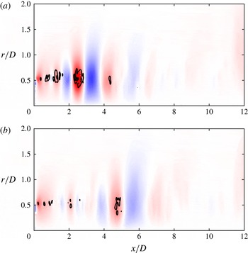
could not be reproduced accurately using a linear superposition of the impulse response (figure 5). The vortex dynamics that this excitation frequency produces may thus serve as an insightful contrast for understanding the noise generation phenomena. A complete excitation cycle for
 $St_{DF}=0.35$
has been visualized in figure 15. In this case, two merging processes are now clearly evident. The first begins just downstream of the nozzle exit, and completes by
 $x/D\simeq 1.5$
(frames 3 and 4); the second begins at
 $x/D\simeq 2$
and completes relatively quickly, at
 $x/D\simeq 3$
(frames 2 and 3). It is after this second merging process that the structure spacing now matches the expected wavelength for this excitation frequency (
 $\unicode[STIX]{x1D706}\simeq 1.75D$
). As with the lower-frequency excitation cases just examined, the dominant vortex (which matches the excitation frequency) undergoes a disintegration beginning around
 $x/D\simeq 4$
. What is particularly noteworthy, is that the disintegration is more rapid for the
 $St_{DF}=0.05$
and
 $0.25$
cases than the
 $St_{DF}=0.35$
case. In this case, the coherent structure, although severely weakened, is distinguishable over the background noise even downstream of
 $x/D=6$
. As with the other excitation frequencies, the core fluid accelerates to supersonic velocities as the large-scale structures pass through the end of the potential core.
Evolution of the periodic vortex ring (
 $St_{DF}=0.35$
), as visualized using swirling strength. One complete actuation period is shown.

Clearly, the vortex interactions in the periodically excited jets are far more complex than the impulsively excited jet. However, as was seen both in terms of the phase-averaged acoustic far field (figure 4), as well as the acoustic source region estimated from the decomposed near field (figure 11), the acoustic response of the jet for
 $St_{DF}=0.05$
and
 $St_{DF}=0.25$
show remarkable similarity. This implies that for this excitation range the added complexity of the periodic excitation (harmonic structures, vortex merging) are not the primary drivers for noise emission (though they may still play a role). The consistent, rapid breakdown of the LAFPA-induced structures near
 $x/D=4$
and accompanying fluid acceleration in both excited jets appears to be the dominant noise source. In contrast, the far-field acoustic response of the jet to excitation at
 $St_{DF}=0.35$
is not accurately reproduced by a linear superposition of the impulse response of the jet. Analysis of the vortex dynamics demonstrates multiple merging processes occurring for this excitation frequency, and although the dominant vortex breaks down at
 $x/D\simeq 4$
, this process is far less dramatic than in the lower-frequency excitation cases. In this case, the merging process may in fact be a non-trivial factor in the noise generation process. In order to more conclusively link this behaviour to the noise emission directly, in § 5 the aeroacoustic source term will be calculated from the estimated time-resolved velocity fields using a simplified form of Lighthill’s acoustic analogy.
5 The aeroacoustic source field
Ribner presented an alternative approach to Lighthill’s acoustic analogy which posited fluctuating fluid dilatations as the source of aeroacoustic emission (Ribner Reference Ribner1962). This is a reinterpretation of Lighthill’s source, which in subsonic, unheated, turbulent jets consists of fluctuating momentum flux. The driving factor behind Ribner’s analysis is the conceptual simplification of the aeroacoustic sources: Lighthill’s quadrupoles are replaced by the contraction or expansion of fluid elements (confusingly identified alternatively as pseudosound or pseudo-pressure) due to the fluctuating momentum flux, which in turn drives the acoustic field. This conceptual simplicity makes the dilatation-based approach to the acoustic analogy particularly attractive to the experimentalist for high-speed (although subsonic), turbulent flows. The pseudosound field (which is the direct precursor to the source field) can be directly compared against the time-resolved hydrodynamic pressure field measured in the irrotational near field, thus serving as a helpful validation of the computations.
Computing the aeroacoustic source per Ribner’s dilatation method from the estimated, time-resolved velocity field constitutes a three-step process. First, the solenoidal velocity field is computed via the Helmholtz’ decomposition; the double divergence of the resulting stress tensor is then used as the source of Poisson’s equation to calculate the pseudo-pressure field. Finally, the pseudo-pressure field is filtered in time using an energy threshold in the wavelet domain, and the second time derivative of the resultant field is computed, producing the source field. As only planar, not volumetric, PIV measurements were available, the azimuthal velocity and derivative terms are unknown and thus were neglected from this analysis. As mentioned previously, the flow field in a natural, high Reynolds number jet is a combination of numerous azimuthal Fourier modes. Although the velocity field has been found to contain a significant amount of energy at the higher-order modes, the axisymmetric mode is still the dominant mode within the potential core region of the jet (Glauser & George Reference Glauser, George, Comte-Bellot and Mathieu1987). Additionally, it is the acoustic emission from the coherent large-scale toroidal structure generated by excitation that is the primary focus of this endeavour, not the full acoustic emission from the relatively incoherent natural turbulence. Due to the specific nature of the excitation (axisymmetric excitation), the azimuthal components of the flow are not expected to be significant. Further explanation and validation of the aeroacoustic source computations (as well as discussion of the limitations thereof) are provided in Crawley (Reference Crawley2015).
The pseudo-pressure field induced by the coherent vortex takes the form of a spatially modulated travelling wave; this can be observed in figure 16. A strong expansion wave is found to be centred on the vortex, preceded by an equally strong compression wave. As the vortex convects downstream and grows, the radial extent of the pressure fluctuation increases. Initially the pressure fluctuation is concentrated only around the jet lipline but by
 $x/D\simeq 2$
the pressure fluctuations reach all the way to the jet centreline. These pressure fluctuations induce secondary, weaker fluctuations both precede and follow the dominant pair as they convect downstream. The strength of this travelling wave is directly proportional to the strength of the vortex, as the vortices begin to break down near
 $x/D=4$
the pseudo-pressure fluctuations decay rapidly as well. A similar behaviour is observed for the periodically excited jets (
 $St_{DF}=0.25$
is shown in figure 17), although the pseudo-pressure field now takes the form of a periodic train of convecting vortices and modulated waves. Compared to the impulse-excitation case, the radial extent of the pressure fluctuations in the periodic-excitation cases grows much more rapidly.
Pseudo-pressure field induced by the large-scale structure (
 $St_{DF}=0.05$
) at two excitation instances, with swirling strength overlain in black contours. A consistent colour map (of
 $\pm 4000$
Pa) and contour level are used for the two plots; regions of red and blue indicate negative and positive fluctuations, respectively.

Pseudo-pressure field induced by the periodic large-scale structures (
 $St_{DF}=0.25$
) at an arbitrary phase.

The aeroacoustic source is observed to take the form of a wavepacket, centred around the coherent vortex. This is shown in figure 18 for both the impulsively and periodically excited jets. Owing to the rapid growth and pairing process, the source field for the periodically excited structures quickly amplifies and saturates by
 $x/D\simeq 2$
. In contrast, a slow amplification is observed for the impulsive structure, which reaches its maximum amplitude just before the vortex begins to decay. Based on the temporal extent of the acoustic response of the jet in the far field, the acoustic wavelength of the emission produced by the individual ring vortex is
 ${\sim}11D$
, which would mean that the sources are non-compact per the results of figure 18. This is in general agreement with the analysis of Michalke (Reference Michalke1972), which showed that the experimentally observed far field spectral directivity could be reproduced using an axially coherent, non-compact source model. Of course, the amplitude of the source term alone does not determine acoustic emission; the acoustic emission is essentially the linear summation of the source/sink pairs (evaluated at retarded time) generated by the evolution of the vortices – a high-amplitude source field coexisting with zero acoustic emission at a particular instant in time is therefore possible. A rapid truncation of the source term therefore has the potential to significantly amplify the acoustic emission.
Aeroacoustic source wavepackets induced by the large-scale structures for (a)
 $St_{DF}=0.05$
and (b)
 $St_{DF}=0.25$
. For readability, the colour map has been inverted from previous figures; here regions of red indicate positive fluctuations.

This issue was explored in depth by Cavalieri et al. (Reference Cavalieri, Jordan, Agarwal and Gervais2011) using analytic models for subsonic wavepackets. By allowing the wavepacket amplitude and spatial extent to vary in time (termed ‘jittering’), the superdirective, intermittent acoustic emission pattern observed in high speed jets was recovered and the predicted amplitude was within 1.5 dB of the measured. A similar modulation of the spatial extent and amplitude of the source wavepackets can be observed here, depicted in figure 19. For the impulsively excited jet, a single dominant acoustic source region is observed, modulated in space and time per the passage of the large-scale structures, and located at
 $2\,\lesssim \,x/D\,\lesssim \,6$
. As discussed previously, this region corresponds to significant modulation and disintegration of the large-scale coherent vortices as they begin to self-interact near the end of the potential core. For the
 $St_{DF}=0.25$
excitation case, the overall amplitude of the acoustic source field is much higher than for the impulsively excited case. However, a similar modulation of the amplitude and spatial extent is observed here. Unlike the impulsively excited case, the periodically excited jet has, in addition to the downstream acoustic source, a high-intensity source region for
 $x/D\,\lesssim \,2$
, corresponding to the pairing of the multiple harmonic structures generated per excitation pulse. The significant amplification of the fluctuating Reynolds stress produced by the vortex merging is amplifying the source field. For this excitation frequency, the results of § 3 indicate that this is ultimately failing to significantly affect the far-field acoustic emission, at least at low polar angles.
Spatio-temporal modulation of the aeroacoustic source as measured along the lipline of the jet for (a)
 $St_{DF}=0.05$
, (b)
 $0.25$
and (c)
 $0.35$
.

As the excitation frequency is further increased to
 $St_{DF}=0.35$
however, the relative importance of the aeroacoustic source associated with the vortex merging is significantly increased. The source field in the
 $St_{DF}=0.35$
exhibits two highly distinctive regions in which the waveform undergoes a rapid modulation; this is in contrast to the results for
 $St_{DF}=0.25$
, where the source associated with the vortex merging and the source associated with the structure disintegration appear combined. Vortex merging has been experimentally identified as acoustically important in low-speed, low Reynolds number jets (Kibens Reference Kibens1980). The results presented in this section indicate that, under the right circumstances, vortex merging might also play a non-negligible role in the noise generation process in high-speed turbulent jets. While the excitation frequency itself is near the jet column mode frequency, the generated structures are at a higher harmonic; similar to the results of Kibens (Reference Kibens1980), the acoustic response of the jet from the vortex merging appears to be strongest when the initial vortex frequency is close to harmonic of the jet column mode frequency.
6 Conclusions
The vortex dynamics of large-scale structures in excited high-speed, turbulent jets was investigated using simultaneous pressure and velocity measurements of large-scale structures generated by excitation of jet shear layer instabilities using plasma actuators. As the focus of this work was on mixing noise generated by turbulent shear layer structures common to all flow regimes, an unheated, Mach 0.9 jet was used. In the current work, only structures with azimuthal mode zero (axisymmetric ring vortices) were investigated. Previous researchers have identified the axisymmetric mode as the dominant acoustic emission mode. This also served to greatly simplify the data acquisition and analysis by eliminating the need to obtain azimuthal velocity components and gradients.
Previous work had identified an impulse response of the jet produced by very low-frequency excitation (
 $St_{DF}\leqslant 0.05$
), a periodic response of the jet produced by higher-frequency excitation, and the linear relationship that existed between the two, both in the near-field pressure and the acoustic far field. The analysis of the near-field pressure used a wavelet conditioning technique to extract the coherent signatures for the excited and natural jets. Results showed clear similarities between the evolution of the signatures of the impulsively excited structures and that of the natural jet, thus indicating that the structures generated by the excitation of jet instabilities serve as appropriate surrogates to the natural structures for study. The irrotational near-field pressure was then decomposed into its constitutive hydrodynamic and acoustic components, and linear correlations between the far-field acoustic signal at
 $30^{\circ }$
and the acoustic component of the near field were computed in order to identify the dominant acoustic source. In both natural and excited jets, the dominant acoustic source region was found to comprise the upstream region of the jet and end near or just upstream of the end of the potential core. This result is in general accordance with previous results acquired by Hileman et al. (Reference Hileman, Thurow, Caraballo and Samimy2005), which identified the acoustic source region for an unheated, Mach 1.3 jet to be located just downstream of the end of the potential core, and was related to the breakup of large-scale coherent structures as they passed through this region.
The evolution, interactions and disintegration of the large-scale structures induced by the excitation were then studied by stochastically estimating the time-resolved velocity fields from ensemble acquisition of synchronous planar velocity snapshots and near-field pressure traces. Results showed that at very low excitation frequencies (impulsive excitation) each plasma pulse generates a single dominant structure, which initially grows rapidly as it convects downstream. As the structure nears the end of the potential core,
 $x/D\simeq 4$
, a rapid disintegration of the vortex is observed, coincident with a strong axial acceleration. As the excitation frequency is increased, a much more complex structure evolution takes form. At moderate excitation frequencies (periodic forcing), multiple structures are initially formed by the plasma pulse; this is due to the higher harmonics of the excitation pulse coupling with the most unstable shear layer frequency. These initial, high-frequency structures quickly undergo a merging process (or multiple mergings) which ultimately produces large-scale coherent structures which are periodic and match the fundamental excitation frequency. These large-scale structures later undergo a rapid disintegration and acceleration, similar to the impulsive-excitation structures, as they convect downstream near the end of the potential core.
Finally, the aeroacoustic sources were estimated from the time-resolved velocity fields using Ribner’s simplified form of Lighthill’s acoustic analogy. The source fields indicated that the excited structures produced a convected wavepacket-like event, centred on the jet lipline though reaching into the potential core. For the individual vortex rings, a clear modulation of the spatial extent and amplitude was observed just upstream of the end of the potential core, corresponding to the location at which the coherent ring vortex underwent a rapid disintegration and acceleration, as well as the location at which the dominant noise events are emitted per the two-point correlations between the acoustic component of the near-field pressure and the far field at low polar angles. For the periodically excited jet, an additional noise source region is observed, corresponding to the location at which the multiple smaller-scale structures undergo merging due to the highly consistent vortex generation by the excitation. This secondary source became more prominent as the excitation frequency increased to near the jet column mode frequency and the coherent vortices underwent two merging processes before decaying near the end of the potential core.
The linearity of the acoustic response of the jet (observed in the far field) to impulsive and low-frequency periodic excitation (
 $St_{DF}\leqslant 0.25$
), coupled with the observations of the vortex dynamics and acoustic source fields, indicates that the dominant source mechanism for these structures is the rapid modulation of the waveform brought on by the disintegration and acceleration of the large-scale structure as it begins to self-interact near the end of the potential core. For the unexcited jet, in which ring vortices are less coherent and have a broad range of frequencies and phase relations to each other (and hence have less chance to merge repeatedly), this is likely the dominant noise source mechanism. As the excitation frequency increases (to
 $St_{DF}\simeq 0.35$
, which is near the jet column mode frequency), the secondary source mechanism associated with the vortex pairing becomes non-negligible, which results in a modification of the far-field response of the jet as it is now a combination of these two source mechanisms. However, given the broadband nature of the jet turbulence (in terms of both temporal and azimuthal structure), it is unlikely that the vortex merging noise source mechanism is commonly encountered in the highly turbulent jet on a regular basis. Ultimately, this indicates that noise suppression may be achieved by seeding the growth of higher-order azimuthal modes, thereby limiting the growth of large-scale coherent structures, which will not undergo a rapid disintegration at the end of the potential core.
Acknowledgements
The support of this work by the Air Force Office of Scientific Research is greatly appreciated. The authors would also like to thank Drs N. Webb and C. Clifford for their help with the data acquisition set-up, as well as Dr C. Gray and LaVision Inc. for providing the PIV system.
Appendix. Accuracy of the stochastic estimation
The use of an artificial neural network can enhance the quality of stochastic estimation by identifying nonlinear correlations which would be missed by the more standard method of two-point, linear correlation functions. However, this also presents added complexity, since the optimal structure for the neural net is not known a priori and is problem specific. Numerous parameters are available to fine tune a network; some of the more important examples are the number of hidden layers, number of neurons in each layer, activation function for the neurons, learning algorithm, learning and momentum rates, regularization parameter and the number of training epochs over which to iterate. It therefore is customary to split the known data into training and one or more validation subsets, in order to perform a parametric sweep.
Relative error (percentage) between different parameter sets (number of hidden neurons, number of training epochs and number of POD modes used in the reconstruction).
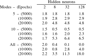
An example of this parametric sweep is shown in table 1. Here, the relative error (displayed in per cent) has been tabulated as a function of hidden neurons, number of POD modes, and number of training epochs. In all cases shown here, a single hidden layer was used, with gradient descent and no momentum. The neural nets were trained on the first 750 sets of synchronous PIV–microphone data (taken from the
 $St_{DF}=0.25$
excited jet), and validated on the last 750 sets. The error in the validation was computed as the sum-of-squares error between the known velocity fluctuation vectors and those produced by the neural net.
Overfitting the training data is a common concern with neural networks, due to the large number of free parameters that exist between the input, hidden, and output neurons. This problem is evident here, where for the greatest number of POD modes and hidden neurons (and hence the greatest number of free parameters) and greatest number of training epochs, the error in the estimations was 18 % greater than that of the most optimum configuration. It’s not shown here, but the sum-of-squares error for the training dataset was the lowest for this configuration. However, the error in the validation dataset is relatively insensitive to network parameters over a broad range of conditions. In general, using a greater number of hidden neurons and POD modes, while using fewer training epochs is found to produce the optimal accuracy in the estimations. Using even fewer than 5000 epochs might be tempting, although this risks producing a poorly converged solution if the initial weight vectors (which are set randomly) are located on a plateau of the cost function.
Though not shown here for brevity, the effects of varying other parameters was also investigated. Another common technique to prevent overfitting is the use of regularization,
 $L_{1}$
being the preferred method. Adding a regularization parameter was found to have an effect similar to limiting the number of training epochs, and in many cases produced more consistent results. However, the best result from the regularization cases were still roughly 0.5 % worse than the optimal configuration shown here, so it was not used in this work. Additionally, changing the learning-rate parameter or using momentum was investigated, but did not provide better results. Finally, a well-known issue with the gradient descent optimization method is that it has a tendency to get trapped in local minima and fails to converge to the global minimum. Therefore, sample results were also calculated using adaptive particle swarm optimization, although the results were found to not differ substantially from those produced by the backpropagation algorithm.
Axial velocity field for a snapshot from the (a) original validation dataset and (b) estimated from the optimal neural network configuration.

A sample comparison of the raw and estimated velocity fields from the validation data subset is shown in figure 20. In figure 20(a) the axial velocity from a PIV snapshot in the validation subset is plotted. In figure 20(b) the axial velocity field estimated by a neural network tuned using the training data subset is plotted. The inputs to the neural network are the microphone pressure traces acquired simultaneously to the PIV snapshot shown in figure 20(a). Admittedly, the neural network’s estimation is imperfect, losing much of the small-wavelength, incoherent structures inherent to the turbulent mixing layer (along with experimental noise, such as vectors dropped due to poor correlations and which were replaced by zero vectors). Overall, the large-scale features of the coherent structures have been well captured; accelerations and decelerations in the jet core, associated with the passage of large-scale structures, are observed in both figures at matching radial and axial positions; slight asymmetries in the large-scale structures are also captured in some places. The high-velocity region centred around
 $x/D\simeq 4.5$
is a good example of this; the leading half of the structure (or likely, two structures that are merging) is slightly skewed towards the negative radial plane and this is replicated by the neural network estimation. A significant error in the estimation is observed downstream of the end of the potential core, where the PIV snapshot exhibits a large-scale acceleration centred around
 $x/D\simeq 10.5$
whereas this structure is completely absent in the estimation velocity field. This degradation in accuracy is likely the result of the ring vortices collapsing as they pass through the end of the potential core, leading to highly three-dimensional structures which cannot be well-correlated between microphones and laser sheets that lie on different azimuthal planes.