A. Formulation

We begin with a two-dimensional crystal consisting of atomic cores (not necessarily carbon) and conduction electrons. This contains the implicit assumption that the problem is separable into planar (x, y) variables and a transverse variable z that is omitted. Consider the model Hamiltonian,

(2.1) $${H_n} = \left\{ {\sum\limits_{j = 1}^n {\left[ { - {{{\hbar ^2}} \over {2m}}\nabla _j^2 + \sum\limits_J {{v_{{\rm{core}}}}\left( {\left| {{{\vec R}_J} - {{\vec r}_j}} \right|} \right)} } \right]} + {1 \over 2}\sum\limits_{j,j'}^n {v\left( {\left| {{{\vec r}_j} - {{\vec r}_{j'}}} \right|} \right)} } \right\}\quad ,$$

where j = 1, 2, …, n are electrons whose two-dimensional position and spin variables are combined in ${\vec r_j}$ , J labels atomic cores, v _core is the electron-core interaction, and v, the effective electron–electron interaction, is taken to be pairwise and cylindrically symmetrical.

Now, the core terms $\hbox( {\sum\limits_J {} } \hbox)$ constitute the periodic potential of the crystal. If the conduction electrons are approximately like noninteracting electrons at the bottom of the first conduction band of the crystal, then the periodic potential may be replaced by an effective band mass m _b in place of the free-electron mass m. We express this in terms of a dimensionless parameter µ,

(2.2) $${m_{\rm{b}}} = \mu \cdot m\quad .$$

We can now rewrite the Hamiltonian H _n in Bohr–Hartree atomic units,

(2.3) $${H_n} = \sum\limits_{j = 1}^n {\left[ { - {1 \over {2\mu }}\nabla _j^2 + {1 \over 2}\sum\limits_{j' = 1}^n {v\left( {{{\vec r}_j} - {{\vec r}_{j'}}} \right)} } \right]} \quad .$$

Units of length are now Bohr (a ₀), and units of energy are Hartree (Hy), where

(2.4) $${a_0} = {{4\pi {\varepsilon _0} \cdot {\hbar ^2}} \over {m{e^2}}} = 0.529\;{\rm{A}},\quad 1\;{\rm{Hy}} = {{{\hbar ^2}} \over {ma_0^2}} = 27.2\;{\rm{eV}}\quad .$$

The pairwise interaction is now expressed in Hy units. Note especially that in Eq. (2.3), the periodic potential, if any, will arise from $v\left( {\vec r} \right)$ , expressing the CDW, not from the periodicity of the atomic ordering in the crystal, which is expressed by the band mass parameter µ.

The physics of our model system should include the phonons of the crystal and their energy, and the electron–phonon interaction and its energy. We assume that the electron–phonon interaction produces a modification of the electron–electron interaction and phonon–phonon interaction with the resultant effective electron and phonon dynamical variables becoming separable, the electron–phonon interaction having been subsumed into the new electronic and phononic parts of the system Hamiltonian. We can then analyze the electronic part, as in Eq. (2.1), and treat the phonon part as a fixed, constant part of the total energy. In this case, the effective pairwise electron–electron interaction, $v\left( {\vec r} \right)$ in Eq. (2.1), contains a phonon-mediated contribution, in addition to the Coulomb repulsion. While these postulates are not likely to be justifiable in general, the resultant model may mimic specific properties of some systems.

B. The total energy

It is our purpose, both in the system’s model and in the computation of its properties, especially its total energy, to use as simplified an approach as possible. The total energy E _n from Eq. (2.3) is

(2.5) $${E_n} = \left\langle {{\Psi _n}\left| {{H_n}} \right|{\Psi _n}} \right\rangle \quad ,$$

where Ψ _n is the ground state many-electron wave function and E _n is its eigenvalue. For simplicity, consider the Hartree approximation, where

(2.6) $${\Psi _n}\left( {{{\vec r}_1},{{\vec r}_2}, \ldots ,{{\vec r}_n}} \right) = \prod\limits_{j = 1}^n {{\psi _j}\left( {{{\vec r}_j}} \right)} \quad ,$$

where ${\psi _j}\left( {{{\vec r}_j}} \right)$ is a set of n orthonormal single particle functions. If such a set has to minimize E _n , it must satisfy the Hartree equation,

(2.7) $$h\left( {\vec r} \right) \cdot {\psi _j}\left( {\vec r} \right) = {\varepsilon _j} \cdot {\psi _j}\left( {\vec r} \right)\quad ,$$

where the Hartree operator h is

(2.8) $$h\left( {\vec r} \right) = - {1 \over {2\mu }}{\nabla ^2} + \sum\limits_{j' = 1}^n {\left\langle {j'\left| v \right|j'} \right\rangle } \quad ,$$

(2.9) $$\left\langle {j'\left| v \right|j'} \right\rangle = \int {{{\rm{d}}^2}r' \cdot \psi _{j'}^ * } \left( {\vec r'} \right) \cdot v\left( {\vec r - \vec r'} \right) \cdot {\psi _{j'}}\left( {\vec r'} \right)\quad .$$

From Eqs. (2.7) and (2.8), if we sum over j from j = 1 to j = n and compare the result that comes from Eqs. (2.3) and (2.6), we arrive at the well-known conclusion that the two-particle contribution to the energy is double counted in the Hartree equation. We shall therefore evaluate the total energy E _n by summing over the n single-particle Hartree energies ε _j and then subtracting half of the potential energies that are included in that sum,

(2.10) $${E_n} = \sum\limits_{j = 1}^n {{\varepsilon _j} - {1 \over 2}\sum\limits_{j,j' = 1}^n {\left\langle {j,j'\left| v \right|j,j'} \right\rangle } } \quad ,$$

see Eqs. (2.5)–(2.9).

C. Electron density

For our study of CDW, it is useful to include the electron density operator ${\rho _{{\rm{op}}}}\left( {\vec r} \right)$ in the formulation. Consider,

(2.11) $${\rho _{{\rm{op}}}}\left( {\vec r} \right) = \sum\limits_{j = 1}^n {\delta \left( {\vec r - {{\vec r}_j}} \right)} \quad .$$

We now introduce Ω as the Born-von Karman area of a system consisting of n electrons in N primitive unit cells of the Bravais lattice, subject to periodic boundary conditions. In terms of its Fourier analysis, ${\rho _{{\rm{op}}}}\left( {\vec r} \right)$ is

(2.12) $${\rho _{{\rm{op}}}}\left( {\vec r} \right) = \sum\limits_{\vec k} {{\rho _{\vec k}} \cdot \exp \left( {i\vec k \cdot \vec r} \right)} \quad ,$$

(2.13) $${\rho _{\vec k}} = {1 \over \Omega }\int {{{\rm{d}}^2}r' \cdot {\rho _{{\rm{op}}}}\left( {\vec r'} \right) \cdot \exp \left( { - i\vec k \cdot r'} \right)} = {1 \over \Omega }\sum\limits_{j = 1}^n {\exp \left( { - i\vec k \cdot {{\vec r}_j}} \right)} \quad .$$

D. The self-consistent field

The two-particle term in the Hartree Eq. (2.9) is called the self-consistent field, denoted scf. It is related to the electron density as follows. Consider the Fourier transform relation,

(2.14) $$v\left( {\vec r} \right) = \sum\limits_{\vec k} {{v_{\vec k}} \cdot \exp \left( {i\vec k \cdot \vec r} \right)} \quad ,$$

(2.15) $${v_{\vec k}} = {1 \over \Omega }\int {{{\rm{d}}^2}r' \cdot v\left( {\vec r'} \right) \cdot \exp \left( { - i\vec k \cdot \vec r} \right)} \quad .$$

Then in the scf, we have

(2.16) $${ \sum\limits_{j' = 1}^n {\left\langle {j'\left| {v\left( {\vec r - \vec r'} \right)} \right|j'} \right\rangle } = \sum\limits_{\vec k} {{v_{\vec k}} \cdot \exp \left( {i\vec k \cdot \vec r} \right)} \cdot \sum\limits_{j' = 1}^n {\int {{{\rm{d}}^2}r'{{\left| {{\psi _{j'}}\left( {\vec r'} \right)} \right|}^2} \cdot \exp \left( { - i\vec k \cdot \vec r'} \right)\quad .} } \cr}$$

Now in Eq. (2.16), the sum over j′ on the right-hand side is the expectation value of $\left( {\Omega \cdot {\rho _{\vec k}}} \right)$ , Eq. (2.13), in the many-body state Ψ, Eq. (2.6). Thus, if we denote

(2.17) $$\left\langle {\Psi \left| {{\rho _{\vec k}}} \right|\Psi } \right\rangle = \left\langle {{\rho _{\vec k}}} \right\rangle \quad ,$$

then the Hartree Eqs. (2.7) and (2.8) become

(2.18) $$\left[ { - {1 \over {2\mu }}{\nabla ^2} + \Omega \cdot \sum\limits_{\vec k} {{v_{\vec k}} \cdot \left\langle {{\rho _{\vec k}}} \right\rangle \cdot \exp \left( { - i\vec k \cdot \vec r} \right)} } \right]{\psi _j}\left( {\vec r} \right) = {\varepsilon _j} \cdot {\psi _j}\left( {\vec r} \right)\quad .$$

E. Graphene structure in a CDW

Graphene consists of a planar array of carbon atoms in a space filling set of open hexagons—see Fig. 1(a). The crystal basis consists of two nearest neighbor atoms at sites (1) and (2), for example, in Fig. 1(a), separated by the displacement vector ${\vec a_0}$ of magnitude a ₀ [not to be confused with the Bohr radius a ₀ in Eq. (2.4)]. The primitive translation vectors of the crystal lattice are ${\vec a_1}$ and ${\vec a_2}$ , where

(2.19) $${\vec a_1} = {a \over 2}\left( {\sqrt 3 \hat i + \hat j} \right),\;{\vec a_2} = {a \over 2}\left( {\sqrt 3 \hat i - \hat j} \right)$$

and where

(2.20) $$a = \left| {{{\vec a}_1}} \right| = \left| {{{\vec a}_2}} \right| = \sqrt 3 \cdot {a_0}\quad ,$$

and $\hat i$ and $\hat j$ are unit vectors in the x and y directions. The reciprocal lattice basis vectors are

(2.21) $${\vec b_1} = {{2\pi } \over a}\left( {{1 \over {\sqrt 3 }}\hat i + \hat j} \right),\;{\vec b_2} = {{2\pi } \over a}\left( {{1 \over {\sqrt 3 }}\hat i - \hat j} \right)\quad ,$$

with the defining property

(2.22) $$\left( {{{\vec b}_i} \cdot {{\vec a}_j}} \right) = 2\pi {\delta _{ij}},\;b = \left| {{{\vec b}_j}} \right| = {{4\pi } \over {3{a_0}}}\quad .$$

FIG. 1.

(a) Hexagonal unit of graphene crystal, with basis sites (1) and (2) and separation ${\vec a_0}$ , primitive translation vectors ${\vec a_1}$ and ${\vec a_2}$ , and x–y coordinate axes. (b) Hexagonal first Brillouin zone in the reciprocal lattice of the graphene crystal, with primitive translation vectors ${\vec b_1}$ and ${\vec b_2}$ , and k _x − k _y coordinates.

The reciprocal lattice hexagonal unit is shown in Fig. 1(b). Notice the (π/6) rotation between the hexagons in Figs. 1(a) and 1(b).

We now return to our Hartree Eq. (2.18). For a CDW, we require that the scf consists of a wave pattern that has the geometrical shape of the atomic core pattern of graphene, Fig. 1(a). We must keep in mind that our system, Eq. (2.18), contains no atomic cores. They have been subsumed into the effective electron mass parameter µ, Eq. (2.2). It will now be the phonon mediated part of ${v_{\vec k}}$ in Eq. (2.18) that enables the system to have an scf in the form of a CDW. This may occur if the scf is dominated by $\vec k$ values that reflect the electronic structure of graphene. Thus consider

(2.23) $$\vec k = \pm {\vec K_1},\; \pm {\vec K_2},\; \pm {\vec K_3}\quad ,$$

where

(2.24) $${\vec K_1} = {\vec b_1},\;{\vec K_2} = {\vec b_2},\;{\vec K_3} = \left( {{{\vec K}_1} + {{\vec K}_2}} \right) = \left( {{{\vec b}_1} + {{\vec b}_2}} \right)\quad .$$

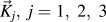
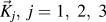
Vectors ${\vec K_1}$ and ${\vec K_2}$ ensure that our scf has the correct translational properties, and ${\vec K_3}$ is required to reflect the two-atom basis of graphene. All three vectors ${\vec K_j},\;j = 1,\;2,\;3$ have the same magnitude K = b, where K determines the scale a ₀ of the wave pattern, see Eq. (2.22).

The six wave vectors in Eq. (2.23) taken together give three cosines. Consider,

(2.25) $$F\left( {\vec r} \right) = \sum\limits_{j = 1}^3 {\cos \left( {{{\vec K}_j} \cdot \vec r} \right)} \quad .$$

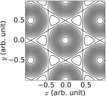
This wave pattern is shown as a contour map in Fig. 2. The large dark areas are centered on triangular mesh sites at wave pattern maxima. They tend toward hexagonal shape, representing each one’s relationship with six nearest neighbor minima. The latter is shown as light area, tending toward triangular shape, representing each one’s relationship with three nearest neighbor maxima. The minima correspond to atomic sites in graphene. The wave pattern therefore exactly reflects the potential seen by valence electrons in graphene.

FIG. 2.

Wave pattern, Eq. (2.25), of our two-dimensional CDW model with the graphene structure.

Now for our scf in Eq. (2.18) to behave like $F\left( {\vec r} \right)$ in Eq. (2.25), we require the coefficients

(2.26) $$\left( {{v_{\vec k}}.\left\langle {{\rho _{\vec k}}} \right\rangle } \right);\;\vec k = \pm {\vec K_j},\;j = 1,\;2,\;3$$

all to be equal. Since $v\left( {\vec r} \right)$ and $\rho \left( {\vec r} \right)$ are real, we see that

(2.27) $${v_{\vec k}} = {v_{ - \vec k}}\;{\rm{and}}\;{\rho _{\vec k}} = {\rho _{ - \vec k}}\quad .$$

Furthermore, in Fig. 1(b), we see that vectors ${\vec K_j},\;j = 1,\;2,\;3$ are all equivalent in relation to the reciprocal lattice of the graphene structure, as well as in relation to each other. It follows that

(2.28) $$\left( {{v_{{{\vec K}_j}}} \cdot {\rho _{{{\vec K}_j}}}} \right) = \left( {{v_K}\left\langle {{\rho _K}} \right\rangle } \right),\quad j = 1,\;2,\;3\quad .$$

The quantity v _K is the second fundamental parameter of our model, the others being the effective band mass µ, Eq. (2.2) and the CDW number K. This completes our model for a CDW having the graphene electronic structure, determined in terms of the Hartree Eq. (2.18), now in the form,

(2.29) $$\left[ { - {1 \over {2\mu }}{\nabla ^2} + 2{\Omega ^2} \cdot {v_K} \cdot \left\langle {{\rho _K}} \right\rangle \cdot \sum\limits_{j' = 1}^3 {\cos \left( {{{\vec K}_{j'}} \cdot \vec r} \right)} } \right] \cdot {\psi _j}\left( {\vec r} \right) = {\varepsilon _j} \cdot {\psi _j}\left( {\vec r} \right)\quad .$$

A. Tight-binding approximation

We now undertake the solution of Eq. (2.29). The discovery of the electronic structure of graphene dates from Wallace’s 1947 paper, ^{Reference Novoselov, Geim, Morozov, Jiang, Zhang, Dubonos, Grigorieva and Firsov2} before the era of electronic computation. Using only analytical methods applied in very simple approximations, Wallace was able to get the qualitative features of graphene correctly. Since that approach was successful, and fits with our objective of keeping our analysis as simple as possible, we shall follow Wallace’s work closely. To this end, we introduce the tight-binding approximation. It is briefly described by Wallace and in more detail by Ashcroft and Mermin. ^{Reference Ashcroft and Mermin6}

We begin with Bloch functions of Wannier type, see Wallace’s Eq. (2.2). Because of the diatomic nature of our crystal basis, we view the crystal lattice as a superposition of two sublattices, A and B. Then the normalized Hartree eigenfunctions in Eq. (2.29) are

(3.1) $${\psi _{\vec k}}\left( {\vec r} \right) = {1 \over {\sqrt n }}\left\{ {{\varphi _{1,\vec k}}\left( {\vec r} \right) \pm {\varphi _{2,\vec k}}\left( {\vec r} \right)} \right\}\quad ,$$

where ± refers to states outside/inside BZI, and where

(3.2) $${\varphi _{1,\vec k}} = \sum\limits_A {\exp \left( {i\vec k \cdot {{\vec R}_A}} \right) \cdot {\rm X}\left( {\vec r - {{\vec R}_{\rm{A}}}} \right)\quad ,}$$

(3.3) $${\varphi _{2,\vec k}} = \sum\limits_B {\exp \left( {i\vec k \cdot {{\vec R}_B}} \right) \cdot {\rm X}\left( {\vec r - {{\vec R}_B}} \right)\quad ,}$$

with ${\rm X}\left( {\vec r} \right)$ a normalized ground state atomic-like orbital. Note that we have now labeled ψ _j by $\vec k$ values, where $\vec k$ ranges over the n occupied Hartree eigenstates constituting the first Brillouin zone, BZI, similarly for ε _j to become ${\varepsilon _{\vec k}}$ . Now following Wallace, for the single particle energy, here ${\varepsilon _{\vec k}}$ and in Wallace E, we have

(3.4) $${\varepsilon _{\vec k}} = \left\{ {{{h'}_{11}}\left( {\vec k} \right) \pm \left| {{{h'}_{12}}\left( {\vec k} \right)} \right|} \right\}\quad .$$

In Eq. (3.4),

(3.5) $${h'_{11}}\left( {\vec k} \right) = \int {{{\rm{d}}^2}r \cdot \varphi _{1,\vec k}^ * } \left( {\vec r} \right) \cdot h\left( {\vec r} \right) \cdot {\varphi _{1,\vec k}}\left( {\vec r} \right)\quad ,$$

(3.6) $${h'_{12}}\left( {\vec k} \right) = \int {{{\rm{d}}^2}r \cdot \varphi _{1,\vec k}^ * } \left( {\vec r} \right) \cdot h\left( {\vec r} \right) \cdot {\varphi _{2,\vec k}}\left( {\vec r} \right).$$

We now implement the tight-binding approximation by neglecting all but nearest-neighbor overlap integrals in sublattice A (or B) for the atomic-like orbitals ${\rm X}\left( {\vec r} \right)$ in ${h'_{11}}$ , Eq. (3.5), and further, neglecting all but nearest-neighbor integrals between sublattices A and B in ${h'_{12}}$ , Eq. (3.6).

Still following Wallace, we introduce the periodic potential V of the system. In the present case, this is the scf in Eq. (2.29),

(3.7) $$V\left( {\vec r} \right) = 2{\Omega ^2} \cdot {v_K} \cdot \left\langle {{\rho _K}} \right\rangle \cdot \sum\limits_{j = 1}^3 {\cos \left( {{{\vec K}_j} \cdot \vec r} \right)\quad .}$$

We also introduce the potential $U\left( {\vec r} \right)$ for an isolated atomic-like orbital, determined from the minima of $V\left( {\vec r} \right)$ . The precise analytical form of $U\left( {\vec r} \right)$ will be given in Sec. III.B. It is the combination (U–V) that is central to the tight-binding approximation. Then from Wallace, and verifying his results, we obtain

(3.8) $${h'_{11}} = {\varepsilon _0} - 2{\gamma '_0}\left[ {2\cos \left( {{{\sqrt 3 } \over 2}a{k_x}} \right)\cos \left( {{1 \over 2}a{k_y}} \right) + \cos \left( {a{k_y}} \right)} \right]\quad ,$$

(3.9) $$\left| {{{h'}_{12}}} \right| = {\gamma _0}{\left[ {1 + 4{{\cos }^2}\left( {{1 \over 2}a{k_y}} \right) + 4\cos \left( {{1 \over 2}a{k_y}} \right)\cos \left( {{{\sqrt 3 } \over 2}a{k_x}} \right)} \right]^{1/2}}\quad .$$

In Eq. (3.8),

(3.10) $${\varepsilon _0} = \int {{{\rm{d}}^2}r \cdot {{\rm X}^*}\left( {\vec r} \right) \cdot h\left( {\vec r} \right) \cdot {\rm X}\left( {\vec r} \right)\quad ,}$$

(3.11) $${\gamma '_0} = \int {{{\rm{d}}^2}r \cdot {{\rm X}^ * }\left( {\vec r} \right) \cdot h\left( {\vec r} \right) \cdot {\rm X}\left( {\vec r - {{\vec R}_A}} \right)} \quad ,$$

where ${\vec R_A}$ is any nearest-neighbor displacement of an atomic-like position from the origin in sublattice A. In Eq. (3.9),

(3.12) $${\gamma _0} = \int {{{\rm{d}}^2}r \cdot {{\rm X}^ * }\left( {\vec r} \right) \cdot h\left( {\vec r} \right) \cdot {\rm X}\left( {\vec r - {{\vec R}_B}} \right)\quad ,}$$

where ${\vec R_B}$ has the same meaning in sublattice B. From Fig. 1(a), we see that

(3.13) $${\vec R_A} = {\vec a_1},\;{\vec R_B} = {\vec a_0}\quad .$$

From the tight-binding approximation, we now have

(3.14) $${\gamma '_0} = \int {{{\rm{d}}^2}r \cdot {{\rm X}^ * }\left( {\vec r} \right) \cdot \left[ {U\left( {\vec r} \right) - V\left( {\vec r} \right)} \right] \cdot {\rm X}\left( {\vec r - {{\vec a}_1}} \right)\quad ,}$$

(3.15) $${\gamma _0} = \int {{{\rm{d}}^2}r \cdot {{\rm X}^ * }\left( {\vec r} \right) \cdot \left[ {U\left( {\vec r} \right) - V\left( {\vec r} \right)} \right] \cdot {\rm X}\left( {\vec r - {{\vec a}_0}} \right)\quad .}$$

Note that ε₀ is the energy of an electron in the atomic-like potential $U\left( {\vec r} \right)$ . Also note that our definitions of U and V are vice versa to the definitions used by Ashcroft and Mermin. ^{Reference Ashcroft and Mermin6} Eq. (3.4), along with all the other formulae of this subsection, constitutes the tight-binding solution of our Hartree equation. However, we have yet to specify the atomic-like orbitals ${\rm X}\left( {\vec r} \right)$ in Eqs. (3.2) and (3.3).

B. Atomic-like orbitals

For our two-dimensional waveform $V\left( {\vec r} \right)$ , consisting of three harmonic waves, Eq. (3.7), we approximate $V\left( {\vec r} \right)$ in the region near one of its minima by the lowest order fit, namely, a cylindrically symmetrical quadratic form, $U\left( {\vec r} \right)$ ,

(3.16) $$U\left( {\vec r} \right) = \left( { - A + {1 \over 2}B \cdot {r^2}} \right)\quad .$$

This potential will define our atomic-like orbitals ${\rm X}\left( {\vec r} \right)$ . In Eq. (3.16), we have introduced a negative sign based on the assumption that A is positive because the minima of $V\left( {\vec r} \right)$ come from the minima of three cosines, all of which are negative at their minima. An electron in such a potential satisfies a two-dimensional cylindrical Schrödinger equation,

(3.17) $$\left[ { - {1 \over {2\mu }} \cdot {\nabla ^2} + \left( { - A + {1 \over 2}B{r^2}} \right)} \right] \cdot {\rm X}\left( {\vec r} \right) = {\varepsilon '_0} \cdot {\rm X}\left( {\vec r} \right)\quad .$$

Consider a trial form for ${\rm X}\left( {\vec r} \right)$ ,

(3.18) $${\rm X}\left( r \right) = \sqrt {{2 \over {\rm{\pi }}}} \cdot \alpha \cdot \exp \left( { - {\alpha ^2}{r^2}} \right)\quad ,$$

i.e., a normalized harmonic oscillator ground state wave function. If it is to be an eigenfunction in Eq. (3.17), we must have

(3.19) $$B = {{4{\alpha ^4}} \over \mu }$$

and

(3.20) $${\varepsilon '_0} = \left( {{{2{\alpha ^2}} \over \mu } - A} \right)\quad .$$

Now in Eq. (3.16), (−A) is the minimum value of our scf potential Eq. (3.7), and B is its curvature. First consider (−A),

(3.21) $$\left( { - A} \right) = 2\Omega \cdot {v_K} \cdot \left\langle {{\rho _K}} \right\rangle \cdot {\left[ {\sum\limits_{j = 1}^3 {\cos \left( {{{\vec K}_j} \cdot \vec r} \right)} } \right]_{\vec r = {{\vec r}_1}}}\quad ,$$

where ${\vec r_1}$ is a minimum of $V\left( {\vec r} \right)$ . For example, atomic-like site (3) in Fig. 1(a) has position,

(3.22) $${\vec r_1} = {a \over {2\sqrt 3 }} \cdot \left( {\hat i + \sqrt 3 \hat j} \right)$$

so

(3.23) $$A = 3 \cdot \Omega \cdot {v_K}\left\langle {{\rho _K}\left( \alpha \right)} \right\rangle \quad .$$

It follows from Eqs. (3.20) and (3.23) that the atomic-like ground state energy is

(3.24) $${\varepsilon '_0} = \left[ {{{2{\alpha ^2}} \over \mu } - 3\Omega \cdot {v_K}\left\langle {{\rho _K}\left( \alpha \right)} \right\rangle } \right]\quad .$$

Now regarding B, the requirement that Eq. (3.17) should be an eigenvalue equation gives us Eq. (3.19). However, we also require B to make U(r), Eq. (3.16), fit the curvature of the potential $V\left( {\vec r} \right)$ at its minimum. The second order terms from the expansion of V(r) about $\vec r = {\vec r_1}$ are

(3.25) $${ {1 \over 2}{\sum\limits_{\alpha ,\beta \simeq 1}^2 {\left[ {{{{\partial ^2}} \over {\partial {\chi _\alpha } \cdot \partial {\chi _\beta }}}\left[ {2\Omega \cdot {v_K} \cdot \left\langle {{\rho _K}} \right\rangle \cdot \sum\limits_{j = 1}^3 {\cos \left( {{{\vec K}_j} \cdot \vec r} \right)} } \right] \cdot {\chi _\alpha }{\chi _\beta }} \right]} _{\vec r = {{\vec r}_1}}} = \Omega \cdot {v_K} \cdot \left\langle {{\rho _K}} \right\rangle \cdot {\left( {{{2\pi } \over a}} \right)^2} \cdot {r^2}\quad . \cr}$$

In Eq. (3.25), χ₁ = x, χ₂ = y, r ² = (x ² + y ²). Thus combining Eqs. (3.19) and (3.25), we have

(3.26) $$B = {{4{\alpha ^4}} \over \mu } = 2\Omega \cdot {v_K} \cdot \left\langle {{\rho _K}} \right\rangle \cdot {\left( {{{2\pi } \over a}} \right)^2}\quad .$$

This is a powerful constraint upon the solution of the Hartree equation, and as we shall see, it plays a central role in the analysis of the model system.

A. Occupied $\vec k$ -space region in the ground state

To examine the scf more fully, we need explicit knowledge of 〈ρ _K 〉. From Eqs. (2.13) and (2.6),

(4.1) $$\left\langle {{\rho _K}} \right\rangle = {1 \over \Omega } \cdot \sum\limits_{j = 1}^n {\int {{d^2}r\psi _j^ * \left( {\vec r} \right) \cdot \exp \left( { - i\vec K \cdot \vec r} \right) \cdot {\psi _j}\left( {\vec r} \right)\quad .} }$$

In Sec. III.A, we have cast the Hartree eigenstates in terms of $\vec k$ values, Eq. (3.1) and later. Thus, consider the first Brillouin zone, denoted BZI: It consists of $\vec k$ -space values within the mutual limits,

(4.2) $$\vec k = \pm {{{{\vec b}_i}} \over 2},\;i = 1,\;2;\;{{{{\vec b}_3}} \over 2} = {{\left( {{{\vec b}_1} + {{\vec b}_2}} \right)} \over 2}$$

or

(4.3) $$\vec k = \pm {{{{\vec K}_i}} \over 2},\;i = 1,\;2,\;3\quad ,$$

see Eqs. (2.23) and (2.24). This area, A _BZI, is therefore

(4.4) $${A_{{\rm{BZI}}}} = {{\sqrt 3 } \over 2} \cdot {b^2}\quad .$$

The density $D\left( {\vec k} \right)$ of $\vec k$ -space points is

(4.5) $$D\left( {\vec k} \right) = {\Omega \over {{{\left( {2\pi } \right)}^2}}}\quad ,$$

where Ω is the area of the Born-von Karman region containing n electrons in N primitive unit cells of the Bravais lattice, each containing two electrons,

(4.6) $$N = {n \over 2}\quad .$$

Thus from Eqs. (4.4) and (4.5), the number of one-electron states in BZI including spin is

(4.7) $$2 \cdot {A_{{\rm{BZI}}}} \cdot D\left( {\vec k} \right) = 2 \cdot \left( {{{\sqrt 3 } \over 2} \cdot {b^2}} \right) \cdot \left( {{\Omega \over {{{\left( {2\pi } \right)}^2}}}} \right)\quad .$$

Now Ω is

(4.8) $$\Omega = N \cdot \left| {{{\vec a}_1} \times {{\vec a}_2}} \right| = n{a^2} \cdot {{\sqrt 3 } \over 4}\quad ,$$

from Eqs. (4.6) and (2.19). We obtain the value of b from Eq. (2.21), giving for Eq. (4.7),

(4.9) $$2 \cdot {A_{{\rm{BZI}}}} \cdot D\left( {\vec k} \right) = n\quad .$$

This verifies that the number of electrons in our CDW exactly fills BZI. Wallace ^{Reference Wallace1} has shown that all the Hartree eigenstates in BZI have lower energy than those outside.

B. The role of average electronic density in CDW

The average electronic density in $\vec r$ -space, ρ₀, is

(4.10) $${\rho _0} = {n \over \Omega }\quad .$$

From Eq. (4.8), and the relationship between a and K, Eqs. (2.19) and (2.21), we find

(4.11) $${\rho _0} = \sqrt 3 {\left( {{K \over {2\pi }}} \right)^2}$$

or

(4.12) $$K = \left( {2\pi } \right) \cdot {\left( {{{{\rho _0}} \over {\sqrt 3 }}} \right)^{1/2}}\quad .$$

In other words, Eq. (4.11) tells us that if a CDW is required with a given value of K, then the average density must have the value specified there. On the other hand, if our system has a given density ρ₀, the only K-value which can form in a CDW is given by Eq. (4.12).

C. Evaluation of 〈ρ _K 〉

We must now evaluate 〈ρ _K 〉, Eq. (4.1). There, we convert the sum over j to an integral over $\vec k$ -space in BZI, (×2) for spin,

(4.13) $$\sum\limits_{j = 1}^n { \to 2 \cdot \int_{{\rm{BZI}}} {{{\rm{d}}^2}k \cdot D\left( {\vec k} \right)\quad .} }$$

In Eq. (4.1), expressed in terms of $\vec k$ , ${\psi _{\vec k}}\left( {\vec r} \right)$ is given by Eqs. (3.1)–(3.3), and (3.18), with the sums over ${\vec R_A}$ and ${\vec R_B}$ limited according to our application of the tight-binding approximation. The resultant evaluation has been determined analytically by using MATLAB and MAPLE independently, with the result,

(4.14) $$\left\langle {{\rho _K}} \right\rangle = {1 \over {{a^2}}} \cdot f\left( w \right)\quad ,$$

where

(4.15) $$w = {\left( {\alpha a} \right)^2}$$

and

(4.16) $$f\left( w \right) = \exp \left( { - {{2{\pi ^2}} \over {3w}}} \right) \cdot \left[ {{1 \over {2{\pi ^2}}} \cdot \left( {6\sqrt 3 + 4\pi } \right) \cdot \exp \left( { - {w \over 6}} \right) - {2 \over {\sqrt 3 }}} \right]\quad .$$

D. Self-consistency

We now evaluate the scf condition expressed by Eq. (3.26), using the notation w, Eq. (4.15), the expression for 〈ρ _K 〉, Eqs. (4.14)–(4.16), and

(4.17) $${v_K} = {1 \over \Omega }\int {{{\rm{d}}^2}r \cdot v\left( r \right) \cdot \exp \left( { - i\vec K \cdot \vec r} \right)\quad .}$$

The result is

(4.18) $${w^2} = \left( {\mu .{{\tilde v}_K}} \right) \cdot f\left( w \right)\quad ,$$

where

(4.19) $${\tilde v_K} = 2{\pi ^2} \cdot \int {{{\rm{d}}^2}r \cdot v\left( r \right) \cdot {e^{ - i\vec K \cdot \vec r}} = 2{\pi ^2} \cdot \Omega \cdot {v_K}} \quad .$$

Equation (4.18) is the self-consistency condition required for a solution to the Hartree equation within the context of the tight-binding approximation as applied to a CDW. Only values of w that satisfy Eq. (4.18) may be used in calculating properties of the CDW system, such as the total energy.

From its definition, Eq. (4.15), w must be positive. From Eq. (4.18), several possibilities arise. Basically, it is required that

(4.20) $$\left( {\mu \cdot {{\tilde v}_K}} \right) \cdot f\left( w \right) > 0\quad .$$

We shall exemplify the possible solutions by considering here only the case,

(4.21) $$\mu > 0\quad .$$

We remark that the case μ < 0 means that the electron gas consists of hole-like, rather than electron-like, quasiparticles.

Now from Eqs. (4.20) and (4.21), two possibilities remain as follows:

(4.22) $${\rm{Case}}\;\left( {\rm{i}} \right):\;{\tilde v_K} > 0\;{\rm{and}}\;f\left( w \right) > 0\quad ,$$

(4.23) $${\rm{Case}}\;\left( {{\rm{ii}}} \right):\;{\tilde v_K} \lt 0\;{\rm{and}}\;f\left( w \right) \lt 0\quad .$$

Consider Case (i). From Eq. (4.16), we find that f(w) is positive only for

(4.24) $$0 \le w \le 0.0435\quad .$$

For w = 0.0435, ∝ ≈ (0.2/a) ≈ 1/(5a). Now ∝ is a measure of the range R of the Gaussian atomic-like orbital, namely, the distance at which the orbital’s amplitude is e ⁻¹ ≈ 0.37 times its maximum value. Thus we find that for f(w) > 0,

(4.25) $$w = {\left( {\alpha a} \right)^2} = {\left( {{a \mathord{\left/ {\vphantom {a R}} \right. \kern-\nulldelimiterspace} R}} \right)^2} \lt 0.0435\quad ,$$

whence

(4.26) $$R > 8.3{a_0}\quad ,$$

where a ₀ is the nearest-neighbor distance in the graphene structure. However, implicit in the tight-binding approximation is the assumption that the atomic-like orbitals are well-localized within a range R ≲ a ₀. Thus the solution with f(w) > 0 is inconsistent with the present model. We conclude that Case (i) is unphysical. At this point, we therefore conclude, perhaps not surprisingly, that with μ > 0, ${\tilde v_K}$ and therefore v _K must be negative, i.e., attractive. It means that, at wave number K, the phonon-mediated part of the pairwise interaction must be attractive and must overwhelm the corresponding component of the Coulomb repulsion so that the total interaction is also attractive.

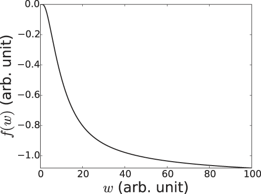
Now consider Case (ii), with ${\tilde v_K} \lt 0$ and f(w) < 0. The latter condition is found to be valid for w > 0.0435. Figure 3 shows the plot of f(w) versus w, with a horizontal asymptote at |f(w)| = 1.1547. We now express the scf condition in terms of w as a function of $x = \left( {\mu \cdot \left| {{{\tilde v}_K}} \right|} \right)$ , with μ > 0,

(4.27) $${{{w^2}} \over {\left| {f(w)} \right|}} = x\quad .$$

FIG. 3.

f(w), Eq. (4.16), plotted versus w.

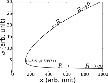
This is plotted in Fig. 4, where the coordinates for a minimum value of x are given, showing that self-consistency is not possible for x ≲ 143.5. Figure 4 will be further interpreted in Sec. V.

FIG. 4.

Plot of w versus x, showing the trends of range R, for the case μ = 1. See Eq. (4.27).

A. Summary

We have raised the question whether the scf for the electrons in a two-dimensional CDW can mimic the potential due to the atomic cores in graphene. If so, then the band structure in the CDW state will be qualitatively the same as it is in graphene, and one might expect it to have at least some of the properties of graphene. The mathematical and physical requirements for such a CDW system may define a class of materials that are quite different from graphene, while possessing some of graphene’s attractive properties.

We have adopted a simple model for a CDW in which the Hamiltonian for an n-electron system consists of kinetic energy and pairwise electron interactions (pwi’s). The kinetic energy includes the periodic potential due to the atomic cores of our host crystal by including an effective band mass, denoted µ. The pwi’s collectively define a self-consistent field which, for a model CDW, must be periodic. The periodicity will have minima and maxima that correspond to the atomic-core pattern and its interstices in graphene. The scf introduces, in addition to µ, the physical parameters ${\tilde v_K}$ and K, representing, respectively, the amplitude and wave number of the CDW.

The wave number K is determined by the average electronic density ρ₀. We solve this many-electron problem by using very simple approximations, based as much as possible on Wallace’s original method. In this way, we determine the scf condition for the existence of an appropriate CDW. We develop an algorithm for an n-electron system, leading to an analytical formula for the total energy. Within the same model, we evaluate the total energy of a uniform-density state. We then determine in detail the criteria for the stability of the CDW relative to the uniform density state.

B. Conclusions

The existence of a two-dimensional CDW mimicking graphene electronic structure relies on the CDW having six dominant terms, all of the same amplitude ${\tilde v_K}$ in its Fourier series, which reflects the internal symmetry of graphene, Eqs. (2.23) and (2.24). In general, this must be accomplished by experimental manipulation of basic physical parameters µ, ${\tilde v_K}$ and K (or ρ₀), qualitatively as has been done to induce SC and CDW in graphene.

We find that, in our model, a self-consistent solution requires that ${\tilde v_K}$ should be negative, indicating that at wave number K, the pairwise interaction, consisting of both Coulomb repulsion and phonon-induced attraction, must be attractive in total. Explicitly, however, we find that $\left| {{{\tilde v}_K}} \right|$ must be larger than a specific finite value, see Fig. 4. We find that the CDW has a lower total energy than the uniform-density state and is therefore the stable ground state (among the two of them). We have studied the lower-bound limitations placed on $\left| {{{\tilde v}_K}} \right|$ for fixed values of µ and ρ₀ by the scf, the stability condition, and the tight-binding approximation, successively, and find that there is no contradiction among them. The ultimate limitation is that imposed by the tight-binding approximation.

The results of this study of a tight-binding model of a CDW having the graphene electronic structure support the idea of developing such a class of materials. On the theoretical side, a similar study of a weak-binding model appears feasible and might be useful.