Nomenclature
- CN
-
circular nozzle
- RN
-
rectangular nozzle
- CFD
-
computational fluid dynamics
- MOC
-
method of characteristics
- SERN
-
single expansion ramp nozzles
- TBCC
-
turbine-based combined cycle
- CFL
-
ourant-Friedrichs-Lewy
- RANS
-
eynolds-averaged Navier-Stokes
- SST
-
shear-stress transport
- a
-
speed of sound
- A
-
projected area of the nozzle along the axial direction
- C fx
-
axial thrust coefficient
- C y
-
lift
- F cx
-
axial thrust
- F s
-
isentropic thrust
- L n
-
nozzle length
- M
-
pitching moment
- ṁ
-
mass flow rate
- p
-
pressure
- p t
-
total pressure
- q
-
velocity
- R
-
gas constant
- R x
-
axial thrust
- Re x
-
local Reynolds number
- T
-
temperature
- T t
-
total temperature
- T *
-
reference temperature
- u
-
velocity along x direction
- μ
-
viscosity
- k
-
turbulence kinetic energy
-
 $ \omega $
-
specific dissipation rate of turbulence
- z
-
z direction coordinate
-
$ \beta $
-
Mach angle
-
$ \delta $
-
parametric angle
-
$ \delta $
1
-
displacement thickness of boundary layer
- θ
-
flow angle
- v
-
velocity along y direction
- w
-
velocity along z direction
- x
-
X direction coordinate
- y
-
Y direction coordinate
-
$ \psi $
-
azimuthal angle
- γ
-
specific heat ratio of gas
-
$ \rho $
-
density
-
$ \pi $
-
pressure drop ratio of the nozzle


Subscript
- 0
-
ambient
- aw
-
adiabatic wall
- pri
-
primary flow
- w
-
wall
- inx
-
entrance of the nozzle along the axial direction
- l
-
laminar
- t
-
turbulent
- ref
-
reference
1.0 Introduction
Request for a fast global-reach capability has driven hypersonic technology, which generally refers to the vehicle that can fly in the atmosphere at high speed or even across the atmosphere after taking off from the ground, and has great application prospects in civil and military fields [Reference Tsien1]. Needless to say, this has attracted widespread attention. Furthermore, its core technology is propulsion technology of the power system, which requires a wide flight Mach number range to ensure the aircraft can successfully complete the mission from subsonic, transonic, supersonic to hypersonic. Therefore, it is an inevitable choice to integrate a single propulsion system into a combined propulsion system. In the concept of the combined power propulsion system proposed so far, the turbine-based combined cycle (TBCC) with high safety, low operating cost and reusability can be used as an ideal engine for hypersonic vehicles. As one of the core components of TBCC, the exhaust system not only controls the working state of the engine, but also provides thrust for the aircraft at a high flight Mach number. Moreover, for the integration of the airframe/propulsion system of a hypersonic vehicle, the nozzle is usually fused with the forebody of aircraft, which forms a single expansion ramp nozzle (SERN) with an asymmetry, light weight, simple structure and highly compensated functions. In particular, 70% of the net thrust of the propulsion systems provided by SERN at the flight Mach number beyond 6 [Reference Edwards, Small and Weidner2], and a 1% decrease in the thrust coefficient of SERN will result in a reduction of 4% in the installation net thrust of the propulsion system [Reference Lederer and Kruger3]. Therefore, it is necessary to improve the design technique level of SERN, which directly affects the performance of the whole propulsion system.
As a traditional design method by applying the method of characteristics (MOC), Argrow [Reference Argrow4] studies the flowfield and wall profile of the perfect nozzle, which has the uniform and parallel outflow with the desired Mach number to maximise the nozzle thrust. However, the nozzle length cannot be accurately controlled and is significantly beyond the expected range for the propulsion system, which is needed to decrease for integration design. Hence, new approaches are developed subsequently, especially the minimum length nozzle [Reference Dumitrescu5], which is mainly reflected in increasing the expansion rate of the initial expansion section [Reference Zebbich and Toubi6]. In terms of SERN, Göing [Reference Goeing7] was the first to develop the optimised SERN for hypersonic propulsion using the MOC. Besides, several design methods have been proposed to reduce the length of the nozzle without degrading performance. Hoffman [Reference Hoffman8] firstly proposed a method to generate the profile of the linearly compressed perfect nozzle, which has better performance and is considered as a good choice for a propulsion system. Quan et al. [Reference Quan, Xu and Mo9] proposed the design method of nonlinear compression that keeps the initial expansion section with large effort on the wall unchanged to ensure the performance, while the compression of the wall with less contribution on thrust was increased to meet the need of shortening length and reducing the weight of the nozzle. Furthermore, considering the relationship between thrust and friction drag on the internal wall, a new method for designing truncated perfect nozzle was proposed by analysing the force on the wall unit of nozzle [Reference Zhao, Xu and Fan10]. Due to the relatively simple and effective truncation method, it is rapidly used for the design of the SERN in the early research.
Unlike the perfect nozzle, another classical design theory that applies the MOC-named maximum thrust nozzle was first proposed by Guderley and Hantsch [Reference Östlund11],which can be designed by variational calculus under a certain nozzle length and ambient pressure. Subsequently, Rao [Reference Rao12] successfully applied a method of the Lagrange multiplier to obtain the nozzle with maximum thrust under the given nozzle length and mass flow, which is also called a Rao nozzle. On the basis of the maximum thrust nozzle, Lv et al. [Reference Lv, XU and Yu13] proposed a novel design method to determine a 2D SERN with full geometric constraints directly, which significantly shortened the design time. The abovementioned design methods still have some disadvantages, such as a lack of flexibility in controlling the outlet shape. Thus, an inverse design method based on maximum thrust theory is proposed by Yu et al. [Reference Yu, Xu and Lv14, Reference Yu, Chen and Huang15] in order to demonstrate additional flexibility under geometrical constraints and full integration with airframes. The flow parameters and the shape of the nozzle outlet can be specified in advance in accordance with the actual requirements. Chen et al. [Reference Chen, Yu and Xu16] and Lv et al. [Reference Lv and Xu17] also put forward a new design method by limiting the length and height constraints, whose geometric variables used for constraints are scale factors and asymmetry factors. Compared with the linearly compressed perfect nozzle, the SERN generated by the new method can not only meet the constraints of multiple geometric dimensions, but also significantly improve the performance of the nozzle at the same time. Based on maximum thrust theory, Li et al. [Reference Li, Xu and Yu18] utilised the slip-line unit process to divide the flowfield of the nozzle into upper and lower parts to calculate separately, so as to reduce the negative effect of the internal discontinuity on aerodynamic performance.
In addition to the above-mentioned design method of 2D SERN, 3D SERN, which can better integrate with the round or elliptical combustor [Reference Walker, Tang and Morris19], has a higher expansion efficiency resulting from the lateral expansion. Thompson et al. [Reference Thompson and Murthy20] utilised variational method to optimise a 3D maximum thrust nozzle under specific geometric constraints initially. Following this method, Snyder et al. [Reference Snyder and Thompson21] further completed the design of the 3D non-axisymmetric nozzle with a maximum thrust theory under the given constraints of entry parameter, flow rate and outlet shape in 1971. With the development of the computer and computational fluid dynamics (CFD), the hybrid optimisation method was employed to obtain a quasi-axisymmetric 3D nozzle operating at Mach 7.9 [Reference Tanimizu, Mee and Stalker22]. However, due to the requirement of a large amount of calculation with full 3D simulation, the optimisation method cannot be widely applied to the design of nozzle. Therefore, thanks to the proposal and development of the streamline tracing method, the 3D SERN design mainly adopts this method at present, and the obtained nozzle inherited the same inviscid flowfield characteristic from the parent flowfield [Reference Billig and Kothari23, Reference Taylor and Vanwie24]. Lu et al. [Reference Lu, Yue and Xiao25] initially developed the design method of 3D SERN by using a streamline tracing method based on the axisymmetric maximum thrust flowfield, and the thrust and lift of the resulting nozzle increased compared with the straight wall configuration. To overcome the shortcoming that the exit shape of the 3D SERN was uncontrollable for a given entry shape, Mo et al. [Reference Mo, Xu and Gu26] learned from the rectangular-to-elliptical shape transition method and blended two streamline-traced nozzles along both forward and reverse directions in an annular flowfield to obtain a 3D SERN. However, due to the negative contribution of the lower cowl, the 3D SERN designed by Mo always produced negative lift and small nose-down pitching moment. Consequently, Lv et al. [Reference Lv, Xu and Mo27] proposed a new method to design the 3D streamline-traced SERN that can be trimmed along the last characteristic line of the parent flowfield to improve the performance, and a small amount of axial thrust was lost, while the lift and pitching moment were greatly increased. Considering that the profile of the 3D SERN could be easily deformed by mixing streamlines tracing from the entry and exit of the nozzle, respectively, Hua et al. [Reference Hua and Xu28] put forward an osculating method which assumed that the flowfield of the 3D variable cross-section nozzle were composed of countless different 2D parent flowfields based on the maximum thrust theory, and all the tracked streamlines in the 2D parent flowfields were combined reasonably to form a 3D SERN. Kunze and Smart [Reference Kunze, Smart and Gollan29] proposed a design method for 3D SERN that allows for tailoring the shape of the nozzle to a variety of vehicles, which could employ streamline tracing to capture the properties of an axisymmetric parent flowfield with a central body based on the maximum thrust nozzle.
As stated above, the present study demonstrates that the airflow at the entry is swirling and will pass through the whole nozzle accompanied by the flow, so there are obvious 3D unsteady characteristics in the whole flowfield. However, most of the 3D nozzle design based on the parent flowfield based on 2D MOC inherits the characteristics of the 2D nozzle. Therefore, the design method of the 3D SERN should continue to be developed, such as the 3D MOC, and the key is to reduce the complexity of the 3D MOC design with reasonable assumptions and simplifications.
In this paper, a 3D SERN based on 3D MOC is designed by using the streamline tracing technique firstly; then the performance comparison of the designed 3D SERN based on 2D MOC and 3D MOC, respectively, is studied. After that, the design and comparative analysis of the rectangular and circular 3D SERN are completed when considering the influence of the tracing profile. Finally, the effect of the tracing radius on the performance of the 3D SERN is investigated.
2.0 Design of method
2.1 Three-dimensional method of characteristic
3D MOC [Reference Armstrong30] is developed on the basis of 2D MOC, which can calculate the three-dimensional flowfield characteristics under the given flowpath geometry and entry conditions. The reference plane method is used to solve the 3D MOC equations, which contain the characteristic equations and the compatibility equations. And the 3D MOC equation consists of the following equations.
2.1.1 Equation of motion
The steady, inviscid, 3D flow equations for an ideal gas are:
Continuity:
 \begin{align} u\frac{{\partial u}}{{\partial x}} + v\frac{{\partial u}}{{\partial y}} + w\frac{{\partial u}}{{\partial z}} + \frac{1}{\rho }\frac{{\partial p}}{{\partial x}} = 0\end{align}
Momentum:
 \begin{align} u\frac{{\partial u}}{{\partial x}} + v\frac{{\partial u}}{{\partial y}} + w\frac{{\partial u}}{{\partial z}} + \frac{1}{\rho }\frac{{\partial p}}{{\partial x}} = 0\end{align}
 \begin{align} u\frac{{\partial v}}{{\partial x}} + v\frac{{\partial v}}{{\partial y}} + w\frac{{\partial v}}{{\partial z}} + \frac{1}{\rho }\frac{{\partial p}}{{\partial y}} = 0\end{align}
 \begin{align} u\frac{{\partial w}}{{\partial x}} + v\frac{{\partial w}}{{\partial y}} + w\frac{{\partial w}}{{\partial z}} + \frac{1}{\rho }\frac{{\partial p}}{{\partial z}} = 0\end{align}
Energy:
 \begin{align} u\frac{{\partial h}}{{\partial x}} + v\frac{{\partial h}}{{\partial y}} + w\frac{{\partial h}}{{\partial z}} + \frac{1}{\rho }\left(u\frac{{\partial p}}{{\partial x}} + v\frac{{\partial p}}{{\partial y}} + w\frac{{\partial p}}{{\partial z}}\right) = 0\end{align}
State:
 \begin{align} p = \rho RT\end{align}
2.1.2 Characteristic equations
The equations of motion give rise to two sets of characteristic surfaces. The defined equations are:
 \begin{align} {( {u{f_x} + v{f_y} + w{f_z}})^2} = 0\end{align}
and
 \begin{align} {( {u{g_x} + v{g_y} + w{g_z}})^2} - {a^2}\left( {g_x^2 + g_y^2 + g_z^2} \right) = 0\end{align}
where a denotes the speed of sound, and f (x, y, z) = 0 and g (x, y, z) = 0 are the characteristic surfaces. The first surface is composed of streamlines and the second is the Mach conoid.
The flow Mach conoid is schematically shown in Fig. 1, in which M , N and L, respectively, represent the direction of the unit feature normal on the feature surface.
Schematic of Mach conoid coordinate system based on 3D MOC.

Figure 1 Long description
The diagram illustrates a Mach conoid coordinate system based on the 3D method of characteristics. It features various vectors and angles, including the velocity vector q, the Mach angle β, and the parametric angle δ. The diagram also shows the displacement thickness of the boundary layer δ1 and the flow angle v. The coordinate system is defined by the x, y, and z directions, with corresponding velocities u, v, and w. The nozzle's projected area along the axial direction is denoted as A, and the nozzle length is Ln. The diagram includes labels for pressure p, total pressure pt, temperature T, total temperature Tt, and reference temperature T*. It also shows the specific heat ratio of gas, density ρ, and the pressure drop ratio of the nozzle π. The diagram is used to analyze computational fluid dynamics (CFD) and includes various coefficients and parameters such as the axial thrust coefficient Cx, lift coefficient Cy, and pitching moment M.
Where the equation of a ray, or bicharacteristic, of the Mach conoid may be expressed as
 \begin{align} {\rm{d}}x &= \left( {\cos \beta \sin \theta + \sin \beta \cos \theta \cos \delta } \right){\rm{d}}L \end{align}
 \begin{align} {\rm{d}}y &= \left[ {\cos \beta \cos \theta \sin \psi - \sin \beta \left( {\sin \theta \sin \psi \cos \delta - \cos \psi \sin \delta } \right)} \right]{\rm{d}}L \end{align}
 \begin{align} {\rm{d}}z &= \left[ {\cos \beta \cos \theta \cos \psi - \sin \beta \left( {\sin \theta \cos \psi \cos \delta + \sin \psi \sin \delta } \right)} \right]{\rm{d}}L \end{align}
where
 $ \beta $
is the Mach angle, dL is the distance along the bicharacteristic,
 $ \delta $
is a parametric angle and θ and
 $ \psi $
are related to the velocity vector by
 \begin{align} u &= q\sin \theta \end{align}
 \begin{align} v &= q\cos \theta \sin \psi \end{align}
 \begin{align} w &= q\cos \theta \cos \psi \end{align}
2.1.3 Compatibility equations
The compatibility equations are determined by the flow equations and the requirement that the derivatives in a direction normal to the characteristic surface disappear. The compatibility equation, which applies along the Mach conoid, is
 \begin{align} \frac{{\cot \beta }}{{\rho {q^2}}}\frac{{\partial p}}{{\partial L}} + \cos \delta \frac{{\partial \theta }}{{\partial L}} + \cos \theta \sin \delta \frac{{\partial \psi }}{{\partial L}} + \sin \beta \left( {\cos \theta \cos \delta \frac{{\partial \psi }}{{\partial N}} - \sin \delta \frac{{\partial \theta }}{{\partial N}}} \right) = 0\end{align}
where
 $\frac{\partial }{{\partial L}}$
and
 $\frac{\partial }{{\partial N}}$
are derivatives along and normal to the bicharacteristic.
The compatibility equations along a streamline are
 \begin{align} \frac{\gamma }{{\gamma - 1}}R{\rm{d}}T = \frac{1}{\rho }{\rm{d}}p = - q{\rm{d}}q\end{align}
where γ denotes specific heat ratio of gas.
The aerodynamic parameter of each point in the flowfield can be obtained by solving the above equations with numerical programme, which mainly includes two types of points: field point and body point. The reference plane method is adopted, and the entry plane of the flowfield is taken as the initial reference plane, which is discretised into a series of parameter points for a given aerodynamic condition. The process is calculated from the known reference plane to the new reference plane along the flow direction and repeated until the last reference plane is calculated. The distance dz of different reference planes must satisfy Courant-Friedrichs-Lewy (CFL) stability conditions, and the specific solution method of element points along the Mach conoid can be referred to Ref. (Reference Armstrong30).
2.2 Theory of maximum thrust nozzle
As shown in Fig. 2, the theory of maximum thrust nozzle design [Reference Rao12] refers to the design of the maximum thrust nozzle under certain nozzle length and mass flow constraints by using the Lagrange multiplier method, which has obvious advantages and is widely used in nozzle design.
Basic flowfield of axisymmetric maximum thrust nozzle.

Figure 2 Long description
The line graph illustrates the basic flowfield of an axisymmetric maximum thrust nozzle. The x-axis represents the horizontal distance, while the y-axis represents the vertical distance. The graph includes multiple lines indicating different flow characteristics and regions within the nozzle. Key points such as O, T, T', A, B, C, D, E, and F are marked, with specific coordinates and angles labeled. The graph also highlights regions like Region R and angles such as theta E and phi of y. The flowfield is characterized by various parameters and their interactions within the nozzle.
Under the constraints of Equations (17–19), the maximum value of the system of equation is obtained by the Lagrange multiplier method.
 \begin{align} {\dot m_{EC}} &= \int_E^C {\rho v\frac{{\sin \left( {\varphi - \theta } \right)}}{{\sin \varphi }}} 2{\rm{\pi }}y{\rm{d}}y = const \end{align}
 \begin{align} {L_n} &= {x_E} + \int_E^C {\cot \varphi {\rm{d}}y} \end{align}
 \begin{align} F &= \int_E^C {\left[ {\left( {p - {p_0}} \right) + \rho {v^2}\frac{{\sin \left( {\varphi - \theta } \right)\cos \theta }}{{\sin \varphi }}} \right]} 2{\rm{\pi }}y{\rm{d}}y \end{align}
Here, an equation along the EC line of the control plane needs to be added:
 \begin{align} \varphi = \theta + \alpha \end{align}
Because point C is on the left-hand characteristic line from point E, the following relationship also exists:
 \begin{align} \sin \left( {2{\theta _C}} \right) = \frac{{\left( {{p_c} - {p_0}} \right)\cot \left( {\varphi - \theta } \right)}}{{\frac{1}{2}v_C^2{\rho _C}}}\end{align}
The streamline angle θ and Mach angle α on the EC line of the control surface also have the following relationship:
 \begin{align} \frac{{v\cos \left( {\theta - \alpha } \right)}}{{\cos \alpha }} &= {C_1} \end{align}
 \begin{align} y\rho {v^2}{\sin ^2}\theta \tan \alpha &= {C_2} \end{align}
2.3 Nozzle design method
In this paper, the parent flowfield is constructed based on 3D MOC, and the nozzle profile is designed by streamline tracing method. As shown in Figs 3 and 4, the aerodynamic configuration of 3D nozzle can be obtained by taking the entry semicircular area of the parent flowfield as the initial surface and tracing a predetermined entry profile from inlet to outlet in the parent flowfield. It can be seen from Section 2.1 that 3D MOC solves the swirling flow equation, and the corresponding points on the upstream and downstream of reference planes in the flowfield are solved along the streamlines and Mach conoid. It is also a remarkable feature of 3D MOC that the connecting lines of corresponding points on the reference planes in the flowfield are streamlines. Then the nozzle profile formed by tracing based on the parent flowfield is an asymmetric nozzle with the outlet cross section perpendicular to the axis. It is worth noting that the flowfield downstream of the last left-running characteristic (along CE in Fig. 2) has no influence on the nozzle profile and turning region, so the profile shearing method [Reference Lv, Xu and Mo27] is used to obtain the inviscid SERN. Finally, the complete 3D nozzle geometry is then reconstructed through surface fitting in Computer-Aided Design (CAD), ensuring geometric continuity and smooth curvature between all wall boundaries.
Schematic diagram of different tracing profile and radius at the entrance of the parent flowfield.

Figure 3 Long description
The diagram illustrates various tracing profiles and radii at the entrance of a parent flowfield. It features concentric circles and squares, with arrows indicating the tracing radius and the radius of the base flowfield. The diagram includes labels such as 'R' for the radius and 'r' for the tracing radius, showing their relationship within the flowfield structure.
The direction of streaming tracing in the parent flowfield.

Figure 4 Long description
The diagram depicts an axisymmetric nozzle of maximum, illustrating the direction of streamline tracing within the parent flowfield. The tracing begins at the tracing entry point and exits at the tracing exit point. The streamline tracing direction is indicated by a dashed arrow, showing the flow path through the nozzle. The nozzle is shown in a three-dimensional perspective, highlighting its cylindrical shape and the internal flow dynamics.
2.4 Boundary layer correction
In order to fully consider the influence of boundary layer on the flowfield of SERN, the reference temperature method [Reference Lv, XU and Yu13] is used to modify the boundary layer.
The displacement thickness of boundary layer
 $ \delta $
1 can be determined as follows:
 \begin{align} \frac{{{\delta _1}}}{x}\sqrt {R{e_x}} = \sqrt {{N^ * }} \left[ {5.0 + \left( {0.2 + \frac{{0.9{T_{\rm{w}}}}}{{{T_{{\rm{aw}}}}}}} \right)\left( {\gamma - 1} \right)Ma_{{\rm{pri}}}^2} \right]\end{align}
where Re x is the local Reynolds number, Ma pri represent the Mach number of the primary flow in the nozzle and T w and T aw are wall temperature and adiabatic wall temperature of the nozzle, respectively. This study assumes T w/T aw = 1.
The variable N * can be determined as follows:
 \begin{align} {N^ * } = {\left( {\frac{{{T^ * }}}{{{T_{{\rm{pri}}}}}}} \right)^{n - 1}}\end{align}
where T * is the reference temperature, which can be determined as follows:
 \begin{align} \frac{{{T^ * }}}{{{T_{{\rm{pri}}}}}} = 0.5 + 0.5\frac{{{T_{\rm{w}}}}}{{{T_{{\rm{pri}}}}}} + 0.0283Ma_{{\rm{pri}}}^2\end{align}
where T pri is the mainstream temperature of the airflow, and n is 0.81 in this paper.
T w can be calculated as follows:
 \begin{align} \frac{{{T_t} - {T_{\rm{w}}}}}{{{T_0} - {T_{\rm{w}}}}} = \frac{{{u_b}}}{{{u_{\rm{e}}}}}\end{align}
where T t, T 0, u b , u e are the total temperature in the nozzle, ambient temperature, airflow velocity in the boundary layer and airflow velocity between the boundary layer and the mainstream, respectively.
The boundary layer thickness is added to the traced streamline by the transforming coordinate, so as to obtain final the nozzle configuration, which can meet the viscous need of actual gas flow in the nozzle. The profile comparison of the top wall and circumferential wall before and after boundary layer correction are shown in Fig. 5, where Z/r and R/r represent the ratio of wall axial distance and wall radial distance to entry radius of SERN. According to the reference temperature method, the boundary layer thickness is affected by temperature, Mach number and axial distance, so the circumferential wall generated by streamline tracing is closer to the centre in the three-dimensional parent flowfield. As Fig. 5 shows, the boundary layer on the circumferential wall is thicker than that on the top wall in the same axial position and the maximum thickening of the wall along the radial direction reaches 0.89% at Z/r = 8, which show the change of the flow parameter along the radial direction in the whole parent flowfield.
Comparison of SERN wall profile before and after boundary layer correction.

Figure 5 Long description
Two line graphs compare SERN wall profile before and after boundary layer correction. The x axis represents the ratio of Z to r, ranging from 0 to 8. The y axis represents the ratio of R to r, ranging from 0.5 to 2.5. The first graph, labeled 'Top wall,' shows two lines: one for 'After Correction' and one for 'Before Correction.' The second graph, labeled 'Circumferential wall,' also shows two lines: one for 'After Correction' and one for 'Before Correction.' Both graphs indicate that the wall profile changes after the boundary layer correction, with the corrected lines slightly deviating from the uncorrected lines. All values are approximated.
3.0 Numerical simulation method
3.1 Numerical method
To obtain the detailed flowfield and performance of the designed SERN, the three-dimensional, steady and compressible Reynolds-averaged Navier-Stokes (RANS) equations coupled with the shear-stress transport (SST) k-ω turbulence model are solved numerically, which provides a good balance between accuracy and computational efficiency for external aerodynamic flows involving both boundary layer separation and adverse pressure gradients. The governing equations, which include the conservation equations for mass, momentum and energy, are shown as follows:
 \begin{align} \frac{{\partial Q}}{{\partial t}} + \frac{{\partial E}}{{\partial x}} + \frac{{\partial F}}{{\partial y}} + \frac{{\partial G}}{{\partial z}} = 0\end{align}
where
 \begin{align*} Q & = \begin{bmatrix} \rho \\ {\rho u} \\ {\rho v} \\ {\rho w} \\ {\rho e} \end{bmatrix} \qquad\qquad\qquad\qquad\ E = \begin{bmatrix}{\rho u} \\ {\rho {u^2} + p - {\tau _{xx}}} \\ {\rho uv - {\tau _{xy}}} \\ {\rho uw - {\tau _{xz}}} \\ {u( {\rho e + P} ) - u{\tau _{xx}} - v{\tau _{xy}} - w{\tau _{xz}}} \end{bmatrix}\nonumber \\F & = \begin{bmatrix}{\rho v} \\ {\rho vu - {\tau _{yx}}} \\ {\rho {v^2} + p - {\tau _{yy}}} \\ {\rho vw - {\tau _{yz}}} \\ {v\left( {\rho e + P} \right) - u{\tau _{yx}} - v{\tau _{yy}} - w{\tau _{yz}}} \end{bmatrix}\qquad\qquad\qquad\qquad G = \begin{bmatrix}{\rho w} \\ {\rho wu - {\tau _{zx}}} \\ {\rho wv - {\tau _{zy}}} \\ {\rho {w^2} + p - {\tau _{zz}}} \\ {w( {\rho e + P} ) - u{\tau _{zx}} - v{\tau _{zy}} - w{\tau _{zz}}} \end{bmatrix}\end{align*}
and
 \begin{eqnarray*} \tau_{xx} & = - {2 \over 3}\mu ( {\nabla \cdot \bar V}) + 2\mu {{\partial u} \over {\partial x}}\,, & \qquad\quad {\tau _{yy}} = - {2 \over 3}\mu ( {\nabla \cdot \bar V}) + 2\mu {{\partial v} \over {\partial y}}\,,\nonumber \\\tau_{zz} & = - {2 \over 3}\mu ( {\nabla \cdot \bar V}) + 2\mu {{\partial w} \over {\partial z}}\,,& \qquad\quad{\tau _{xy}} = {\tau _{yx}} = \mu \left( {{{\partial u} \over {\partial x}} + {{\partial v} \over {\partial y}}} \right),\nonumber \\\tau_{yz} &\kern-12pt = {\tau _{zy}} = \mu \left( {{{\partial v} \over {\partial y}} + {{\partial w} \over {\partial z}}} \right)\!,& \qquad\quad{\tau _{xz}} = {\tau _{zx}} = \mu \left( {{{\partial u} \over {\partial x}} + {{\partial w} \over {\partial z}}} \right)\nonumber \\\kern-8pte &\kern4pt = 0.5 ( {{u^2} + {v^2} + {w^2}}) + \frac{p}{\rho } &\end{eqnarray*}
The viscosity μ is given by the following:
 \begin{align} \mu = {\mu _l} + {\mu _t}\end{align}
The laminar viscosity μ l is calculated by Sutherland’s law, as shown in Equation (30):
 \begin{align} {\mu _l} = {\mu _{ref}}{\left( {\frac{T}{{{T_{ref}}}}} \right)^{{3/2}}}\frac{{{T_{ref}} + {T_s}}}{{T + {T_s}}}\end{align}
where μ ref, T ref and T s are the reference viscosity, reference temperature and effective temperature, respectively, which correspond to 1.76 × 10 − 5Pa•s, 273.11k and 110.56k.
The turbulent viscosity μ
t is obtained from the SST k-ω two-equation model, and the turbulence kinetic energy k and its specific dissipation rate of turbulence
 $ \omega $
are obtained from the following transport equations:
 \begin{align} \frac{{\partial \left( {\rho k} \right)}}{{\partial t}} + \frac{{\partial \left( {\rho {u_i}k} \right)}}{{\partial {x_i}}} &= \frac{\partial }{{\partial {x_i}}}\left[ {\left( {{\mu _l} + {\sigma _k}{\mu _t}} \right)\frac{{\partial k}}{{\partial {x_i}}}} \right] + {P_k} - {\beta ^ * }\rho \omega k \end{align}
 \begin{align} \frac{{\partial \left( {\rho \omega } \right)}}{{\partial t}} + \frac{{\partial \left( {\rho {u_i}\omega } \right)}}{{\partial {x_i}}} &= \frac{\partial }{{\partial {x_i}}}\left[ {\left( {{\mu _l} + {\sigma _\omega }{\mu _t}} \right)\frac{{\partial \omega }}{{\partial {x_i}}}} \right] + {P_\omega } - \beta \rho {\omega ^2} + 2\left( {1 - {F_1}} \right)\frac{{\rho {\sigma _{{\omega ^2}}}}}{\omega }\frac{{\partial k}}{{\partial {x_i}}}\frac{{\partial \omega }}{{\partial {x_i}}} \end{align}
where
 $ \rho $
is the density, p is the pressure, u
i is the i
th component velocity,
 $ \tau $
ij is the shear stress term, P
k and P
ω denote production terms of the turbulent kinetic energy k and the specific dissipation rate of turbulence
 $ \omega $
, respectively, μ
l and μ
t are the laminar and turbulent viscosity, F
1 is auxiliary functions,
 $ \sigma $
k,
 $ \sigma $
ω,
 $ \beta $
and
 $ \beta $
* are model constants.
The governing equations are discretised by the finite-volume method, and the second-order upwind scheme is used to discretise the viscous flux. Also, standard wall functions are introduced to model the near-wall region flow, and a non-slip, adiabatic condition is imposed on the wall. The CFL number is set as 0.5 to ensure the numerical stability. The solution was considered converged when the normalised residuals of all governing equations fell below 1 × 10⁻⁴, and the thrust coefficient variation between iterations was less than 0.1%.
The boundary conditions were defined as shown in Fig. 6. The inlet of the far-field and surrounding boundaries was set as pressure far-field conditions to represent the freestream environment, while outlet of the far-field was specified as a pressure-outlet condition to ensure smooth flow expansion. The nozzle inlet was imposed as a pressure-inlet condition corresponding to the designed total pressure and temperature. For the post-processing, the steady-state flowfield data were extracted after achieving convergence, and flow variables such as static pressure, Mach number and density were visualised on the symmetry plane and selected cross-sections.
Computational domain and mesh distribution of nozzle.

Figure 6 Long description
The image shows a detailed computational domain and mesh distribution of a nozzle. The nozzle structure is divided into different sections, each with a specific mesh pattern. The pressure inlet is located at the left end of the nozzle, while the pressure outlet is at the right end. The pressure farfield surrounds the nozzle, indicating the boundary conditions for the computational fluid dynamics (CFD) analysis. The wall of the nozzle is clearly marked, showing the internal surface where boundary layer effects are considered. The mesh distribution consists of hexagonal cells, which are denser near the walls to capture detailed flow characteristics. The image provides a visual representation of the computational setup used for analyzing the flow through the nozzle, highlighting key areas of interest for CFD simulations.
3.2 Numerical method validation
Wdtanahc [Reference Wdtanahc31] of NAL in Japan has conducted many experiments on SERN in a hypersonic wind tunnel. The obtained experimental data under the condition of different Mach numbers and pressure ratios has been unanimously recognised by relevant researchers. As Fig. 7 shows, the experimental nozzle is numerically simulated, whose boundary conditions are listed in paper [Reference Wdtanahc31]. Under the incoming flow condition of Mach number 7.1 in wind tunnel, two nozzle test models with inlet total pressure of 145 kPa and 39 kPa were selected, which were denoted as Case 1 and Case 2.
Geometry schematic of test model in NAL Reference Wdtanahc[31].

Figure 7 Long description
The front view diagram illustrates the wind tunnel flow with a Mach number of 7.1, featuring components such as the cowl, throat, combustor exit, and various nozzle exits. It also shows the pitot traverse station, ramp surface, piumen chamber, perforated plate, and wind tunnel strut. The top view diagram provides dimensions in millimeters, showing the layout and positioning of the test model within the wind tunnel, including the nozzle flow supply system and the coordinate system.
Figure 8 presents the computational mesh of the SERN under the experimental operating condition. The total grid number is approximately 0.9 million. The boundary conditions at the nozzle inlet, outlet and extended surfaces are specified as pressure inlet, pressure outlet and pressure farfield, respectively. To ensure computational accuracy, local mesh refinement was applied in key flow regions, including the nozzle throat, near-wall zones and shear layers, to accurately capture the flow gradients and shock–boundary-layer interactions. The mesh distribution demonstrates a balanced resolution between computational efficiency and numerical precision, providing a reliable basis for the subsequent validation and performance analysis.
Computational domain and mesh distribution of nozzle.

Figure 8 Long description
The diagram illustrates a computational domain and mesh distribution of a nozzle. The structure includes a green farfield surrounding the nozzle, an orange inlet section, and a blue ramp. The inset highlights a detailed view of the intersection between the inlet and the ramp. Arrows indicate the flow direction from the inlet through the ramp and into the farfield. The mesh distribution shows a grid-like pattern used for computational analysis.
As Fig. 9 shows, it can be seen that the numerical calculation result captures the flow characteristics of nozzle exit well, which is in good agreement with the shadow-graph measured from the experiment. Figure 10 further shows the pressure distribution of a down wall obtained by Case 2, from which we can see that the numerical result is consistent with the experimental data and can accurately reflect the change trend of pressure. Therefore, it is considered that the adopted numerical method can be used to simulate three-dimensional nozzle flowfield.
Comparison of shadow-graph photo between experiment and calculation (Case1).

Figure 9 Long description
The image contains two shadow-graph photos side by side. The left photo, labeled as from an experiment, shows a detailed pattern with a shear layer marked in yellow. The right photo, labeled as from a calculation, displays a smoother, more defined shear layer marked in red. Both images highlight the shear layer's formation and behavior, with the experimental photo showing more granular details and the calculated photo presenting a clearer, more streamlined representation.
Surface pressure along the ramp of NAL SERN obtained from the experiment and numerical simulation (Case 2).

Figure 10 Long description
A line graph compares surface pressure along the ramp of NAL SERN obtained from the experiment and numerical simulation. The x-axis represents the distance in centimeters, ranging from 0 to 15 centimeters. The y-axis represents the logarithm of the ratio of pressure to critical pressure, ranging from 0 to -2.5. Two data lines are plotted: one for experimental data (Exp) marked with red squares and another for calculated data (Cal) marked with green triangles. Both lines show a similar trend, starting at around -0.5 on the y-axis and decreasing to approximately -2.2 before rising slightly again. All values are approximated.
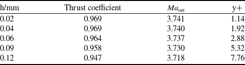
Performances at the outlet of nozzle vary with minimum spacing

Table 1 Long description
The table presents data on the performance at the outlet of a nozzle, varying with minimum spacing in millimeters. It contains five rows and four columns. The columns are labeled as follows: h/mm, Thrust coefficient, Ma out, and y+. The row data is as follows: Row 1: h/mm, 0.02; Thrust coefficient, 0.969; Ma out, 3.741; y+, 1.14. Row 2: h/mm, 0.04; Thrust coefficient, 0.969; Ma out, 3.740; y+, 1.92. Row 3: h/mm, 0.06; Thrust coefficient, 0.964; Ma out, 3.737; y+, 2.88. Row 4: h/mm, 0.09; Thrust coefficient, 0.958; Ma out, 3.730; y+, 5.32. Row 5: h/mm, 0.12; Thrust coefficient, 0.947; Ma out, 3.718; y+, 7.76. The table shows a trend where the thrust coefficient slightly decreases as the minimum spacing increases, while the y+ value increases with the minimum spacing.
3.3 Mesh independence verification
The grid independence study is conducted to determine the appropriate grid resolution, so different bottom mesh thicknesses (h = 0.02 mm, h = 0.04 mm, h = 0.06 mm, h = 0.09 mm, h = 0.12 mm) are selected to carry out the independence analysis of bottom mesh size. The performance parameters (treated by mass-weighted average, Ma = 6.0) on the nozzle exit by changing with the thickness of the bottom grid are listed in Table 1. It can be seen that the thrust coefficient and exit Mach number change greatly when h > 0.06 mm. Comparing with h = 0.02 mm and h = 0.04 mm, the thrust coefficient and exit Mach number are almost unchanged, which obviously meets the requirements of grid independence. Therefore, the bottom mesh size selected as calculation is performed on the grid of 0.04 mm (y +≍1.9).
In order to reduce the influence of mesh size on calculation results, three structured computational grids with different grid resolution, namely coarse (6,80,000 cells), medium (9,80,000 cells) and fine (1.34 million cells) grids, are generated for the nozzle designed by the proposed method. Figure 11 illustrates the mesh distributions at different grid densities, highlighting the refinement near the nozzle outlet, wall surfaces and shear layer regions used for the mesh independence verification. Under the inflow condition of Ma = 6.0, the pressure distribution on the down wall of different scale grids is shown in Fig. 12, from which it can be seen that the pressure distribution in a coarse grid has a large deviation compared with the other two-scale grids near
 $ x/L_{\textrm{ramp}} \approx 0.46 $
, while the pressure distribution of medium and fine is consistent. It is concluded that the numerical results are almost unaffected by the increase of mesh numbers when reaching 980,000. These results show that the medium grid resolution can be used to obtain an accurate result, which is adopted in the subsequent numerical simulations.
Mesh distributions at different grid densities for the mesh independence.

Figure 11 Long description
The image displays a detailed diagram illustrating mesh distributions at various grid densities for the purpose of achieving mesh independence in nozzle design. The diagram is divided into three sections labeled as Coarse, Middle, and Fine, each showing a different level of mesh density. The Coarse section features larger, less detailed grid cells, while the Middle section shows a more refined grid. The Fine section displays the most detailed and refined grid cells. Each section is magnified to highlight the mesh structure, with arrows indicating the transition from coarse to fine grids. The main image in the center shows a 3D model of a nozzle with a hexagonal mesh overlay, demonstrating the application of these grid densities on the nozzle surface. The diagram emphasizes the importance of grid refinement in achieving accurate and independent mesh results for nozzle design.
Pressure distribution on the ramp obtained from the different scale grids.

Figure 12 Long description
The line graph displays the pressure distribution on a ramp obtained from different scale grids. The x-axis represents the normalized distance along the ramp, while the y-axis shows the normalized pressure. Three lines are plotted: a solid red line for coarse grid, a dashed green line for middle grid, and a dotted blue line for fine grid. Two red circles highlight areas of interest where the lines diverge, with an arrow pointing to one of these circles, indicating a significant difference in pressure distribution among the grids.
3.4 Definitions of nozzle performance parameters
Parameters such as axial thrust coefficient C fx , lift coefficient C y and pitching moment M are important to quantify the nozzle performance. The axial thrust coefficient reflects the propulsion efficiency of the nozzle, while the lift and pitching moment play a vital role in balancing the head-up moment produced by the forebody and inlet.
The axial thrust F cx is calculated as:
 \begin{align} {F_{cx}} = \dot m{v_{inx}} + \left( {{p_{inx}} - {p_0}} \right){A_{{\rm{inx}}}} - {R_x}\end{align}
where v inx, p inx, A inx, p 0, R x are the nozzle entry axial velocity, static pressure, axial projection area of entry, ambient pressure and axial thrust, respectively.
The isentropic thrust of the nozzle is denoted as F s, which can be calculated as follows:
 \begin{align} {F_s} &= \dot m\sqrt {\frac{{2\gamma }}{{\gamma - 1}}R{T_t}\left( {1 - {{\left( {\frac{1}{\pi }} \right)}^{\frac{{\gamma - 1}}{\gamma }}}} \right)} \end{align}
 \begin{align} \pi &= {p_t}/{p_0} \end{align}
where R, T
t
, p
t
are the gas constant, total temperature, and total pressure, respectively.
 $ \pi $
is defined as pressure drop ratio of the nozzle.
Finally, C fx and C y are calculated as follows:
 \begin{align} {C_{fx}} &= \frac{{{F_{cx}}}}{{{F_s}}}\end{align}
 \begin{align} {C_y} &= \frac{{{F_y}}}{{{q_0}A}}\end{align}
where q 0 and F y , A are the dynamic pressure of free stream, lift, and maximum projected area along the axial direction.
The reference point of M is the centre of the nozzle entry.
4.0 Result and discussion
4.1 Comparative analysis of the nozzle characteristics based on 2D MOC and 3D MOC
In order to prove the superiority of the nozzle design method based on 3D MOC, the characteristics of the nozzle designed by 3D MOC are compared with those designed by traditional 2D MOC design. According to the design conditions shown in Table 2 and the constraint of the same length, the 3D SERN profile with specific heat is obtained based on 2D MOC and 3D MOC. As shown in Fig. 13, the exit cross-sectional profiles of the two nozzles exhibit slight differences from the front view, indicating that the axial projected area of the nozzle designed using the 3D MOC method is approximately 1.4% smaller than that of the nozzle obtained from the 2D MOC method. This result suggests a slightly more compact expansion contour in the three-dimensional design. Moreover, from the vertical and side view. the profile difference of two nozzles is mainly manifested in the circumferential wall, which is the superposition effect of streamline tracing in different parent flowfields and using reference temperature method.
Profile comparison of 3D SERN with specific heat based on 2D MOC and 3D MOC.

Figure 13 Long description
The image presents a comparison of 3D Supersonic Expanding-Ramp Nozzle (SERN) profiles based on two-dimensional and three-dimensional Method of Characteristics (MOC). The illustration includes three views: front, vertical, and side. Each view shows the nozzle profiles generated by the 2D MOC and 3D MOC methods. The front view displays the cross-sectional shapes of the nozzles, highlighting the differences in design between the two methods. The vertical view provides a side perspective, showing the length and curvature of the nozzles. The side view offers another lateral perspective, emphasizing the outlet shape and overall structure. The comparison illustrates how the 3D MOC method can achieve more flexible and optimized nozzle designs under specific geometric constraints.
Airflow condition of design point

Table 2 Long description
The table presents a comparison of airflow conditions at the design point, focusing on parameters such as Mach number, height, Mach number at inlet, temperature, and pressure. It consists of one row and five columns. The columns are labeled as Ma c, H/km, Ma in, Ti/K, and p1/kPa. The data in the row are as follows: Ma c is 6.0, H/km is 26.0 kilometers, Ma in is 1.68, Ti/K is 2430 kelvin, and p1/kPa is 389 kilopascals. This table provides a detailed comparison of the specified parameters under the given design conditions.
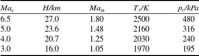
In addition to the airflow conditions listed in Table 2, two nozzles designed by 2D MOC and 3D MOC are numerically simulated under other typical flight conditions listed in Table 3. Figure 14 shows the performance comparison of the two nozzles under different flight Mach number, from which it can be seen that the performance of the two nozzles has the same change trend with the improvement of flight Mach number. The axial thrust coefficient decreases at first and then increases, which is minimum when Ma = 4.0 and reaches maximum when Ma = 6.5. Moreover, the lift coefficient first increased and then decreased, which reaches the maximum when Ma = 5.0. Compared with the nozzle designed by 2D MOC, the axial thrust coefficient of the nozzle designed by 3D MOC is increased by more than 0.45%. With the increase of the Mach number, the increment of the axial thrust coefficient first increases and then decreases, whose maximum increases are 0.675% at Ma = 4.0 and 0.467% at Ma = 6.0. The lift coefficient showed a substantial increase with increasing Mach number, except at Ma = 3.0, with increases of more than 13% observed in all other cases. Besides that, the lift coefficient increases with the increase of the flight Mach number, reaching the maximum value of 16.6% at Ma = 6.5 and increasing by 16.0% at Ma = 6.0.
Variation of axial thrust coefficient and lift coefficient with flight Mach number.

Figure 14 Long description
A two line graph showing the variation of axial thrust coefficient and lift coefficient with flight Mach number. The x axis represents the flight Mach number ranging from 3 to 6.5. The y axis on the left represents the axial thrust coefficient ranging from 0.58 to 0.68, and the y axis on the right represents the lift coefficient ranging from 0.05 to 0.09. The graph includes two data series: one for 2D MOC represented by blue triangles and another for 3D MOC represented by red squares. The axial thrust coefficient increases with the flight Mach number for both 2D MOC and 3D MOC, with 3D MOC generally showing higher values. The lift coefficient also increases with the flight Mach number, peaking around a flight Mach number of 5 for both 2D MOC and 3D MOC, with 3D MOC showing higher values throughout. All values are approximated.
Airflow conditions of typical flight Mach number

Table 3 Long description
The table presents airflow conditions for various flight Mach numbers, including Mach 6.5, 5.0, 4.0, and 3.0. It has four rows and four columns. The columns are labeled Ma, H/km, Ma_in, T/K, and p_t/kPa. Each row provides specific values for these parameters. For example, at Mach 6.5, the altitude is 27 kilometers, the inlet Mach number is 1.80, the temperature is 2500 Kelvin, and the total pressure is 480 kilopascals. The table highlights how these conditions change with different Mach numbers, showing variations in altitude, inlet Mach number, temperature, and total pressure.
Figure 15 shows the pressure contours of two nozzles based on 2D MOC and 3D MOC in the central section under a typical flight Mach number, in which the distance between the two red auxiliary dotted lines clearly marks the axial distance of the weak expansion wave on the upper wall of the two nozzles. It can be observed that the position of expansion waves from the entry of the upper wall to the exit of the lower wall move upstream in the flowfield with the decrease of the flight Mach number. Compared with the nozzle designed by 3D MOC, the position of expansive waves of the nozzle designed by 2D MOC is closer to the upstream in the flowfield, and the weak expansive wave is especially obvious. With the increase of the flight Mach number, the position interval of expansion waves on the upper wall of the two nozzles gradually increases and the shocks downstream of the nozzle exit is closer to the upstream in the flowfield at Ma = 3.0. Thus, the position change of the expansion waves and the shocks downstream of the nozzle has a significant influence on the flowfield. The position change of expansion waves along the axial direction will lead to the difference of the pressure at the same position of the nozzle, which will directly affect the effort of the airflow on the upper wall. This also explains why the nozzle designed by 3D MOC has better performance, and the increase of lift coefficient is particularly obvious.
Comparison of pressure distribution on the cross section between two nozzles.

Figure 15 Long description
A heat map comparing pressure distribution on the cross section between two nozzles at different Mach numbers. The heat map features a color scale ranging from blue to red, indicating pressure values from 0 to 110 kilopascals. The map is divided into two rows, each representing a different nozzle design: the 3D MOC and the 2D MOC. The columns represent different Mach numbers: 6.5, 5.0, 4.0, and 3.0. Each section of the heat map shows the pressure distribution around the nozzle cross sections, with higher pressure areas indicated by warmer colors and lower pressure areas by cooler colors. The red dashed lines in the middle of each section highlight specific regions of interest within the nozzles.
4.2 Influence of tracing profile on nozzle performance
Based on 3D MOC, the flowfield and performance of nozzle tracing by different profiles are further discussed. As Fig. 16 shows, the circular nozzle and the rectangular nozzle are great differences, which are obtained by the same area of the tracing profile under the design conditions in Table 2. It is noted that the upper wall of the rectangular nozzle forms an arc-curved surface, which appears short on the middle and long on the side, while the lower wall forms a unique sharp angle. For the convenience of the following description, the rectangular nozzle is denoted as Nozzle A and the circular nozzle is denoted as Nozzle B.
Aerodynamic configurations obtained from different entry profiles.

Figure 16 Long description
The image displays two aerodynamic configurations labeled as circle and square. The left configuration shows a smooth, elongated shape with a circular cross-section, while the right configuration features a more angular, elongated shape with a square cross-section. Both shapes are depicted in a three-dimensional perspective, highlighting their distinct geometric profiles.
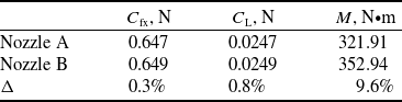
Table 4 shows performance comparison involved the axial thrust coefficient, lift coefficient and pitching moment of the two nozzles. It can be seen that compared with the difference of profiles, there is little difference in performance between two nozzles. The axial thrust coefficient and lift coefficient of Nozzle B are slightly improved compared to Nozzle A, while the pitching moment is improved with the increase reaching 9.6%. Figure 17 shows the pressure contours in the central section and isosurfaces of two nozzles, in which the red vertical auxiliary line is used to compare the position of the leading edge on the pressure isosurface near the upper wall. It can be seen that the pressure distribution of the two nozzles is similar, while there is a slight difference in the position of the pressure isosurface. Moreover, comparing with Nozzle A, the expansion of Nozzle B is slightly slower in the initial stage and faster in the downstream, which can be seen from the pressure isosurface from 36kPa to 6kPa. In addition, due to the difference of exit profiles, the shape of isosurface changes from almost the same to slightly different along the flow direction, especially there are obvious differences between Nozzle A and Nozzle B near the sharp corner on the exit of the lower wall. This is the reason why the lift and pitching moment of Nozzle B is higher than that of Nozzle A.
Comparative contour and isosurface of pressure in the central section of Nozzle A and Nozzle B.

Figure 17 Long description
A heat map comparing pressure distribution in Nozzle A and Nozzle B. The heat map features a color scale ranging from 0 to 90 kilopascals, with colors transitioning from blue (low pressure) to pink (high pressure). Nozzle A and Nozzle B are displayed side by side, each with a series of vertical red lines indicating specific pressure values. Nozzle A shows higher pressure values near the inlet, with a gradient decreasing towards the outlet. Nozzle B exhibits a more uniform pressure distribution along its length. The heat map highlights the differences in pressure contours and isosurfaces within the central sections of both nozzles, illustrating how pressure varies spatially within each nozzle design.
Performance comparison between Nozzle A and Nozzle B

Table 4 Long description
The table presents a performance comparison between Nozzle A and Nozzle B, focusing on three key metrics: axial thrust coefficient, lift coefficient, and pitching moment. It consists of three rows and four columns. The columns are labeled as C subscript f subscript x, N; C subscript L subscript 1, N; and M, N times m. The rows are labeled as Nozzle A, Nozzle B, and Delta. Nozzle A has an axial thrust coefficient of 0.647, a lift coefficient of 0.0247, and a pitching moment of 321.91 N times m. Nozzle B has an axial thrust coefficient of 0.649, a lift coefficient of 0.0249, and a pitching moment of 352.94 N times m. The Delta row shows a 0.3% improvement in axial thrust coefficient, a 0.8% improvement in lift coefficient, and a 9.6% improvement in pitching moment for Nozzle B compared to Nozzle A.
Compared with the profile of a conventional 2D rectangular nozzle, Nozzle A has some differences in upper and lower walls. In order to explore the differences in flowfield and performance between Nozzle A and the conventional 2D rectangular nozzle, three new nozzles are obtained by filling up the circular arc surface of the upper wall and the sharp corner of the lower wall on the basis of Nozzle A. As Fig. 18 shows, new nozzles are named Nozzle A-1, Nozzle A-2 and Nozzle A-3 in turns for convenience of description, among which Nozzle A-3 is similar to the profile of 2D rectangular nozzle with lateral expansion. The annotated ‘Fill-up’ regions indicate the modified wall surfaces relative to the baseline Nozzle A. The variations correspond to different filling positions on the upper and lower walls, illustrating how local geometric adjustments were applied to study their influence on the overall aerodynamic performance.
The profiles of new nozzles based on Nozzle A.

Figure 18 Long description
The illustration presents four different nozzle designs labeled as Nozzle A-1, Nozzle A-2, Nozzle A-3, and Nozzle A. Each nozzle design is depicted with a highlighted fill-up area, indicating regions where material or substance accumulates. The nozzles are shown in a side-by-side comparison, with arrows pointing to the specific areas of fill-up. The design variations suggest different structural or functional adaptations aimed at optimizing performance under specific conditions.
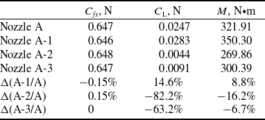
Comparing the performance of nozzles listed in Table 5, it can be seen that the change of upper and lower walls has relatively little influence on axial thrust. It is worth noting here that the axial thrust coefficient decreases and increases by 0.15%, respectively, after filling up the profile of upper and lower walls, while the axial thrust coefficient remains unchanged after filling up both (Nozzle A-3). Moreover, the influence of profile on lift and pitching moment is obvious that lift coefficient and pitching moment increase by 14.6% and 8.8%, respectively, when the profile of the upper wall is filled, decrease by 82.2% and 16.2%, respectively, when the profile of the lower wall is filled. So it can be seen that the profile to be filled has a great influence on the lift and pitching moment. Besides that, the lift coefficient and pitching moment of Nozzle A-3 are reduced by 63.2% and 6.7%, respectively, which shows that the sharp angle surface filled in the lower wall has greater influence on the lift and pitching moment.
Performance comparison between Nozzle A and three new nozzles

Table 5 Long description
The table presents a performance comparison between Nozzle A and three new nozzles, labeled Nozzle A-1, Nozzle A-2, and Nozzle A-3. It includes three columns: thrust coefficient (C_f, N), lift coefficient (C_L, N), and moment (M, N* m). The table has six rows, with the first three rows showing the performance metrics for each nozzle and the last three rows showing the percentage changes in these metrics compared to Nozzle A. Nozzle A has a thrust coefficient of 0.647, a lift coefficient of 0.0247, and a moment of 321.91. Nozzle A-1 has a thrust coefficient of 0.646, a lift coefficient of 0.0283, and a moment of 350.30. Nozzle A-2 has a thrust coefficient of 0.648, a lift coefficient of 0.0044, and a moment of 269.86. Nozzle A-3 has a thrust coefficient of 0.647, a lift coefficient of 0.0091, and a moment of 300.39. The percentage changes for Nozzle A-1 show a -0.15% change in thrust coefficient, a 14.6% increase in lift coefficient, and an 8.8% increase in moment. For Nozzle A-2, there is a 0.15% increase in thrust coefficient, an 82.2% decrease in lift coefficient, and a 16.2% decrease in moment. Nozzle A-3 shows no change in thrust coefficient, a 63.2% decrease in lift coefficient, and a 6.7% decrease in moment.
As Fig, 19 shows, when comparing Nozzle A with Nozzle A-1, it can be seen that the flowfield has little change after filling up the upper wall, which appears that the isosurface moves forward slightly on the upper wall, and the isosurface at the sharp corner of the lower wall moves upward and integrates with the isosurface of 6kPa. Comparing Nozzle A with Nozzle A-2, as displayed in Fig. 19, the lower wall to be filled directly affects the shape of the isosurface, whose position on the upper wall moves downstream and the range of movement increases continuously. The change of the surface and position can be clearly seen on the isosurface of 6kPa. Compared with Nozzle A-2 and Nozzle A-3, it can be seen that the flowfield changes little and the shape of isosurface changes slightly whose position on the upper wall moves slightly upstream approaching the isosurface of Nozzle A. Therefore, it is obtained that the change of the profile causes the intuitive change of the isosurface. The upper and lower walls to be filled mainly affects the position and shape of isosurface, which is finally reflected in the change of nozzle performance.
Comparative contour of pressure distribution in the central section of Nozzle A and three new nozzles.

Figure 19 Long description
The heat map displays the pressure distribution in the central section of Nozzle A and three new nozzles. The map uses a color gradient to represent pressure levels in kilopascals, ranging from 0 to 90. The x-axis represents the horizontal distance, while the y-axis represents the vertical distance. Each nozzle section is labeled as Nozzle A, Nozzle A-1, Nozzle A-2, and Nozzle A-3. The color scale at the top indicates pressure values, with blue representing lower pressure and pink representing higher pressure. Notable regions of high pressure are observed near the inlet of each nozzle, gradually decreasing towards the outlet. The heat map provides a comparative analysis of the pressure distribution across the different nozzle designs.
From the above results discussed, it can be seen that the axial thrust of the nozzle has little change after filling the profile, while the lift and pitching moment have great change, which can increase the selectivity for the nozzle design. According to the geometric limitations, lift requirements and moment matching requirements, the design of aerodynamic nozzle profile can be carried out flexibly.
4.3 Influence of tracing radius on nozzle performance
Based on Nozzle A and Nozzle B discussed in Section 4.2, the effects of the different tracing radius (r/R = 0.7, 0.8, 0.9) on the flowfield and performance of the nozzle ensuring the same entry area are further discussed according to the design conditions listed in Table 2. For the convenience of the following description, the newly generated nozzles are denoted as Nozzle A-r0.8, Nozzle A-r0.7, Nozzle B-r0.8 and Nozzle B-r0.8, respectively, according to the different tracing radius.
As shown in Fig. 20(a), the tracing radius can significantly affect the axial thrust coefficient and lift coefficient of Nozzle A and Nozzle B, which decrease with the increase of tracing radius. Compared with the case of r/R = 0.7, when r/R = 0.9, the axial thrust coefficients of the Nozzle A and Nozzle B are reduced by 0.8% and 0.6%, respectively, while the lift coefficients are reduced by 12.4% and 8.8%, respectively. It indicates that the change of the tracing radius has a dominant impact on the lift coefficient, and Nozzle A is more likely to be affected. Unlike the obvious decrease of the lift coefficient, as displayed in Fig. 20(b), the increase of the tracing radius only has a slight influence on the nose-down pitching moment. In addition, the nose-down pitching moment of Nozzle B slightly decreases and then increases with the change of the tracing radius, which also corresponds to the turning point of the lift coefficient when r/R = 0.8 shown in Fig. 20(a).
Variances of the nozzle performances with the increase of the tracing radius.

Figure 20 Long description
The line graph displays the variances of nozzle performances as the tracing radius increases. The x axis represents the ratio of the tracing radius to the radius, ranging from 0.7 to 0.9. The y axis on the left shows the axial thrust coefficient, ranging from 0.646 to 0.654, while the y axis on the right shows the lift coefficient, ranging from 0.025 to 0.03. The graph includes four data lines: Sqr-C_fx, Sqr-C_y, Cir-C_fx, and Cir-C_y, each represented by different symbols and colors. The Sqr-C_fx line, represented by green squares, shows a decreasing trend. The Sqr-C_y line, represented by green triangles, also shows a decreasing trend but at a different rate. The Cir-C_fx line, represented by red squares, shows a steeper decreasing trend. The Cir-C_y line, represented by red triangles, shows the steepest decreasing trend. All values are approximated.
The pressure contours of Nozzle A and Nozzle B with different tracing radii are displayed in Fig. 21(a), in which the red vertical auxiliary line has the same effect as mentioned in Section 4.2. By comparing Nozzle A, Nozzle A-r0.8 and Nozzle A-r0.7, it can be seen that the flowfield of the initial expansion section and the area of the lower wall has little change under different tracing radii, whose differences are mainly reflected in the position change of the isosurface on the upper wall. Furthermore, with the increase of the tracing radius, the isosurfaces at the upper wall from 6kPa to 24kPa move upstream and the amplitude increases continuously, and the shape of isosurfaces gradually widens after deflection to the side at the same time. Figure 21(b) shows the pressure comparison of flowfields among Nozzle B, Nozzle B-r0.8 and Nozzle B-r0.7, in which the position of the isosurface on the upper wall has the same trend as that shown in Figure 21(a) with the increase of tracing radius, while the movement amplitude decreases slightly. Compared with Figure 21(a), the isosurfaces in the initial expansion section and over the lower-wall region show significant differences, particularly in the exit region highlighted by the red ellipse on the lower wall, where the isosurface shape changes noticeably.
Comparative contour of pressure distribution in the central section of Nozzle A and Nozzle B with different tracing radii.

Figure 21 Long description
A heat map showing pressure distribution in the central section of Nozzle A and Nozzle B with different tracing radii. The heat map is divided into two columns, each representing a different nozzle type: Nozzle A on the left and Nozzle B on the right. Each column contains three subplots, each representing a different tracing radius: 0, 0.8, and 0.7. The pressure values range from 0 to 90 kilopascals, with a color scale indicating the pressure intensity. Higher pressure values are represented by warmer colors, such as red and pink, while lower pressure values are represented by cooler colors, such as blue and green. The subplots for Nozzle A show a gradual decrease in pressure from the inlet to the outlet, with the highest pressure values concentrated near the inlet. The subplots for Nozzle B show a similar trend, but with some variations in the pressure distribution due to the different tracing radii. The red lines in each subplot indicate the boundaries of the nozzle, and the red circles highlight specific areas of interest within the nozzle.
Therefore, it can be seen that the various radii leads to differences in the position and shape of the isosurface as well as the flowfield of the outlet. The position change of the isosurface on the upper wall has a slight influence on the axial thrust coefficient, but has a greater influence on the lift coefficient, which is consistent with the conclusion obtained from the analysis of the flowfield in Section 4.2. It is worth noting that as the tracing radius increases, the characteristic that the lift changes more while the nose-down pitching moment changes little adds flexibility to the nozzle design when considering the requirements of the lift and matching moment both.
5.0 Conclusion
This study proposes a three-dimensional nozzle design approach based on the 3D MOC to enhance aerodynamic performance. The proposed 3D MOC design method allows the nozzle to better preserve the true three-dimensional characteristics of the parent flowfield compared with the conventional 2D MOC approach. The flow structures and aerodynamic performances of nozzles designed by both methods were compared and analysed, followed by an investigation of different entry-tracing profiles and geometric radii.
The following conclusions are drawn:
-
(1) The main profile difference between the nozzles designed by 2D MOC and 3D MOC occurs along the circumferential wall. Under typical flight conditions, the expansion wave and shock structures in the 3D MOC–designed nozzle are shifted further downstream, leading to an increase of over 0.45% in axial thrust coefficient and more than 8% in lift coefficient.
-
(2) The comparison between the RN and CN shows that, while their overall flowfields are similar, the CN provides higher lift and pitching moment coefficients than the RN. Moreover, variations in the infill profiles based on the RN have little effect on axial thrust but significantly affect the lift and pitching moment, improving the design flexibility when considering integrated vehicle requirements.
-
(3) As the tracing radius increases, the lift coefficient of both RN and CN decreases noticeably, while the axial thrust and pitching moment change only slightly. These findings provide useful guidance for future nozzle designs that aim to balance lift generation and moment matching.
Acknowledgements
The authors gratefully acknowledge the financial supports by the funding project STS/MY-ZY-2020–005 provided from science and technology on Scramjet laboratory of CARDC in China.