Introduction
Sensitivity tests promise to increase the reliability of regression analyses. Their central idea is “that a coefficient of theoretical interest is robust to the extent that this coefficient exhibits a small range of variation to the presence or absence of other explanatory variables” (Hafner-Burton Reference Hafner-Burton2005, 687). We demonstrate that the validity of inferences derived from sensitivity tests is limited and largely depends on the definition of robustness. Our results also suggest that sensitivity tests should not be used to reject hypotheses or to justify empirical models. We also show that the most widely used definition of robustness, Sala-i-Martin’s (Reference Sala-i-Martin1997) variant of model averaging, is more likely to suffer from identifying false positives than the inferential rule it replaced, Leamer’s (Leamer 1978; Leamer Reference Leamer1985) extreme bounds, and Bayesian model averaging.
Until the early 1990s, sensitivity testing (Leamer Reference Leamer1978) was rarely used and the few published analyses attracted little attention. This situation changed with a double strike: at first Levine and Renelt showed that “very few economic variables are robustly correlated with cross-country growth rates (…)” (Reference Levine and Renelt1992, 959). Five years later and in the same journal, Xavier Sala-i-Martin demonstrated that “a substantial number of variables can be found to be robustly related to growth” (Reference Sala-i-Martin1997, 182). The differences in findings between Sala-i-Martin’s and Levine and Renelt’s analysis results from one simple change: while Levine and Renelt rely on the “extreme bounds” suggested by Leamer, Sala-i-Martin, who argues that this criterion “is too strong,” relies on a model averaging approach which, according to Sala-i-Martin, considers “the entire distribution of the estimators of β” (Sala-i-Martin Reference Sala-i-Martin1997, 179). Sala-i-Martin correctly understood the effect of using a less demanding inferential criterion: a more lenient robustness criterion identifies more, and potentially many more, variables as “robust.”Footnote 1 Yet, whether robustness tests that rely on Sala-i-Martin’s lenient criterion are more reliable—that is whether they avoid more false negatives and false positives—is an entirely different question—a question that Sala-i-Martin did not even try to answer.Footnote 2
This article offers the first systematic analysis of the reliability of inferential rules used in sensitivity testing. We rely on Monte Carlo analyses to analyze the ability of six different inferential rules—ranging from Leamer’s extreme bounds analysis to Bayesian model averaging—to distinguish “determinants,” i.e., variables included in the true model, from “confounders,” i.e., potential explanatory variables included in the sensitivity analysis that are not part of the true data-generating process. We show that inferential rules vary largely in their ability to avoid false positives and false negatives. In general, we can distinguish lax inferential rules, which are likely to identify determinants but seriously suffer from false positives and strict inferential rules, which are likely to reject confounders, but produce a large number of false negatives. Perhaps more importantly, our Monte Carlo analyses also demonstrate that no inferential rule avoids wrong judgments other than in trivial cases where a determinant exerts a strong and unconditional effect on the outcome and that determinant is only weakly correlated to confounders. As a result, sensitivity tests cannot be used reliably to specify an empirical model or to reject hypotheses. However, if a variable turns out to be robust based on a strict inferential rule, sensitivity tests may increase the certainty of an inference. Verification of hypotheses through sensitivity tests only works reliably, if the reliability of the inferential rule does not suffer from false positives. Two robustness definitions work best in this respect: extreme bounds and Bayesian model averaging. Both definitions of robustness allow researchers to identify explanatory factors which are unlikely not to influence the outcome.
The purpose and relevance of sensitivity tests
Empirical researchers usually do not know the true model. Therefore, they are likely to exclude variables which belong in the model and—at the same time—include variables which do not belong in the model. In other words: empirical models almost certainly suffer from model misspecifications that bias estimates and potentially invalidate inferences (Neumayer and Plümper Reference Neumayer and Plümper2017).
Model uncertainty invites model shopping and p-hacking. As Hafner-Burton suggests: “In conventional methods of reporting, we present the single best-fitting result, i.e., the result that best corresponds with our prior theoretical beliefs. We often arrive at this result through the exploration of several different models, including or excluding doubt variables from the regression until the model satisfies our theoretical standards” (Reference Hafner-Burton2005). Model uncertainty and the potential for fine-tuning empirical results to fit theoretical expectations create the ground for sensitivity analyses (Leamer 1978; Leamer Reference Leamer1985, Leamer and Leonard Reference Leamer and Leonard1983).
The key idea of sensitivity testing is that parameter estimates are not per se reliable because empirical models are likely to suffer from misspecification. One strategy of dealing with model uncertainty is to replace the representation of a single or a small number of carefully specified regression models by a large number of models randomly drawn from all possible, plausible model specifications. Sensitivity analyses thus attempt to “determine the range of estimates that the data could support given a precisely defined range of assumptions” (Leamer Reference Leamer2010, 37).
Leamer’s original suggestion to rely on an inclusive definition of the model space quickly becomes unfeasible: as the number of explanatory variables included in the model space increases, the number of combinations of these variables exponentially. In this situation, researchers can choose between two strategies: either they analyze a random draw of models from the model space of all plausible models, or, alternatively, they limit the size of the model space. Levine and Renelt (Reference Levine and Renelt1992) choose the second strategy and introduced the 1+3+3 rule: instead of analyzing all combinations of variables, they only studies models that included the variable of interest, three control “that belong into the model” and a random draw of three of the remaining control variables. For example, if researchers include 20 variables in the sensitivity test the number of possible variable combinations results in a bit more than 1 million models (220–1=1,048,575 models to be exact). If we instead use the 1+3+3 rule, the number of possible variable combinations reduces the original model space to (20–1–3)!/3!(20–1–3–3)!=560 different models for the variable of interest instead of roughly 1 million possible specifications.
Perhaps more importantly, the interpretation of a distribution of parameter estimates requires an inferential rule which allows researchers to decide whether the estimated effects of variables of interest are either “robust” or “sensitive.” Leamer (Reference Leamer1985) suggested the “extreme bounds” as criterion for “robustness.” The extreme bounds of a coefficient of interest are given by $\hat{\beta }_{{{\rm min}}} {\minus}2\hat{\sigma }$ as the lower and $\hat{\beta }_{{{\rm max}}} {\plus}2\hat{\sigma }$
 as the upper bound and thus reflect the variability of an estimate across all model specifications.
The use of extreme bounds analysis as an inferential rule quickly proved unpopular with researchers who did not like the fact that the majority of variables included in robustness tests proved to be sensitive to changes of the model specification. Sala-i-Martin (Reference Sala-i-Martin1997)—a growth empiricist—was not convinced by Levine and Renelt’s (Reference Levine and Renelt1992) finding that almost no variable frequently used in growth regressions was robust. The obvious way to increase the number of robust variables was to relax the criterion for robustness. Accordingly, Sala-i-Martin claimed that a simple variant of model averaging produces a larger number of robust findings. The strategy of relaxing the robustness criterion paid off: the number of sensitivity test increased significantly—and almost all of the sensitivity analyses conducted after the publication of Sala-i-Martin’s article relied on his model averaging variant. Yet, the increase in sensitivity tests occurred in the absence of knowledge about whether and to what degree sensitivity tests allow applied researchers to draw valid inferences. In fact, some scholars even claimed that the fact that Sala-i-Martin’s model averaging identifies more variables as robust than Leamer’s extreme bounds criterion “illustrates the advantages of applying the Sala-i-Martin approach” (Sturm, Berger and de Haan Reference Sturm, Berger and de Haan2005, 188).
It is perhaps not needless to argue that confirmation does not imply validity. A laxer inferential robustness criterion certainly increases the number of “robust” variables, but some, many, or even all of these seemingly robust variables can be “wrong positives”: variables that appear robust but do not belong into the model. In addition, it may also be that laxer inferential criteria reduce the propensity for wrong negatives by increasing the number of wrong positives. In fact, our Monte Carlo analyses, to which we turn now, demonstrates the existence of a trade-off between reducing the number of wrong positives and the number of wrong negatives.
Design of the Monte Carlo analysis
This section tests whether various variants of extreme bound analysis and model averaging approaches produce valid inferences. We analyze in how far sensitivity testing correctly identifies the true model given the various definitions of robustness. While we are dominantly interested in the absolute performance of the various inferential rules (and thus sensitivity analysis in general), we also compare the relative performance of the six inferential rules to each other. As indicator of the reliability of an inferential rule, we compute the probability of false negatives and false positives. A “false negative” is a variable that is incorrectly classified as “sensitive” when in fact it belongs in the true model specification. Conversely, a “false positive” is a variable that is incorrectly classified as “robust” when in fact it does not belong in the true model. Therefore, the probability of false negatives is 1 minus the average number of true positives divided by the number of determinants p. The probability of false positives is one minus the average number of true negatives divided by the number of confounders k−p.
We compare three extreme bounds algorithms and three model averaging techniques: Leamer’s (Reference Leamer1983) original extreme bounds technique (EBA_Leamer), that defines explanatory variables as “robust” if the minimum and maximum coefficient estimate both have the same sign and are both significant at the 0.05 significance level. This rule has been used by Levine and Renelt (Reference Levine and Renelt1992) and many others. A laxer variant of an extreme bounds analysis (EBA_Sign) only considers whether the minimum and the maximum coefficient estimates are of the same sign—regardless of whether they are significant or not. The third variant of extreme bound analysis (EBA_90) is even more lenient. It defines the extreme bounds not in terms of the minimum and maximum, but in terms of the 10 and 90 percent quantiles of the parameter distribution. Again, this test declares a variable robust if both are of the same sign. Our fourth algorithm (MA_Sala) is the widely used model averaging algorithm suggested by Sala-i-Martin (Reference Sala-i-Martin1997). It looks at the weighted average of the estimates and the weighted average of their respective variances, i.e.
 $$\widehat{\beta }_{{MA}} {\equals}\mathop{\sum}\limits_{j{\minus}1}^M {w_{j} } \widehat{\beta }_{j} \,{\rm and}\,\widehat{\sigma }_{{MA}}^{2} {\equals}\mathop{\sum}\limits_{j{\minus}1}^M {w_{j} } \widehat{\sigma }_{j}^{2}.$$
Sala-i-Martin used the integrated likelihoods as model weights to favor better fitting models in the averaging. That is, the weight for model m is given by
 $$w_{m} {\equals}{{L_{m} } \over {\mathop{\sum}\limits_{j{\minus}1}^M {L_{j} } }},$$
where L j denotes the likelihood of model j. He restricted robustness to variables whose coefficients were significantly different from 0 with a probability of 95 percent or more.Footnote 3 The fifth algorithm (MA_unif) is unweighted. In addition, next to the variance of the estimated coefficients it also considers the variance in estimates across different models, i.e.
 $$\sigma _{{MA}}^{2} {\equals}\mathop{\sum}\limits_{m{\minus}1}^M {w_{m} } \sigma _{m}^{2} {\plus}\mathop{\sum}\limits_{m{\minus}1}^M {w_{m} } \left( {\widehat{\beta }_{m} {\minus}{1 \over M}\mathop{\sum}\limits_{m{\minus}1}^1 {\widehat{\beta }_{m} } } \right)^{2}.$$
Finally, we include the standard Bayesian model averaging algorithm (MA_BIC), which weights coefficient estimates and variances by the Bayesian information criterion (Raftery Reference Raftery1995; Bartels Reference Bartels1997; Hoeting et al. Reference Hoeting, Madigan, Raftery and Volinsky1999). We can write this weight as
 $$w_{m} {\equals}{{e^{{\left( {{\minus}2\log \left( {L_{m} } \right){\plus}k_{m} \log \left( n \right)} \right)^{{\,/\,2}} }} } \over {\mathop{\sum}\limits_{j{\equals}1}^M {e^{{\left( {{\minus}2\log \left( {L_{j} } \right){\plus}k_{j} \log \left( n \right)} \right)^{{\,/\,2}} }} } }}.$$
In order to evaluate the performance of these inferential rules, we conduct several Monte Carlo experiments. All assumed data-generating processes in our Monte Carlo study take the general form of a simple linear model:
 $$y{\equals}\alpha {\plus}\mathop{\sum}\limits_{i{\equals}1}^P {x_{i} } \beta _{i} {\plus}e,$$
with normally distributed errors $e\,\sim\,N(0,\sigma )$ and where p stands for the number of variables included in the true model—we refer to these variables as “determinants”.
The total number of regressions that we estimated exceeds 46 million models. For each particular data generating process (DGP) we simulate a total of S=1000 data sets. Each data set has a size of N=1000 observations and contains a total of k potential explanatory variables $\left\{ {x_{1}, {\rm }x_{{2,}} \,\ldots\,,{\rm }x_{k} } \right\}$ (including the p determinants and k−p confounders). For each data set, and excluding the intercept-only model, one can now estimate 2
k
−1 possible model specifications,Footnote
4
yielding (2
k
−1)×1000 models per DGP. Determinants and confounders are randomly drawn from a multivariate normal distribution with mean 0 and specified covariance matrix. Assumptions on correlations differ between experiments and will be explained during the discussion of each experiment.
Results from Monte Carlo experiments
In this section we present the results of three Monte Carlo experiments and discuss the overall implications of these experiments in perspective.
Experiment 1: Sensitivity to uncorrelated confounders
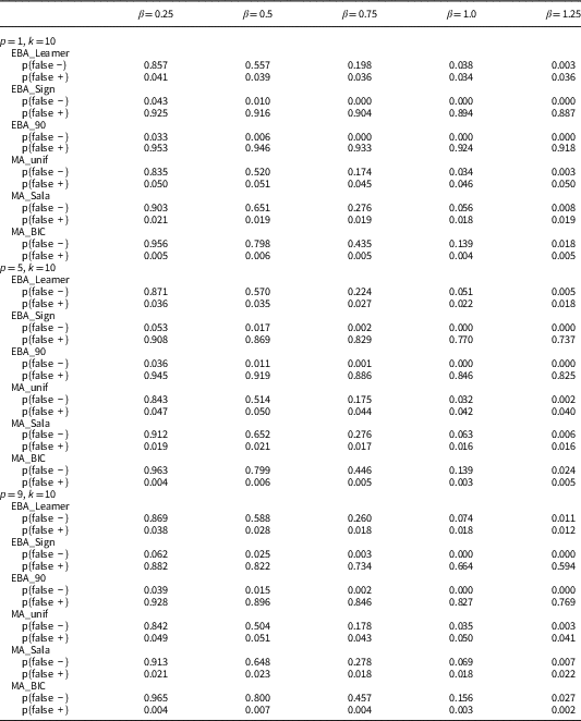
The first Monte Carlo experiment sets up DGPs to analyze the effects of the ratio of the number of true determinants p to the total number of potential variables k. Specifically, while k is always 10, we use various p from p={1, 5, 9}. We also vary the size of the coefficients β={0.25, 0.50, 0.75, 1.00, 1.25} of the true determinants (all p are assigned the same coefficient). The coefficient size is also a measure for the signal-to-noise ratio because we hold the residual standard deviation and the covariance structure constant so that $SE_{p} {\equals}\sigma \sqrt {(X^{'} X)_{{pp}}^{{{\minus}1}} } \,\approx\,0.25$ for all determinants.
In this first experiment we test the ability to separate true and false variables by assuming that the correlation between these variables is random and thus 0 on average. Arguably, this assumption is closer to the artificial world of econometric textbooks than to the real world of observational data. Although the assumption of uncorrelated variables makes the problem of separating “determinants” from “confounders” an easy task, inferential rules do not perform particularly well.
Table 1 reveals the following main results: Lax extreme bounds criteria (EBA_Sign and EBA_90) suffer from a high probability of false positives. In contrast, strict inferential rules are reliable in at least some experiments: Leamer’s extreme bounds and the three variants of model averaging perform well when the effects of the determinants are highly significant. In cases in which the certainty of the data remains low, strict inferential rules in sensitivity tests will generate a large number of false negatives.
Probability of False Positive and False Negatives When Variables are Uncorrelated

Note: Results based on S=1000 simulations per DGP. Results are optimal if p(false +) and p(false −) are both 0.0.
Experiment 2: Sensitivity to highly correlated confounders
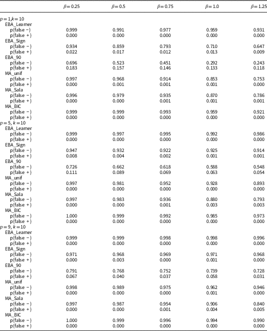
Experiment 2 turns the “soft assumption” of correlations made in experiment 1 upside down and randomly draws correlation from a uniform distribution with bounds at −0.99 and 0.99. This setting provides a much tougher test for sensitivity analysis. Arguably, experiment 2 leads to a lower share of false positives and a higher share of false negatives than any data-generating process that social scientists are likely encounter in real observational data. Table 2 presents the reliability of sensitivity analyses in this situation with weak separation between true and false variables. We find that, if we allow extreme correlations between determinants and confounders, the number of false negatives generated by all inferential rules skyrockets. Thus, the reliability of each inferential rule drops sharply. Under this condition, all inferential rules show a high tendency to characterize determinants as “not robust” even if they do in fact belong in the true data-generating process. In these situations, sensitivity tests are not at all reliable. One could be tempted to see the fact that false positives disappear with high correlations as an advantage. Unfortunately, this result is not helpful: with high correlations, sensitivity tests identify only very few variables as “robust”. In some cases, no variable turns out to be robust at all. For obvious reasons, a method that rejects all hypotheses and therefore yields no false positives, will not be very useful.
Probability of False Positive and False Negatives When Variables are Highly Correlated

Note: Results based on S=1000 simulations per DGP. Results are optimal if p(false +) and p(false −) are both 0.0.
Experiment 3: Sensitivity to the level of the correlation
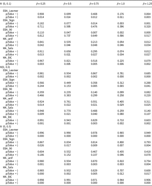
Our third experiment varies the correlations between ten potential variables (k=10). We always include five determinants (p=5), each with the same coefficient, which we vary across different simulations. We draw the correlational structures from normal distributions with mean 0 and different standard deviations, respectively [$r\,\sim\,N(0, .1)$ , $ \,\,r\,\sim\,N(0, .3)$
 , and $r\,\sim\,N(0, .5)$
 ]. The number of confounders is relatively large and variables are weakly to strongly correlated with confounders. The results of this experiment suggest that even weak correlations between variables can invalidate the inferences from sensitivity tests (see Table 3). Regardless of the exact inferential rule used, sensitivity tests are sensitive to correlations between determinants and confounders: when correlations reach levels common in observational data, not a single inferential rule turns out to be reliable. In fact, the probability of false negatives approaches 100 percent when researchers rely on Leamer’s extreme bounds rule and still lie between 60 and 100 percent when they use one of the model averaging approaches. It is also interesting to note that extreme bounds and model averaging rules respond differently to correlated confounders: whereas extreme bounds produce fewer false positives if confounders are correlated with determinants exerting a strong effect, model averaging algorithms generate fewer false positives if confounders are correlated with determinants exerting weak effects.
Probability of False Positive and False Negatives for Varying Levels of Correlation

Note: Results based on S=1000 simulations per DGP. Results are optimal if p(false +) and p(false −) are both 0.0.
Extensions: Heterogeneous effects and number of variables included in estimation model
We also ran a Monte Carlo experiment in which variables included in the true model have heterogeneous effect sizes. While in the previous experiments we assumed that all determinants have the same effect on the outcome, we now set the true coefficients as follows: β 1=0.25, β 2=0.5, β 3=0.75, β 4=1.0, β 5=1.25. Again, we experimented with different correlation structures. Obviously, the reliability of sensitivity tests depends on the strengths of effects and the number of variables with sufficiently strong effects. The higher the share of these strong determinants, the higher the total number of “robust” variables and, ultimately, the overall reliability of sensitivity tests. As the number of weak determinants increases, sensitivity tests quickly become unreliable.
Finally, we also analyze whether the performance of the inferential rules is influenced by the number of variables included in the empirical model. This analysis directly studies Levine and Renelt’s (Reference Levine and Renelt1992) conjecture that as the number of variables included in each estimation model increases (multi-) collinearity also increases, which ultimately invalidates inferences based on Leamer’s extreme bounds. We find that contrary to Levine and Renelt’s, Leamer’s extreme bounds criterion remains insensitive to the number of included variables in each model permutation. However, when scholars use a model averaging variant the number of positives—both false and true—increases as the number of variables included in models declines. As a consequence, the 1+3+3 rule does not seem to improve inferences based on extreme bounds, but it gradually helps with the validity of inferences based on model averaging.
Discussion
Social scientists conduct sensitivity tests because they are interested in the effect of a single variable on the outcome or because they hope sensitivity tests identify a good approximation of the true model. In the first case, sensitivity tests will find that the variable of interest is robustly related to the outcome if the relation between the variable of interest is strong, almost deterministic and unconditional. In addition, correlation between confounders and the variable of interest exert a strong influence on results of sensitivity tests and—as correlations become strong—largely diminishes the probability to find that the variable of interest is “robust.” If scholars use a 1+3+3 design, then the correlation between the variable of interest and the three always included controls has to be low to allow the variable of interest to become robust. If scholars use some uniform probability function for the inclusion of controls, the average correlation between the variable of interest and the confounders has to remain low. If the variable of interest has medium-sized positive and medium-sized correlation to controls, the odds are that sensitivity tests will not find that this variable of interest is robust.
In the second case, when researchers conduct a sensitivity test to improve the specification of the empirical model, not only the strengths of the variable of interest and the correlation between this variable and confounders matters. Instead, the strengths of all determinants and all cross-correlations influence the efficiency of the estimates, and thus the power of sensitivity testing. Ultimately, the empirical model identified by the sensitivity test will consist of fewer elements than the true model. Only the variables that exert the strongest effect, that are largely unconditional and uncorrelated with confounders tend to “survive” the sensitivity test. Social scientists should not expect that the model suggested by the sensitivity test mirrors the true model. We find that no inferential rule allows researchers to identify the true model and to reliably formulate inferences about regressors. A potential way to make correct inferences from sensitivity tests depends on using a strict inferential rule—Leamer’s extreme bounds or Bayesian model averaging—and to exclusively make inferences about the variables found to be robust. These are very likely included in the true model. Note that the opposite is not the case. Under no circumstances do sensitivity tests allow to reject hypotheses. This is so because no inferential rule can avoid false negatives.
Conclusion
Social scientists need to be cautious in using sensitivity tests for making inferences. Most importantly, results of sensitivity tests should not inform the specification of empirical models and should not be used to reject hypotheses. These are important results that hopefully precaution the consumers of sensitivity tests. Our Monte Carlo analyses generate crucial insights for the producers of sensitivity test. We have demonstrated that the definition of robustness on which the majority of social scientist relies, Sala-i-Martin’s model averaging, generates significantly more false positives than Leamer’s extreme bounds and Bayesian model averaging. That these criteria do at times identify more false negatives can be accepted because all procedures label many more variables as “sensitive” than they should. In other words, variables characterized as sensitive may easily belong into the empirical model.
Accordingly, sensitivity tests can increase the certainty of social scientists when (a) they rely upon strict inferential rules and (b) find that a variable is robust. In this case, the odds are good that the variable in fact belongs in the true model. This is so because strict inferential rules—Leamer’s extreme bounds and versions of Bayesian model averaging—have an extremely low probability of producing wrong positives. Hence, if social scientists rely on strict definitions of robustness and if a variable turns out to be robust, it is likely to belong into the empirical model.
Acknowledgments
A previous version of this paper was presented at the 6th Annual General Conference of the European Political Science Association (EPSA) in Brussels, 2016. The authors thank panel participants, two anonymous reviewers, and the former editor of PSRM, Vera Troeger, for comments and critique.