2 Preliminaries

We consider a uniformly stratified incompressible Boussinesq fluid with Brunt–Väisälä frequency $N_{0}>0$ on an $f$ -plane in Cartesian coordinates $(x,y,z)$ , rotating around the vertical axis $z$ with half the Coriolis frequency $f_{0}>0$ , and where gravity points along the negative $z$ -direction. In such rotating stratified fluids, inviscid internal waves with frequencies $\unicode[STIX]{x1D714}_{0}>0$ propagate at angle $\unicode[STIX]{x1D703}=\arctan \!\sqrt{(\unicode[STIX]{x1D714}_{0}^{2}-f_{0}^{2})/(N_{0}^{2}-\unicode[STIX]{x1D714}_{0}^{2})}$ with respect to the horizontal if either $f_{0}<\unicode[STIX]{x1D714}_{0}<N_{0}$ or $N_{0}<\unicode[STIX]{x1D714}_{0}<f_{0}$ . 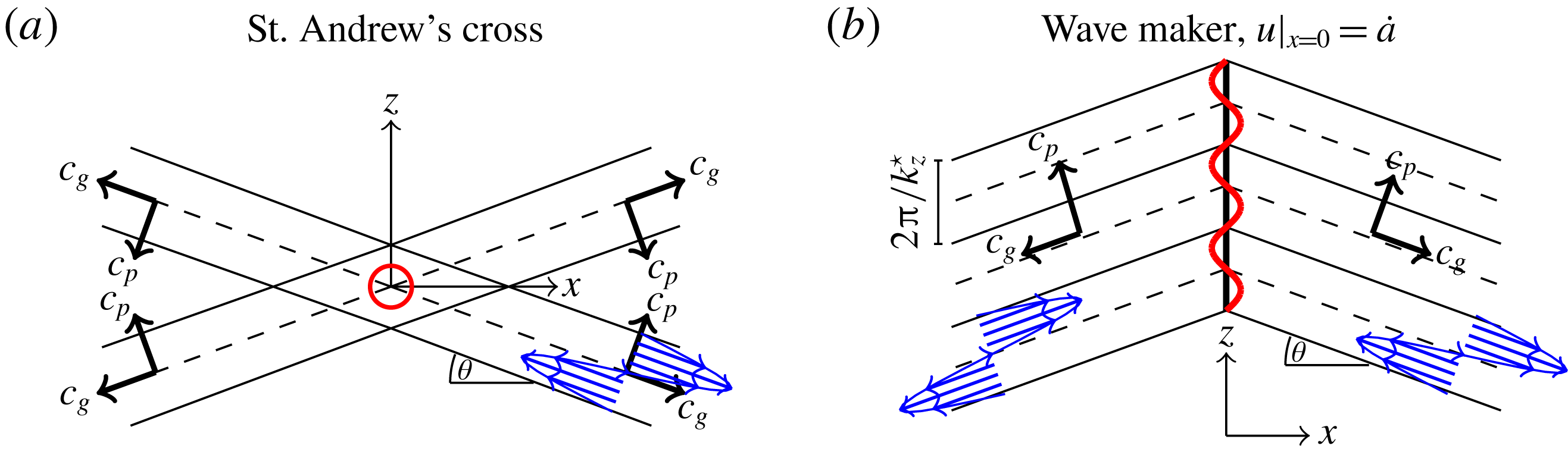For localized energy sources oscillating at frequency $\unicode[STIX]{x1D714}_{0}$ , this leads in two dimensions to the well-known St Andrew’s Cross (e.g. Sutherland (Reference Sutherland2010), also sketched in figure 1 a), and in three dimensions to double cones (Voisin Reference Voisin2003). Throughout this article, we consider boundary forcings at a vertical sheet, oscillating at frequency $\unicode[STIX]{x1D714}_{0}$ , representative of small-amplitude wall oscillations, such as sketched in figure 1(b). The precise oscillating boundary formulation is described in § 3.

Figure 1.

(a) Schematic snapshot of a St Andrew’s Cross generated by vertical oscillation of a line force (point source in $(x,z)$ -plane);  $c_{p}$ and $c_{g}$ indicate phase and group velocities. (b) Two wave beams generated by horizontal wave maker oscillations. We impose the horizontal velocity, ${\dot{a}}$ , of the oscillating wave maker (red line) at the centreline, $x=0$ (thick black line).

We shall work with dimensionless variables, employing some characteristic wavelength $L_{0}$ as length scale, $1/\unicode[STIX]{x1D714}_{0}$ as the time scale and $U_{0}=a_{0}\unicode[STIX]{x1D714}_{0}=\unicode[STIX]{x1D716}L_{0}\unicode[STIX]{x1D714}_{0}$ as the velocity scale, where $a_{0}$ is the dimensional wave amplitude and $\unicode[STIX]{x1D716}=a_{0}/L_{0}\ll 1$ is the Stokes number.

The governing equations for the non-dimensional velocity vector $\boldsymbol{u}=[u,v,w]$ , the buoyancy $b$ and the pressure $p$ with dimensionless Brunt–Väisälä frequency $N=N_{0}/\unicode[STIX]{x1D714}_{0}$ and Coriolis frequency $f=f_{0}/\unicode[STIX]{x1D714}_{0}$ in subscript-derivative notation are

(2.1) $$\begin{eqnarray}\displaystyle & \displaystyle \boldsymbol{u}_{t}+\unicode[STIX]{x1D716}(\boldsymbol{u}\boldsymbol{\cdot }\unicode[STIX]{x1D735})\boldsymbol{u}+f\hat{z}\wedge \boldsymbol{u}=-\unicode[STIX]{x1D735}p+\unicode[STIX]{x1D717}\unicode[STIX]{x0394}\boldsymbol{u}+\hat{z}b, & \displaystyle\end{eqnarray}$$

(2.2) $$\begin{eqnarray}\displaystyle & \displaystyle b_{t}+\unicode[STIX]{x1D716}\boldsymbol{u}\boldsymbol{\cdot }\unicode[STIX]{x1D735}b=-N^{2}w, & \displaystyle\end{eqnarray}$$

(2.3) $$\begin{eqnarray}\displaystyle & \displaystyle \unicode[STIX]{x1D735}\boldsymbol{\cdot }\boldsymbol{u}=0. & \displaystyle\end{eqnarray}$$

Here, $\unicode[STIX]{x1D717}=\unicode[STIX]{x1D708}/(\unicode[STIX]{x1D714}_{0}L_{0}^{2})$ , with $\unicode[STIX]{x1D708}$ the kinematic viscosity constant, and $\unicode[STIX]{x1D717}/\unicode[STIX]{x1D716}$ is the inverse Reynolds number. We assume both $\unicode[STIX]{x1D716}$ and $\unicode[STIX]{x1D717}$ to be small, allowing us to perform a perturbational expansion in these parameters.

We proceed by employing the wave/vortex decomposition for the horizontal flow (Staquet & Riley Reference Staquet and Riley1989; Voisin Reference Voisin2003). The Helmholtz decomposition thus reads

(2.4) $$\begin{eqnarray}\displaystyle \boldsymbol{u}=\unicode[STIX]{x1D735}_{h}\unicode[STIX]{x1D719}+\hat{z}\wedge \unicode[STIX]{x1D735}\unicode[STIX]{x1D6F9}+\hat{z}w, & & \displaystyle\end{eqnarray}$$

where $\unicode[STIX]{x1D719}$ is the potential (wave), and $\unicode[STIX]{x1D6F9}$ is the streamfunction (vortex) of the horizontal velocity. The usefulness of this decomposition relies on the absence of vertical vorticity ( $\unicode[STIX]{x1D6FA}^{z}=\unicode[STIX]{x0394}_{h}\unicode[STIX]{x1D6F9}$ ) for internal gravity wave fields, i.e. the vortex streamfunction $\unicode[STIX]{x1D6F9}$ is not associated with internal wave motion. The decomposition (2.4) transforms the continuity equation (2.3) into

(2.5) $$\begin{eqnarray}\displaystyle \unicode[STIX]{x0394}_{h}\unicode[STIX]{x1D719}+w_{z}=0. & & \displaystyle\end{eqnarray}$$

The lower index $h$ denotes horizontal components only, i.e. $\unicode[STIX]{x1D735}_{h}=[\unicode[STIX]{x2202}_{x},\unicode[STIX]{x2202}_{y},0]$ , $\unicode[STIX]{x0394}_{h}=\unicode[STIX]{x1D6FB}_{h}^{2}$ .

The curl of the horizontal momentum equations in (2.1), $\hat{z}\wedge \unicode[STIX]{x1D735}$ , reduces to

(2.6) $$\begin{eqnarray}\displaystyle (\unicode[STIX]{x2202}_{t}-\unicode[STIX]{x1D717}\unicode[STIX]{x0394})\unicode[STIX]{x0394}_{h}\unicode[STIX]{x1D6F9}+f\unicode[STIX]{x0394}_{h}\unicode[STIX]{x1D719}=\unicode[STIX]{x1D716}R, & & \displaystyle\end{eqnarray}$$

where

(2.7) $$\begin{eqnarray}\displaystyle R & = & \displaystyle ((\boldsymbol{u}\boldsymbol{\cdot }\unicode[STIX]{x1D735})u)_{y}-((\boldsymbol{u}\boldsymbol{\cdot }\unicode[STIX]{x1D735})v)_{x}\nonumber\\ \displaystyle & = & \displaystyle \underbrace{J(w,\unicode[STIX]{x1D719}_{z})}_{\text{wave}{-}\text{wave}}+\underbrace{J(\unicode[STIX]{x1D6F9},\unicode[STIX]{x0394}_{h}\unicode[STIX]{x1D6F9})}_{\text{vortex}{-}\text{vortex}}+\underbrace{w_{z}\unicode[STIX]{x0394}_{h}\unicode[STIX]{x1D6F9}\!-\!(\unicode[STIX]{x1D735}_{h}w)\boldsymbol{\cdot }(\unicode[STIX]{x1D735}_{h}\unicode[STIX]{x1D6F9}_{z})\!-\!(\unicode[STIX]{x1D735}_{h}\unicode[STIX]{x1D719})\boldsymbol{\cdot }(\unicode[STIX]{x1D735}_{h}\unicode[STIX]{x0394}_{h}\unicode[STIX]{x1D6F9})-w\unicode[STIX]{x0394}_{h}\unicode[STIX]{x1D6F9}_{z}}_{\text{wave}{-}\text{vortex}},\nonumber\\ \displaystyle & & \displaystyle\end{eqnarray}$$

and $J(A,B)=A_{x}B_{y}-B_{x}A_{y}$ is the horizontal Jacobian. The vertical curl of the nonlinear horizontal advection terms, $R$ , constituting the mean vertical vorticity production upon time averaging over the wave period, is analysed in detail in § 5.

Similarly, the divergence of the horizontal momentum equations becomes

(2.8) $$\begin{eqnarray}\displaystyle (\unicode[STIX]{x2202}_{t}-\unicode[STIX]{x1D717}\unicode[STIX]{x0394})\unicode[STIX]{x0394}_{h}\unicode[STIX]{x1D719}-f\unicode[STIX]{x0394}_{h}\unicode[STIX]{x1D6F9}=-\unicode[STIX]{x0394}_{h}p+O(\unicode[STIX]{x1D716}). & & \displaystyle\end{eqnarray}$$

This allows us to relate the pressure $p$ to the horizontal wave and vortex components, $\unicode[STIX]{x1D719}$ and $\unicode[STIX]{x1D6F9}$ , respectively, through

(2.9) $$\begin{eqnarray}\displaystyle p=-(\unicode[STIX]{x2202}_{t}-\unicode[STIX]{x1D717}\unicode[STIX]{x0394})\unicode[STIX]{x1D719}+f\unicode[STIX]{x1D6F9}+\unicode[STIX]{x1D6F9}^{cf}+O(\unicode[STIX]{x1D716}), & & \displaystyle\end{eqnarray}$$

where curl-free streamfunction $\unicode[STIX]{x1D6F9}^{cf}$ is a harmonic gauge, satisfying $\unicode[STIX]{x0394}_{h}\unicode[STIX]{x1D6F9}^{cf}=0$ , and determined by appropriate boundary conditions.

Expressing the vertical momentum equation in terms of $w$ and $\unicode[STIX]{x1D719}$ by employing the buoyancy equation (2.2), (2.6) and (2.8) gives

(2.10) $$\begin{eqnarray}\displaystyle [(\unicode[STIX]{x2202}_{t}-\unicode[STIX]{x1D717}\unicode[STIX]{x0394})^{2}+f^{2}]\unicode[STIX]{x2202}_{t}\unicode[STIX]{x2202}_{z}\unicode[STIX]{x0394}_{h}\unicode[STIX]{x1D719}-[(\unicode[STIX]{x2202}_{t}-\unicode[STIX]{x1D717}\unicode[STIX]{x0394})\unicode[STIX]{x2202}_{t}+N^{2}](\unicode[STIX]{x2202}_{t}-\unicode[STIX]{x1D717}\unicode[STIX]{x0394})\unicode[STIX]{x0394}_{h}w=0+O(\unicode[STIX]{x1D716}). & & \displaystyle\end{eqnarray}$$

Using the continuity equation (2.5), we can reduce (2.10) to

(2.11) $$\begin{eqnarray}\displaystyle [(\unicode[STIX]{x2202}_{t}-\unicode[STIX]{x1D717}\unicode[STIX]{x0394})^{2}\unicode[STIX]{x2202}_{t}\unicode[STIX]{x0394}+f^{2}\unicode[STIX]{x2202}_{t}\unicode[STIX]{x2202}_{z}^{2}+N^{2}(\unicode[STIX]{x2202}_{t}-\unicode[STIX]{x1D717}\unicode[STIX]{x0394})\unicode[STIX]{x0394}_{h}]w=0+O(\unicode[STIX]{x1D716}). & & \displaystyle\end{eqnarray}$$

Next, we discuss and specify boundary constraints representative of small-amplitude wall oscillations, for which we derive analytic solutions to (2.11) and (2.6) up to $O(\unicode[STIX]{x1D717},\unicode[STIX]{x1D716}^{0})$ accuracy in § 4.

3 Mathematical representation of oscillating boundary forcing

The aim is to formulate an appropriate mathematical description of a boundary value problem which is (i) representative of a small-amplitude horizontally oscillating boundary, such as a wave maker in the laboratory set-up by Bordes et al. (Reference Bordes, Venaille, Joubaud, Odier and Dauxois2012), and (ii) suitable to solve the linearized equations (2.1)–(2.3) analytically. Reasonable simplifications are necessary because it is notoriously difficult to compute the wave field with velocity vector $\boldsymbol{u}$ satisfying the impermeability boundary condition at the oscillating wall,

(3.1) $$\begin{eqnarray}\displaystyle \frac{\text{d}}{\text{d}t}(x-\unicode[STIX]{x1D716}a(t,y,z))=0\quad \Longleftrightarrow \quad \boldsymbol{n}\boldsymbol{\cdot }\boldsymbol{u}|_{x=\unicode[STIX]{x1D716}a(y,z,t)}={\dot{a}}(y,z,t), & & \displaystyle\end{eqnarray}$$

where $\text{d}/\text{d}t=\unicode[STIX]{x2202}_{t}+\unicode[STIX]{x1D716}\boldsymbol{u}\boldsymbol{\cdot }\unicode[STIX]{x1D735}$ is the material derivative, and $\boldsymbol{n}=(1,-\unicode[STIX]{x1D716}\unicode[STIX]{x2202}_{y}a,-\unicode[STIX]{x1D716}\unicode[STIX]{x2202}_{z}a)$ is a vector normal to the oscillating boundary, $x=\unicode[STIX]{x1D716}a(y,z,t)$ .

For computational convenience we restrict our analysis to temporally monochromatic wall oscillations, with non-dimensional frequency $\unicode[STIX]{x1D714}=1$ . (For the ease of dimensionalizing our expressions, we denote the frequency $1$ by $\unicode[STIX]{x1D714}$ everywhere. For dimensional expressions, simply replace $\unicode[STIX]{x1D714}$ by $\unicode[STIX]{x1D714}_{0}$ and $\unicode[STIX]{x1D717}$ by $\unicode[STIX]{x1D708}$ everywhere.) A straightforward generalization of our results to almost-periodic wave fields follows by the theory developed in Krol (Reference Krol1991). We consider the phase propagation ( $c_{p}$ ) of the oscillating wall to be primarily upwards, such that the group velocity ( $c_{g}$ ) of the generated wave field is primarily downwards, as sketched in figure 1(b). Purely upward phase propagation is atypical for laboratory experiments; the relative strength of the upward-propagating field component for primarily downward-propagating beams is discussed in the appendix, § A.2.

A key simplification, valid for all small-amplitude oscillations ( $\unicode[STIX]{x1D716}\ll 1$ ), consists of prescribing the impermeability constraint (3.1) at $x=0$ instead of at $x=\unicode[STIX]{x1D716}a(y,z,t)$ . If, additionally, the forcing in the vertical sheet is spatially smooth ( $\unicode[STIX]{x2202}_{y}a,\unicode[STIX]{x2202}_{z}a\in O(1)$ ), then the constraint (3.1) at $O(\unicode[STIX]{x1D716}^{0})$ accuracy reduces to

(3.2) $$\begin{eqnarray}\displaystyle u|_{x=0}={\dot{a}}(y,z,t). & & \displaystyle\end{eqnarray}$$

The physical wave makers in laboratory set-ups, which we want to mimic mathematically, typically have sharp edges, where $\unicode[STIX]{x2202}_{y}a\gg 1$ , possibly $\unicode[STIX]{x2202}_{y}a\geqslant 1/\unicode[STIX]{x1D716}$ . This means that the constraint (3.1) cannot be simplified to (3.2), i.e. the product of $\unicode[STIX]{x1D716}(\unicode[STIX]{x2202}_{y}a)$ and $v|_{x=0}$ in (3.1) is non-negligible. Recall that the monochromatic wall motion, ${\dot{a}}$ , generates a wave field which oscillates predominantly at frequency $\unicode[STIX]{x1D714}=1$ . This means that the product of $\unicode[STIX]{x2202}_{y}a$ with the dominating first harmonic of $v|_{x=0}$ (both oscillating at frequency $\unicode[STIX]{x1D714}$ ) results in a mean and/or second harmonic, which cannot be balanced by ${\dot{a}}$ or the first harmonic of $\boldsymbol{u}$ . An unphysical blow-up of mean and/or second harmonics at the lateral edges of the wave maker is only circumvented if $v|_{x=0}=0$ where $\unicode[STIX]{x2202}_{y}a\gg 1$ , and we are forced to add this condition as a constraint. While the impermeability constraint (3.1) cannot be reduced to constraint (3.2), we can reduce it to

(3.3a,b ) $$\begin{eqnarray}\displaystyle u|_{x=0}={\dot{a}}(y,z,t)\quad \text{everywhere},\quad \text{and}\quad v|_{x=0}=0\quad \text{where }\unicode[STIX]{x2202}_{y}a\gg 1. & & \displaystyle\end{eqnarray}$$

Similarly, we remark that where $\unicode[STIX]{x2202}_{z}a$ blows up, the vertical velocity should vanish ( $w|_{x=0}=0$ ). Treatment of this additional boundary forcing constraint is neglected because it is irrelevant for the main objective of the present analysis. (Large $\unicode[STIX]{x1D716}\unicode[STIX]{x2202}_{z}a$ corresponds to a horizontal line source, generating a St Andrew’s Cross, as sketched in figure 1(a), and discussed in §§ A.2 and 6. No separate treatment of $\unicode[STIX]{x1D716}\unicode[STIX]{x2202}_{z}a\gg 1$ is required because the present analysis, focusing on the vortical induced mean flow generation, is unaltered by the weak upward-propagating branch of the St Andrew’s Cross.) We emphasize that the constraint on $v$ in (3.3) belongs to the impermeability constraint, i.e. it does not specify a stress (no-slip) boundary condition for the along-wall velocity. This is important, because it implies that, even though $v$ points along the wall $x=0$ in our approximate description, we may not use a Stokes boundary layer solution for $v$ to satisfy (3.3).

Let us first discuss two common approaches to implement (3.2), before we discuss our implementation of (3.3).

The first approach consists in prescribing constraint (3.1) or a related formulation. This approach is popular in simulations because its numerical implementation is straightforward. For an idealized wave maker with no-stress boundary conditions, Raja (Reference Raja2018) prescribes $u(x=0)={\dot{a}}(t)$ . Using no-slip boundaries, Brouzet et al. (Reference Brouzet, Sibgatullin, Scolan, Ermanyuk and Dauxois2016) prescribe $w(x=0)=-{\dot{a}}(t)\tan \unicode[STIX]{x1D703}$ , which is equivalent to $u(x=0)={\dot{a}}(t)$ for two-dimensional (2D) inviscid wave beams that propagate under an inclination $\tan \unicode[STIX]{x1D703}$ . These representations of a wave maker generate an accurate internal wave far field, i.e. at sufficient distance from the energy input. However, our analysis in § 4 reveals that these implementations fail to describe the wave field components related to vertical line vortices, which are inevitably generated at the lateral edges of the wave maker. Those line vortices do play a significant role in the mean vertical vorticity production, and are thus essential for our analysis.

The second common approach consists in prescribing a momentum body forcing $\boldsymbol{F}=\hat{x}\ddot{a}(y,z,t)\unicode[STIX]{x1D6FF}(x)$ , where $\unicode[STIX]{x1D6FF}$ is the Dirac delta. This approach is popular in theoretical studies because Green’s functions of the governing equations are often known. For numerical implementations of this momentum-forcing approach, the Dirac delta is typically replaced by a sharp Gaussian. Although one can easily find equivalent body forcing formulations for forced boundary constraints for 2D problems, it appears non-trivial to do so for 3D problems.

We first solve the traditional boundary value constraint (3.2) approximately in terms of the wave potential ( $\unicode[STIX]{x1D719}$ ), such that we can subsequently construct a streamfunction $\unicode[STIX]{x1D6F9}$ to satisfy the additional constraint in (3.3) exactly. Although we are primarily interested in the half-open domain, $x>0$ , we naturally extend the analytical expressions to $\mathbb{R}^{3}$ by taking $u$ and $v$ even in $x$ , and $w$ odd in $x$ , as sketched in figure 1(b).

3.1 Wave maker representation

Throughout the remainder of this study, we consider

(3.4) $$\begin{eqnarray}\displaystyle a(y,z,t)=-E(y,z)\text{e}^{-\text{i}\unicode[STIX]{x1D714}t}\quad \text{with }E(y,z)=\frac{1}{4\unicode[STIX]{x03C0}^{2}}\int _{-\infty }^{\infty }\int _{0}^{\infty }\hat{E}(k_{y},k_{z})\text{e}^{\text{i}k_{y}y+\text{i}k_{z}z}\,\text{d}k_{z}\,\text{d}k_{y},\quad & & \displaystyle\end{eqnarray}$$

where the Fourier spectrum $\hat{E}$ of the normalized wall oscillation envelope is assumed to be negligible for all negative vertical wavenumbers $k_{z}$ to guarantee upward phase propagation, an assumption that can be dropped whenever needed. We work with complex expressions; physical quantities always correspond to the real part. For wave makers of height $2l_{z}$ , width $2l_{y}$ and vertical wavenumber $k_{z}^{\star }$ , we take

(3.5) $$\begin{eqnarray}\displaystyle \left.\begin{array}{@{}c@{}}\displaystyle E(y,z)=\unicode[STIX]{x1D6F1}_{c_{y},l_{y}}(y)\unicode[STIX]{x1D6F1}_{c_{z},l_{z}}(z)\exp [\text{i}k_{z}^{\star }z],\quad \unicode[STIX]{x1D6F1}_{c,l}(s)=\frac{\tanh [c(s+l)]-\tanh [c(s-l)]}{2},\\ \displaystyle \hat{E}(k_{y},k_{z})=\frac{\unicode[STIX]{x03C0}^{2}}{c_{y}c_{z}}\left(\sin [k_{y}l_{y}]\,\text{csch}\left[\frac{k_{y}\unicode[STIX]{x03C0}}{2c_{y}}\right]\right)\left(\sin [(k_{z}^{\star }-k_{z})l_{z}]\,\text{csch}\left[\frac{(k_{z}^{\star }-k_{z})\unicode[STIX]{x03C0}}{2c_{z}}\right]\right),\end{array}\right\} & & \displaystyle \nonumber\\ \displaystyle & & \displaystyle\end{eqnarray}$$

where the chosen smoothing parameters $c_{y}$ and $c_{z}$ must be sufficiently large, as discussed in detail in § 6, with the discontinuous edges corresponding to $c_{y}\rightarrow \infty$ and $c_{z}\rightarrow \infty$ . The exact solutions to the linearized equations, constructed in the next section, do not rely on this particular envelope choice, and thus are far more general.

4 Three-dimensional propagating internal wave beams

In this section, we construct analytic expressions for 3D internal wave fields generated by the oscillating boundary constraint, (3.3). Writing

(4.1) $$\begin{eqnarray}\displaystyle {\hat{W}}(x,k_{y},k_{z})=\int _{-\infty }^{\infty }\int _{-\infty }^{\infty }w(x,y,z,t)\exp [-\text{i}k_{y}y-\text{i}k_{z}z+\text{i}\unicode[STIX]{x1D714}t]\,\text{d}y\,\text{d}z, & & \displaystyle\end{eqnarray}$$

the governing equation (2.11) reduces to

(4.2) $$\begin{eqnarray}\displaystyle {\hat{W}}_{xx}+(k_{z}^{2}\unicode[STIX]{x1D707}^{2}-k_{y}^{2}){\hat{W}}=0, & & \displaystyle\end{eqnarray}$$

where

(4.3) $$\begin{eqnarray}\displaystyle \left.\begin{array}{@{}rcl@{}}\displaystyle \unicode[STIX]{x1D707}^{2}\; & =\; & \displaystyle \frac{\unicode[STIX]{x1D714}(-\text{i}\unicode[STIX]{x1D714}+\unicode[STIX]{x1D717}k^{2})^{2}+\unicode[STIX]{x1D714}f^{2}}{(\unicode[STIX]{x1D714}^{2}+\text{i}\unicode[STIX]{x1D714}\unicode[STIX]{x1D717}k^{2}-N^{2})(\unicode[STIX]{x1D714}+\text{i}\unicode[STIX]{x1D717}k^{2})}\\ \displaystyle \; & =\; & \displaystyle \tan ^{2}\unicode[STIX]{x1D703}+\text{i}\unicode[STIX]{x1D717}k^{2}\left(\frac{\unicode[STIX]{x1D714}^{2}N^{2}+f^{2}(N^{2}-2\unicode[STIX]{x1D714}^{2})}{\unicode[STIX]{x1D714}(N^{2}-\unicode[STIX]{x1D714}^{2})^{2}}\right)+O(\unicode[STIX]{x1D717}^{2}),\\ \displaystyle k\; & =\; & \displaystyle \frac{k_{z}}{\cos \unicode[STIX]{x1D703}}.\end{array}\right\} & & \displaystyle\end{eqnarray}$$

In deriving (4.2), we neglected $O(\unicode[STIX]{x1D717}^{2})$ terms by approximating the Fourier-transformed Laplace operator with $-k^{2}=-k_{z}^{2}/\cos ^{2}\unicode[STIX]{x1D703}$ whenever the Laplace operator is associated with viscous dissipation. The validity of this approximation will be apparent from the solution presented below, for which the Fourier-transformed Laplace operator becomes $-(k_{x}^{2}+k_{y}^{2}+k_{z}^{2})=-(\unicode[STIX]{x1D707}^{2}+1)k_{z}^{2}=-k^{2}+O(\unicode[STIX]{x1D717})$ , with $\unicode[STIX]{x1D707}$ given in (4.3).

The homogeneous solution of the 1D Helmholtz equation (4.2), which is bounded for $x>0$ , is proportional to $\exp [\text{i}k_{x}x]$ , where $k_{x}=\sqrt{k_{z}^{2}\unicode[STIX]{x1D707}^{2}-k_{y}^{2}}$ . This shows that the potential $\unicode[STIX]{x1D719}$ can be written as

(4.4) $$\begin{eqnarray}\displaystyle \unicode[STIX]{x1D719}(x,y,z,t)=\frac{1}{4\unicode[STIX]{x03C0}^{2}}\int _{-\infty }^{\infty }\int _{0}^{\infty }\hat{\unicode[STIX]{x1D719}}(k_{y},k_{z})\exp [\text{i}k_{x}x+\text{i}k_{y}y+\text{i}k_{z}z-\text{i}\unicode[STIX]{x1D714}t]\,\text{d}k_{y}\,\text{d}k_{z}, & & \displaystyle\end{eqnarray}$$

with the spectrum $\hat{\unicode[STIX]{x1D719}}(k_{y},k_{z})$ related to ${\hat{W}}(x,k_{y},k_{z})$ (by the continuity equation (2.5)) through

(4.5) $$\begin{eqnarray}\displaystyle \hat{\unicode[STIX]{x1D719}}(k_{y},k_{z})=\frac{\text{i}}{\unicode[STIX]{x1D707}^{2}k_{z}}{\hat{W}}(x,k_{y},k_{z})\exp [-\text{i}k_{x}x]. & & \displaystyle\end{eqnarray}$$

Without yet specifying the spectrum $\hat{\unicode[STIX]{x1D719}}(k_{y},k_{z})$ , we can readily write the 3D wave beam velocity field, which we denote by $\boldsymbol{u}^{b}$ , in terms of $\unicode[STIX]{x1D719}$ alone (up to $O(\unicode[STIX]{x1D717})$ accuracy):

(4.6a,b ) $$\begin{eqnarray}\displaystyle \boldsymbol{u}^{b}=\left(\begin{array}{@{}c@{}}u^{b}\\ v^{b}\\ w\end{array}\right)=\left(\begin{array}{@{}c@{}}\unicode[STIX]{x2202}_{x}\\ \unicode[STIX]{x2202}_{y}\\ -\!\tan ^{2}\unicode[STIX]{x1D703}\,\unicode[STIX]{x2202}_{z}\end{array}\right)\unicode[STIX]{x1D719}+\text{i}\unicode[STIX]{x1D717}\unicode[STIX]{x1D6FD}\left(\begin{array}{@{}c@{}}0\\ 0\\ \unicode[STIX]{x2202}_{zzz}\end{array}\right)\unicode[STIX]{x1D719},\quad \unicode[STIX]{x1D6FD}=\left(\frac{\unicode[STIX]{x1D714}^{2}N^{2}+f^{2}(N^{2}-2\unicode[STIX]{x1D714}^{2})}{\unicode[STIX]{x1D714}(N^{2}-\unicode[STIX]{x1D714}^{2})^{2}\cos ^{2}\unicode[STIX]{x1D703}}\right). & & \displaystyle \nonumber\\ \displaystyle & & \displaystyle\end{eqnarray}$$

The aim is to find a solution approximating the boundary forcing constraint (3.3). We start by considering constraint (3.2) and approximate $u|_{x=0}$ by $\text{i}k_{x}^{\star }\unicode[STIX]{x1D719}|_{x=0}$ , hence imposing

(4.7) $$\begin{eqnarray}\displaystyle \hat{\unicode[STIX]{x1D719}}=-\frac{\unicode[STIX]{x1D714}}{k_{x}^{\star }}\hat{E}(k_{y},k_{z}), & & \displaystyle\end{eqnarray}$$

where $k_{x}^{\star }=\tan \unicode[STIX]{x1D703}\,k_{z}^{\star }$ is the horizontal wavelength imposed by the wave maker. While approximating $u|_{x=0}$ by $\text{i}k_{x}^{\star }\unicode[STIX]{x1D719}|_{x=0}$ does imply a slight violation of the (already approximated) boundary constraint (3.3), it happens to come with the benefit of removing an unphysical singularity in $\unicode[STIX]{x2202}_{x}v$ at $(x,y)=(0,\pm l_{y})$ . (We remark that replacing $u|_{x=0}$ by $\text{i}k_{x}^{\star }\unicode[STIX]{x1D719}|_{x=0}$ also neglects the contribution from the curl-free streamfunction, $\unicode[STIX]{x1D6F9}^{cf}$ , determined below. Effectively, replacing $u|_{x=0}$ by $\text{i}k_{x}^{\star }\unicode[STIX]{x1D719}|_{x=0}$ boils down to approximating $\text{i}k_{x}+|k_{y}|=\text{i}\sqrt{\tan ^{2}\unicode[STIX]{x1D703}\,k_{z}^{2}-k_{y}^{2}}+|k_{y}|$ by $\text{i}\tan \unicode[STIX]{x1D703}\,k_{z}$ , valid for all sufficiently small $k_{y}$ , and then replacing $k_{z}$ by the imposed vertical wavenumber, $k_{z}^{\star }$ . The sharp spectral peaks at $k_{y}=0$ and $k_{z}=k_{z}^{\star }$ justify these simplifications.) Avoiding a singularity in $\unicode[STIX]{x2202}_{x}v$ at $(x,y)=(0,\pm l_{y})$ is essential because $v$ has to be continuous at $(x,y)=(0,\pm l_{y})$ in order to vanish at these edges.

Figure 3 illustrates the spatial structure of the (inviscid) $x$ -velocity component, $u^{b}$ , for the smoothed wave maker forcing profile depicted in figure 2.

Figure 2.

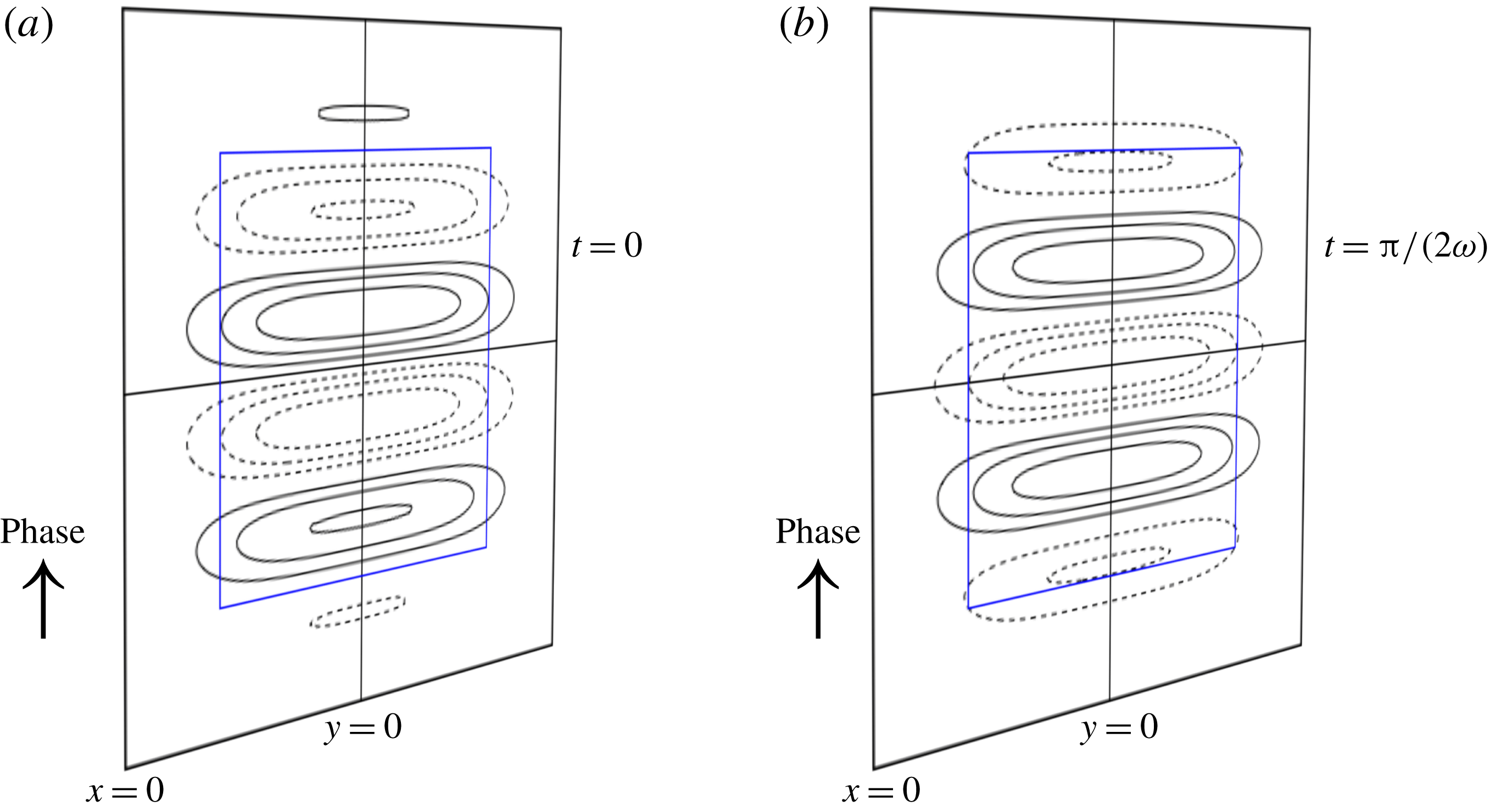
Sketch of the imposed boundary oscillation in the forcing plane $x=0$ , at two instances in time, (a) $t=0$ and (b) $t=\unicode[STIX]{x03C0}/(2\unicode[STIX]{x1D714})$ , for the smoothed wave maker envelope given by expression (3.5) with $c_{y}=c_{z}=2.5$ , $l_{y}=l_{z}=1$ and $k_{z}^{\star }=2\unicode[STIX]{x03C0}$ . The blue box indicates the wave maker domain, $(y,z)\in [-1,1]\times [-1,1]$ . The solid and dashed lines show contours of ${\dot{a}}(y,z,t)$ at $0.25$ intervals.

Figure 3.

The inviscid ( $\unicode[STIX]{x1D717}=0$ ) non-dimensional $x$ -velocity component, $u^{b}$ , of a 3D diffracting internal wave beam in three horizontal planes ( $z/l_{y}=0.3,~-1.2$ and $-2.7$ ), for the smoothed wave maker forcing depicted in figure 2. For clarity, values $|u|<0.05$ are invisible. The four blue diagonal dashed lines indicate the centre wave beam region (set by forcing region $(y/l_{y},z/l_{y})\in [-1,1]\times [-1,1]$ ). Owing to diffraction, the wave beam widens in the $y$ -direction with increasing distance to the source at $x=0$ .

The beam decays in the along-beam direction due to horizontal diffraction at rate $(1/\cos \unicode[STIX]{x1D703})\,\text{Im}[\sqrt{k_{z}^{2}\tan ^{2}\unicode[STIX]{x1D703}-k_{y}^{2}}]$ , which is dominated by those transverse wavenumbers $k_{y}$ that are slightly larger (in absolute value) than $\unicode[STIX]{x1D707}k_{z}=\sin \unicode[STIX]{x1D703}\,k+O(\unicode[STIX]{x1D717})$ . This means that part of the generated internal waves, namely those associated with the wavenumber pairs $(k_{y},k_{z})$ satisfying $|k_{y}/k_{z}|>\tan \unicode[STIX]{x1D703}$ , cannot leave the forcing plane, $x=0$ , due to diffraction. On the contrary, diffraction is practically absent if the imposed spectrum $\hat{E}(k_{y},k_{z})$ at $x=0$ practically vanishes for $k_{y}>k_{z}\tan \unicode[STIX]{x1D703}$ , which is the case for transversely very wide, quasi-2D beams. Interestingly, the diffraction decreases with angle $\unicode[STIX]{x1D703}$ , i.e. quasi-horizontal propagating beams diffract much stronger than quasi-vertically propagating beams.

The viscous attenuation rate per unit distance along the beam, i.e. the real part of $\text{i}k_{x}\cos \unicode[STIX]{x1D703}$ at viscous order $O(\unicode[STIX]{x1D717})$ , is given by $\unicode[STIX]{x1D717}k^{4}\sin \unicode[STIX]{x1D703}/(2Nk_{x}\cos \unicode[STIX]{x1D703})$ . For 2D beams satisfying $k_{x}=k\sin \unicode[STIX]{x1D703}+O(\unicode[STIX]{x1D717})$ , we recover the viscous attenuation rate $\unicode[STIX]{x1D717}k^{3}/(2N\cos \unicode[STIX]{x1D703})$ (Thomas & Stevenson Reference Thomas and Stevenson1973; Lighthill Reference Lighthill1978; Voisin Reference Voisin2003), which equals $1/(2\unicode[STIX]{x1D706}_{H}\cos \unicode[STIX]{x1D703})$ in the notation of Bordes et al. (Reference Bordes, Venaille, Joubaud, Odier and Dauxois2012).

What remains to be solved is the vorticity equation (2.6) for the horizontal streamfunction $\unicode[STIX]{x1D6F9}$ , such that $v=\unicode[STIX]{x2202}_{y}\unicode[STIX]{x1D719}+\unicode[STIX]{x2202}_{x}\unicode[STIX]{x1D6F9}$ vanishes at the sharp vertical edges of the wave maker, at $(x,y)=(0,\pm l_{y})$ . Straightforward analysis gives

(4.8) $$\begin{eqnarray}\displaystyle \unicode[STIX]{x1D6F9}(x,y,z,t)=\unicode[STIX]{x1D6F9}^{rot}+s\unicode[STIX]{x1D6F9}^{sb}+(1-s)\unicode[STIX]{x1D6F9}^{cf}, & & \displaystyle\end{eqnarray}$$

consisting of rotational, Stokes boundary layer and curl-free streamfunctions, with the relative contribution of the latter two determined by the parameter $s$ , as discussed below. The rotational streamfunction,

(4.9) $$\begin{eqnarray}\displaystyle \unicode[STIX]{x1D6F9}^{rot}=-\frac{\text{i}\,f}{\unicode[STIX]{x1D714}+\text{i}\unicode[STIX]{x1D717}k^{2}}\unicode[STIX]{x1D719}=\frac{f}{\unicode[STIX]{x1D714}^{2}}(-\text{i}\unicode[STIX]{x1D714}-\unicode[STIX]{x1D717}k^{2})\unicode[STIX]{x1D719}+O(\unicode[STIX]{x1D717}^{2}), & & \displaystyle\end{eqnarray}$$

solves (2.6) at $O(\unicode[STIX]{x1D716}^{0})$ for given $\unicode[STIX]{x1D719}$ . In contrast to the other streamfunction components, this is the only vortex component directly linked to the propagating wave beam ( $\unicode[STIX]{x1D719}$ ), and it may be attributed to the internal wave field. Evidently, the rotational streamfunction vanishes for non-rotating fluids, to which we restrict the analysis in § 5.

The Stokes boundary layer streamfunction,

(4.10) $$\begin{eqnarray}\displaystyle \left.\begin{array}{@{}c@{}}\displaystyle \unicode[STIX]{x1D6F9}^{sb}=\frac{\unicode[STIX]{x1D714}^{2}}{4\unicode[STIX]{x03C0}^{2}k_{x}^{\star }}\int _{-\infty }^{\infty }\int _{0}^{\infty }\frac{k_{y}\hat{E}(k_{y},k_{z})}{k_{x}^{sb}(\unicode[STIX]{x1D714}+\text{i}\unicode[STIX]{x1D717}k_{z}^{2})}\exp [\text{i}k_{x}^{sb}|x|+\text{i}k_{y}y+\text{i}k_{z}z-\text{i}\unicode[STIX]{x1D714}t]\,\text{d}k_{y}\,\text{d}k_{z},\\ \displaystyle k_{x}^{sb}=\sqrt{\text{i}\frac{\unicode[STIX]{x1D714}}{\unicode[STIX]{x1D717}}-k_{y}^{2}-k_{z}^{2}},\end{array}\right\}\quad & & \displaystyle\end{eqnarray}$$

is the solution of the viscous vertical vorticity equation (2.6), i.e.

(4.11) $$\begin{eqnarray}\displaystyle (\unicode[STIX]{x2202}_{t}-\unicode[STIX]{x1D717}\unicode[STIX]{x0394})\unicode[STIX]{x1D6FA}^{sb}=0,\quad \unicode[STIX]{x1D6FA}^{sb}=\unicode[STIX]{x0394}_{h}\unicode[STIX]{x1D6F9}^{sb}, & & \displaystyle\end{eqnarray}$$

with $\unicode[STIX]{x1D6FA}^{sb}$ the associated vertical vorticity, and satisfying $\unicode[STIX]{x2202}_{x}\unicode[STIX]{x1D6F9}^{sb}|_{x=0}=-\unicode[STIX]{x2202}_{y}\unicode[STIX]{x1D719}|_{x=0}+O(\unicode[STIX]{x1D717})$ . Similarly, the curl-free streamfunction,

(4.12) $$\begin{eqnarray}\displaystyle \unicode[STIX]{x1D6F9}^{cf}=\frac{\text{i}\unicode[STIX]{x1D714}}{4\unicode[STIX]{x03C0}^{2}k_{x}^{\star }}\int _{-\infty }^{\infty }\int _{0}^{\infty }\text{sign}[k_{y}]\hat{E}(k_{y},k_{z})\exp [\text{i}k_{y}y-|k_{y}|x+\text{i}k_{z}z-\text{i}\unicode[STIX]{x1D714}t]\,\text{d}k_{y}\,\text{d}k_{z}, & & \displaystyle\end{eqnarray}$$

is the solution to

(4.13) $$\begin{eqnarray}\displaystyle \unicode[STIX]{x0394}_{h}\unicode[STIX]{x1D6F9}^{cf}=0\quad \text{satisfying }\unicode[STIX]{x2202}_{x}\unicode[STIX]{x1D6F9}^{cf}|_{x=0}=-\unicode[STIX]{x2202}_{y}\unicode[STIX]{x1D719}|_{x=0}. & & \displaystyle\end{eqnarray}$$

For the wave makers with sharp edges (envelope (3.5) with $c_{y}=c_{z}=\infty$ ), expression (4.12) reduces to

(4.14) $$\begin{eqnarray}\displaystyle \left.\begin{array}{@{}c@{}}\displaystyle \unicode[STIX]{x1D6F9}^{cf}=-\frac{\unicode[STIX]{x1D714}}{2\unicode[STIX]{x03C0}k_{x}^{\star }}(\log (r^{-})-\log (r^{+}))\exp [\text{i}k_{z}^{\star }-\text{i}\unicode[STIX]{x1D714}t]\quad \text{for }|z|<l_{z},\\ \displaystyle r^{\pm }=\sqrt{x^{2}+(y\mp l_{y})^{2}}\quad \text{for }x>0.\end{array}\right\} & & \displaystyle\end{eqnarray}$$

Note that this curl-free streamfunction can be interpreted as originating from two vertical line vortices at $y=\pm l_{y}$ .

The undetermined parameter $s$ in (4.8) weighs the relative contribution of the (viscous) Stokes boundary layer and (inviscid) vertical line vortices. The $y$ -velocity component associated with the Stokes boundary layer, $v^{sb}=\unicode[STIX]{x2202}_{x}\unicode[STIX]{x1D6F9}^{sb}$ , takes amplitude $O(\unicode[STIX]{x1D717}^{-1/2})$ at the vertical sheet, $x=0$ , i.e. large for weak viscosity. If we impose a no-slip boundary constraint on $v$ at $x=0$ , then $sv^{sb}$ must be balanced by other $O(1)$ velocity components, implying $s\in O(\unicode[STIX]{x1D717}^{1/2})$ . For a free-slip (no-stress) boundary condition on $v$ , the parameter $s$ must be zero, because a Stokes boundary layer cannot be established at stress-free boundaries. This illustrates that representing the oscillating boundary by a free-slip or no-slip surface is insignificant for the mean flow generation, allowing us to choose $s=0$ and neglect viscous boundary layer effects for simplicity.

From here onwards, we restrict ourselves to non-rotating fluids ( $f=0$ ). Rotational effects on the generation of mean flow are worth investigating in a separate paper.

5 Streaming and inviscid mean flow generation

We are interested in the generation of mean flow, driven by the time-averaged nonlinear terms in the governing equations (2.1)–(2.3), known as the mean Reynolds stresses. The mean Reynolds stresses at $O(\unicode[STIX]{x1D716})$ arise from the products of $O(\unicode[STIX]{x1D716}^{0})$ solutions. This process is also referred to as ‘streaming’ when related to viscous attenuation of the wave field (Lighthill Reference Lighthill1978), in analogy to acoustic streaming, or as ‘rectification’ when pertaining to the mean field produced by periodic waves, as in tidal rectification (see § 6.6 in Grisouard & Bühler (Reference Grisouard and Bühler2012) and references therein).

The question we want to answer is the following. Which wave field components are essential in forcing the potentially energetic vortical induced mean flow? As mentioned earlier, the vortical induced mean flow is associated with mean vertical vorticity, which is the only vorticity component which can accumulate energy in the presence of stratification. Conveniently, the (accelerating) vortical and (non-accelerating) buoyancy advection-induced mean horizontal flow components can be disentangled through a Helmholtz decomposition,

(5.1a,b ) $$\begin{eqnarray}\displaystyle \bar{u}=\bar{\unicode[STIX]{x1D719}}_{x}-\bar{\unicode[STIX]{x1D6F9}}_{y},\quad \bar{v}=\bar{\unicode[STIX]{x1D719}}_{y}+\bar{\unicode[STIX]{x1D6F9}}_{x}, & & \displaystyle\end{eqnarray}$$

where the overbar denotes time averaging over one wave period, $T=2\unicode[STIX]{x03C0}/\unicode[STIX]{x1D714}$ . The vertical velocity component, $\bar{w}$ , is attributed entirely to the buoyancy advection-induced mean flow. We briefly discuss the buoyancy advection-induced mean flow, before analysing the generation mechanisms driving the resonantly growing vortical induced mean flow.

5.1 Buoyancy advection-induced mean flow

Balancing the time-independent terms in the buoyancy equation (2.2), one readily finds at $O(\unicode[STIX]{x1D716})$ the buoyancy advection-induced mean vertical flow,

(5.2) $$\begin{eqnarray}\displaystyle \bar{w}=-\frac{\unicode[STIX]{x1D716}}{N^{2}}\,\overline{\text{Re}[\boldsymbol{u}]\boldsymbol{\cdot }\text{Re}[\unicode[STIX]{x1D735}b]}=-\frac{\unicode[STIX]{x1D716}}{2N^{2}}\,\text{Re}[\boldsymbol{u}\boldsymbol{\cdot }\unicode[STIX]{x1D735}b^{\ast }]=-\frac{\unicode[STIX]{x1D716}}{2\unicode[STIX]{x1D714}}\,\text{Im}[\boldsymbol{u}\boldsymbol{\cdot }\unicode[STIX]{x1D735}w^{\ast }], & & \displaystyle\end{eqnarray}$$

where $^{\ast }$ denotes complex conjugate, and we used $b=-\text{i}(N^{2}/\unicode[STIX]{x1D714})w+O(\unicode[STIX]{x1D716})$ . Remarkably, the buoyancy advection-induced mean flow may also be non-zero for 3D inviscid wave beams, apparent from substituting (4.6) into (5.2),

(5.3) $$\begin{eqnarray}\displaystyle \bar{w} & = & \displaystyle \frac{\unicode[STIX]{x1D716}\tan ^{2}\unicode[STIX]{x1D703}}{2\unicode[STIX]{x1D714}}\,\text{Im}\left[\left(\begin{array}{@{}c@{}}-\unicode[STIX]{x1D735}_{h}\\ \tan ^{2}\unicode[STIX]{x1D703}\,\unicode[STIX]{x2202}_{z}\\ \end{array}\right)\unicode[STIX]{x1D719}\boldsymbol{\cdot }\unicode[STIX]{x1D735}\unicode[STIX]{x1D719}_{z}^{\ast }\right]+O(\unicode[STIX]{x1D717})\nonumber\\ \displaystyle & = & \displaystyle \frac{\unicode[STIX]{x1D716}}{2\unicode[STIX]{x1D714}}\,\text{Im}[\tan ^{2}\unicode[STIX]{x1D703}\,(uu_{z}^{\ast }+vv_{z}^{\ast })-ww_{z}^{\ast }]+O(\unicode[STIX]{x1D717}).\end{eqnarray}$$

This emphasizes the fundamental difference with 2D wave beams, which satisfy $w=\tan \unicode[STIX]{x1D703}\,u+O(\unicode[STIX]{x1D717})$ , $v=0$ , and hence solve the nonlinear equations identically in the absence of viscosity (McEwan Reference McEwan1973; Tabaei & Akylas Reference Tabaei and Akylas2003).

In the appendix, § A.1, we show that, not surprisingly, this Eulerian vertical mean flow is exactly opposed by the vertical Stokes drift, such that the net (Lagrangian) vertical particle transport vanishes.

The continuity equation relates the vertical induced mean flow to the horizontal buoyancy advection-induced mean flow, $[\bar{\unicode[STIX]{x1D719}}_{x},\bar{\unicode[STIX]{x1D719}}_{y}]$ ,

(5.4) $$\begin{eqnarray}\displaystyle \unicode[STIX]{x0394}_{h}\bar{\unicode[STIX]{x1D719}}=-\bar{w}_{z}. & & \displaystyle\end{eqnarray}$$

For 2D internal wave beams in the $(x,z)$ -plane, we recover the 2D induced mean flow, $(\bar{u},\bar{w})=(Q_{z},-Q_{x})$ , with $Q=-\int \bar{w}\,\text{d}x$ the mean streamfunction, corresponding to equation (2.10) of Kistovich & Chashechkin (Reference Kistovich and Chashechkin2001), as well as equation (3.10) of Tabaei & Akylas (Reference Tabaei and Akylas2003). (Note that, confusingly, Kistovich & Chashechkin (Reference Kistovich and Chashechkin2001) refer to the induced mean flow as Stokes drift. The apparent factor of 4 difference in their expression results from a slightly different definition of the streamfunction.) The mean perturbation on the background stratification, equation (2.12) of Kistovich & Chashechkin (Reference Kistovich and Chashechkin2001) and equation (3.11) of Tabaei & Akylas (Reference Tabaei and Akylas2003), is more generally given by

(5.5) $$\begin{eqnarray}\displaystyle \bar{b}=\unicode[STIX]{x1D716}\,\overline{\text{Re}[\boldsymbol{u}]\boldsymbol{\cdot }\text{Re}[\unicode[STIX]{x1D735}w]}=\frac{\unicode[STIX]{x1D716}}{2}\,\text{Re}[\boldsymbol{u}\boldsymbol{\cdot }\unicode[STIX]{x1D735}w^{\ast }]. & & \displaystyle\end{eqnarray}$$

For a 3D wave beam, the expression (5.2) for $\bar{w}$ depends on the transverse coordinate $y$ , and the 2D Poisson equation (5.4) must be solved. The scalar field $\bar{\unicode[STIX]{x1D719}}$ inherits the $O(\unicode[STIX]{x1D716})$ amplitude from $\bar{w}$ , and is thus weak at all times for weakly nonlinear internal wave beams.

5.2 Vortical induced mean flow

We now turn to the vortical induced mean flow, $[-\bar{\unicode[STIX]{x1D6F9}}_{y},\bar{\unicode[STIX]{x1D6F9}}_{x},0]$ , which is confined to the horizontal plane. It evolves slowly over the slow time scale $\unicode[STIX]{x1D70F}=\unicode[STIX]{x1D716}t$ , governed by time-averaged vertical vorticity equation (2.6) for $f=0$ :

(5.6) $$\begin{eqnarray}\displaystyle \left(\unicode[STIX]{x2202}_{\unicode[STIX]{x1D70F}}-\frac{\unicode[STIX]{x1D717}}{\unicode[STIX]{x1D716}}\unicode[STIX]{x0394}\right)\unicode[STIX]{x0394}_{h}\bar{\unicode[STIX]{x1D6F9}}=\overline{R}. & & \displaystyle\end{eqnarray}$$

As argued in § 4, we can neglect the contribution from a Stokes boundary layer. An additional term $(1/\unicode[STIX]{x1D716})f\bar{w}_{z}$ appears on the right-hand side of (5.6) if rotation ( $f\neq 0$ ) is included, resulting in considerably more complicated dynamics by coupling the buoyancy advection-induced mean flow ( $\bar{w}$ ) with the vortical induced mean flow ( $\bar{\unicode[STIX]{x1D6F9}}$ ).

5.2.1 Streaming in the absence of rotation

For wave fields in non-rotating fluids ( $\unicode[STIX]{x1D6F9}^{rot}=0$ ), the mean vertical vorticity production resulting from beam–beam interactions associated with viscous dissipation is given by

(5.7) $$\begin{eqnarray}\displaystyle \overline{R}^{b} & = & \displaystyle J\,\overline{(\text{Re}[w],\text{Re}[\unicode[STIX]{x1D719}_{z}])}=-\unicode[STIX]{x1D717}\tilde{\unicode[STIX]{x1D6FD}}J\,\overline{(\text{Im}[\unicode[STIX]{x1D719}_{zzz}],\text{Re}[\unicode[STIX]{x1D719}_{z}])}+O(\unicode[STIX]{x1D717}^{2})\nonumber\\ \displaystyle & = & \displaystyle \unicode[STIX]{x1D717}\frac{\tilde{\unicode[STIX]{x1D6FD}}}{2}\,\text{Im}[{u_{z}^{b}}^{\ast }v_{zzz}^{b}-{v_{z}^{b}}^{\ast }u_{zzz}^{b}]+O(\unicode[STIX]{x1D717}^{2}),\end{eqnarray}$$

where $\tilde{\unicode[STIX]{x1D6FD}}=\tan ^{2}\unicode[STIX]{x1D703}/(\unicode[STIX]{x1D714}\cos ^{4}\unicode[STIX]{x1D703})=\unicode[STIX]{x1D6FD}$ for $f=0$ . Physically, the generation of mean vertical vorticity can be understood as slight tilting of the purely horizontal wave beam vorticity vector by the wave beam velocity field. An illustrative discussion of vortex tilting (also known as vortex twisting) can be found in Hoskins (Reference Hoskins1997).

For internal wave beams with a dominant vertical wavenumber, say $k_{z}^{\star }$ , we may replace $\unicode[STIX]{x2202}_{z}\rightarrow \text{i}k_{z}^{\star }$ , reducing (5.7) to

(5.8) $$\begin{eqnarray}\displaystyle \bar{R}^{b}=-\unicode[STIX]{x1D717}\tilde{\unicode[STIX]{x1D6FD}}{k_{z}^{\star }}^{4}(u^{b}(T/4)v^{b}(0)-u^{b}(0)v^{b}(T/4))+O(\unicode[STIX]{x1D717}^{2}), & & \displaystyle\end{eqnarray}$$

where $[u^{b}(t),v^{b}(t)]=\text{Re}[\unicode[STIX]{x1D735}_{h}\unicode[STIX]{x1D719}]$ . This expression is particularly useful for laboratory experiments, where $k_{z}^{\star }$ is imposed by the wave maker, and for which time series of the horizontal velocity field, $[u(t),v(t)]$ , in a horizontal plane are typically acquired using particle image velocimetry (PIV). (PIV is an optical method of flow visualization, which detects the displacement of particles suspended in a fluid. If the particles are sufficiently small (in the sense of negligible particle inertia time scale with respect to the smallest relevant time scale of the experiment), then the particle motion is identical to the fluid parcel motion, and experimental PIV velocity fields correspond to the Lagrangian velocity of the fluid. PIV measurements only represent the Eulerian velocity field if the Stokes drift is negligible.) The wave beam velocity field $[u^{b}(t),v^{b}(t)]$ can be extracted from $[u(t),v(t)]$ by filtering at the forcing frequency and applying a (discrete) Helmholtz decomposition. Note that expression (5.8) is valid for truly 3D wave fields. For quasi-2D wave fields, for which $k_{x}\approx k^{\star }\sin \unicode[STIX]{x1D703}=k_{z}^{\star }\tan \unicode[STIX]{x1D703}$ , valid if $|k_{y}|\ll k_{z}^{\star }\tan \unicode[STIX]{x1D703}$ , we can interchange $\unicode[STIX]{x2202}_{z}$ with $\cot \unicode[STIX]{x1D703}\,\unicode[STIX]{x2202}_{x}$ , reducing (5.7) to

(5.9) $$\begin{eqnarray}\displaystyle \bar{R}^{b}=-\frac{\unicode[STIX]{x1D717}{k^{\star }}^{3}}{2N\cos ^{2}\unicode[STIX]{x1D703}}\unicode[STIX]{x2202}_{y}U^{2}+O(\unicode[STIX]{x1D717}^{2}), & & \displaystyle\end{eqnarray}$$

where $U=\sqrt{\unicode[STIX]{x1D719}_{x}\unicode[STIX]{x1D719}_{x}^{\ast }}$ is the $x$ -velocity amplitude of the wave beam. This approximate expression is identical with the mean vertical vorticity production term in equation (2.16) of Fan et al. (Reference Fan, Kataoka and Akylas2018). An expression proportional to the mean vertical vorticity production derived by Bordes et al. (Reference Bordes, Venaille, Joubaud, Odier and Dauxois2012) is found upon assuming variations of $U$ to be purely due to viscous attenuation, with rate $\unicode[STIX]{x1D717}{k^{\star }}^{3}/(2N)$ in the $x$ -direction, equal to $1/(2\unicode[STIX]{x1D706}_{H})$ in their notation. (The mean vertical vorticity production term in (A 18) in Bordes et al. (Reference Bordes, Venaille, Joubaud, Odier and Dauxois2012) is a factor of 2 smaller as compared to our expression and the expression by Fan et al. (Reference Fan, Kataoka and Akylas2018).)

Whereas previous derivations (Bordes et al. Reference Bordes, Venaille, Joubaud, Odier and Dauxois2012; Kataoka & Akylas Reference Kataoka and Akylas2015; Fan et al. Reference Fan, Kataoka and Akylas2018), resulting in an expression similar to (5.9) for quasi-2D wave beams, only stress the importance of horizontal cross-beam variations ( $\unicode[STIX]{x2202}_{y}U\neq 0$ ), our more general expression (5.8) links streaming to the elliptical wave motion in the horizontal plane. This new insight implies that streaming is maximized for (nearly) circular wave motion, when $u$ and $v$ are of similar magnitude and out of phase. Strong streaming may thus be expected where two internal wave beams (both propagating upwards or downwards) intersect obliquely, for example two beams with propagation in, respectively, the $x$ - and $y$ -directions. Configurations of truly oblique intersections of wave beams, where the angle between the horizontal propagation directions is not $0^{\circ }$ or $180^{\circ }$ , have not yet been studied, although it seems plausible that oblique interactions of wave beams, generated at and scattered by nearby topographic features, are common in the 3D oceans.

Figure 4.

Schematic snapshot of the downward-propagating wave beam (solid and dashed phase lines in centre plane, $y=0$ , and a horizontal plane) and the velocity $v^{cf}=\unicode[STIX]{x1D6F9}_{x}^{cf}$ (red and blue areas), associated with the vertical line vortices at the edges ( $y=\pm l_{y}$ ) of the wave maker (grey shading at $x=0$ gives $E$ , the strength of forcing $F$ ). Mean vertical vorticity production through $\bar{R}^{cf}$ , dominated by $(1/2)\,\text{Re}[w_{x}^{\ast }v_{z}^{cf}]$ , occurs primarily in the red and blue shaded areas. The strength of $\bar{R}^{cf}\propto \sin (k_{x}^{\star }x)/x$ decays radially from the wave maker edges, with sign changes imprinted by the horizontal beam wavenumber,  $k_{x}^{\star }$ .

5.2.2 Inviscid mean flow generation associated with vertical line vortices

We now focus on the interaction of the curl-free streamfunction $\unicode[STIX]{x1D6F9}^{cf}$ with the wave beam, possible only through the second wave–vortex interaction term in (2.7), and given by

(5.10) $$\begin{eqnarray}\displaystyle \bar{R}^{cf}=-\overline{(\unicode[STIX]{x1D735}_{h}w)\boldsymbol{\cdot }(\unicode[STIX]{x1D735}_{h}\unicode[STIX]{x1D6F9}_{z}^{cf})}=\tan ^{2}\unicode[STIX]{x1D703}\,\text{Re}[u_{z}^{b}v_{z}^{cf^{\ast }}-v_{z}^{b}u_{z}^{cf^{\ast }}]+O(\unicode[STIX]{x1D717}), & & \displaystyle\end{eqnarray}$$

where we used $w_{x}=-u_{z}\tan ^{2}\unicode[STIX]{x1D703}+O(\unicode[STIX]{x1D717})$ and $w_{y}=-v_{z}\tan ^{2}\unicode[STIX]{x1D703}+O(\unicode[STIX]{x1D717})$ for the second expression. This mean vertical vorticity production is particularly interesting, because it may be non-zero even in the absence of viscosity ( $\unicode[STIX]{x1D717}=0$ ). For wave beams with dominant vertical wavenumber, $k_{z}^{\star }$ , we can further simplify (5.10) to

(5.11) $$\begin{eqnarray}\displaystyle \bar{R}^{cf}={k_{z}^{\star }}^{2}\tan ^{2}\unicode[STIX]{x1D703}\mathop{\sum }_{t\in \{0,\,T/4\}}(u^{b}(t)v^{cf}(t)-v^{b}(t)u^{cf}(t))+O(\unicode[STIX]{x1D717}), & & \displaystyle\end{eqnarray}$$

where $[u^{cf}(t),v^{cf}(t)]=\text{Re}[-\unicode[STIX]{x1D6F9}_{y}^{cf},\unicode[STIX]{x1D6F9}_{x}^{cf}]$ . As with (5.8), this expression is also useful if the horizontal velocity field, $[u(t),v(t)]$ , is known in a horizontal plane, such as is often the case for laboratory experiments. For an experimental dataset, it is important to verify whether $[u^{cf}(t),v^{cf}(t)]$ , extracted from $\unicode[STIX]{x1D714}$ -filtered $[u(t),v(t)]$ through a Helmholtz decomposition, is indeed vertical-vorticity-free (within measurement uncertainty).

For wave makers with sharp edges at $y=\pm l_{y}$ , such as sketched in figure 4, the velocity field associated with the line vortices decays inversely proportional to the distance to the wave maker edges (see also explicit streamfunction solution $\unicode[STIX]{x1D6F9}^{cf}$ , equation (4.14)). Variations of the wave beam velocity field in a horizontal plane (and within the beam) are dominated by the horizontal beam wavenumber, $k_{x}^{\star }=k_{z}^{\star }\tan \unicode[STIX]{x1D703}$ . As a consequence, the mean vertical vorticity production near the edges $y=\pm l_{y}$ , dominated by $\bar{R}^{cf}\approx (1/2)\,\text{Re}[w_{x}^{\ast }v_{z}^{cf}]$ , is characterized by the sinc function ( $\sin (k_{x}^{\star }x)/(k_{x}^{\star }x)$ ), changing sign with increasing distance to the wave maker at rate $\unicode[STIX]{x03C0}/k_{x}^{\star }$ . This is unlike streaming, which does not change sign along the $x$ -direction, decaying with distance to the wave maker only due to the (weak) decay of the wave beam strength. This suggests that, near the line vortices, inviscid mean flow generation associated with the line vortices prevails, whereas streaming dominates at sufficient distance from the wave maker.

Figure 5.

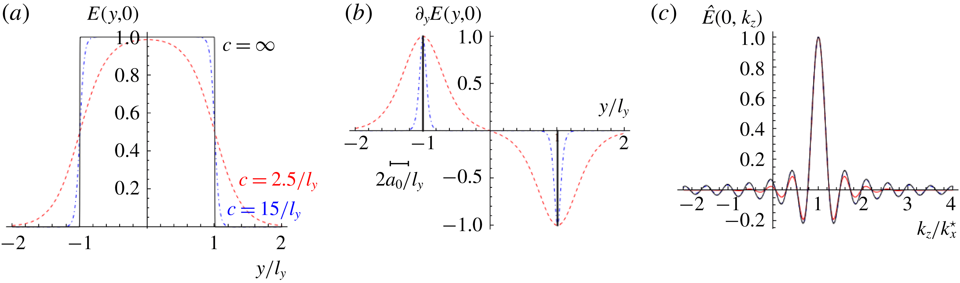
(a) The horizontal wave maker profile $E(y,0)$ , defined in (3.5); and (b) its derivative, $\unicode[STIX]{x2202}_{y}E(y,0)$ (normalized by its maximum), for $c_{y}=\infty$ (black, solid), our choice $c_{y}=15l_{y}^{-1}$ (blue, dot-dashed), and the choice by Kataoka & Akylas (Reference Kataoka and Akylas2015) and Fan et al. (Reference Fan, Kataoka and Akylas2018)  $c_{y}=2.5l_{y}^{-1}$ (red dashed). The vertical lines in (b) illustrate Dirac deltas; the horizontal line illustrates the relative wave maker excursion, $2a_{0}/l_{y}=0.27$ , in Bordes et al. (Reference Bordes, Venaille, Joubaud, Odier and Dauxois2012). (c) The spectrum $\hat{E}(0,k_{z})$ with $k_{z}^{\star }=3\unicode[STIX]{x03C0}/l_{z}$ for $c_{z}=\infty$ (black, solid), $c_{z}=15/l_{z}$ (blue, dot-dashed, almost indistinguishable) and $c_{z}=2.5/l_{z}$ (red, dashed).

6 Comparison with Bordes et al. (Reference Bordes, Venaille, Joubaud, Odier and Dauxois2012)

In this section, we compare our theoretical results with the experimental observations by Bordes et al. (Reference Bordes, Venaille, Joubaud, Odier and Dauxois2012). We adopt their parameter values, and specifically the wave frequency $\unicode[STIX]{x1D714}_{0}/N_{0}=0.26$ and wave maker amplitude $a_{0}=1$  cm corresponding to the experiments presented in their figures 2 and 3. We account for the wave maker inefficiency (Mercier et al. Reference Mercier, Martinand, Mathur, Gostiaux, Peacock and Dauxois2010) by reducing the wave maker amplitude for the theoretical expressions by 25 %. The associated Stokes number, $\unicode[STIX]{x1D716}=0.2$ , is sufficiently small for our perturbational expansion to be valid.

Imperfections in the laboratory set-up justify smooth approximations of the rectangular-shaped wave maker, i.e. finite smoothing parameters ( $c_{y}<\infty$ , $c_{z}<\infty$ ) in envelope function (3.5). A smooth envelope function $E(y,z)$ is needed to avoid the Gibbs phenomena when numerically integrating the wave beam field, expression (4.4). We find $c_{y}=c_{z}=15l_{y}^{-1}$ justifiable, because $\unicode[STIX]{x2202}_{y}E(y,0)\propto \unicode[STIX]{x2202}_{y}\unicode[STIX]{x1D6F1}_{c_{y},l_{y}}(y)$ then consists of two peaks with widths comparable to the wave maker excursion, $2a_{0}$ (see figure 5 b). This is not the case for the choice $c_{y}=2.5l^{-1}$ , made by Kataoka & Akylas (Reference Kataoka and Akylas2015) and Fan et al. (Reference Fan, Kataoka and Akylas2018), also illustrated in figure 5. (Whereas the rectangular-shaped wave maker was horizontally highly smoothed for numerical convenience, Kataoka & Akylas (Reference Kataoka and Akylas2015) and Fan et al. (Reference Fan, Kataoka and Akylas2018) did use sharp vertical envelopes, respectively $c_{z}=\infty$ and $c_{z}=7.5/l_{z}$ . It should be noted that they use $Y$ for the vertical and $Z$ for the transverse horizontal coordinate.)

Figure 6.

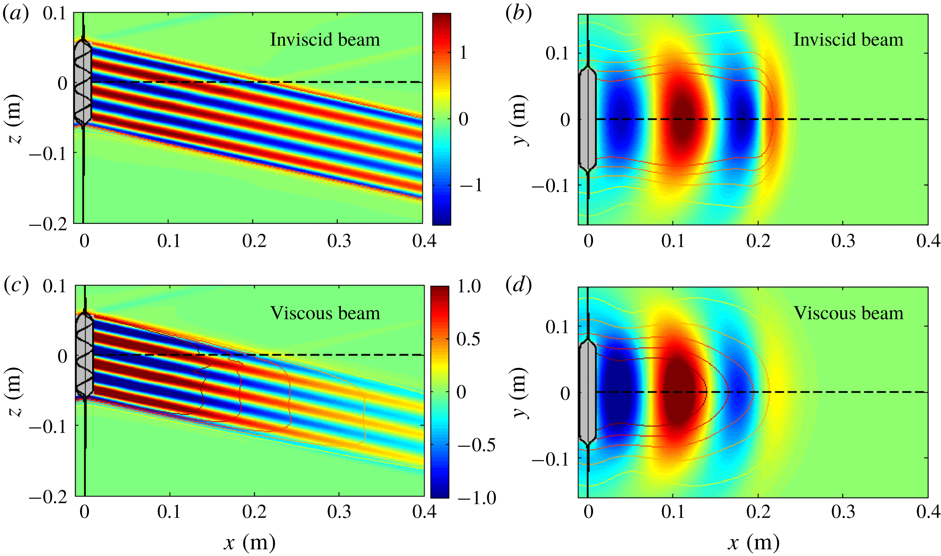
Snapshot of inviscid (a,b) and viscous (c,d) wave field velocity, $u(t)=\text{Re}[u]$ at $t=\unicode[STIX]{x03C0}$ , in $\text{mm}~\text{s}^{-1}$ , with contours representing the amplitude ( $|u|$ ). Panels (a,c) present the side view ( $y=0$ , dashed line in b,d) and panels (b,d) present the top view ( $z=0$ , dashed line in a,c). The plots are prepared so as to facilitate direct comparison with the experimental results in figure 2(a,b) of Bordes et al. (Reference Bordes, Venaille, Joubaud, Odier and Dauxois2012). The idealized wave maker envelope ( $c_{y}=c_{z}=15l_{y}^{-1}$ ) is indicated by the black lines. Grey area: extent of oscillating wave maker in laboratory set-up.

Figure 7.

Transverse horizontal ( $y$ ) velocity components in top view ( $z=0$ ) of (a) the wave beam, $v^{b}$ , (b) the line vortices, $v^{cf}$ , and (c) their sum, $v$ , in $\text{mm}~\text{s}^{-1}$ at $t=\unicode[STIX]{x03C0}$ , with contours representing their amplitude. All parameter values are as in figure 6. The colour bar shown in (b) applies to (a) and (c) too. The wave maker extent (grey area) is transparent, to visualize the singularities of $v^{b}$ and $v^{cf}$ at the edges, absent for $v$ . 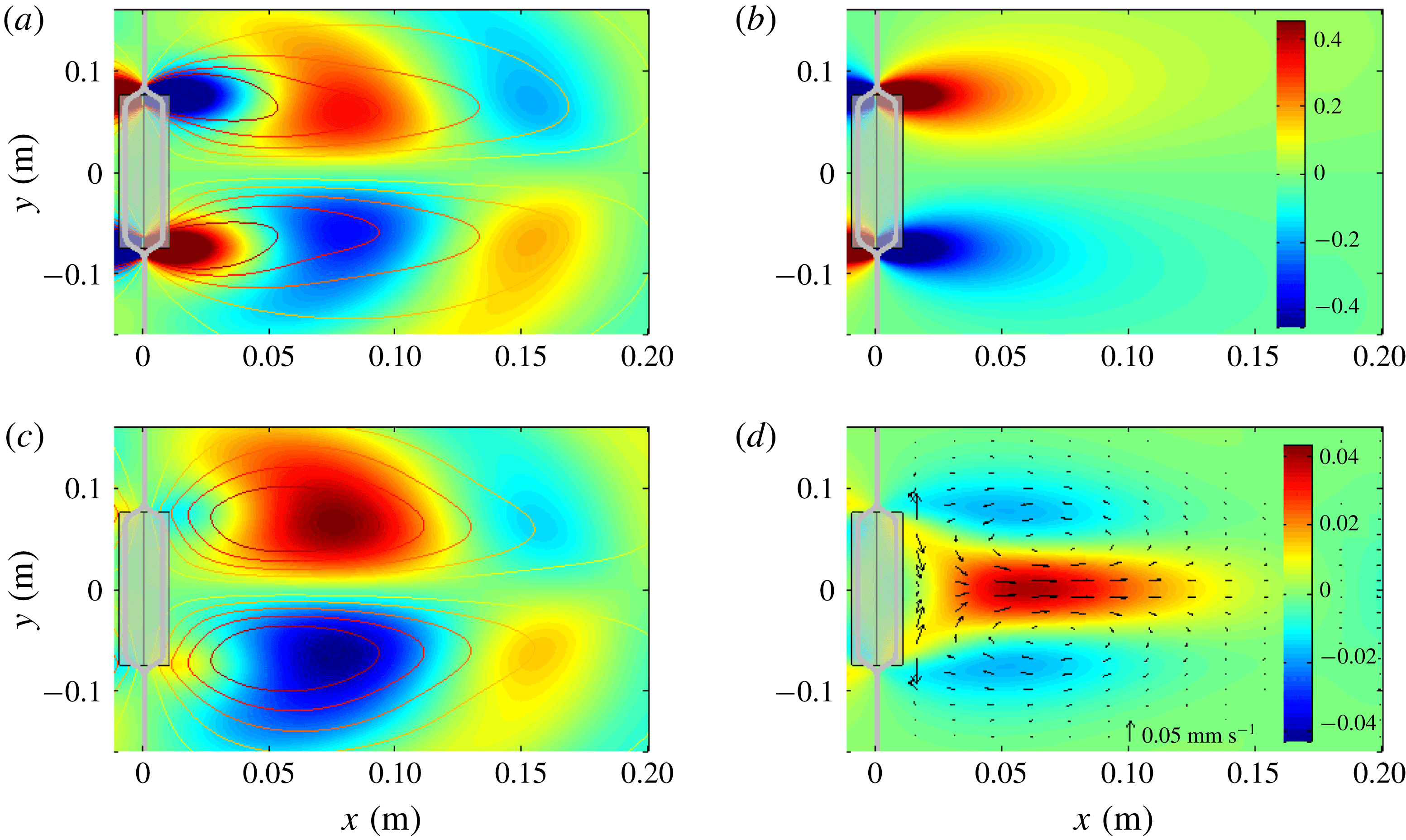Panel (d) presents the net Stokes drift in the $x$ -direction,  $\bar{u}_{S}$ , with arrows indicating the horizontal Stokes drift field,  $[\bar{u}_{S},\bar{v}_{S}]$ , possibly representing the initially observed jet that Bordes et al. (Reference Bordes, Venaille, Joubaud, Odier and Dauxois2012) refer to, as discussed in the text.

Figure 8.

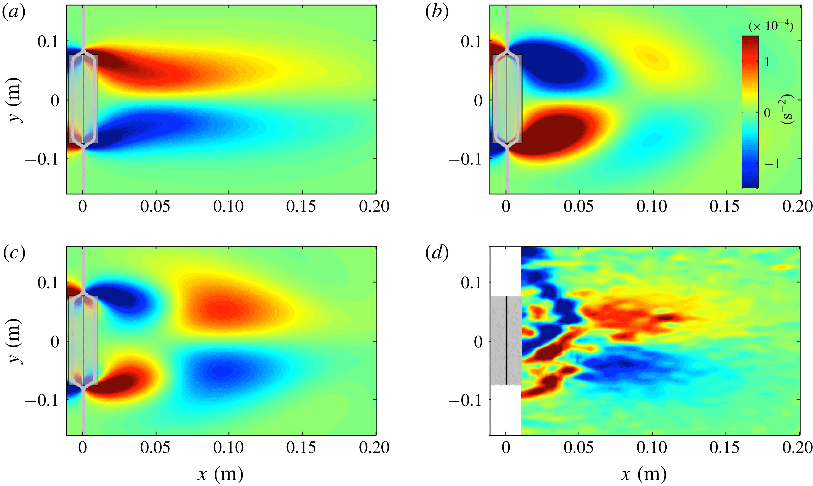
The theoretical mean vertical vorticity production associated with (a) streaming, $\bar{R}_{0}^{b}$ , (b) interaction of the vertical line vortices with the beam, $\bar{R}_{0}^{cf}$ , and (c) their combined production. The mean vertical vorticity increase, $\unicode[STIX]{x2202}_{t}\bar{\unicode[STIX]{x1D6FA}}$ , experimentally observed by Bordes et al. (Reference Bordes, Venaille, Joubaud, Odier and Dauxois2012) and presented in their figure 3(a), is reproduced in panel (d).

7 Concluding remarks

Our analysis has once again confirmed that the propagation of 3D internal gravity wave beams differs fundamentally from their 2D counterparts. In agreement with the results by Bordes et al. (Reference Bordes, Venaille, Joubaud, Odier and Dauxois2012) and Kataoka & Akylas (Reference Kataoka and Akylas2015), we find that the finite width of 3D internal gravity wave beams is essential in producing mean vertical vorticity through streaming, resulting in a strong horizontal mean flow.

Our results are primarily useful for the understanding of laboratory experiments on internal waves, or, reversely formulated, for avoiding misinterpretation of experimental results. As such, our work may contribute to correct and insightful extrapolations of experimental results to oceanic circumstances.

Importantly, we find that the vertical line vortices at the lateral edges of the wave maker contribute to the mean vertical vorticity production at leading order, and can therefore not be neglected. Moreover, this vertical vorticity production changes sign with increasing distance to the wave maker, the rate being imprinted by the horizontal beam wavelength. It is this sign change which results in the quadrupolar structure of the mean vertical vorticity production, which was also observed experimentally.

One may wonder why the quadrupolar vertical vorticity production leads to a dipolar induced mean flow (evident in figures 1(b) and 2(d) of Bordes et al. (Reference Bordes, Venaille, Joubaud, Odier and Dauxois2012)), rather than a quadrupolar induced mean flow. The answer is surprisingly simple. The stress of the wave maker on along-boundary mean flow produces a boundary layer with thickness $\sqrt{\unicode[STIX]{x1D708}t}$ (see e.g. Schlichting & Gersten Reference Schlichting and Gersten2000), reaching 1 cm thickness within four wave periods and almost 4 cm by the end of the experiment. This means that the dipole associated with the vertical line vortices eventually ends up inside the boundary layer of the vortical induced mean flow, and is thus strongly damped by wall friction. The good agreement of the simulated induced mean flow by Kataoka & Akylas (Reference Kataoka and Akylas2015) with the experiments stems from the circumstance that the near-field induced mean flow (associated with the wave–line vortex interaction and ignored in their theory) quickly reaches a state in which its energy input matches the wall-friction dissipation rate, whereas the far-field induced mean flow (forced by streaming) accumulates mean vertical vorticity throughout the entire experiment.

A standard paradigm (also known as non-acceleration theorem) widely used in fluid dynamics says that the resonantly growing induced mean flow can only arise when and where waves are (A) dissipated or (B) generated (e.g. Andrews & McIntyre Reference Andrews and McIntyre1978). In our setting, streaming belongs to the dissipative processes (A), which may occur anywhere in space, whereas the inviscid generation mechanism associated with the vertical line vortices only occurs in the vicinity of the energy source (B). The notion of ‘vicinity’ is obviously problem-dependent, ranging from a few centimetres in laboratory set-ups to possibly dozens of kilometres in oceanographic settings. Although counterexamples are known (Bühler & McIntyre Reference Bühler and McIntyre2005), this paradigm nevertheless forms a suitable conceptual classification of the two vortical mean flow generation mechanisms discussed here.

The Helmholtz decomposition has proven extremely useful in many studies on fluid dynamics (see e.g. the review by Bhatia et al. (Reference Bhatia, Norgard, Pascucci and Bremer2013)), including recent developments for internal wave data analysis (Bühler, Kuan & Tabak Reference Bühler, Kuan and Tabak2017). Once more, we find that disentangling the wave horizontal wave field with a Helmholtz decomposition into propagating internal wave ( $\unicode[STIX]{x1D719}$ ) and non-propagating oscillation ( $\unicode[STIX]{x1D6F9}$ ) is essential in determining the mean vertical vorticity production contributions. It is now a standard procedure to disentangle experimental wave field data in vertical planes into field components propagating in different vertical directions through Hilbert filtering (Mercier, Garnier & Dauxois Reference Mercier, Garnier and Dauxois2008). We propose to extend the experimental wave field decomposition procedure with a (discrete) Helmholtz decomposition applied to the horizontal velocity field in horizontal planes to disentangle wave and vortex components.

Possibly most importantly, our analysis in § 3 illustrates that an appropriate mathematical representation of the wave maker is essential in studies on mean flow generation. The numerical code by Sibgatullin & Kalugin (Reference Sibgatullin and Kalugin2016), used in several studies involving wave makers, and the numerical code employed by Grisouard et al. (Reference Grisouard, Leclair, Gostiaux and Staquet2013) and Raja (Reference Raja2018), for simulations of mean flow generation upon reflection at inclined bottoms, do not capture the vertical line vortices at the edges of the wave makers. While the absence of the vertical line vortices in simulations may be of no concern for the far field, one must be aware that the vertical line vortices are intrinsic to laboratory experiments, and may impact the nonlinear dynamics in the vicinity of the wave maker. Brouzet et al. (Reference Brouzet, Sibgatullin, Scolan, Ermanyuk and Dauxois2016) find mean flow generation in their numerical simulations, possibly related to streaming in the boundary layer at the rigid walls. A similar study by Pillet et al. (Reference Pillet, Ermanyuk, Maas, Sibgatullin and Dauxois2018) places a wave maker in a much wider tank, resulting in lateral spreading of the internal wave field. Based on our analysis, we expect mean flow generation associated with the line vortices at the edges of the wave maker in the laboratory, this being absent in the corresponding numerical simulation. The strengths of our theoretical study is that we can ‘switch’ on and off the vertical line vortices, thereby investigating whether incorporating the line vortices may be important for more complicated configurations that can be tackled only numerically.

This work also forms the basis for further research on the effect of rotation ( $f\neq 0$ ) on strong mean flow generation. Numerical simulations by Raja (Reference Raja2018), as well as recent work by Wagner & Young (Reference Wagner and Young2015) and Fan et al. (Reference Fan, Kataoka and Akylas2018), indicate mean flow generation to be strongly influenced by rotation. Using the wave maker representation derived in § 3, it is straightforward to incorporate the effect of rotation on streaming, soon to be presented in a separate paper.