2.1. Problem statement

To explore the physical mechanisms underlying the spatio-temporal organisation of the flow, we performed a systematic parametric study using a symmetric two-dimensional (2-D) planar channel of diameter $2R$ , whose walls are patterned with moving ridge-like villus structures of uniform height $H$ and width $W$ , as illustrated in figure 1. Previous three-dimensional (3-D) simulations of stationary contractions by Lim et al. (Reference Lim, de Loubens, Love, Lentle and Janssen2015), with different 3-D villus shapes, show only minor qualitative differences in the resulting flow fields.

The fluid flow is solved both in the intervillous spaces and in the main channel lumen. The villi are modelled as rigid structures. To validate this assumption, we carry out a simple order of magnitude calculation considering a single villus as a slender cantilever beam of length $L \approx 500\, \unicode{x03BC} {\textrm {m}}$ and square cross-section of width $W \approx 200\, \unicode{x03BC} {\textrm {m}}$ . The villus beam, made up of healthy intestinal extracellular matrix, is given to possess a Young’s modulus of ${\approx}2.9$ kPa (Creff, Malaquin & Besson Reference Creff, Malaquin and Besson2021). At a large chyme viscosity of $100$ mPa s, a maximum wall strain rate of ${\approx} 0.47$ s⁻¹ was computed for physiologically mapped pendular motion in the rat gut (de Loubens et al. Reference de Loubens, Lentle, Love, Hulls and Janssen2013). Using the slender beam theory, purely viscous stresses here would result in a maximum villus tip deflection of ${\lt} 0.5\, \unicode{x03BC} {\textrm {m}}$ . This is ${\lt } 0.1\,\%$ of the total villus length, validating the rigidity assumption for the villi. The rigid villi condition is further supported by two experimental studies (Lentle et al. Reference Lentle, Janssen, de Loubens, Lim, Hulls and Chambers2013; Lim et al. Reference Lim, Lentle, Janssen, Williams, de Loubens, Mansel, Chambers and Blachier2014), which demonstrate that villus motion is driven by contractions of the underlying muscularis mucosa and does not result from bending deformation under physiological fluid shear stresses. Note that in the brushtail possum, smooth muscle contractions induce wrinkling of the mucosa (Lentle et al. Reference Lentle, Janssen, de Loubens, Lim, Hulls and Chambers2013). We neglect this phenomenon in the present model, as our ongoing experiments in the rat duodenum have not shown such wrinkling, suggesting that it may be species-dependent.

The spatial coordinates along the axial and radial dimensions of the channel are given by $\boldsymbol{x} = (z, r)$ , respectively. Along $r$ , the channel is bounded by a moving wall at $r = 0$ , detailed with $N$ periodic villi and a symmetry boundary at $r = R$ . The domain is periodic along $\pm {z}$ . For the purpose of analysis, the domain is parted into two zones: the region patterned with villi where $0\leqslant r \leqslant H$ is termed the villi zone and the channel space where $H \lt r \leqslant R$ is termed the lumen zone. The villi harmonically oscillate along $z$ , in time period $T$ , around their mean axial positions, as shown in figure 1(c). The mean villi positions (orange outlines in figure 1) are equispaced by distance $P$ along $\boldsymbol{z}$ , therefore giving a periodic channel length of $L_z = \textit{NP}$ .

Each individual villus, indexed $i=1,2,\ldots, N$ , is put into axial translation by propagating contractions of the longitudinal smooth muscle cells of the small intestine (Lentle et al. Reference Lentle, de Loubens, Hulls, Janssen, Golding and Chambers2012). Consequently, the ${i}{\textrm{th}}$ villi velocity is modelled as

(2.1) \begin{equation} \boldsymbol{U}_i(t) = \omega a \sin \left ( \omega t + (i-1) \Delta \phi \right ) \hat {\boldsymbol{z}}, \end{equation}

and the ${i}{\textrm{th}}$ villi axial position is

(2.2) \begin{equation} \boldsymbol{X}_i(t) = \overline {\boldsymbol{X}}_i - a \cos \left ( \omega t + (i-1) \Delta \phi \right ) \hat {\boldsymbol{z}}, \end{equation}

where $\omega =2 \pi f$ is the circular frequency, $f=1/T$ is the oscillation frequency, $a$ is the oscillation amplitude, $t$ is the time, $\Delta \phi$ is the phase lag between adjacent villi, $\overline {\boldsymbol{X}}_i$ is the mean axial villi position and $\hat {\boldsymbol{z}}$ is the unit vector along the axial direction.

Since we model a finite number of villi, we can access only discrete values for the phase lag $\Delta \phi = 2 \pi /N$ . When $N = 1$ , $\Delta \phi = 2 \pi$ , meaning all villi are moving in-phase. This is equivalent to the case where $N$ becomes large ( $N \to \infty$ ), and $\Delta \phi \to 0$ , a situation recently studied in 3-D by Puthumana Melepattu & de Loubens (Reference Puthumana Melepattu and de Loubens2022). When $N = 2$ , $\Delta \phi = \pi$ and adjacent villi move with velocities exactly out-of-phase. In the intermediate situation, i.e. $0 \lt \Delta \phi \lt \pi$ (or $3 \leqslant N \lt \infty$ ), a propagating wave of intervillous contraction is generated along the villi wall. We term this as the pendular-wave activity. This wave travels in the $-\hat {\boldsymbol{z}}$ direction at a speed of $c=L_z/T = 2 \pi f P / \Delta \phi$ . Figure 1(d) demonstrates how contractions and relaxations along the intervillous spaces (see marked rectangular regions) travel from right to left along $-z$ . The bottom walls of the intervillous gaps are assigned instantaneous velocities that are linearly interpolated between those imposed by their bounding villi.

The fluid is assumed Newtonian, with dynamic viscosity $\mu$ and mass density $\rho$ . The intestinal fluids are generally highly heterogeneous, and the Newtonian assumption provides a well-defined baseline in the regime of low particulate volume fraction, particularly in the proximal part of the small intestine where the digesta is mixed with a large quantity of secretions (Hardacre et al. Reference Hardacre, Lentle, Yap and Monro2018). This assumption, which is also relevant in view of potential microfluidic applications, facilitates the elucidation of the underlying physical mechanisms and the comparison across studied parameters. The flow is modelled by the incompressible Navier–Stokes equations given by

(2.3) \begin{align} \boldsymbol{\nabla } \boldsymbol{\cdot }\boldsymbol{u} & = 0, \end{align}

(2.4) \begin{align} \rho \frac {\partial {\boldsymbol{u}}}{\partial {t}} + \rho {\boldsymbol{u}} \boldsymbol{\cdot }\boldsymbol{\nabla } \boldsymbol{u} & = - \boldsymbol{\nabla } p + \mu {\nabla} ^2 \boldsymbol{u}, \end{align}

where $p$ is the pressure and $\boldsymbol{u}$ the fluid velocity vector field.

2.2. Non-dimensionalisation

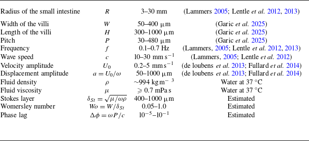
One observes that there are multiple length and time scales in the problem, as seen in table 1. We can identify time scales for four physical processes: (i) the villi oscillation time scale $t^{{\omega }} = 1 / \omega$ ; (ii) the fluid advective time scale $t^{\textit{ad}v} = W / (\omega a)$ ; (iii) the viscous time scale $t^{\mu } = W^2 \rho / \mu$ ; and (iv) the time scale imposed by the boundary travelling wave $t^{c} = W/c = W \Delta \phi / (\omega P)$ .

Table 1.

Typical values characterising villus geometry in the small intestine (mouse, rat, possum, rabbit, chicken, human, horse; see details in Garic et al. Reference Garic, Vernekar, Martín, Tanguy, de Loubens and Loverdo2025), and longitudinal motility in rat (Lentle et al. Reference Lentle, de Loubens, Hulls, Janssen, Golding and Chambers2012; de Loubens et al. Reference de Loubens, Lentle, Love, Hulls and Janssen2013), possum (Lentle et al. Reference Lentle, Janssen, de Loubens, Lim, Hulls and Chambers2013) and rabbit (Lammers Reference Lammers2005; Fullard et al. Reference Fullard, Lammers, Wake and Ferrua2014). Orders of magnitude of dimensionless parameters are estimated based on these physiological values.

Furthermore, oscillatory boundaries introduce a characteristic length scale for viscous dissipation normal to the wall, termed as the Stokes layer, $\delta _{St} = \sqrt {\mu / (\omega \rho )}$ (Schlichting Reference Schlichting1960). A priori, it is unclear which length and time scales would dominate the problem at hand. In our scenario, we have chosen the villi width $W$ as the length scale of the problem, in line with the literature (Tatsuno Reference Tatsuno1973; Kotas, Yoda & Rogers Reference Kotas, Yoda and Rogers2007; Puthumana Melepattu & de Loubens Reference Puthumana Melepattu and de Loubens2022). We make the choice for non-dimensionalisation as $\tilde {\boldsymbol{u}} = \boldsymbol{u}/(\omega a)$ , $\tilde {p} = p W/(\mu \omega a)$ , $\tilde {\boldsymbol{x}} = \boldsymbol{x}/W$ and $\tilde {t}=t \omega$ for the typical velocity, pressure, length and time, respectively, to obtain the non-dimensional momentum equation as

(2.5) \begin{equation} \frac {1}{\tilde {a}} \frac {\partial \tilde {\boldsymbol{u}}}{\partial \tilde {t}} + \tilde {\boldsymbol{u}} \boldsymbol{\cdot }\tilde {\boldsymbol{\nabla }} \tilde {\boldsymbol{u}} = - \frac {1}{\tilde {a} {\textit{Wo}}^2} \tilde {\boldsymbol{\nabla }} \tilde {p} + \frac {1}{\tilde {a} {\textit{Wo}}^2} \tilde {{\nabla} }^2 \tilde {\boldsymbol{u}}. \end{equation}

Two non-dimensional numbers emerge in (2.5), namely the Womersley number ${\textit{Wo}}=W/\delta _{St}$ (Loudon & Tordesillas Reference Loudon and Tordesillas1998) and the reduced oscillation amplitude $\tilde {a}=a/W$ . The villi motility in (2.1) can now be similarly re-written in the dimensionless form as

(2.6) \begin{equation} \tilde {\boldsymbol{U}}_i (\tilde {t}) = \sin \left ( \tilde {t} + (i-1) \Delta \phi \right ) \hat {\boldsymbol{z}}. \end{equation}

Three parameters then govern the problem, namely the boundary imposed phase lag $\Delta \phi$ , the Womersley number ${\textit{Wo}} = W/\delta _{St}$ and the reduced amplitude $\tilde {a}=a/W$ .

The geometry of villi varies both within a single species and across different species, as listed in table 1. However, the differences observed within the same region are of the same order of magnitude. Therefore, it is not relevant to study large variations in the geometric ratios. We thus fix these ratios to the typical values reported for the rat small intestine, i.e. $R/H = 5.6$ , $H/W = 2.5$ and $P/W = 1.6$ , for all simulations (Hosoyamada & Sakai Reference Hosoyamada and Sakai2005; Lentle et al. Reference Lentle, de Loubens, Hulls, Janssen, Golding and Chambers2012; Casselbrant & Helander Reference Casselbrant and Helander2022).

The longitudinal muscular activity is reported at ${\sim}0.5\,{\textrm{Hz}}$ in various species (table 1). Based on this value, the typical physiological Stokes layer thickness $\delta _{St}$ is estimated as at least 470 $\unicode{x03BC} {\textrm {m}}$ for a watery digesta. Consequently, for typical rat villi lengths of ${\sim} 500\, \unicode{x03BC} {\textrm {m}}$ , the typical physiological ${\textit{Wo}} = W/\delta _{St} \approx 0.42$ . There is no direct measurement for $\Delta \phi$ reported in the literature; we estimate it to be small, with an upper bound of 0.2. In this paper, we go beyond the limited physiological range of values of ${\textit{Wo}}$ and $\Delta \phi$ to investigate the physical mechanisms governing the flow patterns and to assess their potential for microfluidic applications. ${\textit{Wo}}$ is varied over three orders of magnitude and $\Delta \phi$ from $0$ to $\pi$ in discrete steps. Regarding the amplitude of oscillations, we restrict our study to the small-amplitude regime, with $\tilde {a} = 0.1$ and $0.2$ . This choice is motivated by previous studies on steady streaming flows, which have shown that more complex flow structures can emerge in the large-amplitude regime, even at low ${\textit{Wo}}$ (Tatsuno Reference Tatsuno1973). When ${\textit{Wo}} \ll 1$ , along with $\tilde {a}\ll 1$ , we see that (2.5) reduces to the steady Stokes equation. However, when ${\textit{Wo}} \gg 1$ , we expect an inertial flow regime, with all terms in (2.5) playing a role.

The results presented in this paper are based on a total of 128 simulations spanning the parameter space $(Wo,\, \Delta \phi ,\, \tilde {a})$ .

3.1. Two-relaxation-time lattice Boltzmann solver

We solve the incompressible Navier–Stokes equations using the lattice Boltzmann method (LBM) using the D2Q9 lattice, which discretises coordinate space in two directions and the velocity space in nine directions (He & Luo Reference He and Luo1997b ; Zhang Reference Zhang2011). The simulation code is validated for the Stokes second problem constrained to a symmetric channel to be second-order accurate with the comparisons shown in figure S1 in the supplementary material available at https://doi.org/10.1017/jfm.2025.873 and is open sourced (Vernekar et al. Reference Vernekar, Garic, de Loubens, Loverdo and Tanguy2025). One key advantage of LBM is that it solves the flow on a fixed Cartesian grid, which remains efficient even in the presence of moving boundaries. This grid-based formulation allows for straightforward parallelisation, as most operations are local. Moreover, we use the two-relaxation-time (TRT) scheme, which significantly reduces the relaxation-time-dependent error in the LBM (Ginzburg, Verhaeghe & d’Humieres Reference Ginzburg, Verhaeghe and d’Humieres2008), to accurately capture second-order flow phenomena. In the TRT-LBM, ‘distribution function’ (or ‘population’) $g$ is updated at every lattice node according to

(3.1) \begin{align} &g_i^{\ast }(t^{\ast }, \boldsymbol{x}) = g_i(t,\boldsymbol{x}) + \frac {1}{\tau ^+} \left(g^{eq+}_i(t,\boldsymbol{x}) - g^+_i(t,x)\right) + \frac {1}{\tau ^-} \left(g^{eq-}_i(t,\boldsymbol{x}) - g^-_i(t,\boldsymbol{x})\right)\!, \end{align}

(3.2) \begin{align} &g_i(t+\Delta t, \boldsymbol{x+\Delta x}) = g_i^{\ast }(t^{\ast }, \boldsymbol{x}), \end{align}

where $\boldsymbol{x}$ is the position coordinate, $t$ the time and the index $i=0,1,\ldots ,8$ indicates discrete lattice velocity directions. For the ${i}{\textrm{th}}$ direction, $\boldsymbol{x}+\boldsymbol{\Delta x} = \boldsymbol{x}+\boldsymbol{e}_i\Delta t$ , where $\boldsymbol{e}_i$ is the lattice velocity vector (Krüger et al. Reference Krüger, Kusumaatmaja, Kuzmin, Shardt, Silva and Viggen2017). Here, $\tau ^+$ and $\tau ^-$ are the two relaxation times associated with symmetric ( $^+$ ) and anti-symmetric ( $^-$ ) parts of the populations which are defined as

(3.3) \begin{equation} g^+_i = \frac {g_i + g_{\bar {i}}}{2}, \quad g^-_i = \frac {g_i - g_{\bar {i}}}{2}, \quad g^{eq+}_i = \frac {g^{eq}_i + g^{eq}_{\bar {i}}}{2}, \quad g^{eq-}_i = \frac {g^{eq}_i - g^{eq}_{\bar {i}}}{2}, \end{equation}

where the direction $\bar {i}$ is defined such that $\boldsymbol{e}_{\bar {i}} = - \boldsymbol{e}_i$ .

We use the incompressible equilibrium of He & Luo (Reference He and Luo1997a ), which is given as

(3.4) \begin{equation} g^{eq}_i (\boldsymbol{x}, t) = w_i \rho + w_i \rho _0 \left (\frac {\boldsymbol{u}\boldsymbol{\cdot }\boldsymbol{e}_i}{c_s^2} + \frac {(\boldsymbol{u}\boldsymbol{\cdot }\boldsymbol{e}_i)^2}{2 c_s^4} + \frac {\boldsymbol{u}\boldsymbol{\cdot }\boldsymbol{u}}{2 c_s^2} \right )\!, \end{equation}

where $w_0=4/9, w_{1-4}=1/9$ and $w_{5-8}=1/36$ are the lattice direction weights, and $\rho = \rho _0 + \delta \rho$ is the fluid density, taken as the sum of constant and variable parts. For the D2Q9 lattice discretisation, $c_s= \Delta x/(\Delta t \sqrt {3})$ is the so-called ‘lattice sound speed’. In simulation (or lattice) units, we take the nodal distance $\Delta x = 1$ , the time step $\Delta t = 1$ and $\rho _0=1$ . Using the incompressible equilibrium rather than the more popular compressible equilibrium is important to accurately capture the time-integrated steady streaming flow.

The macroscopic variables in the solution are recovered through

(3.5) \begin{align} \rho & = \sum _i g_i \quad \textrm{and} \quad \boldsymbol{u} = \frac {1}{\rho _0} \sum _i \boldsymbol{e}_i g_i, \end{align}

(3.6) \begin{align} p & =c_s^2 \rho \quad \textrm{and} \quad p_0=c_s^2 \rho _0, \end{align}

where $p$ gives the fluid pressure and $p_0$ is the datum pressure. Through Chapman–Enskog analysis, the kinematic viscosity is related to the relaxation time as $\nu = c_s^2 (\tau ^{+} - \Delta t/2)$ (Ginzburg et al. Reference Ginzburg, Verhaeghe and d’Humieres2008).

The LBM algorithm follows two simple steps: first, ‘collision’, where (3.1) is evaluated at some intermediate time $t^{\ast } \gt t$ , followed by ‘streaming’ (3.2), where the post-collision populations advance to their neighbouring nodes at the end of $t+\Delta t$ . This completes one time step $\Delta t$ at the end of which the macroscopic variables $\boldsymbol{u}$ and $p$ are computed from (3.5) and (3.6). These are then used to compute equilibrium distribution $g^{eq}$ from (3.4) for the next time step.

3.2. Moving boundary condition

In contrast to the LB simulations involving cilia (Hall & Clarke Reference Hall and Clarke2020), where the elongated microstructures are thinner than one lattice unit, villi have a finite thickness that spans several lattice nodes. The complex boundary in this study demands a higher-order LB scheme for treating moving boundaries to obtain an accurate solution for the instantaneous and steady streaming flows around the villi and in the lumen. It is equally important to adopt a robust ‘fresh’ node treatment alongside the scheme to ensure a stable solution and prevent degradation of accuracy. Fresh nodes are those lattice nodes that transition from inside the villi into the fluid zone as the villi boundary moves, and where $\rho$ and $\boldsymbol{u}$ need to be guessed. We therefore use a second-order accurate interpolated bounce-back scheme (IBB), alongside an iterative procedure to re-fill values for fresh fluid nodes (Ginzburg et al. Reference Ginzburg, Verhaeghe and d’Humieres2008; Chen et al. Reference Chen, Yu, Lu and Hou2014).

The IBB scheme is adapted from the family of linear interpolation (LI) schemes that are computationally local at a lattice node (Ginzburg et al. Reference Ginzburg, Silva, Marson, Chopard and Latt2023). If the boundary node on the fluid side is at $\boldsymbol{x}_F$ and the villi wall lies at $\boldsymbol{x}_W = \boldsymbol{x}_F + q \boldsymbol{e}_i$ , where $q$ is the fractional distance to the wall along direction $i$ , the unknown population along $\bar {i}$ to be streamed from the wall to node at $\boldsymbol{x}_F$ is computed as

(3.7) \begin{align} g_{\bar {i}} (\boldsymbol{x}_F, t+\Delta t) &= a_1 g^{\ast }_i (\boldsymbol{x}_F, t^{\ast }) + a_2 g^{\ast }_{\bar {i}} (\boldsymbol{x}_F, t^{\ast }) + \mathcal{A}_i + \mathcal{W}_i, \end{align}

(3.8) \begin{align} \mathcal{A}_i &= a_3 \left ( I^{\textit{FF}} g_i (\boldsymbol{x}_F, t+\Delta t) + (1-I^{\textit{FF}}) g_i (\boldsymbol{x}_F, t) \right )\!, \end{align}

(3.9) \begin{align} \mathcal{W}_i &= a_0 \frac {w_i}{c_s^2} \rho _0 \frac {\boldsymbol{u}_W(t) + \boldsymbol{u}_W(t+\Delta t)}{2} \boldsymbol{\cdot }\boldsymbol{e}_i, \\[9pt] \nonumber \end{align}

where $a_{0-3}$ are interpolation coefficients and $\boldsymbol{u}_W$ is the wall velocity. We set $I^{\textit{FF}} = 1$ when $\boldsymbol{x}_{\textit{FF}} = \boldsymbol{x}_{F} - \boldsymbol{e}_i \Delta t$ is a fluid node, whereas $I^{\textit{FF}} = 0$ when $\boldsymbol{x}_{\textit{FF}}$ is a solid node (i.e. lies within the villi).

The interpolation weights are set according to

(3.10) \begin{equation} a_0 = \frac {3}{5} \left ( \frac {4}{1+2q} \right )\!, \quad a_1 = a_0 \left ( \frac {1}{2} + q \right ) -1, \quad a_2 = 1 - \frac {1}{2} a_0, \quad a_3 = 1 - (a_1 + a_2). \end{equation}

Note that in (3.10), the prefactor for $a_0$ is set to $(3/5)$ for reasons of simulation stability and to minimising velocity oscillations due to fresh node transitions (though this prefactor value can be varied in the range $[0, 1]$ ). For all reported simulations, we take 20 lattice nodes for the width $W$ of each villi and 32 lattice nodes for the pitch $P$ .

3.3. Fresh node treatment

The process of re-initialising all $g_i$ values at the nodes that are uncovered into the fluid side (as the villi move) is called as fresh node treatment. This is a major source of error as well as of numerical velocity oscillations in our computations and, therefore, needs to be handled in a robust manner (Chen et al. Reference Chen, Yu, Lu and Hou2014; Ginzburg Reference Ginzburg2025). We adopt the local iteration refill (LIR) procedure, with slight modifications, which is highly effective at countering these shortcomings (Tao, Hu & Guo Reference Tao, Hu and Guo2016). In the LIR, we first identify groups of connected fresh nodes (at least one fresh node neighbour along $\boldsymbol{e}_i$ ) and carry out the following procedure.

1. (i) Execute local collision step for all link-wise fluid neighbour nodes identified for a fresh node group using (3.1).

2. (ii) Fresh nodes are partially re-filled by streaming-in post-collision populations from their neighbour nodes using (3.2) as $g^{\star }_i$ .

3. (iii) Fill-in the remaining unknown populations $g^{\star }_i$ using interpolated bounce-back from (3.7).

4. (iv) Compute temporary populations moments $(\rho ^{\star }, \boldsymbol{u}^{\star })$ from (3.5).

5. (v) Then, compute $g^{eq,{\star }} (\rho ^{\star }, \boldsymbol{u}^{\star })$ at the fresh nodes from (3.4).

6. (vi) Carry out local collision step for all fresh nodes using (3.1).

Steps (ii)–(vi) are repeated for 5 inner-iterations, which has been shown to give sufficiently converged values of $(\rho ^{\star }, \boldsymbol{u}^{\star })$ (Marson et al. Reference Marson, Thorimbert, Chopard, Ginzburg and Latt2021). During the inner-iterations, we update $\rho , \boldsymbol{u}$ and populations $g^{eq}, g$ only at the fresh nodes (and not at their link-wise neighbours).

3.4. Numerical convergence

The computations are initiated with the fluid at rest in the channel. As the simulation advances in time, the continuous evolution of the instantaneous flow field is obtained. At the end of every oscillation period $T$ , we compute the developing SSF, $\boldsymbol{u}^{{\textit{ss}},\bullet }$ , by numerically integrating the LBM solution over all time steps of the last competed time period. At the end of a time period, say when $t=T^{\prime }$ , this can be written as

(3.11) \begin{equation} \boldsymbol{u}^{{\textit{ss}}, \bullet } (\boldsymbol{x})|_{T^{\prime }} = \frac {\Delta t}{T} \sum _{i}^{T/\Delta t} \boldsymbol{u} (\boldsymbol{x}, T^{\prime }-T+i \Delta t). \end{equation}

This developing SSF velocity field is then compared with the developing SSF field computed at the end of the previous time period, say when $T^{\prime \prime } = T^{\prime }-T$ , using the $L2$ norm as

(3.12) \begin{equation} {E}_{L2} = \sqrt { \frac { \sum _{\boldsymbol{x}} \left ( \boldsymbol{u}^{{\textit{ss}},\bullet }(\boldsymbol{x})|_{T^{\prime \prime }} - \boldsymbol{u}^{{\textit{ss}},\bullet }(\boldsymbol{x})|_{T^{\prime }} \right )^2 }{ \sum _{\boldsymbol{x}} \left ( \boldsymbol{u}^{{\textit{ss}},\bullet }(\boldsymbol{x})|_{T^{\prime \prime }} \right )^2 }}. \end{equation}

When ${E}_{L2}$ falls below 1 %, the SSF is considered to have converged and the simulation is set to terminate after running for one additional time period, $t = T^{\prime } + T$ . During this final period, the time-periodic instantaneous velocity field $\boldsymbol{u}(\boldsymbol{x}, t)$ and the steady streaming flow $\boldsymbol{u}^{{\textit{ss}}}(\boldsymbol{x})$ are recorded.

Figure 2.

Flow induced by non-propagation oscillations of the villi over two neighbouring villi at ${\textit{Wo}}=0.5$ . Instantaneous flow at $t/T=0.3$ for (a) in-phase ( $\Delta \phi =0$ ) and (b) out-of-phase ( $\Delta \phi =\pi$ ) villi motion. The colour fields map the magnitude of instantaneous velocity ( $|{\boldsymbol{u}}|/U_0$ ). Time-averaged steady streaming flow-fields ( $\boldsymbol{u}^{\textit{ss}}$ ) for (c) in-phase ( $\Delta \phi =0$ ) and (d) out-of-phase ( $\Delta \phi =\pi$ ) villi motion. The colour fields map the magnitude of $|\boldsymbol {u}^{\textit{ss}}|/U_0$ . The width of the streamlines is proportional to the local velocity magnitude. See also figures S2–S4 in the supplementary material.

4.1. Instantaneous flow

Figure 2(a) shows the instantaneous flow-field for $\Delta \phi = 0$ , for ${\textit{Wo}}=0.5$ at a given time instance. This is the 2-D equivalent of the synchronised oscillations of an infinite array of villi recently studied in detail by Puthumana Melepattu & de Loubens (Reference Puthumana Melepattu and de Loubens2022). At low ${\textit{Wo}}$ , the flow closely follows the oscillations of the villus walls. As ${\textit{Wo}}$ increases and $\delta _{St}$ decreases, inertial effects progressively localise the flow near the villus tips and introduce a lag in the lumen (see figure S2). This results in transient recirculation zones above the villus tips.

When $\Delta \phi = \pi$ , neighbouring villi oscillate exactly out of phase, as shown in figure 2(b) for ${\textit{Wo}}=0.5$ at a given time step. This motion generates counter-rotating vortical flow in the domain. With increased ${\textit{Wo}}$ , these vortical structures localise near villi tips (similarly to $\Delta \phi =0$ cases) due to radial confinement by a decreasing $\delta _{St}$ (see figure S3).

4.2. Steady streaming flow

We compute the SSF $\boldsymbol{u}^{\textit{ss}}$ as the time-integrated mean flow, using (3.11). These are plotted for ${\textit{Wo}}=0.5$ in figures 2(c) and 2(d) for $\Delta \phi =0$ and $\Delta \phi =\pi$ , respectively. The SSF is characterised by counter-rotating vortices just above the villus tips, with amplitudes several orders of magnitude lower than the instantaneous flow velocity.

For the synchronised oscillation case $\Delta \phi =0$ , an outer region of weak unidirectional steady flow develops in the lumen (see figure S4). The strength of this flow increases with increasing ${\textit{Wo}}$ in agreement with the Rayleigh streaming theory (Tatsuno Reference Tatsuno1973; Puthumana Melepattu & de Loubens Reference Puthumana Melepattu and de Loubens2022). No such outer streaming region develops for the case $\Delta \phi =\pi$ . The key point here is that for non-propagating contractions, $\Delta \phi =0$ and  $\pi$ , irreversible SSF manifests as an inertial phenomenon and $\boldsymbol{u}^{\textit{ss}}(\boldsymbol{x}) \approx 0$ in the Stokes flow regime when ${\textit{Wo}} \ll 1$ .

5.1. Instantaneous flow

Figures 3 and 4 show the flow-fields for ${\textit{Wo}}=0.16$ and ${\textit{Wo}}=2.82$ , respectively, for two values of $\Delta \phi$ in panels (a) and (b), at a given time instance. From the figures, we notice the emergence of a boundary layer above the villi tips (dashed magenta line) that separates the flow into two distinct regions. The velocity field between the villi (grey) and this boundary is characterised by asymmetric counter-rotating vortical flows of unequal strength. These vortical flows originate in the contracting intervillous gaps and terminate in those that are expanding. We call this region the MBL and its associated height is noted as $\ell$ . Above the MBL, until the central axis of the lumen at $r=R$ , we observe near-uniform unidirectional flow moving along $+\hat {\boldsymbol{z}}$ . We term this region as the advected layer.

Curiously, the vortical structures in the mixing layer are seen to propagate along $-\hat {\boldsymbol{z}}$ , carried by the imposed propagating pendular wave along the wall, while the axial flow in the advected layer goes opposite, along $+\hat {\boldsymbol{z}}$ (see supplementary movies 1–4). For the case $\Delta \phi =\pi /4$ and ${\textit{Wo}}=0.16$ (figure 3 b), the mixing layer extends all the way up to $r=R$ and the advected layer disappears. In general, the height of the MBL increases with decreasing $\Delta \phi$ , until it reaches the channel centreline. Additionally, for a given value of $\Delta \phi$ , the MBL height shrinks with an increase in ${\textit{Wo}}$ , as can be observed when comparing figures 4 and 3. The decrease of $\ell$ with ${\textit{Wo}}$ is shown in supplementary movie 5. For example, in the aforementioned case (at $\Delta \phi =\pi /4$ ), the MBL shifts from the centreline for ${\textit{Wo}}=0.16$ to approximately half-way between the centreline and villi tips for ${\textit{Wo}}=2.82$ .

The effect of propagating wave along the villi wall is felt throughout the lumen zone, irrespective of the MBL height. Figure 5 shows the measured radial velocity $u_r$ at $r=2H$ in the lumen, in panel (a), ${\textit{Wo}}=0.5$ and in panel (b), ${\textit{Wo}}=2.82$ , at increasing time-fractions $t/T$ . Right-to-left travelling wave kinematics is clearly seen in these plots, with a decrease in wave amplitude with increased ${\textit{Wo}}$ . A similar behaviour, but with a non-zero positive mean, is also seen for the axial velocity component $u_z$ (data not shown). This behaviour of the instantaneous velocity is seen both in the mixing and the advected layer, and the wave amplitude is seen to monotonically decreases with increasing radial distance $r$ .

Although the propagating pendular wave induces a travelling wave in the lumen (figure 5), the emergence of an advected layer that axially pumps fluid in the opposite direction is an intriguing phenomenon (figures 3 and 4). This behaviour is counter-intuitive in the context of momentum transport via travelling waves and contrasts with canonical peristaltic flow theory (Jaffrin & Shapiro Reference Jaffrin and Shapiro1971), in which the wave transports the fluid in its direction of propagation.

5.2. Steady streaming flow

The axial fluid pumping effect is not limited to the advected layer, but occurs throughout the lumen including in the mixing layer. This is demonstrated by figure 6 showing the time-integrated SSF computed for increasing ${\textit{Wo}}=0.16, 1.58$ and $5.0$ . For each ${\textit{Wo}}$ , we show five panels for decreasing values of $\Delta \phi$ (column-wise). The flow is shown over two neighbour villi (at their mean axial positions) in each simulated system, where the colour-field plots the axial component $(u^{\textit{ss}}_z)$ of the SSF velocity. Note that the SSF has a periodicity of $P$ in the axial direction. The dashed line in the plots shows the approximate height of the MBL seen in the instantaneous flow-field for each case.

Figure 6.

Steady streaming flow-field ( $\boldsymbol{u}^{\textit{ss}}$ ) streamlines for $\tilde {a}=0.2$ , plotted around a pair of adjacent villi for three increasing Womersley numbers: (a) ${\textit{Wo}}=0.16$ ; (b) ${\textit{Wo}}=1.58$ ; and (c) ${\textit{Wo}}=5.0$ (row-wise). For each ${\textit{Wo}}$ , panels for five decreasing $\Delta \phi$ values (column-wise) are shown. The colour-map plots the axial component of the steady streaming flow (SSF), ${u}^{\textit{ss}}_z$ . Note that the SSF pattern shows axial periodicity over the intervillous distance $P$ , for all cases. The dashed (orange) lines in each panel show the approximate mixing layer height $\ell$ seen in the respective instantaneous flow-fields.

For ${\textit{Wo}}=0.16$ and $1.58$ , flow in the lumen is highly uniform in the $+r$ direction, except in and around the villi zone. Nearer the villi, flow becomes serpentine (along $+\hat {\boldsymbol{z}}$ ), descending down through the intervillous spaces and curving above the villi tips. We see a small SSF vortex just above the intervillous space, as this serpentine flow meets the uniform flow above. With an increase in ${\textit{Wo}}=5.0$ , the flow is no longer radially uniform in the lumen and its strength gets greatly confined nearer the villi tips, with near zero net flow near the channel centreline.

It is worth noting that the MBL height $\ell$ does not appear to leave any signature on the SSF flow field, as evidenced by the dashed lines in figure 6. We therefore cannot directly correlate the radial variations of the SSF patterns with the emergence of the MBL discussed in § 5.1.

Figure 7.

Plot of the mixing layer height $\ell$ against the Womersley number ${\textit{Wo}} = W / \delta _{St}$ , for various $\Delta \phi$ , for (a) $\tilde {a}=0.2$ and (b) $\tilde {a}=0.1$ . Note the plateauing of the curves when ${\textit{Wo}} \leqslant 1$ and their rapid decrease with increasing ${\textit{Wo}}$ when ${\textit{Wo}} \geqslant 1$ , indicating a flow regime transition. The measured mixing layer heights $\ell$ from panels (a) and (b) collapse as a double-power law when appropriately rescaled, as plotted in panel (c), delineating the two regimes. Note that in panel (c), we have not shown the data-points for $\Delta \phi = 0$ and  $\pi$ . In panel (c), at large $x$ -axis is the viscosity dominant regime, while at small $x$ -axis is the inertial regime. Contrast the scaling for $\ell$ in the inertial regime $(\propto \delta _{St}^{1/2})$ with that for the theoretical boundary layer ( $\propto \delta _{St}$ ) for an oscillating flat plate (Schlichting Reference Schlichting1960). Transition between the two regimes appears to be smooth and we visually identify (0.83,6.66) as the critical transition point in panel (c). From this critical point, we obtain the functional transition curve: $\ell ^c = 6.66 e^{-3\tilde {a}/2} W / Wo$ , which is plotted as dash-dotted (grey) lines in panels (a) and (b). These lines indicate the viscous to inertial regime transition, for all $\Delta \phi$ and $\tilde {a}$ .

6.1. Mixing boundary layer height

The MBL height $\ell$ separates the vortical flow region from a unidirectional flow region (advected layer) above it. In our simulations, the axial velocity in the advected layer is always positive, i.e. $u_z \gt 0$ . We use this fact to characterise the height of MBL, by first decomposing the instantaneous axial velocity according to its direction as

(6.1) \begin{equation} {u}^-_{z} (r,z,t) = \begin{cases} {u}_{z} & \text{if } \, {u}_{z} \lt 0,\\ 0 & \text{otherwise}, \end{cases}\quad \text{and}\quad {u}^+_{z} (r,z,t) = {u}_{z} - {u}^-_{z}, \end{equation}

and then computing the time and axial average of the negative velocity $u^-_{z}$ as

(6.2) \begin{equation} \left\langle u^{ss-}_z \right\rangle _z (r) = \frac {1}{L_z T} \int _{0}^{L_z} \int _{t}^{t+T} u^-_z (t,z,r)\, {\rm d}t \,{\rm d}z, \end{equation}

which depends only on the radial distance $r$ . We now identify the MBL height $\ell$ as the shortest radial distance measured from the villi base at which $\langle u^{ss-}_z \rangle _z (r := \ell ) = 0$ . With this definition, we obtain the MBL height $\ell$ , measured from the villi base, within which the instantaneous velocity field is characterised by significant negative axial flow $u^{-}_z (z, r, t)$ and above which the $u^{-}_z (z, r, t)$ is negligible.

We measure $\ell$ for all simulated cases and its non-dimensional value is plotted against increasing ${\textit{Wo}}$ in figure 7 for various $\Delta \phi$ , in panel (a) for $\tilde {a}=0.2$ and panel (b) for $\tilde {a}=0.1$ . We first look at the non-propagating case with $\Delta \phi =0$ (star marker) and $\Delta \phi = \pi$ (circle marker). For synchronised oscillations of the villi, $\Delta \phi =0$ , $\ell$ remains constant at the maximum radial distance of $r=R$ for small ${\textit{Wo}}$ and then sharply decreases with a slope ${\sim} \delta _{St}$ at increased ${\textit{Wo}}$ . This linear decrease of $\ell$ with increased ${\textit{Wo}}$ mimics the dynamics due to an oscillating flat plate, except at ${\textit{Wo}}=5.0$ , where structure of the villi-wall boundary causes deviations. Here, the mixing boundary layer is controlled by the Stokes layer and the effect of the villi wall can be approximated by that of an oscillating flat plate positioned at an offset to the villi-wall base. Puthumana Melepattu & de Loubens (Reference Puthumana Melepattu and de Loubens2022) have shown that the mixing layer for synchronous oscillations is entirely an inertial phenomenon and can be controlled by changing the intervillous confinement. However, when $\Delta \phi =\pi$ , we have neighbour villi that oscillate exactly out of phase and generate a mixing layer. This mixing layer extends up to the channel centreline ( $r = R$ ), without the emergence of an advected layer.

A distinct class of behaviour is seen in the MBL $(\ell )$ plots for propagating contractions, $0 \lt \Delta \phi \lt \pi$ . Here, $\ell$ plateaus to a constant value at low ${\textit{Wo}}$ , which depends solely on $\Delta \phi$ and $\tilde {a}$ . This is a departure from the classical oscillating boundary layer theory (Schlichting Reference Schlichting1960), which predicts that at low ${\textit{Wo}}$ (i.e. in the Stokes flow regime), the viscous dissipation layer should encompass the entire channel. The plateau value of $\ell$ decreases as $\Delta \phi$ increases from $\pi /5$ to $2\pi /3$ .

At high ${\textit{Wo}}$ in the inertial regime, $\ell$ decreases with a slope ${\sim} \sqrt {\delta _{St}}$ , contrasting with the linear scaling seen for $\Delta \phi =0$ . Comparing figures 7(a) and 7(b), we also see that decreasing $\tilde {a}$ causes an increase in the relative levels of the measured MBL height. At smaller $\Delta \phi$ , e.g. for $\Delta \phi =\pi /5$ (square markers), the Stokes to inertial transition of $\ell$ occurs at a smaller ${\textit{Wo}}$ , as compared with that at larger values e.g. $\Delta \phi = \pi /2$ (triangle markers). The critical transition ${\textit{Wo}}$ is smaller for larger plateau values of $\ell$ (i.e. smaller $\Delta \phi$ values). Here, for $\Delta \phi \leqslant \pi /4$ , the increasing mixing layer height is truncated by the radial confinement of the geometry. For these cases, the mixing layer extends across the entirety of the lumen at ${\textit{Wo}} \ll 1$ and the advected layer disappears.

The plots also appear to show an apparent increase of $\ell$ at high ${\textit{Wo}}=5.0$ for certain cases, namely for $(\tilde {a}=0.2, \Delta \phi =\pi /5$ ) (see supplementary movie 6), and for $(\tilde {a}=0.1, \Delta \phi =\pi /5)$ and $(\tilde {a}=0.1, \Delta \phi =\pi /4)$ (see supplementary movie 7). Upon further investigation, we find that the flow structure in these cases is unlike that observed in the rest of the simulations. Here, the vortical flow pattern emanating from the villi is altered, with the smaller counter-clockwise vortical flow assuming a distinct hourglass-like shape, while the larger clockwise vortical flow reaching the channel centre. Despite the high oscillatory inertia at ${\textit{Wo}} = 5.0$ , we have a mixing layer height that reaches the channel centre. Here, the steady streaming flow gets significantly weakened (see figure 6 c, right-most panel) and the vortical instantaneous flow dominates throughout the luminal space. This changed flow structure indicates the existence of another inertial flow transition beyond ${\textit{Wo}} \gtrsim 5$ , which would also depend on $\Delta \phi$ and $\tilde {a}$ . Here, the computed averaged MBL height ( $\ell$ ) is inconsistent due to the change in the flow structure for these cases. In this paper, we limit ourselves to ${\textit{Wo}} \leqslant 5.0$ and a well-defined $\ell$ , and therefore exclude these three points from further analysis in the present section.

The mixing layer height data show a phenomenological collapse onto a double power-law master curve, as shown in figure 7(c). Since the data for non-propagating cases ( $\Delta \phi =0$ and $\pi$ ) exhibit a different class of behaviour, it does not collapse onto the master curve and is therefore not shown. The $x$ variable for the collapse is $\delta _{St} \Delta \phi ^{2/3} / H$ and the $y$ variable is $\ell / (e^{-3\tilde {a}/2} \delta _{St})$ . Physically, the $y$ variable represents the MBL height normalised by the viscous penetration layer above the villi, after correcting for spatial attenuation associated with the oscillatory amplitude. The $x$ variable is $\propto 1/Wo$ and quantifies the relative reduction of oscillatory inertial effects, rescaled by the leading-order dependence of the MBL height on the phase lag. For large values of the $x$ variable, the flow is dominated by viscous effects, leading to the power law relation $y \propto x^{-1}$ (blue line) and, thus, $\ell \propto \Delta \phi ^{-2/3} e^{-3\tilde {a}/2}$ . Here, the mixing layer height $\ell$ is unaffected by oscillatory fluid inertia and is therefore independent of $\delta _{St}$ , identifying the parameter set that falls within the viscous dominated regime.

However, as the $x$ variable decreases, the flow transitions into the oscillatory inertial regime, with the power law relation $y \propto x^{-1/2}$ (red line). The mixing layer height now depends on ${\textit{Wo}}$ and scales as $\ell \propto \delta _{St}^{1/2} \Delta \phi ^{-1/3} e^{-3\tilde {a}/2}$ . The double power law collapse therefore shows a transition from the Stokes regime (large $x$ ) into the inertial regime (small $x$ ), with a relatively smooth transition in between. At smallest values of $x$ variable, we see that the data collapse starts to fray, suggesting that this flow structure will not sustain at highly elevated oscillatory inertia. We visually identify the critical transition point between the two regimes as $(x\approx 0.83$ , $y\approx 6.66)$ . This allows us to deduce a critical transition line expressed in terms of $\Delta \phi$ as $\ell ^c = 5.5 e^{-3\tilde {a}/2} H \Delta \phi ^{-2/3}$ , and similarly, in terms of ${\textit{Wo}}$ , as $\ell ^c = 6.66 e^{-3\tilde {a}/2} W / Wo$ . This Stokes-to-inertial critical transition line is overlaid on the unscaled $\ell /H$ data in figures 7(a) and 7(b) (grey dash-dotted line). The inertial regime is shown by the grey shaded region in all plots in figure 7.

6.2. Competing oscillatory and steady flows

We now look into the physical mechanism that leads to the appearance of distinct mixing and advected layers. Towards this end, we subtract the characteristic flow velocity $\boldsymbol{U}^{AL}$ of the advected layer from the entire flow-field. Here, the axial component of the characteristic velocity is computed as

(6.3) \begin{equation} U^{AL}_z = \frac {1}{H L_z} \int _{0}^{L_z} \int _{5H}^{R} u_z \,{\rm d}r \,{\rm d}z, \end{equation}

making sure that we integrate well above the MBL height and the radial component is set to $U^{AL}_r = 0$ .

Figure 8 shows this shifted velocity field for $\Delta \phi =\pi /2$ and ${\textit{Wo}}=0.16$ , with the height of the MBL reproduced (dashed magenta line) from figure 3(a). The shifted velocity field consists entirely of counter-rotating, semi-vortical flow structures that now extend up to the central symmetry boundary. This structure is similar to that seen when the mixing layer extends until the centreline (e.g. figure 3 b). This pattern is produced irrespective of $\Delta \phi$ in the Stokes flow regime ( ${\textit{Wo}}=0.16$ ), demonstrating that the total flow-field is simply a sum of the axial steady flow and oscillatory components.

Figure 8.

Snapshots of the purely oscillatory velocity field, visualised by subtracting a constant velocity $(U^{AL}_z, 0)$ from the instantaneous velocity $\boldsymbol{u}$ , shown for two time-fractions $t/T=0.45$ and $0.75$ , for the case $\Delta \phi = \pi /2$ , ${\textit{Wo}}=0.16$ and $\tilde {a}=0.2$ . $U^{AL}_z$ , computed from (6.3), is a measure of the irreversible axial flow velocity in the advected layer. The dashed (magenta) separation line between the mixing and advected layers is reproduced from figure 3(a).

Figure 9.

Axially averaged $(\langle \boldsymbol{\cdot }\rangle _z)$ $z$ -components of (a) the oscillatory axial velocity $\langle u^{\textit{os}}_z \rangle _z$ and (b) the steady streaming axial velocity $\langle u^{\textit{ss}}_z \rangle _z$ . These measures are computed as functions of radial distance $r/H$ , from (6.4) and (6.5) for various $\Delta \phi$ and plotted (column-wise) for three increasing Womersley numbers ${\textit{Wo}} = 0.16, 1.58$ and $5.01$ . $\tilde {a}=0.2$ . The plots demonstrate that the oscillatory flow decays exponentially in $r$ , while the steady flow (which is mostly uniform for low ${\textit{Wo}}$ ) does not.

The distinct mixing and advected layers seen in the simulations manifest due to the competition between the strength of the oscillatory flow, which generates the counter-rotating vortical structures, and the axial steady flow shown in figure 6. To understand the MBL height $\ell$ behaviour, we map the radial dependence of the steady (irreversible) and vortical flows as

(6.4) \begin{align} \big\langle u^{\textit{ss}}_z \big\rangle _{z} (r) &= \frac {1}{L_z} \int _0^{L_z} u^{\textit{ss}}_z (z,r) \,{\rm d}z \end{align}

(6.5) \begin{align} \big\langle u^{\textit{os}}_z \big\rangle _{z} (r) &= \frac {1}{2T L_z} \int _0^{L_z} \int _t^{t+T} \big|u_z (t, z,r) - u^{\textit{ss}}_z (z,r) \big|\, {\rm d}t \,{\rm d}z, \end{align}

where $\langle u^{\textit{ss}}_z \rangle _{z}$ and $\langle u^{\textit{os}}_z \rangle _{z}$ are the axially averaged steady streaming and oscillatory axial velocities. Figure 9 compares the strength of these two velocity measurements, for three increasing values of ${\textit{Wo}}$ (column-wise panels) and all $\Delta \phi$ . In figure 9(a), the oscillatory velocity $\langle u^{\textit{os}}_z \rangle _{z}$ shows an exponential decay with increasing $r/H$ , for various $\Delta \phi$ . This decay becomes more pronounced as ${\textit{Wo}}$ increases. In contrast, as seen in figure 9(b), the steady streaming $\langle u^{\textit{ss}}_z \rangle _{z}$ remains nearly constant, starting from the villi tips to the centre of the lumen at lower ${\textit{Wo}}$ , while becoming increasingly bulged just above the villi tips at higher ${\textit{Wo}}$ .

In summary, the pendular wave generates a steady axial flow. This flow is nearly uniform and depends only on $\Delta \phi$ when viscosity dominates over oscillatory inertia. The propagating contraction–expansion kinematics of the villi wall also generate axially oscillating flow, seen in the form of counter-rotating vortical structures. The strength of this oscillatory flow decays exponentially along the radial direction, with a decay rate dependent on $\Delta \phi$ . The height of the MBL is so determined by a competition between these two effects. Within the mixing layer, the oscillatory axial flow predominates, while in the advected layer, its strength falls below that of the steady streaming axial flow. Hence, in viscosity dominated cases, $\ell$ depends only on $\Delta \phi$ . As oscillatory inertia increases, a decreasing Stokes layer $\delta _{St}$ enforces a dynamic radial confinement on both the steady and oscillatory flows, causing a depletion of the steady axial flow near the channel centre, as well as a faster radial decay of the oscillatory axial flow. This in turn causes the MBL height to decrease non-trivially in the inertial regime, as a function of both ${\textit{Wo}}$ and $\Delta \phi$ , unlike that for a simple oscillating flat plate.

7.1. Scaling laws

At first glance, the irreversible axial flow pumping generated by the villi wall studied here is reminiscent of that observed in propagating waves along dense oscillating ciliary arrays (Khaderi et al. Reference Khaderi, den Toonder and Onck2011; Ding et al. Reference Ding, Nawroth, McFall-Ngai and Kanso2014; Hall & Clarke Reference Hall and Clarke2020; Ishikawa Reference Ishikawa2024). Specifically, those undergoing antiplectic metachronal waves, where the direction of wave propagation is opposite to that of net fluid pumping by the ciliary array (Ding et al. Reference Ding, Nawroth, McFall-Ngai and Kanso2014). However, individual cilia possess are deformable (an additional degree of freedom) and trace non-reciprocal effective and recovery strokes during their oscillatory cycle. This breaks the time-symmetry of the Stokes equations, and generates irreversible fluid transport. This is clearly not the case for villi, which are rigid structures (Lim et al. Reference Lim, Lentle, Janssen, Williams, de Loubens, Mansel, Chambers and Blachier2014) and undergo reversible harmonic oscillations. The non-reciprocal motion of the villi wall, resulting in steady streaming axial flow even in the Stokes flow regime, is therefore more subtle.

Building on the scallop theorem (Purcell Reference Purcell1977; Lauga Reference Lauga2011), Najafi & Golestanian (Reference Najafi and Golestanian2004) proposed a minimal model for a swimmer in Stokes flow, consisting of three spheres linked in-line, where the inter-sphere gaps undergo a cyclic non-reciprocal sequence of contraction and extension. While the individual spheres follow reciprocal trajectories, the collective behaviour of the system breaks time-symmetry and generates net propulsion in the Stokes flow regime (Najafi & Golestanian Reference Najafi and Golestanian2004, Reference Najafi and Golestanian2005). Referring to figure 1(d), it becomes clear that a similar non-reciprocal sequence is executed by any two adjacent intervillous gaps (and their bounding villi) in our system. The villi wall can thus be viewed as an array of such non-reciprocally contracting and relaxing gaps, where the additional degree of freedom is introduced via the spatial phase lag $\Delta \phi$ . This phase-lagged actuation implies that each downstream (along $+z$ ) intervillous gap reaches its minimum or maximum size slightly ahead of its upstream neighbour. This sequence is never reversed in time, ensuring non-reciprocal boundary kinematics.

The contraction–expansion of the intervillous gaps pumps fluid radially, as illustrated by the arrows in figure 1(b). The non-reciprocal motion of adjacent intervillous gaps facilitates the net transfer of some parcels of this fluid from an upstream gap to its downstream neighbour. The villi-wall boundary therefore irreversibly pumps fluid in the axial direction. Based on this mechanistic description, we develop a scaling law to describe the emergence of the oscillatory radial flow. The rate of expansion and contraction of the gap between two adjacent villi, denoted $\zeta _i$ , along the $\hat {\boldsymbol{z}}$ direction is given by

(7.1) \begin{equation} \dot {\zeta }_i = 2 a \omega \sin \left ( \frac {\Delta \phi }{2} \right ) \cos \left ( \omega t + \frac {\Delta \phi }{2} (2i-1) \right )\!. \end{equation}

Integrating this equation allows us to scale the peak oscillatory radial flux per intervillous gap, denoted $Q_r^{os,max }$ (see Appendix A.1 for details), which leads to

(7.2) \begin{equation} Q_r^{os,max } = \frac {2 a \omega H}{\pi } \sin \left (\frac {\Delta \phi }{2}\right )\!. \end{equation}

Along the axial direction, the fluid trapped in the intervillous gaps undergoes non-reciprocal motion. Taking into account the coupled effect of the gap size and the fluid velocity within the gap, we get the direction and magnitude for the steady streaming axial flux averaged over the domain length $L_z$ (see Appendix A.2). The flux within the villi zone, denoted $Q^{{\textit{ss}},v}_z$ , and that within the lumen zone, denoted $Q^{{\textit{ss}},l}_z$ , are scaled as

(7.3) \begin{equation} Q^{ss,v}_z = \frac {a^2 \omega H}{2 P} \sin \left ( \Delta \phi \right ) \quad \text{and} \quad Q^{ss,l}_z = \frac {a^2 \omega (R-H)}{2 P} \sin \left ( \Delta \phi \right )\!. \end{equation}

7.2. Axial pumping

To confirm our mechanistic scaling arguments, we numerically measure the irreversible axial flux, $Q^{{\textit{ss}}}_z$ , separately in the villi zone ( $0 \leqslant r \leqslant H$ ) and in the lumen zone ( $H \lt r \leqslant R$ ) averaged over the channel length $L_z$ as

(7.4) \begin{equation} Q^{ss,v}_z = \frac {1}{L_z} \int _{0}^{H} \int _0^{L_z} u^{\textit{ss}}_z (z,r) \,{\rm d}z\, {\rm d}r \end{equation}

and

(7.5) \begin{equation} Q^{ss,l}_z = \frac {1}{L_z} \int _{H}^{R} \int _0^{L_z} u^{\textit{ss}}_z (z,r) \,{\rm d}z\, {\rm d}r. \end{equation}

Figure 10.

Axial steady-streaming fluxes integrated over (a) the villi zone $Q_z^{ss,v}$ and (b) over the lumen zone $Q_z^{ss,l}$ , plotted against the phase lag $\Delta \phi$ , for increasing ${\textit{Wo}}$ . Flux quantities are defined as averages taken over the channel length $L_z$ . Filled markers (coloured) plot simulations with $\tilde {a}=0.2$ and empty markers (black) with $\tilde {a}=0.1$ . In both plots, the solid (red) curve is from (7.3) and derived from geometric considerations detailed in Appendix A.2. Note that in panel (b), $Q_z^{ss,l}$ shows non-monotonicity with increasing ${\textit{Wo}}$ , with the maximum irreversible steady flux occurring when ${\textit{Wo}} \approx 2.82$ .

Figures 10(a) and 10(b) show the domain averaged axial steady streaming fluxes in the villi and lumen zones, respectively, for various ${\textit{Wo}}$ . For the irreversible SSF flux in figure 10(a), we see a remarkable data collapse on the scaling equation (7.3) (solid red curve). Here, the data begin to show deviations due to increasing inertial effects only for high ${\textit{Wo}}=5.0$ for $\tilde {a}=0.1$ . The measured data for $Q^{ss, v}_z$ show minimal dependence on ${\textit{Wo}}$ , indicating that the flow in the villi zone remains well approximated by the Stokes regime, even at higher ${\textit{Wo}}$ . This behaviour arises from the significant geometric confinement of the flow within the intervillous gaps, characterised by a small $(P-W)/H$ .

The irreversible luminal flux is plotted in figure 10(b), rescaled appropriately by $\tilde {a} U_0 (R-H)$ , as a function of $\Delta \phi$ . In the viscous-dominated flow regime at low ${\textit{Wo}} \ll 1$ , the steady-state axial flux data, $Q^{ss, l}_z$ , collapse onto the same functional form (solid red curve) given by (7.3). The data points here for ${\textit{Wo}} \leqslant 0.28$ fall slightly below the scaling equation (solid line). Thus, in the Stokes flow regime, we can approximate the total steady streaming axial flux across any height $h$ of the channel as $Q^{\textit{ss}}_z = Q^{ss, v}_z + Q^{ss, l}_z \approx (W h \sin ( \Delta \phi ) ) / (2PH )$ .

However, with an increase in oscillatory inertia, the flux data no longer show a functional collapse. The flux here shows a non-monotonic behaviour with increasing ${\textit{Wo}}$ in figure 10(b). Note that $Q^{ss, l}_z$ at ${\textit{Wo}}=5.0$ is lower that that at ${\textit{Wo}}=2.82$ , for all $\Delta \phi$ . Although increasing ${\textit{Wo}}$ increases the axial velocity of the fluid in the lumen, the increased inertia also limits the radial height to pump this fluid due to dynamic radial confinement of the flow near the villi tips (see figure 6). The flux therefore reaches a maximum at ${\textit{Wo}} \approx 2.8$ and falls beyond ${\textit{Wo}} \gt 2.82$ .

Figure 11.

(a) Oscillatory radial flux $Q^{\textit{os}}_r$ per intervillous gap evaluated from (7.6) plotted (on $x$ -axis) against radial distance $r/H$ (on $y$ -axis) for $\tilde {a}=0.2$ and three different $\Delta \phi =\pi$ , $\pi /3$ and $\pi /5$ . For each $\Delta \phi$ , curves for four increasing Womersley numbers ${\textit{Wo}}=0.16$ (solid), $0.28$ (dotted), $0.5$ (dashed) and $5.0$ (dash-dotted) are shown. Note that radial flux curves at low ${\textit{Wo}}$ (for ${\textit{Wo}}=0.16$ and $0.28$ ) coincide exactly. Minor deviations from these coincident curves are seen with the onset of oscillatory fluid inertia, when ${\textit{Wo}}=0.5$ , and large deviations are seen at increased oscillatory inertia for ${\textit{Wo}}=5.0$ . (b) Peak value of radial oscillatory flux ( $Q_r^{os,max }$ ) per intervillous gap plotted against the phase lag $\Delta \phi$ , for increasing ${\textit{Wo}}$ . Filled markers (coloured) are for $\tilde {a}=0.2$ and the empty markers (black) for $\tilde {a}=0.1$ . The peak flux data-points collapse solely as a function of $\Delta \phi$ , when appropriately rescaled. The simple scaling function is shown with a dashed (green) line.

7.3. Radial pumping

The radial pumping of fluid in the channel cannot lead to an irreversible radial flow due to the confining symmetric top and bottom channel walls. Instead, all of the radially pumped fluid recirculates, forming counter-rotating semi-vortical flow structures, as seen in figures 3 and 4.

Radial pumping is quantified using radial oscillatory flux. Due to radial flow confinement, mass conservation ensures that a simple integration of the velocity field along the $z$ -axis yields zero net flux. We therefore define the oscillatory radial flux per intervillous gap as

(7.6) \begin{equation} Q^{\textit{os}}_r (r) = \frac {1}{2 \textit{TN}} \int _{0}^{L_z} \int _{t}^{t+T} \left|u_r (t,z,r) - u^{\textit{ss}}_r (z,r)\right| \,{\rm d}t \,{\rm d}z . \end{equation}

Here, $N = 2 \pi / \Delta \phi$ is the number of intervillous gaps along axial periodic length $L_z = \textit{NP}$ . Subtracting $u^{\textit{ss}}_r (z,r)$ from the instantaneous velocity ensures that we capture the periodically oscillating component of the flux. Unlike in the axial case, the radial flux per intervillous gap, $Q^{\textit{os}}_r$ , is defined to retain its radial dependence and to have equal magnitude in $\pm r$ directions.

Figure 11(a) shows the non-dimensional oscillatory radial flux $Q^{\textit{os}}_r (r)$ on the $x$ -axis, as a function of the radial distance along the $y$ -axis, for three values of $\Delta \phi =\pi$ , $\pi /3$ and $\pi /5$ , at $\tilde {a}=0.2$ . The flux curves are plotted for four increasing values of ${\textit{Wo}}=0.16$ (solid), $0.28$ (dotted), $0.5$ (dashed) and $5.0$ (dash-dotted). The radial flux rises to a peak value just outside the villi tips and then falls to zero at large $r$ for all cases. Unsurprisingly, we observe that the maximum radial flux is obtained for $\Delta \phi = \pi$ , corresponding to the case where the intervillous spaces experience the largest strain for a given villus displacement  $a$ . As $\Delta \phi$ decreases, the peak radial flux value also decreases. Moreover, the radial distance over which the flux decays to zero increases with decreasing $\Delta \phi$ ; the flux decays most rapidly for $\Delta \phi = \pi$ and most gradually for $\Delta \phi = \pi /5$ . This is consistent with the behaviour of the mixing layer height $\ell$ with decreasing $\Delta \phi$ .

In the lumen zone, when ${\textit{Wo}} \ll 1$ (i.e. ${\textit{Wo}}=0.16$ and $0.28$ ), the flux curves are coincidental for all $\Delta \phi$ . This overlap demonstrates that in the absence of fluid inertia, the $Q_r^{\textit{os}}$ and its radial dependence are solely controlled by the geometric motion of the villi wall, set by the phase lag $(\Delta \phi )$ . As ${\textit{Wo}}$ increases ( ${\textit{Wo}} \approx 0.5$ ), slight deviations away from the coincidental curves appear along $r$ , indicating an onset of inertial effects. In the oscillatory inertia dominated regime ( ${\textit{Wo}}=5.0$ ), $Q_r^{\textit{os}}$ curves decay much faster to zero along $+r$ in the lumen. This again is a consequence of decreasing $\delta _{St}$ , and the radial flux in the lumen is now a function of both $\Delta \phi$ and ${\textit{Wo}}$ . However, in the villi zone, the radial flux profiles are governed solely by the phase lag $\Delta \phi$ and these always overlap irrespective of ${\textit{Wo}}$ . Thus, similar to the axial flux, the oscillatory radial flux in the villi zone remains unaffected by oscillatory fluid inertia due to greater geometric flow confinement.

The peak value of oscillatory radial flux along $r$ is identified as $Q_z^{\textit{os}, \textit{max}} (r^{\textit{max}}) = \max (Q_z^{\textit{os}}(r))$ . Figure 11(b) plots the rescaled oscillatory radial flux as a function of $\Delta \phi$ , for increasing ${\textit{Wo}}$ . Here, we see a remarkable data collapse onto the scaling form given by (7.2) (dashed green line), for all ${\textit{Wo}}$ and $\tilde {a}$ . Minor deviations are seen for $\Delta \phi =0$ , where the flux does not remain identically zero for increasing ${\textit{Wo}}$ . When $\Delta \phi =0$ , the radial oscillatory flux is generated solely through an inertial mechanism and increases linearly with ${\textit{Wo}}$ (figure not shown). The peak radial oscillatory flux generated by this inertial mechanism ( $\Delta \phi =0$ ) is completely negligible when compared with that generated due to intervillous contractions ( $\pi /5 \leqslant \Delta \phi \leqslant \pi$ ), by at least an order of magnitude, for all  ${\textit{Wo}}$ . The peak oscillatory radial flux therefore remains unaffected by fluid inertia $(\textit{Wo})$ for $\Delta \phi \gt 0$ .