1 Introduction
Rigid rod-like particles are known to significantly strengthen the viscoelastic properties of composite materials (Christensen Reference Christensen1991). Fibre-reinforced composites have numerous industrial applications ranging from concretes to reinforced plastics broadly used in the automobile and aerospace industries. Among different types of rod-like particles, carbon nanotubes (CNTs) have various advantages related to their relatively small size, high rigidity and extremely high aspect ratio, allowing a strong enhancement of the elastic moduli of composites (Allaoui et al. Reference Allaoui, Bai, Cheng and Bai2002). However, particle aggregation under colloidal interactions lowers their effective aspect ratio and can induce thixotropic effects (Rahatekar et al. Reference Rahatekar, Koziol, Butler, Elliott, Shaffer, Mackley and Windle2006; Khalkhal, Carreau & Ausias Reference Khalkhal, Carreau and Ausias2011). Chemical treatment improves the CNT dispersion state; however, it does not completely prevent adhesive contacts between nanotubes because, being dispersed in a Newtonian solvent, CNT suspensions still show a shear-thinning behaviour (Song & Youn Reference Song and Youn2005; Fan & Advani Reference Fan and Advani2007). Therefore, a clearer understanding of the role of colloidal interactions between nanotubes is extremely important for the proper design of CNT composites.
While hydrodynamic interactions in fibre suspensions have received a great deal of attention during recent decades (see the reviews by Larson (Reference Larson1999), Petrie (Reference Petrie1999) and Férec & Ausias (Reference Férec, Ausias, Chinesta and Ausias2015)), colloidal and contact interactions have received less attention. Shear-thinning behaviour related to non-hydrodynamic interactions has been observed experimentally for suspensions composed of different types of fibres, like ceramic (Bergström Reference Bergström1998), polyamide (Mongruel & Cloitre Reference Mongruel and Cloitre1999; Chaouche & Koch Reference Chaouche and Koch2001), wollastonite (Mueller, Llewellin & Mader Reference Mueller, Llewellin and Mader2010), nontronite clay (Michot et al.
Reference Michot, Baravian, Bihannic, Maddi, Moyne, Duval, Levitz and Davidson2008), colloidal haematite (Solomon & Boger Reference Solomon and Boger1998) and multiwall CNT (Khalkhal et al.
Reference Khalkhal, Carreau and Ausias2011). Some colloidal suspensions experience strong flocculation (Wierenga et al.
Reference Wierenga, Philipse, Lekkerkerker and Boger1998; Wolf et al.
Reference Wolf, White, Melrose and Frith2007), resulting in a yield stress. In particular, Saarinen et al. (Reference Saarinen, Haavisto, Sorvari, Salmela and Seppälä2014) carefully studied the flows and the microstructure of microfibrillated cellulose suspensions near the yield point using optical coherence tomography coupled with cylindrical Couette rheometry. They revealed a strongly flocculated state of the suspension depending on the ionic strength and the shear rate, and leading to heterogeneous flows with pronounced wall slip. Yield behaviour has also been observed for non-Brownian pulp suspensions (Bennington, Kerekes & Grace Reference Bennington, Kerekes and Grace1990; Cui & Grace Reference Cui and Grace2007), and is conventionally explained in terms of the combination between fibre flexibility and inter-fibre friction. Chaouche & Koch (Reference Chaouche and Koch2001) measured the adhesive force acting between two nylon fibres of diameter ranging between 14 and
 $28~\unicode[STIX]{x03BC}\text{m}$
and found values ranging between
 $10^{-8}$
and
 $10^{-6}~\text{N}$
. To the best of our knowledge, this is the single work quantifying the colloidal forces in non-Brownian fibre suspensions and revealing the importance of these forces to the shear-thinning behaviour.
Theoretical modelling of non-Newtonian effects in fibre suspensions mostly concerns flexible fibres, whose shear-thinning behaviour is governed by the ratio of the fibre elastic modulus to the applied shear stress, and the yield stress appears as a result of the solid friction between the packed fibres (Bennington et al. Reference Bennington, Kerekes and Grace1990; Toll & Månson Reference Toll and Månson1994; Servais, Månson & Toll Reference Servais, Månson and Toll1999). In a series of papers, Klingenberg and co-workers reproduced the rheology of flexible fibre suspensions by particle-level numerical simulations (see, for instance, Schmid & Klingenberg Reference Schmid and Klingenberg2000; Switzer & Klingenberg Reference Switzer and Klingenberg2004). In addition to the solid friction, they included an attractive force between fibres. A phenomenological expression was proposed for this force: it was supposed to be exponentially decaying with the separation between fibres, linear in shear rate and independent of the mutual orientation of fibres. The authors concluded on a weak effect of this force on the suspension rheology, and maintained the interplay between the solid friction and the fibre entanglement as the main mechanism governing the non-Newtonian behaviour.
However, the abovementioned scenario cannot explain shear-thinning effects in suspensions of rigid fibres dispersed in a Newtonian solvent (Bergström Reference Bergström1998; Mongruel & Cloitre Reference Mongruel and Cloitre1999; Chaouche & Koch Reference Chaouche and Koch2001). The theoretical modelling of these effects has started quite recently. Natale et al. (Reference Natale, Heuzey, Carreau, Ausias and Férec2014) extended the models of Djalili-Moghaddam & Toll (Reference Djalili-Moghaddam and Toll2005) and Férec et al. (Reference Férec, Ausias, Heuzey and Carreau2009) to non-Newtonian lubrication contacts between fibres. They mimicked the resultant hydrodynamic and non-hydrodynamic interactions between fibres by a power-law lubrication law with shear-thinning index and consistency taken as adjustable parameters. The interaction force was weighed by the contact probability and was taken into account in the stress tensor of the suspension. When the shear-thinning index is set to 0, the interaction force between fibres becomes independent of the shear rate and leads to the yield stress in the fibre suspension (Férec, Perrot & Ausias Reference Férec, Perrot and Ausias2015). Another approach, elaborated by Ma et al. (Reference Ma, Chinesta, Ammar and Mackley2008), consists of considering a series of fibre populations having different degrees of aggregation characterized by phenomenological aggregation and destruction times. The probability density of finding a fibre in a given population with a prescribed orientation was found by a solution of the properly formulated Fokker–Planck equation, while the stress tensor was calculated by averaging over all populations and orientations. Both models gave a satisfactory correspondence with experiments, reproducing a strong shear-thinning behaviour of CNT suspensions. However, the models remain mainly phenomenological, without consideration of the adhesive interaction potential. The first model captures the shear thinning by a manually introduced power-law exponent of the nonlinear lubrication law. The second model makes use of a phenomenological rotary diffusivity of particles belonging to each population. As a consequence, the model predicts progressive particle alignment and a viscosity decrease with growing Péclet number. A more detailed study of the dynamics of aggregates composed of fibres has recently been carried out by Abisset-Chavanne et al. (Reference Abisset-Chavanne, Mezher, Le Corre, Ammar and Chinesta2013, Reference Abisset-Chavanne, Chinesta, Ferec, Ausias and Keunings2015). However, the colloidal forces have still not been taken into consideration, and the effect of the aggregates on the suspension rheology is not reported.
Since the role of the adhesive contacts on the rheology of rigid fibre suspensions remains poorly understood, we decided to construct a theoretical model considering the micromechanics of the fibre–fibre contacts with colloidal van der Waals and electrostatic interactions. The basic idea consists in calculation of the resulting colloidal force between two contacting fibres, weighing this force by the probability of interparticle contact and introducing the appropriate terms into the equation of motion and the stress tensor. In theory, the shear-thinning behaviour is not necessarily connected to particle aggregation. Non-hydrodynamic interparticle forces (scaling nonlinearly with the shear rate) will inevitably lead to nonlinear shear stress versus shear rate dependence even if the particles still remain perfectly dispersed. Clearly, the van der Waals interactions promote aggregation, which is expected to strongly affect the stress level and the orientation state of the fibres. However, it is important to inspect both of these effects separately in order to gain a clearer insight into the physics behind them. Therefore, in this work we focus only on the effect of the colloidal interactions on the fibre orientation and the suspension stress without considering aggregation. We consider only the case of overall attractive interaction, i.e. van der Waals attraction is supposed to dominate over electrostatic repulsion.
In § 2, we present our theoretical model. In § 3, we compare our model with the experimental results of Natale et al. (Reference Natale, Heuzey, Carreau, Ausias and Férec2014) and Rahatekar et al. (Reference Rahatekar, Koziol, Kline, Hobbie, Gilman and Windle2009) on the shear viscosity and the first normal stress difference of CNT suspensions. Finally, conclusions and perspectives are outlined in § 4.
2 Theory
Under shear flow, the fibres enter into close contact with their neighbours, and strong short-range forces may appear. First, in § 2.1, we will present the main assumptions of the model, then, in § 2.2, we will find the expressions for the interaction forces between fibres. In § 2.3, we will integrate these forces over the contact probability and obtain the mean interaction force. The equation of angular motion of fibres will be introduced in § 2.4. In § 2.5, we will find the fibre orientation distribution, and finally, in § 2.6, we will proceed to the calculation of the shear and normal stresses.
2.1 Main assumptions
Let us consider a steady-state simple shear flow of a suspension of perfectly rigid fibres dispersed in a Newtonian solvent of viscosity
 $\unicode[STIX]{x1D702}_{0}$
. The flow is characterized by a shear rate
 $\dot{\unicode[STIX]{x1D6FE}}$
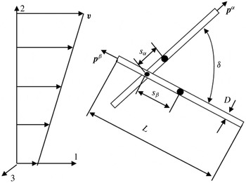
. The Cartesian coordinate frame is chosen in such a way that the axes 1, 2 and 3 correspond to the flow, velocity gradient and vorticity directions respectively, as depicted in figure 1.
Sketch of the contact between two fibres. Here,
 $v$
is the suspension velocity,
 $D$
and
 $L$
are the fibre diameter and length respectively,
 $s_{\unicode[STIX]{x1D6FC}}$
and
 $s_{\unicode[STIX]{x1D6FD}}$
are the distances between the contact point and the centre of mass of both fibres,
 $\boldsymbol{p}^{\unicode[STIX]{x1D6FC}}$
and
 $\boldsymbol{p}^{\unicode[STIX]{x1D6FD}}$
are the unit vectors describing the fibre orientation, and
 $\unicode[STIX]{x1D6FF}$
is the angle between fibres.

To get a qualitative picture of the effect of colloidal forces on the rheology of fibre suspensions, we will discard some secondary details of the experimental system and introduce the following assumptions.
(1) According to characterizations performed by Khalkhal et al. (Reference Khalkhal, Carreau and Ausias2011), the CNT particles show some distribution of their length and diameter. However, for the sake of simplicity, we shall consider the fibres to be monodisperse, thus all having the same length
 $L$
, the same diameter
 $D$
and the same aspect ratio
 $r=L/D$
. For definiteness, the average values
 $D\approx 16~\text{nm}$
of the fibre diameter and
 $r\approx 160$
of the aspect ratio will be used.
(2) The relative importance of the Brownian motion with respect to hydrodynamic interactions is described by the Péclet number (Larson Reference Larson1999):
 $Pe\approx \unicode[STIX]{x03C0}\unicode[STIX]{x1D702}_{0}L^{3}\dot{\unicode[STIX]{x1D6FE}}/[3k_{B}T(\ln r-0.8)]$
, where
 $\unicode[STIX]{x1D702}_{0}=12.3~\text{Pa}~\text{s}$
is the suspending fluid viscosity,
 $k_{B}\approx 1.38\times 10^{-23}~\text{J}~\text{K}^{-1}$
is the Boltzmann constant and
 $T\approx 300~\text{K}$
is the absolute temperature. In the range of shear rates,
 $10^{-2}\leqslant \dot{\unicode[STIX]{x1D6FE}}\leqslant 10^{2}~\text{s}^{-1}$
, used in the experiments of Natale et al. (Reference Natale, Heuzey, Carreau, Ausias and Férec2014), the Péclet number varies in the range
 $13\leqslant Pe\leqslant 1.3\times 10^{5}$
. Such high values of the Péclet number allow us to consider the CNTs as non-Brownian fibres.
(3) According to estimations of Khalkhal et al. (Reference Khalkhal, Carreau and Ausias2011) (who characterized the CNTs used in the experiments of Natale et al. (Reference Natale, Heuzey, Carreau, Ausias and Férec2014)), the CNTs are expected to be very rigid to bending within the range of the applied shear stresses. However, electron microscopy reveals some bending of fibres probably because of some local defects. The effect of such defects on the CNT orientation state under flow has recently been studied by Natale et al. (Reference Natale, Reddy, Ausias, Férec, Heuzey and Carreau2015). Keeping in mind the possible importance of CNT structural defects on the suspension rheology, we prefer to focus on the effect of colloidal interactions. Thus, at the first approximation, we consider the fibres to be perfectly rigid and straight.
(4) We consider both van der Waals attraction and electrostatic repulsion between fibres through the Derjaguin–Landau–Verwey–Overbeek (DLVO) theory adapted to rod-like particles. The electrostatic repulsion is considered at either the limit of a weak electrostatic potential
 $\unicode[STIX]{x1D6F9}$
on the fibre surface (
 $e\unicode[STIX]{x1D6F9}\ll k_{B}T$
, with
 $e$
the elementary charge) or the thin electric double layer limit (
 $\unicode[STIX]{x1D705}^{-1}\ll D$
, with
 $\unicode[STIX]{x1D705}^{-1}$
the Debye length). In these conditions, verified for non-stabilized CNT/epoxy composites, the electric double layer does not significantly increase the effective hydrodynamic diameter of fibres and, consequently, does not lead to strong excluded volume effects occurring in strongly repulsive colloids. The resulting colloidal interaction is attractive and is expected to lead to small separations,
 $h\ll D$
, between fibres at contact points, as will be proved in § 3.3.
(5) According to the work of Petrich & Koch (Reference Petrich and Koch1998), at small separations
 $h$
, the energy dissipation within the inter-fibre gaps is governed by both a hydrodynamic lubrication and a tangential solid-like friction. The latter is described by the classical Amontons–Coulomb friction law
 $$\begin{eqnarray}F_{fr}=\unicode[STIX]{x1D707}F_{\bot },\end{eqnarray}$$
where
 $F_{\bot }$
is the normal component of the resulting attractive force between particles and
 $\unicode[STIX]{x1D707}$
is the friction coefficient.
(6) We suppose only sliding contacts between particles, i.e. the fibres do not stick to each other but always slide over each other at all contact points. The sliding contacts are expected to prevent the particles from aggregation, and we neglect any possible aggregation. This assumption implies an affine translational motion of fibres, as we shall prove in § 2.3. The present hypothesis will be further discussed in §§ 2.2 and 4.
(7) The interactions between fibres and walls are neglected. This assumption should hold relatively well for the high ratio of the rheometer gap to the CNT length. To perform their experiments, Natale et al. (Reference Natale, Heuzey, Carreau, Ausias and Férec2014) used a cone-and-plate flow geometry, for which the gap at the centre of the cone was found to be 25 times larger than the longest CNT.
2.2 Interparticle forces
A sketch of the mutual position of two contacting fibres (marked as
 $\unicode[STIX]{x1D6FC}$
and
 $\unicode[STIX]{x1D6FD}$
) is shown in figure 1. The orientation of both fibres is described by unit vectors
 $\boldsymbol{p}^{\unicode[STIX]{x1D6FC}}$
and
 $\boldsymbol{p}^{\unicode[STIX]{x1D6FD}}$
, while the distance between the contact point and the centre of mass of each fibre is denoted by
 $s_{\unicode[STIX]{x1D6FC}}$
and
 $s_{\unicode[STIX]{x1D6FD}}$
. According to assumptions (4) and (5), the following short-range forces act between the contacting fibres: a lubrication force
 $\boldsymbol{F}_{lub}$
, an attractive van der Waals force
 $\boldsymbol{F}_{vdW}$
, a repulsive electrostatic force
 $\boldsymbol{F}_{el}$
and a tangential friction force
 $\boldsymbol{F}_{fr}$
. It can be shown that the normal component of the van der Waals and electrostatic forces generates only the odd moments of the orientation distribution function (
 $\langle \boldsymbol{p}\rangle ,\langle \boldsymbol{p}\boldsymbol{p}\boldsymbol{p}\rangle ,\ldots$
) in the stress tensor and in the equation of fibre rotation. Since these moments are zero because of symmetry reasons, the normal component of
 $\boldsymbol{F}_{vdW}$
and
 $\boldsymbol{F}_{el}$
does not give any contribution to the stress or the orientation state, of course, only under assumption (6) of perfect sliding without aggregation. Analysis shows that the tangential component of
 $\boldsymbol{F}_{vdW}$
and
 $\boldsymbol{F}_{el}$
appears to be negligible relative to the friction force
 $\boldsymbol{F}_{fr}$
even at low friction coefficients. Therefore, only the lubrication and solid friction forces will give leading-order contributions to the suspension stress.
The lubrication force may depend not only on the separation between fibre surfaces but also on microscopic details of the lubricated contacts, such as surface roughness and possible deformation of the contact area. Férec et al. (Reference Férec, Ausias, Heuzey and Carreau2009) have proposed a simple scaling
 $\boldsymbol{F}_{lub}\propto \unicode[STIX]{x1D702}_{0}D\boldsymbol{u}$
discarding these details, with
 $\boldsymbol{u}$
being the relative velocity of the approach of two fibres. This scaling neglects the effect of the mutual orientation of fibres. Intuitively, when the fibres get more aligned with respect to each other, the contact area increases inversely proportionally to the sine of the angle
 $\unicode[STIX]{x1D6FF}$
between fibres (figure 1). The lubrication force is roughly proportional to the contact area and is expected to be inversely proportional to
 $\sin \unicode[STIX]{x1D6FF}=|\boldsymbol{p}^{\unicode[STIX]{x1D6FC}}\times \boldsymbol{p}^{\unicode[STIX]{x1D6FD}}|$
, similarly to the case of the classical lubrication between two perfectly smooth cylinders without elastic deformations (Yamane, Kaneda & Doi Reference Yamane, Kaneda and Doi1994). Thus, the expression for the lubrication force reads
 $$\begin{eqnarray}\boldsymbol{F}_{lub}=\frac{k\unicode[STIX]{x1D702}_{0}D\boldsymbol{u}}{|\boldsymbol{p}^{\unicode[STIX]{x1D6FC}}\times \boldsymbol{p}^{\unicode[STIX]{x1D6FD}}|},\end{eqnarray}$$
where
 $k$
is a dimensionless constant depending on the microscopic details of the lubricated contact. This constant is taken as a free parameter of the model. According to assumption (5), the solid friction force (2.1) can be written in the following vector form:
 $$\begin{eqnarray}\boldsymbol{F}_{fr}=\unicode[STIX]{x1D707}F_{\bot }\frac{\boldsymbol{u}_{\unicode[STIX]{x1D6FC}\unicode[STIX]{x1D6FD}}}{|\boldsymbol{u}_{\unicode[STIX]{x1D6FC}\unicode[STIX]{x1D6FD}}|},\end{eqnarray}$$
where
 $\boldsymbol{u}_{\unicode[STIX]{x1D6FC}\unicode[STIX]{x1D6FD}}$
is the projection of the velocity of the relative motion of the contact points of the neighbouring fibres ‘
 $\unicode[STIX]{x1D6FC}$
’ and ‘
 $\unicode[STIX]{x1D6FD}$
’ onto the
 $\unicode[STIX]{x1D6FC}\unicode[STIX]{x1D6FD}$
-plane formed by both fibres.
According to the DLVO theory, the resulting energy
 $U$
of colloidal interactions between particles is the sum of the energies
 $U_{vdW}$
and
 $U_{el}$
of the van der Waals and electrostatic interactions respectively. Grossberg & Khokhlov (Reference Grossberg and Khokhlov1981) and Van der Schoot & Odijk (Reference Van der Schoot and Odijk1992) have proposed a theoretical expression for
 $U_{vdW}$
for rod-like particles with
 $r\gg 1$
and at small separations
 $h\ll D$
. On the other hand, Brenner & Parsegian (Reference Brenner and Parsegian1974) have derived the expression for
 $U_{el}$
for a weak electrostatic repulsion (
 $e\unicode[STIX]{x1D6F9}\ll k_{B}T$
or
 $\unicode[STIX]{x1D705}^{-1}\ll D$
, cf. assumption (4)) at
 $r\gg 1$
and any
 $h>0$
. The resulting energy and the normal component of the colloidal forces are given by the following expressions:
 $$\begin{eqnarray}\displaystyle & \displaystyle U=U_{vdW}+U_{el}=-\frac{A}{12}\frac{D}{h|\boldsymbol{p}^{\unicode[STIX]{x1D6FC}}\times \boldsymbol{p}^{\unicode[STIX]{x1D6FD}}|}+\frac{\unicode[STIX]{x1D708}^{2}}{4\unicode[STIX]{x1D700}_{0}\unicode[STIX]{x1D700}\unicode[STIX]{x1D705}}\frac{\exp [-\unicode[STIX]{x1D705}(D+h)]}{|\boldsymbol{p}^{\unicode[STIX]{x1D6FC}}\times \boldsymbol{p}^{\unicode[STIX]{x1D6FD}}|}, & \displaystyle\end{eqnarray}$$
 $$\begin{eqnarray}\displaystyle & \displaystyle F_{\bot }=-\left(\frac{\unicode[STIX]{x2202}U}{\unicode[STIX]{x2202}h}\right)_{\unicode[STIX]{x1D6FF}}=\frac{F}{|\boldsymbol{p}^{\unicode[STIX]{x1D6FC}}\times \boldsymbol{p}^{\unicode[STIX]{x1D6FD}}|}, & \displaystyle\end{eqnarray}$$
 $$\begin{eqnarray}\displaystyle & \displaystyle F=F_{vdw}+F_{el}=\frac{A}{12}\frac{D}{h^{2}}-\frac{\unicode[STIX]{x1D708}^{2}}{4\unicode[STIX]{x1D700}_{0}\unicode[STIX]{x1D700}}\exp [-\unicode[STIX]{x1D705}(D+h)]>0, & \displaystyle\end{eqnarray}$$
where
 $A$
is the Hamaker constant,
 $\unicode[STIX]{x1D700}_{0}=8.85\times 10^{-12}~\text{F}~\text{m}^{-1}$
is the dielectric permittivity of vacuum,
 $\unicode[STIX]{x1D700}$
is the relative dielectric permittivity of the suspending fluid,
 $\unicode[STIX]{x1D705}$
is the inverse Debye length,
 $\unicode[STIX]{x1D708}$
is the linear electric charge density on the fibre surface and
 $F$
is a typical value of the resulting colloidal force when the two fibres are orthogonal to each other. Only positive values of
 $F$
result in non-zero solid friction forces between fibres. The condition
 $F>0$
is automatically verified under the assumption used on the weakness of electrostatic interactions. It should be noticed that (2.2) and (2.4)–(2.6) are only valid if the mutual orientation of the two fibres is such that
 $\sin \unicode[STIX]{x1D6FF}>1/r$
(Brenner & Parsegian Reference Brenner and Parsegian1974; Grossberg & Khokhlov Reference Grossberg and Khokhlov1981; Van der Schoot & Odijk Reference Van der Schoot and Odijk1992). This condition will be checked in § 2.5.
2.3 Averaging of the interaction forces over the contact probability
In order to get the total force acting on a given fibre by neighbouring fibres, first, we need to express the velocities
 $\boldsymbol{u}$
and
 $\boldsymbol{u}_{\unicode[STIX]{x1D6FC}\unicode[STIX]{x1D6FD}}$
through the orientation vectors of the fibres. The positions of the centres of mass of both fibres are described by the radius vectors
 $\boldsymbol{r}_{\unicode[STIX]{x1D6FC}}$
and
 $\boldsymbol{r}_{\unicode[STIX]{x1D6FD}}$
. The expressions for the vector
 $\unicode[STIX]{x0394}\boldsymbol{r}$
connecting the nearest points of the axes of both fibres and for the relative velocity
 $\boldsymbol{u}$
of the approach of the fibres (or rather the relative velocity of these two points) are obtained from geometrical and kinematic considerations respectively:
 $$\begin{eqnarray}\displaystyle & \unicode[STIX]{x0394}\boldsymbol{r}=(\boldsymbol{r}_{\unicode[STIX]{x1D6FD}}+s_{\unicode[STIX]{x1D6FD}}\boldsymbol{p}^{\unicode[STIX]{x1D6FD}})-(\boldsymbol{r}_{\unicode[STIX]{x1D6FC}}+s_{\unicode[STIX]{x1D6FC}}\boldsymbol{p}^{\unicode[STIX]{x1D6FC}}), & \displaystyle\end{eqnarray}$$
 $$\begin{eqnarray}\displaystyle & \boldsymbol{u}=\unicode[STIX]{x0394}\dot{\boldsymbol{r}}=(\dot{\boldsymbol{r}}_{\unicode[STIX]{x1D6FD}}+s_{\unicode[STIX]{x1D6FD}}\dot{\boldsymbol{p}}^{\unicode[STIX]{x1D6FD}})-(\dot{\boldsymbol{r}}_{\unicode[STIX]{x1D6FC}}+s_{\unicode[STIX]{x1D6FC}}\dot{\boldsymbol{p}}^{\unicode[STIX]{x1D6FC}}), & \displaystyle\end{eqnarray}$$
where
 $\dot{\boldsymbol{r}}_{\unicode[STIX]{x1D6FC}}=\unicode[STIX]{x1D743}\boldsymbol{\cdot }\boldsymbol{r}_{\unicode[STIX]{x1D6FC}}$
and
 $\dot{\boldsymbol{r}}_{\unicode[STIX]{x1D6FD}}=\unicode[STIX]{x1D743}\boldsymbol{\cdot }\boldsymbol{r}_{\unicode[STIX]{x1D6FD}}$
are the velocities of the centres of mass of both fibres,
 $\unicode[STIX]{x1D743}=\unicode[STIX]{x1D74E}+\unicode[STIX]{x1D738}=\unicode[STIX]{x1D735}\boldsymbol{v}$
,
 $\unicode[STIX]{x1D74E}=(1/2)(\unicode[STIX]{x1D735}\boldsymbol{v}-\unicode[STIX]{x1D735}\boldsymbol{v}^{\text{T}})$
and
 $\unicode[STIX]{x1D738}=(1/2)(\unicode[STIX]{x1D735}\boldsymbol{v}+\unicode[STIX]{x1D735}\boldsymbol{v}^{\text{T}})$
are the velocity gradient, vorticity and rate-of-strain tensors, and the vector
 $\boldsymbol{v}$
describes the linear velocity field in the fibre suspension. From here on, we shall use the component notation for the vectors and tensors and adopt the convention of summation over repeated indices. The rotation speed of the fibres can be estimated in the dilute-limit approach using the Jeffery formula (Jeffery Reference Jeffery1922; Larson Reference Larson1999):
 $$\begin{eqnarray}{\dot{p}}_{i}=\unicode[STIX]{x1D714}_{ik}p_{k}+\unicode[STIX]{x1D706}(\unicode[STIX]{x1D6FE}_{ik}p_{k}-p_{i}p_{k}p_{l}\unicode[STIX]{x1D6FE}_{kl}),\end{eqnarray}$$
where the superscripts ‘
 $\unicode[STIX]{x1D6FC}$
’ and ‘
 $\unicode[STIX]{x1D6FD}$
’ on
 $\boldsymbol{p}$
are omitted for brevity,
 $\unicode[STIX]{x1D706}=(r_{e}^{2}-1)/(r_{e}^{2}+1)$
is the form factor of the fibres and
 $r_{e}=1.24r/\ln ^{1/2}r$
is the equivalent aspect ratio of the cylindrical particles (Brenner Reference Brenner1974). Combination of (2.7)–(2.9) gives us the following expression for the relative velocity of the approach of two fibres:
 $$\begin{eqnarray}u_{l}=\unicode[STIX]{x1D709}_{lm}\unicode[STIX]{x0394}r_{m}-(1-\unicode[STIX]{x1D706})(s_{\unicode[STIX]{x1D6FD}}\unicode[STIX]{x1D6FE}_{lm}p_{m}^{\unicode[STIX]{x1D6FD}}-s_{\unicode[STIX]{x1D6FC}}\unicode[STIX]{x1D6FE}_{lm}p_{m}^{\unicode[STIX]{x1D6FC}})-\unicode[STIX]{x1D706}(s_{\unicode[STIX]{x1D6FD}}p_{l}^{\unicode[STIX]{x1D6FD}}p_{m}^{\unicode[STIX]{x1D6FD}}p_{s}^{\unicode[STIX]{x1D6FD}}\unicode[STIX]{x1D6FE}_{ms}-s_{\unicode[STIX]{x1D6FC}}p_{l}^{\unicode[STIX]{x1D6FC}}p_{m}^{\unicode[STIX]{x1D6FC}}p_{s}^{\unicode[STIX]{x1D6FC}}\unicode[STIX]{x1D6FE}_{ms}).\end{eqnarray}$$
Here,
 $\unicode[STIX]{x0394}\boldsymbol{r}$
can be expressed through the distance between the nearest points of the fibre axes,
 $\unicode[STIX]{x0394}r$
, as
 $\unicode[STIX]{x0394}\boldsymbol{r}=\pm \unicode[STIX]{x0394}r(\boldsymbol{p}^{\unicode[STIX]{x1D6FC}}\times \boldsymbol{p}^{\unicode[STIX]{x1D6FD}})/|\boldsymbol{p}^{\unicode[STIX]{x1D6FC}}\times \boldsymbol{p}^{\unicode[STIX]{x1D6FD}}|$
. As a consequence, the first term of (2.10) will always result in odd moments of the orientation distribution function (
 $\langle \boldsymbol{p}\rangle ,\langle \boldsymbol{p}\boldsymbol{p}\boldsymbol{p}\rangle ,\ldots$
), which are all zero. For this reason, this term will hereafter be omitted. In the limit of high-aspect-ratio fibres,
 $r\gg 1$
and
 $\unicode[STIX]{x1D706}\approx 1-2/r_{e}^{2}$
, the second and third terms of (2.10) are of the order of magnitude
 $\dot{\unicode[STIX]{x1D6FE}}L/r^{2}$
and
 $\dot{\unicode[STIX]{x1D6FE}}L$
respectively. The second term can therefore be neglected and (2.10) will take the following form:
 $$\begin{eqnarray}u_{l}\approx s_{\unicode[STIX]{x1D6FC}}p_{l}^{\unicode[STIX]{x1D6FC}}p_{m}^{\unicode[STIX]{x1D6FC}}p_{s}^{\unicode[STIX]{x1D6FC}}\unicode[STIX]{x1D6FE}_{ms}-s_{\unicode[STIX]{x1D6FD}}p_{l}^{\unicode[STIX]{x1D6FD}}p_{m}^{\unicode[STIX]{x1D6FD}}p_{s}^{\unicode[STIX]{x1D6FD}}\unicode[STIX]{x1D6FE}_{ms}.\end{eqnarray}$$
It should be noted that, within the assumption
 $r\gg 1$
(
 $\unicode[STIX]{x1D706}\approx 1$
), the first and second terms of (2.11) represent the components of the relative velocity along the fibres ‘
 $\unicode[STIX]{x1D6FC}$
’ and ‘
 $\unicode[STIX]{x1D6FD}$
’ respectively. Therefore, the vector
 $\boldsymbol{u}$
lies in the plane formed by both fibres and the component
 $\boldsymbol{u}_{\unicode[STIX]{x1D6FC}\unicode[STIX]{x1D6FD}}\approx \boldsymbol{u}$
. Thus, we will not make any distinction between the magnitudes
 $\boldsymbol{u}$
and
 $\boldsymbol{u}_{\unicode[STIX]{x1D6FC}\unicode[STIX]{x1D6FD}}$
appearing in (2.2) and (2.3).
The relationship (2.11) is similar to the one derived by Djalili-Moghaddam & Toll (Reference Djalili-Moghaddam and Toll2005), but differs from that derived by Férec et al. (Reference Férec, Ausias, Heuzey and Carreau2009), who have used the co-rotational frame. We argue that material objectivity should be naturally satisfied in the classical Cartesian coordinate frame because we derive the orientation and stress tensors from the microscopic approach (by ensemble average of the local orientation and stress fields) without using any phenomenological constitutive relationships. Thus, it is convenient to use the classical Cartesian coordinate frame.
Let us now define the probability
 $\text{d}P$
of fibre contact as the number of fibres
 $\unicode[STIX]{x1D6FD}$
intersecting the segment of the test fibre
 $\unicode[STIX]{x1D6FC}$
at the angle corresponding to the orientation vector
 $\boldsymbol{p}^{\unicode[STIX]{x1D6FD}}$
, with the contact happening within the segment length
 $\text{d}s_{\unicode[STIX]{x1D6FC}}$
and
 $\text{d}s_{\unicode[STIX]{x1D6FD}}$
(Doi & Edwards Reference Doi and Edwards1986; Férec et al.
Reference Férec, Ausias, Heuzey and Carreau2009):
 $$\begin{eqnarray}\text{d}P=2nD|\boldsymbol{p}^{\unicode[STIX]{x1D6FC}}\times \boldsymbol{p}^{\unicode[STIX]{x1D6FD}}|\,\text{d}s_{\unicode[STIX]{x1D6FC}}\,\text{d}s_{\unicode[STIX]{x1D6FD}}\,\unicode[STIX]{x1D713}_{\unicode[STIX]{x1D6FD}}\,\text{d}\boldsymbol{p}^{\unicode[STIX]{x1D6FD}},\end{eqnarray}$$
where
 $n$
is the number fraction of the fibres and
 $\unicode[STIX]{x1D713}_{\unicode[STIX]{x1D6FD}}$
is the angular distribution function of the neighbouring fibres
 $\unicode[STIX]{x1D6FD}$
.
Thus, all of the quantities related to the fibre contacts will be averaged first over the contact probability (this averaging will be denoted by
 $\langle \ldots \rangle _{P}$
) and then over the orientation of the test fibre. For example, the average lubrication and solid friction forces acting on the test fibre
 $\unicode[STIX]{x1D6FC}$
are defined as
 $\langle \boldsymbol{F}_{lub}\rangle _{P}=\int \boldsymbol{F}_{lub}\,\text{d}P$
and
 $\langle \boldsymbol{F}_{fr}\rangle _{P}=\int \boldsymbol{F}_{fr}\,\text{d}P$
. Since
 $\boldsymbol{F}_{lub}\propto \boldsymbol{u}$
and
 $\boldsymbol{F}_{fr}\propto \boldsymbol{u}/|\boldsymbol{u}|$
are odd functions of
 $s_{\unicode[STIX]{x1D6FC}}$
and
 $s_{\unicode[STIX]{x1D6FD}}$
(cf. (2.11) for
 $\boldsymbol{u}$
), their integration over the lengths of both fibres gives zero. We prove, therefore, that the average force exerted by the neighbouring fibres on the test fibre is zero. In this case, the fibres displace affinely with the flow, i.e. their centre of mass displaces with the velocity of the suspending liquid, as already stated in assumption (6) of § 2.1. We should notice, however, that this assumption holds only in the case of perfect sliding contacts, when all of the fibres slide along each other with a relative velocity given by (2.11). In reality, for some contact points, the tangential friction force may appear to be less than the product
 $\unicode[STIX]{x1D707}F_{\bot }$
. The fibres will stick to each other at these points and their translational motion will no longer be affine. For strong enough attractive colloidal force,
 $F_{\bot }$
, each fibre can have several sticking contacts promoting appearance of a fibre network. As already mentioned, we ignore this scenario in the present work.
2.4 Equation of angular motion of the test fibre
This equation describes the temporal evolution of the unit vector
 $\boldsymbol{p}^{\unicode[STIX]{x1D6FC}}$
and takes the following form in the presence of non-hydrodynamic torques (Pokrovskiy Reference Pokrovskiy1978):
 $$\begin{eqnarray}{\dot{p}}_{i}^{\unicode[STIX]{x1D6FC}}=\unicode[STIX]{x1D714}_{ik}p_{k}^{\unicode[STIX]{x1D6FC}}+\unicode[STIX]{x1D706}(\unicode[STIX]{x1D6FE}_{ik}p_{k}^{\unicode[STIX]{x1D6FC}}-p_{i}^{\unicode[STIX]{x1D6FC}}p_{k}^{\unicode[STIX]{x1D6FC}}p_{l}^{\unicode[STIX]{x1D6FC}}\unicode[STIX]{x1D6FE}_{kl})+\frac{1}{\unicode[STIX]{x1D702}_{0}\unicode[STIX]{x1D6FD}f^{\bot }V_{f}}\langle \unicode[STIX]{x1D61B}_{ik}p_{k}^{\unicode[STIX]{x1D6FC}}\rangle _{P},\end{eqnarray}$$
where
 $V_{f}$
is the fibre volume, the form factors
 $\unicode[STIX]{x1D6FD}$
and
 $f^{\bot }$
are defined below in (2.20) and (2.21), and
 $\unicode[STIX]{x1D61B}_{ik}$
is the interaction torque tensor related to the total force
 $\boldsymbol{F}=\boldsymbol{F}_{lub}+\boldsymbol{F}_{fr}$
acting on a given contact point of the test fibre
 $\unicode[STIX]{x1D6FC}$
. This tensor is given by the following expression:
 $$\begin{eqnarray}\unicode[STIX]{x1D61B}_{ik}=s_{\unicode[STIX]{x1D6FC}}(p_{k}^{\unicode[STIX]{x1D6FC}}F_{i}-p_{i}^{\unicode[STIX]{x1D6FC}}F_{k}).\end{eqnarray}$$
Combining (2.2), (2.3), (2.5), (2.11) and (2.14) together, we obtain the following expression for the magnitude
 $\unicode[STIX]{x1D61B}_{ik}p_{k}^{\unicode[STIX]{x1D6FC}}$
appearing in the last term of (2.13):
 $$\begin{eqnarray}\unicode[STIX]{x1D61B}_{ik}p_{k}^{\unicode[STIX]{x1D6FC}}=s_{\unicode[STIX]{x1D6FC}}(F_{i}-p_{i}^{\unicode[STIX]{x1D6FC}}p_{k}^{\unicode[STIX]{x1D6FC}}F_{k})=-\left(\frac{k\unicode[STIX]{x1D702}_{0}Ds_{\unicode[STIX]{x1D6FC}}s_{\unicode[STIX]{x1D6FD}}}{|\boldsymbol{p}^{\unicode[STIX]{x1D6FC}}\times \boldsymbol{p}^{\unicode[STIX]{x1D6FD}}|}+\frac{\unicode[STIX]{x1D707}Fs_{\unicode[STIX]{x1D6FC}}s_{\unicode[STIX]{x1D6FD}}}{|\boldsymbol{u}|\,|\boldsymbol{p}^{\unicode[STIX]{x1D6FC}}\times \boldsymbol{p}^{\unicode[STIX]{x1D6FD}}|}\right)(p_{i}^{\unicode[STIX]{x1D6FD}}p_{k}^{\unicode[STIX]{x1D6FD}}p_{l}^{\unicode[STIX]{x1D6FD}}\unicode[STIX]{x1D6FE}_{kl}-p_{i}^{\unicode[STIX]{x1D6FC}}p_{k}^{\unicode[STIX]{x1D6FC}}p_{k}^{\unicode[STIX]{x1D6FD}}p_{l}^{\unicode[STIX]{x1D6FD}}p_{m}^{\unicode[STIX]{x1D6FD}}\unicode[STIX]{x1D6FE}_{lm}),\end{eqnarray}$$
where
 $F$
is the colloidal force given in (2.6).
Since the magnitude
 $\unicode[STIX]{x1D61B}_{ik}p_{k}^{\unicode[STIX]{x1D6FC}}$
is an odd function of
 $s_{\unicode[STIX]{x1D6FC}}$
and
 $s_{\unicode[STIX]{x1D6FD}}$
, its integration over the length of both fibres will give zero. Besides this, the averaging over the orientations of the neighbouring fibres
 $\unicode[STIX]{x1D6FD}$
will result in the odd moment
 $\langle \boldsymbol{p}\boldsymbol{p}\boldsymbol{p}\rangle$
of the orientation distribution function, which is zero because of symmetry reasons. The equation of the angular motion of the test fibre reduces, therefore, to the classical Jeffery equation (2.9). It should be noted that if, instead of (2.9), we use (2.13) in (2.8) when determining the relative velocity
 $\boldsymbol{u}$
, we will still arrive at
 $\langle \unicode[STIX]{x1D61B}_{ik}p_{k}^{\unicode[STIX]{x1D6FC}}\rangle _{P}=0$
and the fibre angular motion will remain unaltered by the contact forces. At first glance, this result seems to contradict the statement that the fibre orientation should be strongly affected by particle–particle interactions. However, (2.9) describes only the deterministic motion of fibres, apparently not influenced by short-range interactions. The stochastic motion is expected to be affected by these interactions because the rotary diffusivity should be an increasing function of the short-range forces, resulting in a more random orientation distribution with increasing interactions.
2.5 Orientation distribution
The fibre orientation distribution function is given by the Fokker–Planck equation, which takes a similar form to that for a fibre suspension without short-range interactions (Larson Reference Larson1999). We assume that the rotary diffusion of fibres is mostly governed by hydrodynamic and short-range contact interactions, and suppose the diffusivity to be proportional to the fibre volume fraction
 $\unicode[STIX]{x1D719}$
and the shear rate
 $\dot{\unicode[STIX]{x1D6FE}}$
:
 $$\begin{eqnarray}D_{r}=C\unicode[STIX]{x1D719}\dot{\unicode[STIX]{x1D6FE}},\end{eqnarray}$$
where
 $C$
is a dimensionless constant which can depend on the fibre aspect ratio and is taken as an adjustable parameter of the model. The rotary diffusivity given by (2.16) is similar to the one proposed by Folgar & Tucker (Reference Folgar and Tucker1984),
 $D_{r}=C_{I}\dot{\unicode[STIX]{x1D6FE}}$
. In our model, the Folgar & Tucker interaction constant is chosen to be proportional to the particle concentration,
 $C_{I}=C\unicode[STIX]{x1D719}$
, and therefore accounts for pair interactions.
We assume a weak diffusion limit,
 $D_{r}r_{e}^{3}/\dot{\unicode[STIX]{x1D6FE}}=C\unicode[STIX]{x1D719}r_{e}^{3}\ll 1$
at
 $r\gg 1$
, described in detail by Leal & Hinch (Reference Leal and Hinch1971) and Hinch & Leal (Reference Hinch and Leal1972). These authors have solved the Fokker–Planck equation for simple shear flow and derived analytical expressions for the even moments
 $\langle \boldsymbol{p}\boldsymbol{p}\rangle$
and
 $\langle \boldsymbol{p}\boldsymbol{p}\boldsymbol{p}\boldsymbol{p}\rangle$
of the orientation distribution function. We write down the formulae (including only the leading terms) for the three goniometric factors that will be used in § 2.6 for the stress calculation:
 $$\begin{eqnarray}\displaystyle & \displaystyle \langle p_{1}^{2}p_{2}^{2}\rangle \approx \frac{a}{r_{e}}=\frac{c\ln ^{1/2}r}{r}, & \displaystyle\end{eqnarray}$$
 $$\begin{eqnarray}\displaystyle & \displaystyle \langle p_{1}^{3}p_{2}\rangle -\langle p_{1}p_{2}^{3}\rangle \approx \frac{1}{4}\frac{D_{r}r_{e}^{2}}{\dot{\unicode[STIX]{x1D6FE}}}=\frac{1}{4}Cb\unicode[STIX]{x1D719}\frac{r^{2}}{\ln r}, & \displaystyle\end{eqnarray}$$
 $$\begin{eqnarray}\displaystyle & \displaystyle \langle p_{1}p_{2}^{3}\rangle -\langle p_{1}p_{2}p_{3}^{2}\rangle \approx -\frac{5}{2}\frac{D_{r}}{\dot{\unicode[STIX]{x1D6FE}}}=-\frac{5}{2}C\unicode[STIX]{x1D719}, & \displaystyle\end{eqnarray}$$
where we have used the relationship
 $r_{e}=1.24r/\ln ^{1/2}r$
for the equivalent aspect ratio; the numerical constants
 $a$
,
 $b$
and
 $c$
come from the integration of the orientation distribution function of Leal & Hinch (Reference Leal and Hinch1971) and take the following values:
 $a=0.315$
,
 $b=1.54$
and
 $c=a/b^{1/2}=0.254$
. It should be noticed that the factor
 $C\unicode[STIX]{x1D719}$
describes the eventual effects of the short-ranged hydrodynamic and contact interactions between fibres on the rotary diffusivity and therefore on the fibre orientation state. As is seen from (2.17)–(2.19), only the two last goniometric factors (2.18) and (2.19) are affected by these interactions in the low-diffusion limit
 $C\unicode[STIX]{x1D719}r_{e}^{3}\ll 1$
.
Having defined the orientation distribution, we can now check the condition
 $\sin \unicode[STIX]{x1D6FF}>1/r$
of validity of (2.2) and (2.4)–(2.5). According to Férec et al. (Reference Férec, Ausias, Heuzey and Carreau2009), the mean value of
 $\sin \unicode[STIX]{x1D6FF}$
can be estimated as
 $\langle \sin \unicode[STIX]{x1D6FF}\rangle \approx (3\unicode[STIX]{x03C0}/8)(1-\langle \boldsymbol{p}\boldsymbol{p}\rangle \boldsymbol{ : }\langle \boldsymbol{p}\boldsymbol{p}\rangle )$
. Following the work of Leal & Hinch (Reference Leal and Hinch1971), we estimate first the product
 $\langle \boldsymbol{p}\boldsymbol{p}\rangle \boldsymbol{ : }\langle \boldsymbol{p}\boldsymbol{p}\rangle =4.844/r+O(1/r^{2})$
and second the sine of the angle
 $\unicode[STIX]{x1D6FF}$
:
 $\langle \sin \unicode[STIX]{x1D6FF}\rangle \approx 5.71/r$
. As we can see, the condition
 $\sin \unicode[STIX]{x1D6FF}>1/r$
is verified, at least for the average orientation state.
2.6 Shear and normal stresses
It can be easily shown that in the absence of external torques acting on fibres, the particle stress is entirely defined by the longitudinal stress generated on fibres. This proof is briefly presented in appendix A. The general expression for the stress tensor reads (Brenner Reference Brenner1974; Pokrovskiy Reference Pokrovskiy1978)
 $$\begin{eqnarray}\displaystyle \unicode[STIX]{x1D70E}_{ik} & = & \displaystyle -p\unicode[STIX]{x1D6FF}_{ik}+2\unicode[STIX]{x1D702}_{0}\unicode[STIX]{x1D6FE}_{ik}+nV_{f}\unicode[STIX]{x1D702}_{0}\left\{4\unicode[STIX]{x1D6FE}_{ik}+\frac{\unicode[STIX]{x1D6FD}f^{\Vert }}{2}\left[\langle p_{i}p_{k}p_{l}p_{m}\rangle -\frac{1}{3}\unicode[STIX]{x1D6FF}_{ik}\langle p_{l}p_{m}\rangle \right]\unicode[STIX]{x1D6FE}_{lm}\right\}\nonumber\\ \displaystyle & & \displaystyle +\,nV_{f}\unicode[STIX]{x1D6FD}f^{\bot }\unicode[STIX]{x1D702}_{0}D_{r}[3\langle p_{i}p_{k}\rangle -\unicode[STIX]{x1D6FF}_{ik}]+n\langle p_{i}p_{k}p_{l}\unicode[STIX]{x1D711}_{l}\rangle ,\end{eqnarray}$$
 $$\begin{eqnarray}\displaystyle n\langle p_{i}p_{k}p_{l}\unicode[STIX]{x1D711}_{l}\rangle & = & \displaystyle n\left\langle p_{i}p_{k}p_{l}\int s_{\unicode[STIX]{x1D6FC}}F_{l}\,\text{d}P\right\rangle \nonumber\\ \displaystyle & = & \displaystyle 2n^{2}D\int _{\boldsymbol{p}^{\unicode[STIX]{x1D6FC}}}\unicode[STIX]{x1D713}_{\unicode[STIX]{x1D6FC}}\,\text{d}\boldsymbol{p}^{\unicode[STIX]{x1D6FC}}\int _{\boldsymbol{p}^{\unicode[STIX]{x1D6FD}}}\unicode[STIX]{x1D713}_{\unicode[STIX]{x1D6FD}}\,\text{d}\boldsymbol{p}^{\unicode[STIX]{x1D6FD}}\int _{-L/2}^{L/2}s_{\unicode[STIX]{x1D6FC}}\,\text{d}s_{\unicode[STIX]{x1D6FC}}\int _{-L/2}^{L/2}|\boldsymbol{p}^{\unicode[STIX]{x1D6FC}}\times \boldsymbol{p}^{\unicode[STIX]{x1D6FD}}|p_{i}^{\unicode[STIX]{x1D6FC}}p_{k}^{\unicode[STIX]{x1D6FC}}p_{l}^{\unicode[STIX]{x1D6FC}}F_{l}\,\text{d}s_{\unicode[STIX]{x1D6FD}},\nonumber\\ \displaystyle & & \displaystyle\end{eqnarray}$$
where
 $p$
is the hydrostatic pressure,
 $n$
is the number fraction of fibres,
 $F_{l}$
is the ‘
 $l$
’-component of the total short-range force
 $\boldsymbol{F}=\boldsymbol{F}_{lub}+\boldsymbol{F}_{fr}$
acting between fibres,
 $\unicode[STIX]{x1D713}_{\unicode[STIX]{x1D6FC}}$
is the orientation distribution function for the test fibre
 $\unicode[STIX]{x1D6FC}$
,
 $\unicode[STIX]{x1D6FF}_{ik}$
is the delta Kronecker, and
 $\unicode[STIX]{x1D6FD}=4r^{2}\unicode[STIX]{x1D700}/3$
,
 $f^{\bot }=(1+0.64\unicode[STIX]{x1D700})/(1-0.5\unicode[STIX]{x1D700})$
,
 $f^{\Vert }=(1+0.64\unicode[STIX]{x1D700})/(1-1.5\unicode[STIX]{x1D700})$
and
 $\unicode[STIX]{x1D700}=1/\ln (2r)$
are the form factors estimated with the help of the slender-body theory of Batchelor (Reference Batchelor1970) in the dilute limit. The first two terms of (2.20) represent the stress contribution from the suspending liquid, the third term is the hydrodynamic stress generated by the fibres, the fourth term comes from stochastic fluctuations of the fibre orientation (so-called diffusion stress) and the last term comes from short-ranged forces acting between fibres. Equation (2.20) is the same as that proposed by Brenner (Reference Brenner1974) and Pokrovskiy (Reference Pokrovskiy1978) except for the supplementary term
 $n\langle p_{i}p_{k}p_{l}\unicode[STIX]{x1D711}_{l}\rangle$
, in which we introduced the short-range force
 $\boldsymbol{F}=\boldsymbol{F}_{lub}+\boldsymbol{F}_{fr}$
between fibres. It should be noted that, in its general form, this stress term differs from the term
 $n\langle p_{i}\unicode[STIX]{x1D711}_{k}\rangle \propto nL\langle p_{i}F_{k}\rangle$
used by Toll & Månson (Reference Toll and Månson1994), Djalili-Moghaddam & Toll (Reference Djalili-Moghaddam and Toll2005) and Férec et al. (Reference Férec, Ausias, Heuzey and Carreau2009). These authors considered the interparticle stress to be proportional to the dyadic product of the position vector
 $s_{\unicode[STIX]{x1D6FC}}\boldsymbol{p}^{\unicode[STIX]{x1D6FC}}$
and the interparticle force
 $\boldsymbol{F}$
, while we take only the longitudinal component of the interparticle stress
 $s_{\unicode[STIX]{x1D6FC}}\boldsymbol{p}^{\unicode[STIX]{x1D6FC}}\boldsymbol{\cdot }\boldsymbol{F}$
because the transverse components are compensated by the hydrodynamic moment acting on fibres (cf. (A 3)–(A 4) in appendix A).
Strictly speaking, the integration in (2.21) cannot be performed analytically for the term including the friction force. This is because the absolute value
 $|\boldsymbol{u}|$
of the relative velocity depends on
 $\boldsymbol{p}^{\unicode[STIX]{x1D6FC}}$
,
 $\boldsymbol{p}^{\unicode[STIX]{x1D6FD}}$
,
 $s_{\unicode[STIX]{x1D6FC}}$
and
 $s_{\unicode[STIX]{x1D6FD}}$
and intervenes into the denominator of the expression (2.3) for the friction force. However, this difficulty can be overcome if we perform the pre-averaging of the magnitude
 $|\boldsymbol{u}|$
both over the contact probability and over the orientation of the test fibre,
 $|\boldsymbol{u}|\rightarrow \langle |\boldsymbol{u}|\rangle$
, where the averaging is performed in a similar way to that in (2.21). This kind of pre-averaging has been used by Doi & Edwards (Reference Doi and Edwards1986) for determination of the mean rotary diffusivity of polymer molecules in the frame of the tube model. The magnitude
 $|\boldsymbol{u}|$
is obtained as the square root of the dot product
 $\boldsymbol{u}^{2}=u_{l}u_{l}$
, with
 $u_{l}$
given by (2.11):
 $$\begin{eqnarray}\displaystyle & & \displaystyle |\boldsymbol{u}|=\sqrt{\boldsymbol{u}^{2}}=\sqrt{u_{l}u_{l}}\nonumber\\ \displaystyle & & \displaystyle \quad =(s_{\unicode[STIX]{x1D6FC}}^{2}p_{k}^{\unicode[STIX]{x1D6FC}}p_{l}^{\unicode[STIX]{x1D6FC}}p_{m}^{\unicode[STIX]{x1D6FC}}p_{n}^{\unicode[STIX]{x1D6FC}}\unicode[STIX]{x1D6FE}_{kl}\unicode[STIX]{x1D6FE}_{mn}-2s_{\unicode[STIX]{x1D6FC}}s_{\unicode[STIX]{x1D6FD}}p_{i}^{\unicode[STIX]{x1D6FC}}p_{k}^{\unicode[STIX]{x1D6FC}}p_{l}^{\unicode[STIX]{x1D6FC}}p_{i}^{\unicode[STIX]{x1D6FD}}p_{m}^{\unicode[STIX]{x1D6FD}}p_{n}^{\unicode[STIX]{x1D6FD}}\unicode[STIX]{x1D6FE}_{kl}\unicode[STIX]{x1D6FE}_{mn}+s_{\unicode[STIX]{x1D6FD}}^{2}p_{k}^{\unicode[STIX]{x1D6FD}}p_{l}^{\unicode[STIX]{x1D6FD}}p_{m}^{\unicode[STIX]{x1D6FD}}p_{n}^{\unicode[STIX]{x1D6FD}}\unicode[STIX]{x1D6FE}_{kl}\unicode[STIX]{x1D6FE}_{mn})^{1/2}.\qquad\end{eqnarray}$$
Exact integration of (2.22) over
 $\boldsymbol{p}^{\unicode[STIX]{x1D6FC}}$
,
 $\boldsymbol{p}^{\unicode[STIX]{x1D6FD}}$
,
 $s_{\unicode[STIX]{x1D6FC}}$
and
 $s_{\unicode[STIX]{x1D6FD}}$
does not allow analytical results to be obtained for the suspension stress. However, an approximate expression can be obtained under the following consideration. We estimate that the average values of the relative velocity and the mean square velocity are of the order of
 $\langle |\boldsymbol{u}|\rangle =O(L\dot{\unicode[STIX]{x1D6FE}}r^{-1}\ln r)$
and
 $\langle \boldsymbol{u}^{2}\rangle =O(L^{2}\dot{\unicode[STIX]{x1D6FE}}^{2}r^{-1})$
respectively. Thus, neglecting the logarithmic term,
 $\langle |\boldsymbol{u}|\rangle$
can be related to
 $\langle \boldsymbol{u}^{2}\rangle$
through the following expression:
 $\langle |\boldsymbol{u}|\rangle \approx \langle \boldsymbol{u}^{2}\rangle /(L\dot{\unicode[STIX]{x1D6FE}})$
. On performing the averaging, we obtain the following simple expression for
 $\langle |\boldsymbol{u}|\rangle$
(the subscript ‘
 $\unicode[STIX]{x1D6FC}$
’ over
 $\boldsymbol{p}$
is dropped for brevity):
 $$\begin{eqnarray}\displaystyle & \displaystyle \langle |\boldsymbol{u}|\rangle \approx \frac{\langle \boldsymbol{u}^{2}\rangle }{L\dot{\unicode[STIX]{x1D6FE}}}=\frac{1}{L\dot{\unicode[STIX]{x1D6FE}}}\frac{1}{L^{2}}\int _{\boldsymbol{p}^{\unicode[STIX]{x1D6FC}}}\unicode[STIX]{x1D713}_{\unicode[STIX]{x1D6FC}}\,\text{d}\boldsymbol{p}^{\unicode[STIX]{x1D6FC}}\int _{\boldsymbol{p}^{\unicode[STIX]{x1D6FD}}}\unicode[STIX]{x1D713}_{\unicode[STIX]{x1D6FD}}\,\text{d}\boldsymbol{p}^{\unicode[STIX]{x1D6FD}}\int _{-L/2}^{L/2}\int _{-L/2}^{L/2}\boldsymbol{u}^{2}\,\text{d}s_{\unicode[STIX]{x1D6FC}}\,\text{d}s_{\unicode[STIX]{x1D6FD}}=L\dot{\unicode[STIX]{x1D6FE}}\langle \hat{u} \rangle , & \displaystyle\end{eqnarray}$$
 $$\begin{eqnarray}\displaystyle & \displaystyle \langle \hat{u} \rangle ={\textstyle \frac{1}{6}}\langle p_{k}p_{l}p_{m}p_{n}\rangle \hat{\unicode[STIX]{x1D6FE}}_{kl}\hat{\unicode[STIX]{x1D6FE}}_{mn}, & \displaystyle\end{eqnarray}$$
where
 $\hat{\unicode[STIX]{x1D6FE}}_{kl}=\unicode[STIX]{x1D6FE}_{kl}/\dot{\unicode[STIX]{x1D6FE}}$
is the rate-of-strain tensor normalized by the shear rate
 $\dot{\unicode[STIX]{x1D6FE}}$
.
Now we are able to perform the averaging of the last term of the stress tensor. Making use of (2.2), (2.3), (2.5), (2.11) and (2.23) in (2.20) and (2.21), the final expression for the stress tensor is written in the following form:
 $$\begin{eqnarray}\displaystyle \unicode[STIX]{x1D70E}_{ik} & = & \displaystyle -p\unicode[STIX]{x1D6FF}_{ik}+2\unicode[STIX]{x1D702}_{0}\unicode[STIX]{x1D6FE}_{ik}+nV_{f}\unicode[STIX]{x1D702}_{0}\left\{4\unicode[STIX]{x1D6FE}_{ik}+\frac{\unicode[STIX]{x1D6FD}f^{\Vert }}{2}\left[\langle p_{i}p_{k}p_{l}p_{m}\rangle -\frac{1}{3}\unicode[STIX]{x1D6FF}_{ik}\langle p_{l}p_{m}\rangle \right]\unicode[STIX]{x1D6FE}_{lm}\right\}\nonumber\\ \displaystyle & & \displaystyle +\,nV_{f}\unicode[STIX]{x1D6FD}f^{\bot }\unicode[STIX]{x1D702}_{0}D_{r}[3\langle p_{i}p_{k}\rangle -\unicode[STIX]{x1D6FF}_{ik}]+\frac{1}{6}kn^{2}D^{2}L^{4}\unicode[STIX]{x1D702}_{0}\langle p_{i}p_{k}p_{l}p_{m}\rangle \unicode[STIX]{x1D6FE}_{lm}\nonumber\\ \displaystyle & & \displaystyle +\,\frac{n^{2}DL^{3}\unicode[STIX]{x1D707}F}{6\langle \hat{u} \rangle \dot{\unicode[STIX]{x1D6FE}}}\langle p_{i}p_{k}p_{l}p_{m}\rangle \unicode[STIX]{x1D6FE}_{lm},\end{eqnarray}$$
where
 $F$
and
 $\hat{u}$
are given by (2.6) and (2.24) respectively and the rotary diffusivity
 $D_{r}$
should not be confounded with the fibre diameter
 $D$
. The last two terms in (2.25) stand for the contributions of the short-ranged hydrodynamic and friction forces correspondingly. In the considered weak-diffusion limit,
 $D_{r}r_{e}^{3}/\dot{\unicode[STIX]{x1D6FE}}\ll 1$
, the diffusion stress is of the order of
 $nV_{f}\unicode[STIX]{x1D702}_{0}\dot{\unicode[STIX]{x1D6FE}}(D_{r}r^{2}/\dot{\unicode[STIX]{x1D6FE}})^{2}$
, while the hydrodynamic stress is of the order of
 $nV_{f}\unicode[STIX]{x1D702}_{0}\dot{\unicode[STIX]{x1D6FE}}r$
. The ratio of these two stresses is of the order of
 $(D_{r}r^{3}/\dot{\unicode[STIX]{x1D6FE}})^{2}/r^{3}$
and appears to be extremely weak for high-aspect-ratio fibres at
 $r\gg 1$
. Thus, the diffusion stress can be neglected in (2.25). It should be noted that the orientation tensor
 $\langle |\boldsymbol{p}^{\unicode[STIX]{x1D6FC}}\times \boldsymbol{p}^{\unicode[STIX]{x1D6FD}}|\boldsymbol{p}^{\unicode[STIX]{x1D6FC}}\boldsymbol{p}^{\unicode[STIX]{x1D6FC}}\boldsymbol{p}^{\unicode[STIX]{x1D6FC}}\boldsymbol{p}^{\unicode[STIX]{x1D6FC}}\rangle$
does not appear in the stress tensor of our model, in contrast to the works of Djalili-Moghaddam & Toll (Reference Djalili-Moghaddam and Toll2005) and Férec et al. (Reference Férec, Ausias, Heuzey and Carreau2009). This is simply because in our model the lubrication, van der Waals and electrostatic forces were supposed to be inversely proportional to
 $\sin \unicode[STIX]{x1D6FF}=|\boldsymbol{p}^{\unicode[STIX]{x1D6FC}}\times \boldsymbol{p}^{\unicode[STIX]{x1D6FD}}|$
, such that the magnitude
 $|\boldsymbol{p}^{\unicode[STIX]{x1D6FC}}\times \boldsymbol{p}^{\unicode[STIX]{x1D6FD}}|$
worked out during integration over the contact probability
 $\text{d}P\propto |\boldsymbol{p}_{\unicode[STIX]{x1D6FC}}\times \boldsymbol{p}_{\unicode[STIX]{x1D6FD}}|$
(cf. (2.12)).
Now, applying (2.25) for the simple shear flow with
 $\unicode[STIX]{x1D6FE}_{12}=\unicode[STIX]{x1D6FE}_{21}=(1/2)\dot{\unicode[STIX]{x1D6FE}}$
,
 $\unicode[STIX]{x1D6FE}_{ik}=0$
for
 $ik\neq 12,21$
, and using (2.17)–(2.19) for the goniometric factors and (2.24) for
 $\langle \hat{u} \rangle$
(giving
 $\langle \hat{u} \rangle =(1/6)\langle p_{1}^{2}p_{2}^{2}\rangle$
), we arrive at the following expressions for the shear stress and the first normal stress difference in the fibre suspension:
 $$\begin{eqnarray}\displaystyle \unicode[STIX]{x1D70E}_{12} & = & \displaystyle \unicode[STIX]{x1D702}_{0}\dot{\unicode[STIX]{x1D6FE}}(1+2nV_{f})+\frac{1}{2}nV_{f}\unicode[STIX]{x1D702}_{0}\dot{\unicode[STIX]{x1D6FE}}\unicode[STIX]{x1D6FD}f^{\Vert }\langle p_{1}^{2}p_{2}^{2}\rangle +\frac{1}{6}kn^{2}D^{2}L^{4}\unicode[STIX]{x1D702}_{0}\dot{\unicode[STIX]{x1D6FE}}\langle p_{1}^{2}p_{2}^{2}\rangle +\frac{n^{2}DL^{3}\unicode[STIX]{x1D707}F}{6\langle \hat{u} \rangle }\langle p_{1}^{2}p_{2}^{2}\rangle \nonumber\\ \displaystyle & = & \displaystyle \unicode[STIX]{x1D702}_{0}\dot{\unicode[STIX]{x1D6FE}}(1+2\unicode[STIX]{x1D719})+\frac{2}{3}c\unicode[STIX]{x1D719}\unicode[STIX]{x1D702}_{0}\dot{\unicode[STIX]{x1D6FE}}\frac{r\ln ^{1/2}(r)f^{\Vert }}{\ln (2r)}+\frac{8}{3\unicode[STIX]{x03C0}^{2}}ck\unicode[STIX]{x1D719}^{2}\unicode[STIX]{x1D702}_{0}\dot{\unicode[STIX]{x1D6FE}}r\ln ^{1/2}(r)+\frac{16}{\unicode[STIX]{x03C0}^{2}}\unicode[STIX]{x1D719}^{2}\frac{\unicode[STIX]{x1D707}F}{D^{2}}r,\quad\end{eqnarray}$$
 $$\begin{eqnarray}\displaystyle N_{1} & = & \displaystyle \unicode[STIX]{x1D70E}_{11}-\unicode[STIX]{x1D70E}_{22}=\frac{1}{2}nV_{f}\unicode[STIX]{x1D702}_{0}\dot{\unicode[STIX]{x1D6FE}}\unicode[STIX]{x1D6FD}f^{\Vert }(\langle p_{1}^{3}p_{2}\rangle -\langle p_{1}p_{2}^{3}\rangle )+\frac{1}{6}kn^{2}D^{2}L^{4}\unicode[STIX]{x1D702}_{0}\dot{\unicode[STIX]{x1D6FE}}(\langle p_{1}^{3}p_{2}\rangle -\langle p_{1}p_{2}^{3}\rangle )\nonumber\\ \displaystyle & & \displaystyle +\,\frac{n^{2}DL^{3}\unicode[STIX]{x1D707}F}{6\langle \hat{u} \rangle }(\langle p_{1}^{3}p_{2}\rangle -\langle p_{1}p_{2}^{3}\rangle )=\frac{1}{6}Cb\unicode[STIX]{x1D719}^{2}\unicode[STIX]{x1D702}_{0}\dot{\unicode[STIX]{x1D6FE}}\frac{r^{4}f^{\Vert }}{\ln (2r)\ln r}+\frac{2}{3\unicode[STIX]{x03C0}^{2}}Cbk\unicode[STIX]{x1D719}^{3}\unicode[STIX]{x1D702}_{0}\dot{\unicode[STIX]{x1D6FE}}\frac{r^{4}}{\ln r}\nonumber\\ \displaystyle & & \displaystyle +\,\frac{4}{\unicode[STIX]{x03C0}^{2}}C\frac{b}{c}\unicode[STIX]{x1D719}^{3}\frac{\unicode[STIX]{x1D707}F}{D^{2}}\frac{r^{4}}{\ln ^{3/2}r},\end{eqnarray}$$
where
 $\unicode[STIX]{x1D719}=nV_{f}$
is the particle volume fraction of the suspension,
 $b=1.54$
and
 $c=0.254$
. As in suspensions where fibres interact only through hydrodynamic forces, and in the limit
 $r\gg 1$
, the second normal stress difference
 $N_{2}$
appears to be negligible compared with
 $N_{1}$
. This comes from the fact that the third goniometric factor (2.19) is negligible with respect to the second one (2.18), such that the ratio of the second to the first normal stress difference is much smaller than unity:
 $$\begin{eqnarray}\frac{N_{2}}{N_{1}}=\frac{\langle p_{1}p_{2}^{3}\rangle -\langle p_{1}p_{2}p_{3}^{2}\rangle }{\langle p_{1}^{3}p_{2}\rangle -\langle p_{1}p_{2}^{3}\rangle }\approx -\frac{10}{r_{e}^{2}},\quad \left|\frac{N_{2}}{N_{1}}\right|\ll 1.\end{eqnarray}$$
It should be noticed that the last term in (2.26) and (2.27) stands for the solid friction force between fibres and appears to be independent of the shear rate, while the remaining terms are linear in the shear rate. This means that both the shear stress and the first normal stress difference follow the Bingham rheological law,
 $\unicode[STIX]{x1D70E}_{12}=\unicode[STIX]{x1D70E}_{Y}+\unicode[STIX]{x1D702}_{s}\dot{\unicode[STIX]{x1D6FE}}$
and
 $N_{1}=N_{Y}+\unicode[STIX]{x1D702}_{n}\dot{\unicode[STIX]{x1D6FE}}$
, with the shear and normal viscosities
 $\unicode[STIX]{x1D702}_{s}$
and
 $\unicode[STIX]{x1D702}_{n}$
being functions of the particle volume fraction and aspect ratio, while the shear and normal yield stresses are defined by the following expressions:
 $$\begin{eqnarray}\displaystyle & \displaystyle \unicode[STIX]{x1D70E}_{Y}=\frac{n^{2}DL^{3}\unicode[STIX]{x1D707}F}{6\langle \hat{u} \rangle }\langle p_{1}^{2}p_{2}^{2}\rangle =\frac{16}{\unicode[STIX]{x03C0}^{2}}\unicode[STIX]{x1D719}^{2}\frac{\unicode[STIX]{x1D707}F}{D^{2}}r, & \displaystyle\end{eqnarray}$$
 $$\begin{eqnarray}\displaystyle & \displaystyle N_{Y}=\frac{n^{2}DL^{3}\unicode[STIX]{x1D707}F}{6\langle \hat{u} \rangle }(\langle p_{1}^{3}p_{2}\rangle -\langle p_{1}p_{2}^{3}\rangle )=\frac{4}{\unicode[STIX]{x03C0}^{2}}C\frac{b}{c}\unicode[STIX]{x1D719}^{3}\frac{\unicode[STIX]{x1D707}F}{D^{2}}\frac{r^{4}}{\ln ^{3/2}r}. & \displaystyle\end{eqnarray}$$
It should be noted that the obtained equations (2.26)–(2.28) could be applied for any attractive interaction between fibres and are not restricted to a specific type or a specific expression for the resulting attractive force, like the one given in (2.4)–(2.6). Since little is known about the electrokinetic properties of the CNTs analysed in the present paper and about the separation
 $h$
between the CNT surfaces, it is more convenient to use the colloidal force
 $F$
, or rather the product
 $\unicode[STIX]{x1D707}F$
, as an adjustable parameter of the model.
We will proceed now to the comparison of the shear and normal stress predicted by our model with the experiments of Natale et al. (Reference Natale, Heuzey, Carreau, Ausias and Férec2014) on CNT suspensions. In addition, the predictions for the shear yield stress will be compared with the experiments of Rahatekar et al. (Reference Rahatekar, Koziol, Kline, Hobbie, Gilman and Windle2009).
3 Comparison with experiments
3.1 Flow curves
In the experiments, the CNTs were dispersed in a Newtonian epoxy resin having a viscosity of
 $\unicode[STIX]{x1D702}_{0}=12.3~\text{Pa}~\text{s}$
(Natale et al.
Reference Natale, Heuzey, Carreau, Ausias and Férec2014). As stated in assumption (1) of § 2.1, the average CNT diameter and average aspect ratio take values of
 $D\approx 16~\text{nm}$
and
 $r\approx 160$
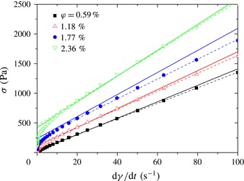
. The experimental and theoretical flow curves (shear stress versus shear rate dependences) are shown in figure 2 for four different CNT volume fractions
 $\unicode[STIX]{x1D719}$
ranging from 0.59 % to 2.36 %. First, we remark that the experimental flow curves (symbols in figure 2) have a rounded shape corresponding to a power-law behaviour at low shear rates
 $\dot{\unicode[STIX]{x1D6FE}}<10~\text{s}^{-1}$
followed by a linear segment at higher shear rates
 $\dot{\unicode[STIX]{x1D6FE}}>10~\text{s}^{-1}$
. Thus, the shear stress of CNT suspensions can be described by the Binhgam law,
 $\unicode[STIX]{x1D70E}_{12}=\unicode[STIX]{x1D70E}_{Y}+\unicode[STIX]{x1D702}_{s}\dot{\unicode[STIX]{x1D6FE}}$
, at
 $\dot{\unicode[STIX]{x1D6FE}}>10~\text{s}^{-1}$
, with the apparent shear yield stress
 $\unicode[STIX]{x1D70E}_{Y}$
obtained by a linear extrapolation of the flow curves to zero shear rate. This yield stress should not be confounded with the real yield stress which appears in some structured fluids and is considered to be the threshold stress required for the onset of flow when the structure breaks or starts to slip on the rheometer walls (Barnes Reference Barnes1999). Qualitatively, our model (solid lines in figure 2) reproduces the linear segments of the flow curves but fails to capture the initial rounded segment. This is probably because we ignore particle aggregation. This phenomenon should seriously impact the suspension rheology at low shear rates. The aggregate size is expected to decrease with increasing shear rate, resulting in a shear thinning manifested by the rounded shape of the flow curves. All of the aggregates are expected to be broken at high shear rates. Individual particles continue to interact with each other at high shear rates and result in linear segments of the flow curves. Thus, our model can be applied safely only for high enough shear rates corresponding to the non-aggregated state.
Experimental and theoretical flow curves of CNT suspensions at different particle volume fractions
 $\unicode[STIX]{x1D719}$
. The symbols correspond to experimental data of Natale et al. (Reference Natale, Heuzey, Carreau, Ausias and Férec2014), the dashed lines to the linear fit of the experimental data in the shear rate range
 $10~\text{s}^{-1}\leqslant \dot{\unicode[STIX]{x1D6FE}}\leqslant 100~\text{s}^{-1}$
and the solid lines to the theory ((2.26) with
 $k=25$
and
 $\unicode[STIX]{x1D707}F=7.5\times 10^{-13}~\text{N}$
). The values of the suspension volume fraction
 $\unicode[STIX]{x1D719}$
are given in the legend.

Quantitatively, the model fits reasonably well the experimental data of Natale et al. (Reference Natale, Heuzey, Carreau, Ausias and Férec2014) at
 $\dot{\unicode[STIX]{x1D6FE}}>10~\text{s}^{\text{-1}}$
. According to (2.26), the two free parameters used for the fit of the flow curves are the product
 $\unicode[STIX]{x1D707}F$
of the friction coefficient and the colloidal force, and the dimensionless constant
 $k$
intervening in (2.2) for the lubrication force. The best fit is obtained for
 $k=25$
and
 $\unicode[STIX]{x1D707}F=7.5\times 10^{-13}~\text{N}$
.
3.2 First normal stress difference
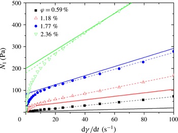
Experimental and theoretical (data of Natale et al. (Reference Natale, Heuzey, Carreau, Ausias and Férec2014)) shear rate dependences of the first normal stress difference for four different CNT volume fractions are plotted in figure 3. The experimental dependences (symbols in figure 3) show a similar trend to the flow curves plotted in figure 2. The normal stress difference seems to be insignificant at zero shear rate; a smooth power-law increase of the normal stress at low shear rates
 $\dot{\unicode[STIX]{x1D6FE}}<30~\text{s}^{-1}$
is followed by a linear segment at higher shear rates
 $\dot{\unicode[STIX]{x1D6FE}}>30~\text{s}^{-1}$
. Thus, at
 $\dot{\unicode[STIX]{x1D6FE}}>30~\text{s}^{-1}$
the experimental dependences can be fitted by a linear trend
 $N_{1}=N_{Y}+\unicode[STIX]{x1D702}_{n}\dot{\unicode[STIX]{x1D6FE}}$
similar to the Bingham law for the shear stress. The apparent normal yield stress
 $N_{Y}$
is found by a linear extrapolation of the experimental
 $N_{1}$
versus
 $\dot{\unicode[STIX]{x1D6FE}}$
dependences to zero shear rate. The relative yield contribution
 $N_{Y}/N_{1}$
to the normal stress appears to be more important than that
 $\unicode[STIX]{x1D70E}_{Y}/\unicode[STIX]{x1D70E}_{12}$
to the shear stress. This means that colloidal forces have a greater effect on the normal stress than on the shear stress. This could explain the difference between the shear rates
 $\dot{\unicode[STIX]{x1D6FE}}\approx 30~\text{s}^{-1}$
and
 $\dot{\unicode[STIX]{x1D6FE}}\approx 10~\text{s}^{-1}$
corresponding to the onset of the linear rheological behaviour of the normal and shear stresses respectively.
Experimental and theoretical shear rate dependences of the first normal stress difference for CNT suspensions at different particle volume fractions
 $\unicode[STIX]{x1D719}$
. The symbols correspond to experimental data of Natale et al. (Reference Natale, Heuzey, Carreau, Ausias and Férec2014), the dashed lines to the linear fit of the experimental data in the shear rate range
 $30~\text{s}^{-1}\leqslant \dot{\unicode[STIX]{x1D6FE}}\leqslant 100~\text{s}^{-1}$
and the solid lines to the theory (2.27). The suspension volume fraction
 $\unicode[STIX]{x1D719}$
is given in the legend.

The experimental curves were fitted by (2.27) of our model with the free parameters
 $k$
,
 $\unicode[STIX]{x1D707}F$
and
 $C$
. The fit was performed over the linear segment of the
 $N_{1}$
versus
 $\dot{\unicode[STIX]{x1D6FE}}$
dependence since our model ignores particle aggregation which, as explained before, is probably responsible for the rounded shape of the experimental curves at low shear rate. The values of the first two parameters were taken to be the same as for the fitting of the flow curves:
 $k=25$
and
 $\unicode[STIX]{x1D707}F=7.5\times 10^{-13}~\text{N}$
. Thus, the fit was performed using the remaining free parameter – the dimensionless constant
 $C$
appearing in (2.16) for the rotary diffusivity. The best fit corresponds to the value
 $C=3.7\times 10^{-5}$
. Strictly speaking, the weak-diffusion limit is hardly satisfied: at the highest volume fraction, we get
 $C\unicode[STIX]{x1D719}r_{e}^{3}\approx 0.6$
instead of
 $C\unicode[STIX]{x1D719}r_{e}^{3}\ll 1$
assumed in the model. However, numerical resolution of the Fokker–Planck equation shows that the approximation
 $C\unicode[STIX]{x1D719}r_{e}^{3}\ll 1$
still gives reasonable estimates of the moments
 $\langle \boldsymbol{p}\boldsymbol{p}\boldsymbol{p}\boldsymbol{p}\rangle$
up to
 $C\unicode[STIX]{x1D719}r_{e}^{3}\sim 1$
. For more quantitative comparison with experiments, we performed a linear fit of the experimental data in the shear rate range
 $30~\text{s}^{-1}\leqslant \dot{\unicode[STIX]{x1D6FE}}\leqslant 100~\text{s}^{-1}$
, individually for each particle concentration (cf. the dashed lines in figure 3). As is seen from figure 3, the model seems to correctly predict the apparent normal yield stress
 $N_{Y}$
(ordinate at the origin) but gives poorer predictions for the slopes of the
 $N_{1}$
versus
 $\dot{\unicode[STIX]{x1D6FE}}$
dependences.
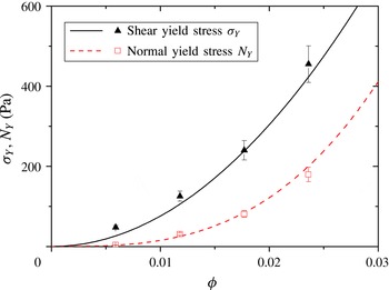
Experimental and theoretical dependences of the shear and normal apparent yield stresses on particle volume fraction. Symbols correspond to the experiments of Natale et al. (Reference Natale, Heuzey, Carreau, Ausias and Férec2014) and solid lines to the theory.

3.3 Apparent yield stress
In order to better analyse the apparent yield stress predicted by our model, the concentration dependences of both the shear and normal yield stresses are plotted in figure 4. The experimental points are obtained as the ordinates at the origins of the lines corresponding to individual linear fits of each experimental curve
 $\unicode[STIX]{x1D70E}(\dot{\unicode[STIX]{x1D6FE}})$
or
 $N_{1}(\dot{\unicode[STIX]{x1D6FE}})$
(dashed lines in figures 2 and 3). The theoretical concentration dependences
 $\unicode[STIX]{x1D70E}_{Y}(\unicode[STIX]{x1D719})$
and
 $N_{1}(\unicode[STIX]{x1D719})$
are calculated using (2.29) and (2.30). Figure 4 shows a relatively good correspondence between the experiments of Natale et al. (Reference Natale, Heuzey, Carreau, Ausias and Férec2014) and our model. Therefore, we may conclude that our model is able to capture the concentration effect on the apparent yield stress of the CNT suspension: according to (2.29) and (2.30), the shear yield stress is proportional to the concentration squared,
 $\unicode[STIX]{x1D70E}_{Y}\propto \unicode[STIX]{x1D719}^{2}$
, while the normal yield stress is proportional to the third power of the concentration,
 $N_{Y}\propto \unicode[STIX]{x1D719}^{3}$
. From the theoretical point of view, the
 $\unicode[STIX]{x1D70E}_{Y}\propto \unicode[STIX]{x1D719}^{2}$
behaviour comes from the pairwise interactions between fibres, and the
 $N_{Y}\propto \unicode[STIX]{x1D719}^{3}$
behaviour is the result of the combination of pair interactions (giving a
 $\unicode[STIX]{x1D719}^{2}$
contribution to the stress) and rotational diffusivity linear in
 $\unicode[STIX]{x1D719}$
(cf. (2.16)).
In the experiments of Natale et al. (Reference Natale, Heuzey, Carreau, Ausias and Férec2014), the shear stress seems to be insignificant at zero shear rate (cf. figure 2), so the suspension does not exhibit any real shear yield stress. Thus, until now we have analysed the apparent yield stress obtained as an intercept of the linear extrapolation of the experimental flow curves onto zero shear rate. However, some other authors report the real yield behaviour of CNT/epoxy suspensions, corresponding to the onset of flow (Rahatekar et al.
Reference Rahatekar, Koziol, Kline, Hobbie, Gilman and Windle2009; Hobbie Reference Hobbie2010). This real yield stress probably appears as a result of stronger colloidal interactions than those between the CNTs used in Natale’s experiments. Two considered types of CNTs have quite different diameters and aspect ratios (
 $D=16~\text{nm}$
and
 $r=160$
in Natale’s experiments, and
 $D=50~\text{nm}$
and
 $r=1200$
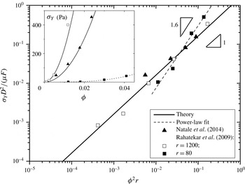
and 80 in Rahatekar’s experiments), and, as a consequence, quite different stress levels. Therefore, to compare the three sets of experimental data with our theory, it is convenient to introduce a dimensionless shear yield stress,
 $\unicode[STIX]{x1D70E}_{Y}D^{2}/(\unicode[STIX]{x1D707}F)$
, normalized by a characteristic ‘interaction’ stress
 $\unicode[STIX]{x1D707}F/D^{2}$
. Our model (2.29) predicts that the dimensionless yields stress scales as
 $\unicode[STIX]{x1D70E}_{Y}D^{2}/(\unicode[STIX]{x1D707}F)=16\unicode[STIX]{x1D719}^{2}r/\unicode[STIX]{x03C0}^{2}\propto \unicode[STIX]{x1D719}^{2}r$
. To check whether this tendency holds for the three sets of experimental data, we plot in figure 5 the experimental and theoretical dependences of the dimensionless yield stress on the factor
 $\unicode[STIX]{x1D719}^{2}r$
.
Dimensionless apparent yield stress as a function of
 $\unicode[STIX]{x1D719}^{2}r$
. The inset shows the dependence of the dimensional yield stress on particle concentration for the three sets of experimental data (symbols). The solid lines represent theoretical fits to the experimental data of Rahatekar et al. (Reference Rahatekar, Koziol, Kline, Hobbie, Gilman and Windle2009) and Natale et al. (Reference Natale, Heuzey, Carreau, Ausias and Férec2014), while the dashed line is a power-law fit to the data of Rahatekar et al. (Reference Rahatekar, Koziol, Kline, Hobbie, Gilman and Windle2009) for a CNT aspect ratio of
 $r=80$
.

The experimental values of the dimensionless yield stress have been obtained by fitting the experimental curves to the theoretical ones using the product
 $\unicode[STIX]{x1D707}F$
as a single adjustable parameter. The best fit corresponds to the values
 $\unicode[STIX]{x1D707}F=3\times 10^{-12}~\text{N}$
and
 $2.1\times 10^{-13}~\text{N}$
for
 $r=1200$
and 80 in Rahatekar’s experiments, while
 $\unicode[STIX]{x1D707}F=7.5\times 10^{-13}~\text{N}$
for Natale’s data with
 $r=160$
(the same value has been used above for the fit of Natale’s data shown in figures 2–4), The inset of figure 5 shows a concentration dependence of the dimensional yield stress. As inferred from this figure, the experimental data for the highest aspect ratios
 $r=160$
and 1200 respect the
 $\unicode[STIX]{x1D719}^{2}r$
behaviour predicted by our model for the dimensionless yield stress. The concentration dependence of the dimensional yield stress is also correctly predicted for these two sets of data. For the shorter particles,
 $r=80$
, used in Rahatekar’s experiments, a stronger concentration behaviour is observed. More precisely, the dimensional yield stress is best fitted by a power-law trend with an exponent 3.2 (
 $\unicode[STIX]{x1D70E}_{Y}\propto \unicode[STIX]{x1D719}^{3.2}$
, dashed line in the inset of figure 5). This gives the exponent 1.6 of the dimensionless yield stress versus
 $\unicode[STIX]{x1D719}^{2}r$
(i.e.
 $\unicode[STIX]{x1D70E}_{Y}D^{2}/(\unicode[STIX]{x1D707}F)\propto (\unicode[STIX]{x1D719}^{2}r)^{1.6}$
, dashed line in figure 5). This discrepancy with our theory is probably connected to strong aggregation (ignored in the model) of the CNTs with
 $r=80$
, while, at
 $r=1200$
, the suspension is much less aggregated, as revealed by optical microscopy imaging reported by Rahatekar et al. (Reference Rahatekar, Koziol, Kline, Hobbie, Gilman and Windle2009).
The value of the product
 $\unicode[STIX]{x1D707}F$
found by the fit of the theoretical model to experimental results allows estimation of the average separation
 $h$
between particle surfaces at the contact points. The electrostatic repulsion between untreated CNTs, used in Natale and Rahatekar’s experiments, is expected to be negligible, and the value of
 $h$
is retrieved from (2.6) with a zero second term on the right-hand side, namely
 $h=(AD/12F)^{1/2}$
. Thus, using a value of
 $\unicode[STIX]{x1D707}=0.3$
for the friction coefficient (Petrich & Koch Reference Petrich and Koch1998) and
 $A\sim 10^{-20}~\text{J}$
for the Hamaker constant (see appendix B), we obtain the value
 $h\approx 2.3~\text{nm}$
for
 $r=160$
and
 $D=16~\text{nm}$
(Natale’s data) and
 $h\approx 2.0~\text{nm}$
for
 $r=1200$
and
 $D=50~\text{nm}$
(Rahatekar’s data). These values seem to be realistic and satisfy the limit of validity
 $h\ll D$
of assumptions (4) and (5) of § 2.1.
It is also worth noticing that in the general case of 3D shear or extensional flows, our model predicts an anisotropic yield stress, as follows (see the last term of (2.25)):
 $$\begin{eqnarray}\displaystyle & \displaystyle \unicode[STIX]{x1D70E}_{ik}^{Y}=\frac{8}{3\unicode[STIX]{x03C0}^{2}}\unicode[STIX]{x1D719}^{2}\frac{\unicode[STIX]{x1D707}F}{D^{2}}r\frac{\langle p_{i}p_{k}p_{l}p_{m}\rangle }{\langle \hat{u} \rangle }\hat{\unicode[STIX]{x1D6FE}}_{lm}, & \displaystyle\end{eqnarray}$$
 $$\begin{eqnarray}\displaystyle & \displaystyle \langle \hat{u} \rangle =\frac{\langle |\boldsymbol{u}|\rangle }{L\dot{\unicode[STIX]{x1D6FE}}}=\frac{1}{L^{3}\dot{\unicode[STIX]{x1D6FE}}}\int _{\boldsymbol{p}^{\unicode[STIX]{x1D6FC}}}\unicode[STIX]{x1D713}_{\unicode[STIX]{x1D6FC}}\,\text{d}\boldsymbol{p}^{\unicode[STIX]{x1D6FC}}\int _{\boldsymbol{p}^{\unicode[STIX]{x1D6FD}}}\unicode[STIX]{x1D713}_{\unicode[STIX]{x1D6FD}}\,\text{d}\boldsymbol{p}^{\unicode[STIX]{x1D6FD}}\int _{-L/2}^{L/2}\int _{-L/2}^{L/2}|\boldsymbol{u}|\,\text{d}s_{\unicode[STIX]{x1D6FC}}\,\text{d}s_{\unicode[STIX]{x1D6FD}}, & \displaystyle\end{eqnarray}$$
where
 $\hat{\unicode[STIX]{x1D6FE}}_{lm}=\unicode[STIX]{x1D6FE}_{lm}/\dot{\unicode[STIX]{x1D6FE}}$
. In the particular case of simple shear flow in the low-diffusion limit, considered in the present paper, equation (3.2) for
 $\langle \hat{u} \rangle$
reduces to (2.24). Our expression (3.1) for the yield stress tensor differs from the one derived recently by Férec et al. (Reference Férec, Perrot and Ausias2015),
 $$\begin{eqnarray}\displaystyle & \displaystyle \unicode[STIX]{x1D70E}_{ik}^{Y}=\frac{8}{\unicode[STIX]{x03C0}^{2}}\unicode[STIX]{x1D719}^{2}k\frac{K}{D}r\left\langle \frac{p_{i}p_{k}p_{l}p_{m}\sin \unicode[STIX]{x1D6FF}}{\hat{u} }\right\rangle \hat{\unicode[STIX]{x1D6FE}}_{lm}, & \displaystyle\end{eqnarray}$$
 $$\begin{eqnarray}\displaystyle & \displaystyle \hat{u} =|p_{n}p_{s}\hat{\unicode[STIX]{x1D6FE}}_{ns}|, & \displaystyle\end{eqnarray}$$
where
 $K$
is the consistency measured in
 $\text{N}~\text{m}^{-1}$
,
 $k$
is the dimensionless interaction parameter describing the intensity of inter-fibre forces and
 $\sin \unicode[STIX]{x1D6FF}=|\boldsymbol{p}^{\unicode[STIX]{x1D6FC}}\times \boldsymbol{p}^{\unicode[STIX]{x1D6FD}}|$
(cf. figure 1). The last expression was derived by setting to zero the value of the power-law index
 $\unicode[STIX]{x1D705}$
in the phenomenological expression
 $\boldsymbol{F}\propto |\boldsymbol{u}|^{\unicode[STIX]{x1D705}-1}\boldsymbol{u}$
for the interaction force between fibres. The physical meaning of the consistency
 $K$
was not clarified. In contrast to the phenomenological approach adopted in this previous model, the present model introduces realistic physical interactions between fibres (colloidal, solid friction and lubrication forces), and predicts the yield stress tensor in terms of the friction force. Comparing (3.1) and (3.3), we are able to identify the scaling of the consistency in the model of Férec et al. (Reference Férec, Perrot and Ausias2015) in terms of measurable physical quantities:
 $K=O(\unicode[STIX]{x1D707}F/D)$
. Another difference consists of the fact that the orientation tensor in (3.3) contains the Onsager potential
 $\sin \unicode[STIX]{x1D6FF}=|\boldsymbol{p}^{\unicode[STIX]{x1D6FC}}\times \boldsymbol{p}^{\unicode[STIX]{x1D6FD}}|$
since, in the model of Férec et al. (Reference Férec, Perrot and Ausias2015), the interaction force is not supposed to be inversely proportional to
 $|\boldsymbol{p}^{\unicode[STIX]{x1D6FC}}\times \boldsymbol{p}^{\unicode[STIX]{x1D6FD}}|$
, like in the present theory (cf. the discussion below (2.25)). Finally, the two models use different assumptions for the estimation of the absolute value
 $|\boldsymbol{u}|$
of the relative velocity of the fibres (cf. (2.23), (2.24) and (3.2) for the present model and (3.4) for the model of Férec et al. (Reference Férec, Perrot and Ausias2015)). It should be noticed that both models produce the same concentration behaviour of the yield stress,
 $\unicode[STIX]{x1D70E}_{Y}\propto \unicode[STIX]{x1D719}^{2}$
, for pair-wise interactions.
Regarding the aspect-ratio effect, it should be recalled that the current model is developed for the high-aspect-ratio limit
 $r\gg 1$
, predicting the shear yield stress proportional to
 $r$
. The model is unable to provide quantitative predictions for lower aspect ratios, say
 $r<10$
. However, qualitatively, the mean number of contact points per particle (coordination number) is much higher for long fibres than for spheres, at the same particle volume fraction. Therefore, at particle concentrations as low as
 $\unicode[STIX]{x1D719}=0.02$
, the effect of van der Waals forces is expected to be much lower for spherical-particle suspensions than for long-fibre suspensions.
4 Concluding remarks
This work is focused on the modelling of the shear and normal stresses in fibre suspensions that are subjected to a simple shear flow in the presence of short-range lubrication and overall attractive colloidal forces between fibres. The static friction force between fibres is also taken into account and supposed to be proportional to the attractive resultant colloidal force. The model is applied to the experimental data of Rahatekar et al. (Reference Rahatekar, Koziol, Kline, Hobbie, Gilman and Windle2009) and Natale et al. (Reference Natale, Heuzey, Carreau, Ausias and Férec2014) on suspensions of CNT dispersed in a Newtonian epoxy resin; however, it can also be used for other rod-like particle suspensions with attractive interactions.
The contact lubrication and solid friction forces are estimated in a simple Cartesian reference frame and result in objective orientation and stress tensors. Following the approach of Djalili-Moghaddam & Toll (Reference Djalili-Moghaddam and Toll2005) and Férec et al. (Reference Férec, Ausias, Heuzey and Carreau2009), these forces are averaged over the contact probability. The mean force exerted by neighbouring fibres on a test fibre appears to be zero and results in an affine translational motion. Furthermore, the deterministic angular motion of fibres is also unaffected by the short-range forces, in agreement with Djalili-Moghaddam & Toll (Reference Djalili-Moghaddam and Toll2005), as opposed to the work of Férec et al. (Reference Férec, Ausias, Heuzey and Carreau2009) who have used the co-rotational frame. These conclusions apply only under the assumption of perfect sliding contacts at all contact points. The presence of sticky contacts should promote the formation of a fibre network (Switzer & Klingenberg Reference Switzer and Klingenberg2004). As a consequence, this could break the affinity of the translational motion and affect the rotational motion. Such an aggregation scenario is ignored in the present model.
The short-ranged interactions could, in principle, influence the rotary diffusivity of fibres and affect their stochastic rotational motion. However, in the weak-diffusion
 $D_{r}r_{e}^{3}/\dot{\unicode[STIX]{x1D6FE}}\ll 1$
and high-aspect-ratio
 $r\gg 1$
limits employed in the present work, the rotary diffusivity does not intervene in the component
 $\langle p_{1}^{2}p_{2}^{2}\rangle$
of the orientation tensor appearing in the shear stress but does in the goniometric factor
 $\langle p_{1}^{3}p_{2}\rangle -\langle p_{1}p_{2}^{3}\rangle$
appearing in the first normal stress difference. The effect of the colloidal interactions on the rotary diffusivity was neglected. The combined effect of the long- and short-ranged hydrodynamic interactions was taken into account in a phenomenological way, assuming
 $D_{r}\propto \unicode[STIX]{x1D719}\dot{\unicode[STIX]{x1D6FE}}$
. In this way, the factor
 $\langle p_{1}^{3}p_{2}\rangle -\langle p_{1}p_{2}^{3}\rangle$
appeared to be independent of the shear rate and proportional to the particle concentration.
The particle stress was shown to be the sum of two contributions as follows: (1) the stress coming from hydrodynamic interaction between the fibres and the suspending liquid (with the rheological coefficients borrowed from the slender-body theory in the dilute limit); (2) the stress coming from solid friction between fibres and proportional to the resultant attractive colloidal force. In the considered experimental conditions (Natale et al.
Reference Natale, Heuzey, Carreau, Ausias and Férec2014), the lubrication force does not seem to provide any direct contribution to the particle stress but may influence the rotary diffusivity of the fibres. Our model predicts a simple Bingham law for both the shear stress and the first normal stress difference, with the apparent shear and normal yield stresses proportional to
 $\unicode[STIX]{x1D719}^{2}$
and
 $\unicode[STIX]{x1D719}^{3}$
respectively. The
 $\unicode[STIX]{x1D70E}_{Y}\propto \unicode[STIX]{x1D719}^{2}$
trend is explained by pair colloidal interactions between fibres. The behaviour
 $N_{1}\propto \unicode[STIX]{x1D719}^{2}(\langle p_{1}^{3}p_{2}\rangle -\langle p_{1}p_{2}^{3}\rangle )\propto \unicode[STIX]{x1D719}^{3}$
stands for the synergy between the attractive colloidal forces (responsible for the
 $\unicode[STIX]{x1D719}^{2}$
contribution) and hydrodynamic interactions, implicitly included in the rotary diffusivity and giving
 $\langle p_{1}^{3}p_{2}\rangle -\langle p_{1}p_{2}^{3}\rangle \propto \unicode[STIX]{x1D719}$
. The second normal stress difference is negligible with respect to the first normal stress difference in the same way as in non-Brownian suspensions where fibres interact only through hydrodynamic forces (Larson Reference Larson1999).
The experiments on CNT suspensions also reveal apparent Bingham behaviour. The model captures well the quadratic concentration behaviour of the yield stress for the long CNT particles used in the Rahatekar et al. (Reference Rahatekar, Koziol, Kline, Hobbie, Gilman and Windle2009) experiments (
 $r=1200$
) and the Natale et al. (Reference Natale, Heuzey, Carreau, Ausias and Férec2014) experiments (
 $r=160$
), but fails to predict the
 $\unicode[STIX]{x1D719}^{3.2}$
trend for the shorter CNTs,
 $r=80$
, used by Rahatekar, probably because of the strong aggregation observed for those particles. The flow curves in Natale’s experiments have a rounded shape at low shear rates, while our model predicts a linear shape with a pronounced yield stress. This discrepancy is tentatively explained by aggregation at low shear rates ignored by the present model. Besides all the simplifications, the model fits reasonably well to experimental
 $\unicode[STIX]{x1D70E}_{12}$
versus
 $\dot{\unicode[STIX]{x1D6FE}}$
and
 $N_{1}$
versus
 $\dot{\unicode[STIX]{x1D6FE}}$
dependences at high shear rates (
 $\dot{\unicode[STIX]{x1D6FE}}>10~\text{s}^{-1}$
for
 $\unicode[STIX]{x1D70E}_{12}$
and
 $\dot{\unicode[STIX]{x1D6FE}}>30~\text{s}^{-1}$
for
 $N_{1}$
). This is a positive argument for the validity of our non-aggregation approach. In the future, we plan to construct a more realistic model taking into account both imperfect sliding and particle aggregation. This future model should allow us to capture the rounded shape of the flow curves at low shear rates. It would combine the features of the present microscopic approach (allowing a rather rigorous determination of the contact forces) with macroscopic aggregation–orientation models proposed by Ma et al. (Reference Ma, Chinesta, Ammar and Mackley2008) and Abisset-Chavanne et al. (Reference Abisset-Chavanne, Chinesta, Ferec, Ausias and Keunings2015).
Acknowledgements
The authors are grateful to Professors P. J. Carreau and M. C. Heuzey of Polytechnique Montréal and Dr G. Natale from the University of Calgary for providing the experimental data. They would also like to acknowledge Région Provence – Alpes Côte d’Azur which funded one of them. This work was also supported by the Program of the Ministry of Education of the Russian Federation (project no. 3.12.2014/K).
Appendix A. Demonstration of (2.20)–(2.21) for the stress tensor
The particle stress averaged over the contact probability but not yet averaged over the fibre orientation reads (Pokrovskiy Reference Pokrovskiy1978; Landau & Lifshitz Reference Landau and Lifshitz1987)
 $$\begin{eqnarray}\displaystyle \langle \unicode[STIX]{x1D70E}_{ik}^{p}\rangle _{P} & = & \displaystyle n\oint _{S_{\mathit{particle}}}\unicode[STIX]{x1D70E}_{il}n_{l}x_{k}\,\text{d}S=\underbrace{n\oint _{S_{\mathit{particle}}}\unicode[STIX]{x1D70E}_{il}^{long}n_{l}x_{k}\,\text{d}S}_{\substack{ \text{contribution from long-ranged} \\ \text{hydrodynamic forces}}}+\underbrace{n\oint _{S_{\mathit{particle}}}\unicode[STIX]{x1D70E}_{il}^{stoch}n_{l}x_{k}\,\text{d}S}_{\substack{ \text{contribution from} \\ \text{stochastic torque} \\ \text{(rotary diffusion)}}}\nonumber\\ \displaystyle & & \displaystyle +\,\underbrace{n\oint _{S_{\mathit{particle}}}\unicode[STIX]{x1D70E}_{il}^{short}n_{l}x_{k}\,\text{d}S}_{\substack{ \text{contribution from} \\ \text{short-ranged forces}}}\nonumber\\ \displaystyle & = & \displaystyle \underbrace{nV_{f}\unicode[STIX]{x1D702}_{0}\left\{4\unicode[STIX]{x1D6FE}_{ik}+\frac{\unicode[STIX]{x1D6FD}f^{\Vert }}{2}\left[p_{i}p_{k}p_{l}p_{m}-\frac{1}{3}\unicode[STIX]{x1D6FF}_{ik}p_{l}p_{m}\right]\unicode[STIX]{x1D6FE}_{lm}\right\}-\frac{1}{2}n\{p_{i}p_{l}\unicode[STIX]{x1D61B}_{lk}^{hydro}+p_{k}p_{l}\unicode[STIX]{x1D61B}_{li}^{hydro}\}+\frac{1}{2}n\unicode[STIX]{x1D61B}_{ik}^{hydro}}_{\text{contribution from long-ranged hydrodynamic forces}}\nonumber\\ \displaystyle & & \displaystyle +\,\underbrace{nV_{f}\unicode[STIX]{x1D6FD}f^{\bot }\unicode[STIX]{x1D702}_{0}D_{r}p_{k}\frac{\unicode[STIX]{x2202}\ln \unicode[STIX]{x1D713}}{\unicode[STIX]{x2202}p_{i}}}_{\text{contribution from rotary diffusion}}+\underbrace{np_{k}\underbrace{\int s_{\unicode[STIX]{x1D6FC}}F_{i}\,\text{d}P}_{\unicode[STIX]{x1D711}_{i}}}_{\substack{ \text{contribution from} \\ \text{short-ranged forces}}}\nonumber\\ \displaystyle & = & \displaystyle {\unicode[STIX]{x1D70E}_{ik}}_{0}^{p}-\frac{1}{2}n\{p_{i}p_{l}\unicode[STIX]{x1D61B}_{lk}^{hydro}+p_{k}p_{l}\unicode[STIX]{x1D61B}_{li}^{hydro}\}+\frac{1}{2}n\unicode[STIX]{x1D61B}_{ik}^{hydro}+\frac{1}{2}n(\unicode[STIX]{x1D711}_{i}p_{k}+\unicode[STIX]{x1D711}_{k}p_{i})+\frac{1}{2}n(\unicode[STIX]{x1D711}_{i}p_{k}-\unicode[STIX]{x1D711}_{k}p_{i}),\end{eqnarray}$$
 $$\begin{eqnarray}{\unicode[STIX]{x1D70E}_{ik}}_{0}^{p}=nV_{f}\unicode[STIX]{x1D702}_{0}\left\{4\unicode[STIX]{x1D6FE}_{ik}+\frac{\unicode[STIX]{x1D6FD}f^{\Vert }}{2}\left[p_{i}p_{k}p_{l}p_{m}-\frac{1}{3}\unicode[STIX]{x1D6FF}_{ik}p_{l}p_{m}\right]\unicode[STIX]{x1D6FE}_{lm}\right\}+nV_{f}\unicode[STIX]{x1D6FD}f^{\bot }\unicode[STIX]{x1D702}_{0}D_{r}p_{k}\frac{\unicode[STIX]{x2202}\ln \unicode[STIX]{x1D713}}{\unicode[STIX]{x2202}p_{i}},\end{eqnarray}$$
where
 $\unicode[STIX]{x1D61B}_{ik}^{hydro}$
is the ‘
 $ik$
’ component of the tensor of the hydrodynamic torque acting on the fibres,
 $\unicode[STIX]{x1D713}$
is the orientation distribution function,
 ${\unicode[STIX]{x1D70E}_{ik}}_{0}^{p}$
is the stress generated by a test fibre at zero hydrodynamic torque in the absence of the short-ranged forces,
 $\unicode[STIX]{x1D711}_{i}=\int s_{\unicode[STIX]{x1D6FC}}F_{i}\,\text{d}P$
and other terms are explained below (2.20)–(2.21). The torque balance on a given fibre reads
 $$\begin{eqnarray}\unicode[STIX]{x1D61B}_{ik}^{hydro}+(\unicode[STIX]{x1D711}_{i}p_{k}-\unicode[STIX]{x1D711}_{k}p_{i})=0.\end{eqnarray}$$
Using this expression, we can show that
 $$\begin{eqnarray}{\textstyle \frac{1}{2}}n\{p_{i}p_{l}\unicode[STIX]{x1D61B}_{lk}^{hydro}+p_{k}p_{l}\unicode[STIX]{x1D61B}_{li}^{hydro}\}={\textstyle \frac{1}{2}}n(\unicode[STIX]{x1D711}_{i}p_{k}+\unicode[STIX]{x1D711}_{k}p_{i})-np_{i}p_{k}p_{l}\unicode[STIX]{x1D711}_{l}.\end{eqnarray}$$
Substituting (A 3), (A 4) into (A 1) gives
 $$\begin{eqnarray}\langle \unicode[STIX]{x1D70E}_{ik}^{p}\rangle _{P}={\unicode[STIX]{x1D70E}_{ik}}_{0}^{p}+np_{i}p_{k}p_{l}\unicode[STIX]{x1D711}_{l}.\end{eqnarray}$$
The second term here stands for the longitudinal stress generated by short-ranged forces on the fibres and is given by (A 2). Substituting (A 2) into (A 5), averaging over all possible fibre orientations and adding the solvent contribution we arrive at the final expression (2.20)–(2.21) for the stress tensor in the suspension.
Appendix B. Estimation of the Hamaker constant
The Hamaker constant for CNT/epoxy composites can be estimated using simplified Lifshitz theory applied to the case of non-retarded van der Waals interaction and completely screened electrostatic interaction (Russell, Saville & Schowalter Reference Russell, Saville and Schowalter1989):
 $$\begin{eqnarray}A\approx \frac{3\hslash \unicode[STIX]{x1D714}_{UV}}{16\sqrt{2}}\frac{(n_{f}^{2}-n_{s}^{2})^{2}}{(n_{f}^{2}+n_{s}^{2})^{3/2}},\end{eqnarray}$$
where
 $\hslash =1.055\times 10^{-34}~\text{J}~\text{s}$
is the Planck constant,
 $\unicode[STIX]{x1D714}_{UV}\approx 7.2\times 10^{-15}~\text{rad}~\text{s}^{-1}$
is the frequency of dominant relaxation of CNTs in the ultraviolet region, and
 $n_{f}\approx 2.15$
and
 $n_{s}\approx 1.57$
are the refractive indices of CNT particles and epoxy matrix respectively (Khalkhal et al.
Reference Khalkhal, Carreau and Ausias2011). Estimations give a value of
 $A\sim 10^{-20}~\text{J}$
.