1 Introduction
Waves at the interface of two immiscible viscous fluids have been of interest to the fluid dynamics community for technological applications such as drug delivery (Tsai et al. Reference Tsai, Mao, Lin, Zhu and Tsai2014) as well as from a fundamental perspective in understanding nonlinear systems and phenomena such as atomisation (Puthenveettil & Hopfinger Reference Puthenveettil and Hopfinger2009; Li & Umemura Reference Li and Umemura2014). Dating from the seminal study by Michael Faraday (Faraday Reference Faraday1831), forced standing interfacial oscillations have received continued interest and attention in the fluid dynamics literature having become a canonical system for studying nonlinear physics and pattern formation in parametrically forced systems (Perinet, Juric & Tuckerman Reference Perinet, Juric and Tuckerman2009; Rajchenbach & Clamond Reference Rajchenbach and Clamond2015). A study of such oscillations, especially the ones occurring in cylindrical geometries, has significant practical utility. They appear during sloshing in partially liquid-filled cylindrical containers subject to vertical vibration (Henderson & Miles Reference Henderson and Miles1994). Atomisation as a result of instabilities of standing waves appearing on a vibrated sessile droplet have been proposed as a technique for spray cooling of microprocessors (James et al. Reference James, Vukasinovic, Smith and Glezer2003). Axisymmetric free interfacial oscillations similarly have many applications. At large scales, where surface tension and viscous effects are negligible, they are relevant for understanding seiches in harbours (Mack Reference Mack1962). The well-known Cauchy–Poisson problem in water waves (Debnath Reference Debnath1994) can be analysed as a linear superposition of axisymmetric standing modes excited by initial conditions (Miles Reference Miles1968). At smaller laboratory scales involving smaller wavelengths and highly viscous fluids, gravity, surface tension and viscosity can significantly influence the time evolution, deformation and subsequent break-up of these interfacial waves (Goodridge et al. Reference Goodridge, Shi, Hentschel and Lathrop1997). Early comparisons of experiments on standing waves with nonlinear, inviscid, irrotational theory were made by Taylor (Reference Taylor1953) and Thorpe (Reference Thorpe1968). A comparison of theoretical damping calculations of free oscillations with experiments was reported by Miles & Henderson (Reference Miles and Henderson1990) in a confined cylindrical geometry. For a highly viscous fluid viz. paraffin oil, Bechhoefer et al. (Reference Bechhoefer, Ego, Manneville and Johnson1995) conducted experiments on Faraday waves in cylinders finding that for sufficient size, oscillations behave as if they are occurring in radially unbounded geometry.
The dispersion relation for irrotational, small-amplitude interfacial waves on unbounded fluids in a planar geometry has been long known (Lamb Reference Lamb1932) and is readily obtainable from normal mode analysis. The addition of viscosity into the normal mode approximation was done by Harrison (Reference Harrison1908) (also see Lamb (Reference Lamb1932), Chandrasekhar (Reference Chandrasekhar1961)). The viscous normal mode eigenfunctions however do not form a complete set (Lamb Reference Lamb1932) and the spectrum has an additional continuous part, for which no dispersion relation exists (Lamb Reference Lamb1932; Balmforth & Morrison Reference Balmforth and Morrison1995). Thus one cannot solve the initial value problem (IVP) for general initial conditions by expanding these in the normal mode eigenfunctions alone. This lacuna was rectified in Prosperetti (Reference Prosperetti1976), Menikoff et al. (Reference Menikoff, Mjolsness, Sharp, Zemach and Doyle1978), Prosperetti (Reference Prosperetti1981) who solved the planar IVP for a single spatial Fourier mode using Laplace transform in time. It was demonstrated that in addition to normal mode terms arising from the discrete part of the spectrum, the viscous spectrum has a continuous part which leads to terms with non-exponential dependence on time. In a planar geometry and for capillary waves, a comparison of the IVP solution of Prosperetti (Reference Prosperetti1981) with direct numerical simulation (DNS) of the Navier–Stokes equation for small perturbation amplitude has been reported in Popinet (Reference Popinet2013), Denner (Reference Denner2016) and a good match has been observed. Using scaling arguments, Denner (Reference Denner2016) also showed that for small-amplitude under-damped capillary oscillations, independent of the viscosity and density ratio of the two fluids, a single non-dimensional frequency can be obtained for a given non-dimensional wavenumber. The critical wavenumber used for this collapse was obtained using a damped simple harmonic oscillator model for the interface. Further extension of this work to include finite-amplitude capillary waves has been recently reported in Denner, Paré & Zaleski (Reference Denner, Paré and Zaleski2017a ) where an empirical correlation is obtained for the effect of wave amplitude on viscous dissipation. Using this correlation to correct for finite-amplitude effects, it has been shown (Denner et al. Reference Denner, Paré and Zaleski2017a ) that the capillary wave dispersion relation is self-similar for finite-amplitude waves as well. In cylindrical axisymmetric radially bounded geometries, inviscid, irrotational interfacial oscillations have been analysed in Drazin & Reid (Reference Drazin and Reid2004) (see problem 1.12) using normal modes. In the presence of a confining cylindrical boundary, a viscous normal mode study has been reported in Sweeney, Kerswell & Mullin (Reference Sweeney, Kerswell and Mullin2013). The only study of the IVP for radially unbounded cylindrical geometry is by Miles (Reference Miles1968) who obtained analytical results for certain initial conditions. His solution however neglects the inertia and viscosity of the upper fluid, whose effect in certain parametric regimes can be large. The solution to the axisymmetric IVP involving inertia and viscosity of both fluids has not been reported in the literature before and is done here. It is shown that a small-amplitude axisymmetric Bessel mode temporally evolves in exactly the same way as a planar Fourier mode. Detailed comparisons of DNS results, the normal mode solution and the IVP for a range of non-dimensional parameters are reported here for the first time. The paper is organised as follows: In § 2 we solve the IVP. Results from the normal mode approximation are provided in § 3 followed by a description of simulations in § 4. Results, comparisons and analysis are presented in § 5. We conclude with a discussion and future scope of work.
2 Viscous initial value problem
In this section, we derive the equation governing the time evolution of the interface initiated as an axisymmetric zeroth-order Bessel’s function of the first kind. All fields (velocity, pressure etc.) are decomposed (Lamb Reference Lamb1932; Miles Reference Miles1968; Prosperetti Reference Prosperetti1976; Menikoff et al.
Reference Menikoff, Mjolsness, Sharp, Zemach and Doyle1978; Prosperetti Reference Prosperetti1981) into a potential part indicated with subscript
 $p$
and a viscous part (subscript
 $v$
). The sum of the two fields are constrained to satisfy appropriate continuity conditions at the interface (discussed later). Superscripts
 ${\mathcal{U}}$
and
 ${\mathcal{L}}$
are used to indicate upper and lower fluid respectively. Thus
 $\unicode[STIX]{x1D6EF}_{p}\text{}^{{\mathcal{U}}}$
represents the potential part of the field variable
 $\unicode[STIX]{x1D6EF}$
in the upper fluid and so on. The algebra is lengthy and hence only the outline is presented here along with the main results. A detailed step-by-step derivation is provided as see supplementary material available at https://doi.org/10.1017/jfm.2017.443 (Farsoiya, Mayya & Dasgupta Reference Farsoiya, Mayya and Dasgupta2017).
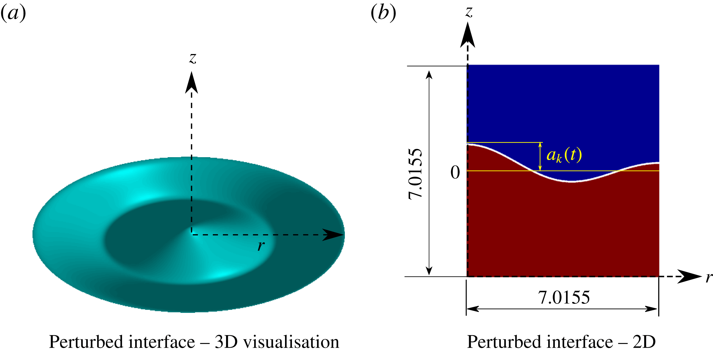
(a) The initial interface is
 $\unicode[STIX]{x1D702}(r,0)=a_{k}(0)\text{J}_{0}(kr)$
. The analytical study assumes unboundedness in the radial (
 $r$
) and axial (
 $z$
) directions. The three-dimensional image is for visualisation purposes only. (b) In DNS we use symmetry boundary conditions on all computational domain boundaries. Most of the simulations are done with a domain size
 $[0,7.01556]\times [0,7.01556]$
, see table 1. The left vertical boundary is the axis of symmetry.
 $a_{k}(t)$
is measured from the unperturbed interface represented by the horizontal line at level
 $0$
.

2.1 IVP – potential flow
Referring to figure 1(a), an axisymmetric interface between two immiscible fluids of density and viscosity
 $\unicode[STIX]{x1D70C}\text{}^{{\mathcal{L}}},\unicode[STIX]{x1D70C}\text{}^{{\mathcal{U}}}$
and
 $\unicode[STIX]{x1D707}\text{}^{{\mathcal{L}}},\unicode[STIX]{x1D707}\text{}^{{\mathcal{U}}}$
with surface tension coefficient
 $T$
is represented as a standing wave
 $$\begin{eqnarray}\unicode[STIX]{x1D702}(r,t)=a_{k}(t)\text{J}_{0}(kr),\end{eqnarray}$$
with
 $\unicode[STIX]{x1D702}(r,0)=a_{k}(0)\text{J}_{0}(kr)$
,
 $\text{J}_{0}(kr)$
being the zeroth-order Bessel function of the first kind. The radial dependence of all fields is chosen to be a Bessel function as these are eigenfunctions of the radial part of the Laplacian operator written in cylindrical coordinates. Our analysis is linear, retaining terms up to
 $O(a_{k}(0))$
as
 $a_{k}(0)\rightarrow 0$
. We consider a stable configuration with
 $\unicode[STIX]{x1D70C}\text{}^{{\mathcal{L}}}>\unicode[STIX]{x1D70C}\text{}^{{\mathcal{U}}}$
with both fluids being radially and vertically unbounded (
 $0\leqslant r\leqslant \infty$
and
 $-\infty \leqslant z\leqslant \infty$
) (in figure 1(b), the boundaries are for computational purposes only, as described later). Unlike normal mode analysis which assumes an exponential dependence on time (Lamb Reference Lamb1932), the temporal part of all quantities are taken to be unknown functions of time (Prosperetti Reference Prosperetti1976) in this analysis. For potential flow, we solve the axisymmetric Laplace equation in the velocity potential
 $\unicode[STIX]{x1D719}_{p}$
. Using variable separation in the Laplace equation, we find
 $$\begin{eqnarray}\unicode[STIX]{x1D719}_{p}\text{}^{{\mathcal{U}}}(r,z,t)=F(z)\text{J}_{0}(kr){\dot{a}}_{k}(t),\quad \unicode[STIX]{x1D719}_{p}\text{}^{{\mathcal{L}}}(r,z,t)=G(z)\text{J}_{0}(kr){\dot{a}}_{k}(t).\end{eqnarray}$$
where
 $F$
and
 $G$
are unknown functions of
 $z$
. A dot above
 $a_{k}$
indicates differentiation with respect time. We set the time dependence of
 $\unicode[STIX]{x1D719}_{p}$
equal to
 ${\dot{a}}_{k}(t)$
anticipating the linearised kinematic boundary condition at the interface (see Farsoiya et al.
Reference Farsoiya, Mayya and Dasgupta2017). Equations (2.2a,b
) when substituted into the axisymmetric Laplace equation (Kundu & Cohen Reference Kundu and Cohen2002), lead to equations for
 $F(z)$
and
 $G(z)$
. Using the boundedness condition on
 $F(z)$
and
 $G(z)$
and the linearised kinematic boundary condition, we obtain
 $$\begin{eqnarray}\unicode[STIX]{x1D719}_{p}\text{}^{{\mathcal{U}}}(r,z,t)=-k^{-1}\exp [-kz]\text{J}_{0}(kr){\dot{a}}_{k}(t),\quad \unicode[STIX]{x1D719}_{p}\text{}^{{\mathcal{L}}}(r,z,t)=k^{-1}\exp [kz]\text{J}_{0}(kr){\dot{a}}_{k}(t).\end{eqnarray}$$
The potential part of pressure in both the fluids is determined from the linearised Bernoulli equation.
 $$\begin{eqnarray}\left.\begin{array}{@{}c@{}}p\text{}_{p}^{{\mathcal{L}}}(r,0,t)=-\unicode[STIX]{x1D70C}\text{}^{{\mathcal{L}}}{\displaystyle \frac{\unicode[STIX]{x2202}\unicode[STIX]{x1D719}_{p}\text{}^{{\mathcal{L}}}}{\unicode[STIX]{x2202}t}}\bigg|_{z=0}-\unicode[STIX]{x1D70C}\text{}^{{\mathcal{L}}}ga_{k}(t)\text{J}_{0}(kr),\\ p\text{}_{p}^{{\mathcal{U}}}(r,0,t)=-\unicode[STIX]{x1D70C}\text{}^{{\mathcal{U}}}{\displaystyle \frac{\unicode[STIX]{x2202}\unicode[STIX]{x1D719}_{p}\text{}^{{\mathcal{U}}}}{\unicode[STIX]{x2202}t}}\bigg|_{z=0}-\unicode[STIX]{x1D70C}\text{}^{{\mathcal{U}}}ga_{k}(t)\text{J}_{0}(kr).\end{array}\right\}\end{eqnarray}$$
If we wish to consider potential flow only, then continuity of pressure at the interface (in the absence of surface tension) leads to a simple harmonic oscillator equation for
 $a_{k}(t)$
with frequency
 $\sqrt{(\unicode[STIX]{x1D70C}\text{}^{{\mathcal{L}}}-\unicode[STIX]{x1D70C}\text{}^{{\mathcal{U}}})gk/(\unicode[STIX]{x1D70C}\text{}^{{\mathcal{L}}}+\unicode[STIX]{x1D70C}\text{}^{{\mathcal{U}}})}$
.
2.2 IVP – viscous flow
Inclusion of viscous effects modifies the analysis considerably. It is known that viscous stresses are non-zero in a potential flow (Stokes Reference Stokes1851; Joseph Reference Joseph2003), and due to a jump in the viscosity across the interface, these stresses are discontinuous. In addition the tangential velocities are also discontinuous at the interface. Thus while potential flow satisfies the continuity and the Navier–Stokes equation (Joseph Reference Joseph2003) (also see Farsoiya et al.
Reference Farsoiya, Mayya and Dasgupta2017), it does not satisfy the boundary conditions. In order to satisfy these, an additional velocity and pressure field is necessary. The composite velocity and pressure fields
 $\boldsymbol{v}=\boldsymbol{v}_{p}+\boldsymbol{v}_{v}$
and
 $p=p_{p}+p_{v}$
satisfy both the governing equations as well as the boundary conditions. This composite velocity field
 $\boldsymbol{v}$
is rotational, with vorticity being generated at the interface. In a cylindrical axisymmetric coordinate system (see figure 1), (
 $\boldsymbol{v}\equiv (u,v)$
with
 $u$
the radial component and
 $v$
the axial component of velocity.) the composite velocity and pressure fields can be written as,
 $$\begin{eqnarray}\left.\begin{array}{@{}c@{}}u\text{}^{{\mathcal{U}}}=u_{p}\text{}^{{\mathcal{U}}}+u_{v}\text{}^{{\mathcal{U}}}={\displaystyle \frac{\unicode[STIX]{x2202}\unicode[STIX]{x1D719}_{p}\text{}^{{\mathcal{U}}}}{\unicode[STIX]{x2202}r}}+{\displaystyle \frac{\unicode[STIX]{x2202}\unicode[STIX]{x1D713}_{v}\text{}^{{\mathcal{U}}}}{\unicode[STIX]{x2202}z}},\\ v\text{}^{{\mathcal{U}}}=v_{p}\text{}^{{\mathcal{U}}}+v_{v}\text{}^{{\mathcal{U}}}={\displaystyle \frac{\unicode[STIX]{x2202}\unicode[STIX]{x1D719}_{p}\text{}^{{\mathcal{U}}}}{\unicode[STIX]{x2202}z}}-{\displaystyle \frac{1}{r}}{\displaystyle \frac{\unicode[STIX]{x2202}(r\unicode[STIX]{x1D713}_{v}\text{}^{{\mathcal{U}}})}{\unicode[STIX]{x2202}r}}\\ \text{and}\quad p=p_{p}\text{}^{{\mathcal{U}}}+p_{v}\text{}^{{\mathcal{U}}}.\end{array}\right\}\end{eqnarray}$$
We solve the viscous fields in the streamfunction vorticity formulation by introducing the Stokes streamfunction
 $r\unicode[STIX]{x1D713}_{v}$
(Miles Reference Miles1968). The relation between the streamfunction
 $\unicode[STIX]{x1D713}_{v}$
and the azimuthal component of vorticity
 $\unicode[STIX]{x1D714}_{\unicode[STIX]{x1D703}}\equiv (\unicode[STIX]{x2202}u_{v}/\unicode[STIX]{x2202}z)-(\unicode[STIX]{x2202}v_{v}/\unicode[STIX]{x2202}r)$
is given by,
 $$\begin{eqnarray}{\displaystyle \frac{\unicode[STIX]{x2202}^{2}\unicode[STIX]{x1D713}\text{}_{v}^{{\mathcal{U}}}}{\unicode[STIX]{x2202}r^{2}}}-{\displaystyle \frac{\unicode[STIX]{x1D713}\text{}_{v}^{{\mathcal{U}}}}{r^{2}}}+{\displaystyle \frac{1}{r}}{\displaystyle \frac{\unicode[STIX]{x2202}\unicode[STIX]{x1D713}\text{}_{v}^{{\mathcal{U}}}}{\unicode[STIX]{x2202}r}}+{\displaystyle \frac{\unicode[STIX]{x2202}^{2}\unicode[STIX]{x1D713}_{v}\text{}^{{\mathcal{U}}}}{\unicode[STIX]{x2202}z^{2}}}=\unicode[STIX]{x1D714}_{\unicode[STIX]{x1D703}}\text{}^{{\mathcal{U}}}.\end{eqnarray}$$
The azimuthal vorticity
 $\unicode[STIX]{x1D714}\text{}_{\unicode[STIX]{x1D703}}^{{\mathcal{U}}}$
satisfies the diffusion equation (see Farsoiya et al.
Reference Farsoiya, Mayya and Dasgupta2017) and using expressions for the Laplacian of a vector in cylindrical coordinates (Kundu & Cohen Reference Kundu and Cohen2002), we obtain
 $$\begin{eqnarray}{\displaystyle \frac{\unicode[STIX]{x2202}\unicode[STIX]{x1D714}_{\unicode[STIX]{x1D703}}\text{}^{{\mathcal{U}}}}{\unicode[STIX]{x2202}t}}=\unicode[STIX]{x1D708}\text{}^{{\mathcal{U}}}\left({\displaystyle \frac{\unicode[STIX]{x2202}^{2}\unicode[STIX]{x1D714}_{\unicode[STIX]{x1D703}}\text{}^{{\mathcal{L}}}}{\unicode[STIX]{x2202}r^{2}}}-{\displaystyle \frac{\unicode[STIX]{x1D714}_{\unicode[STIX]{x1D703}}\text{}^{{\mathcal{U}}}}{r^{2}}}+{\displaystyle \frac{1}{r}}{\displaystyle \frac{\unicode[STIX]{x2202}\unicode[STIX]{x1D714}_{\unicode[STIX]{x1D703}}\text{}^{{\mathcal{U}}}}{\unicode[STIX]{x2202}r}}+{\displaystyle \frac{\unicode[STIX]{x2202}^{2}\unicode[STIX]{x1D714}_{\unicode[STIX]{x1D703}}\text{}^{{\mathcal{U}}}}{\unicode[STIX]{x2202}z^{2}}}\right).\end{eqnarray}$$
We set,
 $$\begin{eqnarray}\unicode[STIX]{x1D714}\text{}_{\unicode[STIX]{x1D703}}^{{\mathcal{U}}}(r,z,t)=\unicode[STIX]{x1D6FA}\text{}^{{\mathcal{U}}}(z,t)\text{J}_{1}(kr),\quad \unicode[STIX]{x1D713}\text{}_{v}^{{\mathcal{U}}}(r,z,t)=\unicode[STIX]{x1D6F9}\text{}^{{\mathcal{U}}}(z,t)\text{J}_{1}(kr),\end{eqnarray}$$
the radial part of all quantities being set equal to
 $\text{J}_{1}(kr)$
, (the first-order Bessel function of the first kind) to be consistent with the structure of (2.7) and other boundary conditions. Substituting (2.8) in (2.7) and (2.6) and using the equation governing
 $\text{J}_{1}(kr)$
, we obtain
 $$\begin{eqnarray}{\displaystyle \frac{\unicode[STIX]{x2202}\unicode[STIX]{x1D6FA}\text{}^{{\mathcal{U}}}}{\unicode[STIX]{x2202}t}}=\unicode[STIX]{x1D708}\text{}^{{\mathcal{U}}}\left({\displaystyle \frac{\unicode[STIX]{x2202}^{2}\unicode[STIX]{x1D6FA}\text{}^{{\mathcal{U}}}}{\unicode[STIX]{x2202}z^{2}}}-k^{2}\unicode[STIX]{x1D6FA}\text{}^{{\mathcal{U}}}\right),\quad {\displaystyle \frac{\unicode[STIX]{x2202}^{2}\unicode[STIX]{x1D6F9}\text{}^{{\mathcal{U}}}}{\unicode[STIX]{x2202}z^{2}}}-k^{2}\unicode[STIX]{x1D6F9}\text{}^{{\mathcal{U}}}=\unicode[STIX]{x1D6FA}\text{}^{{\mathcal{U}}}.\end{eqnarray}$$
Equations (2.9) are identical to the ones derived by Prosperetti (Reference Prosperetti1981) in planar geometry. The equations for
 $\unicode[STIX]{x1D6FA}\text{}^{{\mathcal{U}}}$
and
 $\unicode[STIX]{x1D6F9}\text{}^{{\mathcal{U}}}$
(along with an analogous set for
 $\unicode[STIX]{x1D6FA}\text{}^{{\mathcal{L}}}$
and
 $\unicode[STIX]{x1D6F9}\text{}^{{\mathcal{L}}}$
) are to be solved as initial boundary value problems with the following boundary and initial conditions for both fluids (Prosperetti Reference Prosperetti1981).
 $$\begin{eqnarray}\displaystyle \displaystyle \unicode[STIX]{x1D6FA}\text{}^{{\mathcal{U}}}(z,0)=\unicode[STIX]{x1D6FA}\text{}^{{\mathcal{L}}}(z,0)=\unicode[STIX]{x1D6F9}\text{}^{{\mathcal{U}}}(z,0)=\unicode[STIX]{x1D6F9}\text{}^{{\mathcal{L}}}(z,0)=0, & & \displaystyle\end{eqnarray}$$
 $$\begin{eqnarray}\displaystyle \unicode[STIX]{x1D6F9}\text{}^{{\mathcal{U}}}(\infty ,t)=\unicode[STIX]{x1D6FA}\text{}^{{\mathcal{U}}}(\infty ,0)=0,\quad \unicode[STIX]{x1D6F9}\text{}^{{\mathcal{L}}}(-\infty ,t)=\unicode[STIX]{x1D6FA}\text{}^{{\mathcal{L}}}(-\infty ,0)=0\end{eqnarray}$$
 $$\begin{eqnarray}\displaystyle & \displaystyle \unicode[STIX]{x1D707}\text{}^{{\mathcal{U}}}\unicode[STIX]{x1D6FA}\text{}^{{\mathcal{U}}}(0,t)-\unicode[STIX]{x1D707}\text{}^{{\mathcal{L}}}\unicode[STIX]{x1D6FA}\text{}^{{\mathcal{L}}}(0,t)=-2k(\unicode[STIX]{x1D707}\text{}^{{\mathcal{L}}}-\unicode[STIX]{x1D707}\text{}^{{\mathcal{U}}}){\dot{a}}_{k}(t), & \displaystyle\end{eqnarray}$$
 $$\begin{eqnarray}\displaystyle & \displaystyle \left({\displaystyle \frac{\unicode[STIX]{x2202}\unicode[STIX]{x1D6F9}\text{}^{{\mathcal{L}}}}{\unicode[STIX]{x2202}z}}-{\displaystyle \frac{\unicode[STIX]{x2202}\unicode[STIX]{x1D6F9}\text{}^{{\mathcal{U}}}}{\unicode[STIX]{x2202}z}}\right)\bigg|_{z=0,t}=2{\dot{a}}_{k}(t), & \displaystyle\end{eqnarray}$$
 $$\begin{eqnarray}\displaystyle & \displaystyle \unicode[STIX]{x1D6F9}\text{}^{{\mathcal{U}}}(0,t)=\unicode[STIX]{x1D6F9}\text{}^{{\mathcal{L}}}(0,t)=0. & \displaystyle\end{eqnarray}$$
These boundary conditions arise from boundedness at
 $\pm \infty$
, continuity of tangential stresses and tangential velocities and the kinematic boundary condition at the linearised interface (see Farsoiya et al. (Reference Farsoiya, Mayya and Dasgupta2017) for detailed derivation of these) respectively.
We have four equations viz. equations (2.9) (and their counterpart for the lower fluid) in the four unknowns
 $\unicode[STIX]{x1D6FA}\text{}^{{\mathcal{U}}},\unicode[STIX]{x1D6F9}\text{}^{{\mathcal{U}}},\unicode[STIX]{x1D6FA}\text{}^{{\mathcal{L}}}$
and
 $\unicode[STIX]{x1D6F9}\text{}^{{\mathcal{L}}}$
and these can be solved with boundary and initial conditions (2.10)–(2.14). However, there is an additional unknown
 $a_{k}(t)$
in these equations and we can express the four unknowns in terms of
 $a_{k}(t)$
. The yet unused normal stress boundary condition provides an additional equation for determining
 $a_{k}(t)$
and thus there is a closed system of equations. Equations (2.9) and the corresponding ones for the upper fluid are easily solved in the Laplace transformed
 $s$
domain to obtain (see Farsoiya et al. (Reference Farsoiya, Mayya and Dasgupta2017) for the algebra)
 $$\begin{eqnarray}\left.\begin{array}{@{}c@{}}\tilde{\unicode[STIX]{x1D6FA}}\text{}^{{\mathcal{U}}}(z,s)=\tilde{A}\text{}^{{\mathcal{U}}}(s)\exp [-z\unicode[STIX]{x1D706}\text{}_{{\mathcal{U}}}],\quad \tilde{\unicode[STIX]{x1D6FA}}\text{}^{{\mathcal{L}}}(z,s)=\tilde{A}\text{}^{{\mathcal{L}}}(s)\exp [z\unicode[STIX]{x1D706}\text{}_{{\mathcal{L}}}]\\ \tilde{\unicode[STIX]{x1D6F9}}\text{}^{{\mathcal{U}}}(z,s)={\displaystyle \frac{\tilde{A}\text{}^{{\mathcal{U}}}(s)}{\unicode[STIX]{x1D706}\text{}_{{\mathcal{U}}}^{2}-k^{2}}}(\exp [-z\unicode[STIX]{x1D706}\text{}_{{\mathcal{U}}}]-\exp [-kz]),\\ \tilde{\unicode[STIX]{x1D6F9}}\text{}^{{\mathcal{L}}}(z,s)={\displaystyle \frac{\tilde{A}\text{}^{{\mathcal{L}}}(s)}{\unicode[STIX]{x1D706}\text{}_{{\mathcal{L}}}^{2}-k^{2}}}(\exp [z\unicode[STIX]{x1D706}\text{}_{{\mathcal{L}}}]-\exp [kz]),\end{array}\right\}\end{eqnarray}$$
where variables with tilde on top are in the Laplace domain,
 $\unicode[STIX]{x1D706}\text{}_{{\mathcal{L}}}\equiv \sqrt{k^{2}+s/\unicode[STIX]{x1D708}\text{}^{{\mathcal{L}}}}$
etc. (Prosperetti Reference Prosperetti1981) and
 $\tilde{A}\text{}^{{\mathcal{L}}}(s),\tilde{A}\text{}^{{\mathcal{U}}}(s)$
are partial integration constants. Expressions for
 $\tilde{A}\text{}^{{\mathcal{L}}}(s),\tilde{A}\text{}^{{\mathcal{U}}}(s)$
are provided in Farsoiya et al. (Reference Farsoiya, Mayya and Dasgupta2017). In order to obtain an expression for the viscous contribution to pressure, we can integrate the axial momentum equation along the
 $z$
direction. In Laplace domain, the expressions are (see algebra in Farsoiya et al.
Reference Farsoiya, Mayya and Dasgupta2017),
 $$\begin{eqnarray}\tilde{p}_{v}\text{}^{{\mathcal{L}}}(r,z,s)=-\unicode[STIX]{x1D707}\text{}^{{\mathcal{L}}}\tilde{A}\text{}^{{\mathcal{L}}}(s)\text{J}_{0}(kr)\exp [kz],\quad \tilde{p}_{v}\text{}^{{\mathcal{U}}}(r,z,s)=\unicode[STIX]{x1D707}\text{}^{{\mathcal{U}}}\tilde{A}\text{}^{{\mathcal{U}}}(s)\text{J}_{0}(kr)\exp [-kz].\end{eqnarray}$$
In order to obtain an equation for
 $\tilde{a}_{k}(s)$
, we use the Laplace transform of the normal stress jump condition (Bush Reference Bush2013),
 $$\begin{eqnarray}\unicode[STIX]{x1D70E}\text{}_{zz}^{{\mathcal{U}}}(r,0,t)-\unicode[STIX]{x1D70E}\text{}_{zz}^{{\mathcal{L}}}(r,0,t)=T(\unicode[STIX]{x1D735}\boldsymbol{\cdot }\boldsymbol{n}),\end{eqnarray}$$
where
 $\boldsymbol{n}$
is the local unit normal to an axisymmetric interface
 $z=\unicode[STIX]{x1D702}(r,t)=a_{k}(t)\text{J}_{0}(kr)$
and
 $T$
is the surface tension coefficient. Using the Newtonian constitutive relation in (2.17), it is shown in Farsoiya et al. (Reference Farsoiya, Mayya and Dasgupta2017) that we obtain the following expression for
 $\tilde{a}_{k}(s)$
 $$\begin{eqnarray}\tilde{a}_{k}(s)={\displaystyle \frac{\left[s+{\displaystyle \frac{1}{\unicode[STIX]{x1D70C}\text{}^{{\mathcal{U}}}+\unicode[STIX]{x1D70C}\text{}^{{\mathcal{L}}}}}\left\{2k^{2}(\unicode[STIX]{x1D707}\text{}^{{\mathcal{U}}}+\unicode[STIX]{x1D707}\text{}^{{\mathcal{L}}})+k(\unicode[STIX]{x1D707}\text{}^{{\mathcal{U}}}\unicode[STIX]{x1D701}+\unicode[STIX]{x1D707}\text{}^{{\mathcal{L}}}\unicode[STIX]{x1D709})-2k^{2}\left({\displaystyle \frac{\unicode[STIX]{x1D707}\text{}^{{\mathcal{U}}}\unicode[STIX]{x1D701}}{\unicode[STIX]{x1D706}\text{}_{{\mathcal{U}}}+k}}+{\displaystyle \frac{\unicode[STIX]{x1D707}\text{}^{{\mathcal{L}}}\unicode[STIX]{x1D709}}{\unicode[STIX]{x1D706}\text{}_{{\mathcal{L}}}+k}}\right)\right\}\right]}{s^{2}+{\displaystyle \frac{1}{\unicode[STIX]{x1D70C}\text{}^{{\mathcal{U}}}+\unicode[STIX]{x1D70C}\text{}^{{\mathcal{L}}}}}\!\left\{2k^{2}(\unicode[STIX]{x1D707}\text{}^{{\mathcal{U}}}+\unicode[STIX]{x1D707}\text{}^{{\mathcal{L}}})+k(\unicode[STIX]{x1D707}\text{}^{{\mathcal{U}}}\unicode[STIX]{x1D701}+\unicode[STIX]{x1D707}\text{}^{{\mathcal{L}}}\unicode[STIX]{x1D709})-2k^{2}\!\left({\displaystyle \frac{\unicode[STIX]{x1D707}\text{}^{{\mathcal{U}}}\unicode[STIX]{x1D701}}{\unicode[STIX]{x1D706}\text{}_{{\mathcal{U}}}+k}}+{\displaystyle \frac{\unicode[STIX]{x1D707}\text{}^{{\mathcal{L}}}\unicode[STIX]{x1D709}}{\unicode[STIX]{x1D706}\text{}_{{\mathcal{L}}}+k}}\right)\!\right\}s+\unicode[STIX]{x1D714}_{0}^{2}}}a_{k}(0),\end{eqnarray}$$
where
 $\unicode[STIX]{x1D714}_{0}^{2}=gk(\unicode[STIX]{x1D70C}\text{}^{{\mathcal{L}}}-\unicode[STIX]{x1D70C}\text{}^{{\mathcal{U}}}/\unicode[STIX]{x1D70C}\text{}^{{\mathcal{L}}}+\unicode[STIX]{x1D70C}\text{}^{{\mathcal{U}}})+Tk^{3}/\unicode[STIX]{x1D70C}\text{}^{{\mathcal{L}}}+\unicode[STIX]{x1D70C}\text{}^{{\mathcal{U}}}$
and
 $\unicode[STIX]{x1D701}(s)$
and
 $\unicode[STIX]{x1D709}(s)$
are given by
 $$\begin{eqnarray}\unicode[STIX]{x1D701}(s)\equiv {\displaystyle \frac{2(k+\unicode[STIX]{x1D706}\text{}_{{\mathcal{U}}})(\unicode[STIX]{x1D707}\text{}^{{\mathcal{U}}}k+\unicode[STIX]{x1D707}\text{}^{{\mathcal{L}}}\unicode[STIX]{x1D706}\text{}_{{\mathcal{L}}})}{\unicode[STIX]{x1D707}\text{}^{{\mathcal{L}}}(k+\unicode[STIX]{x1D706}\text{}_{{\mathcal{L}}})+\unicode[STIX]{x1D707}\text{}^{{\mathcal{U}}}(k+\unicode[STIX]{x1D706}\text{}_{{\mathcal{U}}})}},\quad \unicode[STIX]{x1D709}(s)\equiv {\displaystyle \frac{2(k+\unicode[STIX]{x1D706}\text{}_{{\mathcal{L}}})(\unicode[STIX]{x1D707}\text{}^{{\mathcal{L}}}k+\unicode[STIX]{x1D707}\text{}^{{\mathcal{U}}}\unicode[STIX]{x1D706}\text{}_{{\mathcal{U}}})}{\unicode[STIX]{x1D707}\text{}^{{\mathcal{L}}}(k+\unicode[STIX]{x1D706}\text{}_{{\mathcal{L}}})+\unicode[STIX]{x1D707}\text{}^{{\mathcal{U}}}(k+\unicode[STIX]{x1D706}\text{}_{{\mathcal{U}}})}}.\end{eqnarray}$$
Equations (2.15), (2.16) and (2.18) are not analytically invertible in the most general case (Prosperetti Reference Prosperetti1981). We invert these numerically using the open source MATLAB (2015) code by McClure (Reference McClure2016) (based on the algorithm by Abate & Whitt (Reference Abate and Whitt2006)), when comparing with results from Navier–Stokes simulations in the next section. The numerical inversion code has been benchmarked in house by comparing its output against known Laplace inversions.
Analytical expressions for
 $a_{k}(t)$
are obtainable for the cases when both fluids have equal kinematic viscosity (Chandrasekhar Reference Chandrasekhar1961; Menikoff et al.
Reference Menikoff, Mjolsness, Sharp, Zemach and Doyle1978; Prosperetti Reference Prosperetti1981). In this limit (2.18) can be inverted to obtain (see Farsoiya et al. (Reference Farsoiya, Mayya and Dasgupta2017) for detailed algebra)
 $$\begin{eqnarray}{\displaystyle \frac{a_{k}(t)}{a_{k}(0)}}={\displaystyle \frac{4(\unicode[STIX]{x1D708}k^{2})^{2}(1-4\unicode[STIX]{x1D6FD})}{8(\unicode[STIX]{x1D708}k^{2})^{2}(1-4\unicode[STIX]{x1D6FD})+\unicode[STIX]{x1D714}_{0}^{2}}}\text{Erfc}\,\left(\sqrt{\unicode[STIX]{x1D708}k^{2}t}\right)+\mathop{\sum }_{i=1}^{4}{\displaystyle \frac{\hat{A}_{i}{\hat{h}}_{i}\unicode[STIX]{x1D714}_{0}^{2}\exp [({\hat{h}}_{i}^{2}-\unicode[STIX]{x1D708}k^{2})t]\text{Erfc}\,({\hat{h}}_{i}\sqrt{t})}{\unicode[STIX]{x1D708}k^{2}-{\hat{h}}_{i}^{2}}},\end{eqnarray}$$
where
 ${\hat{h}}_{i}$
are the distinct roots (for over-/under-damped motion) of
 $$\begin{eqnarray}\hat{P}({\hat{h}})={\hat{h}}^{4}-4(\unicode[STIX]{x1D708}k^{2})^{1/2}\unicode[STIX]{x1D6FD}{\hat{h}}^{3}+2(\unicode[STIX]{x1D708}k^{2})(1-6\unicode[STIX]{x1D6FD}){\hat{h}}^{2}+4(\unicode[STIX]{x1D708}k^{2})^{3/2}(1-3\unicode[STIX]{x1D6FD}){\hat{h}}+(\unicode[STIX]{x1D708}k^{2})^{2}(1-4\unicode[STIX]{x1D6FD})+\unicode[STIX]{x1D714}_{0}^{2},\end{eqnarray}$$
and
 $\hat{A}_{i}$
is the partial fraction decomposition
 $\hat{P}({\hat{h}})^{-1}=\sum _{i=1}^{4}\hat{A}_{i}({\hat{h}}-{\hat{h}}_{i})^{-1}$
. Note that
 $\unicode[STIX]{x1D6FD}\equiv (\unicode[STIX]{x1D70C}\text{}^{{\mathcal{U}}}\unicode[STIX]{x1D70C}\text{}^{{\mathcal{L}}}/(\unicode[STIX]{x1D70C}\text{}^{{\mathcal{L}}}+\unicode[STIX]{x1D70C}\text{}^{{\mathcal{U}}})^{2})$
. This is the same expression obtained earlier in planar geometry by Prosperetti (Reference Prosperetti1976). Analytical expressions for vorticity and pressure can also be obtained. For the lower fluid (see Farsoiya et al.
Reference Farsoiya, Mayya and Dasgupta2017),
 $$\begin{eqnarray}\displaystyle \unicode[STIX]{x1D714}_{\unicode[STIX]{x1D703}}\text{}^{{\mathcal{L}}}(r,z,t) & = & \displaystyle \left({\displaystyle \frac{\text{J}_{1}(kr)\unicode[STIX]{x1D708}^{-1/2}}{\unicode[STIX]{x1D70C}\text{}^{{\mathcal{U}}}+\unicode[STIX]{x1D70C}\text{}^{{\mathcal{L}}}}}\right)\left[\int _{0}^{t}\,\text{d}m\,{\displaystyle \frac{{\dot{a}}_{k}(m)\exp \left[-\!\left(\unicode[STIX]{x1D708}k^{2}(t-m)+{\displaystyle \frac{z^{2}}{4\unicode[STIX]{x1D708}(t-m)}}\right)\right]}{\sqrt{\unicode[STIX]{x03C0}(t-m)^{3}}}}\right.\nonumber\\ \displaystyle & & \displaystyle \left.\times \,\left(-zk\unicode[STIX]{x1D70C}\text{}^{{\mathcal{L}}}+{\displaystyle \frac{\unicode[STIX]{x1D70C}\text{}^{{\mathcal{U}}}}{2}}H_{2}\left({\displaystyle \frac{-z}{2\sqrt{\unicode[STIX]{x1D708}(t-m)}}}\right)\right)\right],\end{eqnarray}$$
where
 $H_{2}(x)\equiv 4x^{2}-2$
is the Hermite polynomial (Abramowitz & Segun Reference Abramowitz and Segun1970). Similarly we can obtain an expression for pressure in the lower fluid (see Farsoiya et al.
Reference Farsoiya, Mayya and Dasgupta2017),
 $$\begin{eqnarray}\displaystyle {\displaystyle \frac{p_{v}\text{}^{{\mathcal{L}}}(r,z,t)}{\unicode[STIX]{x1D707}\text{}^{{\mathcal{L}}}\unicode[STIX]{x1D714}_{0}}} & = & \displaystyle -\text{J}_{0}(kr)\exp [kz]\left[{\displaystyle \frac{2\unicode[STIX]{x1D70C}\text{}^{{\mathcal{L}}}k\unicode[STIX]{x1D714}_{0}^{-1}}{\unicode[STIX]{x1D70C}\text{}^{{\mathcal{L}}}+\unicode[STIX]{x1D70C}\text{}^{{\mathcal{U}}}}}{\dot{a}}_{k}(t)-{\displaystyle \frac{2\unicode[STIX]{x1D70C}\text{}^{{\mathcal{U}}}a_{k}(0)\unicode[STIX]{x1D714}_{0}^{1/2}\unicode[STIX]{x1D708}^{-1/2}}{\unicode[STIX]{x1D70C}\text{}^{{\mathcal{L}}}+\unicode[STIX]{x1D70C}\text{}^{{\mathcal{U}}}}}\exp [-\unicode[STIX]{x1D708}k^{2}t]\right.\nonumber\\ \displaystyle & & \displaystyle \times \,\left.\mathop{\sum }_{i=1}^{4}\hat{B}_{i}{\hat{h}}_{i}\unicode[STIX]{x1D714}_{0}^{1/2}\exp [{\hat{h}}_{i}^{2}t]\text{Erfc}\,[{\hat{h}}_{i}\sqrt{t}]\right],\end{eqnarray}$$
where
 ${\hat{h}}_{i}$
are the roots of the equation
 $\hat{P}({\hat{h}})=0$
and the values of
 $\hat{B}_{i}$
are obtained from the partial fraction decomposition
 $-{\hat{h}}\hat{P}({\hat{h}})^{-1}=\sum _{i=1}^{4}\hat{B}_{i}({\hat{h}}-{\hat{h}}_{i})^{-1}$
. Note that the expressions for vorticity and pressure provided here are new and have not been previously reported in the literature.
3 Normal mode approximation
We have shown in the previous section that the expression for
 $a_{k}(t)$
is the same in planar and cylindrical axisymmetric geometries. It has been shown earlier by Prosperetti (Reference Prosperetti1981) that the normal mode dispersion relation can be recovered from the expression for
 $\tilde{a}_{k}(s)$
. Since the expression of
 $\tilde{a}_{k}(s)$
is the same in planar as well as axisymmetric geometries, we can expect that the dispersion relations would also be the same. Such a dispersion relation in planar geometry involving inertia and viscosity in both fluids is provided in Chandrasekhar (Reference Chandrasekhar1961) and reads, (while adopting the planar dispersion relation in Chandrasekhar (Reference Chandrasekhar1961) for our axisymmetric case below, we assume that all fields are proportional to
 $\exp [nt]$
and that the wavenumber dependence
 $k$
comes from
 $\text{J}_{0}(kr)$
or
 $\text{J}_{1}(kr)$
)
 $$\begin{eqnarray}\displaystyle & & \displaystyle -\!\left\{{\displaystyle \frac{gk}{n^{2}}}\left[(\unicode[STIX]{x1D6FC}\text{}^{{\mathcal{L}}}-\unicode[STIX]{x1D6FC}\text{}^{{\mathcal{U}}})+{\displaystyle \frac{k^{2}T}{g(\unicode[STIX]{x1D70C}\text{}^{{\mathcal{L}}}+\unicode[STIX]{x1D70C}\text{}^{{\mathcal{U}}})}}\right]+1\right\}(\unicode[STIX]{x1D6FC}\text{}^{{\mathcal{U}}}q\text{}^{{\mathcal{L}}}+\unicode[STIX]{x1D6FC}\text{}^{{\mathcal{L}}}q\text{}^{{\mathcal{U}}}-k)-4k\unicode[STIX]{x1D6FC}\text{}^{{\mathcal{L}}}\unicode[STIX]{x1D6FC}\text{}^{{\mathcal{U}}}\nonumber\\ \displaystyle & & \displaystyle \quad +\,{\displaystyle \frac{4k^{2}}{n}}(\unicode[STIX]{x1D6FC}\text{}^{{\mathcal{L}}}\unicode[STIX]{x1D708}\text{}^{{\mathcal{L}}}-\unicode[STIX]{x1D6FC}\text{}^{{\mathcal{U}}}\unicode[STIX]{x1D708}\text{}^{{\mathcal{U}}})\{(\unicode[STIX]{x1D6FC}\text{}^{{\mathcal{U}}}q\text{}^{{\mathcal{L}}}-\unicode[STIX]{x1D6FC}\text{}^{{\mathcal{L}}}q\text{}^{{\mathcal{U}}})+k(\unicode[STIX]{x1D6FC}\text{}^{{\mathcal{L}}}-\unicode[STIX]{x1D6FC}\text{}^{{\mathcal{U}}})\}\nonumber\\ \displaystyle & & \displaystyle \quad +\,{\displaystyle \frac{4k^{3}}{n^{2}}}(\unicode[STIX]{x1D6FC}\text{}^{{\mathcal{L}}}\unicode[STIX]{x1D708}\text{}^{{\mathcal{L}}}-\unicode[STIX]{x1D6FC}\text{}^{{\mathcal{U}}}\unicode[STIX]{x1D708}\text{}^{{\mathcal{U}}})^{2}(q\text{}^{{\mathcal{L}}}-k)(q\text{}^{{\mathcal{U}}}-k)=0,\end{eqnarray}$$
where
 $$\begin{eqnarray}\unicode[STIX]{x1D6FC}\text{}^{{\mathcal{L}}}\equiv {\displaystyle \frac{\unicode[STIX]{x1D70C}\text{}^{{\mathcal{L}}}}{\unicode[STIX]{x1D70C}\text{}^{{\mathcal{L}}}+\unicode[STIX]{x1D70C}\text{}^{{\mathcal{U}}}}},\quad \unicode[STIX]{x1D6FC}\text{}^{{\mathcal{U}}}\equiv {\displaystyle \frac{\unicode[STIX]{x1D70C}\text{}^{{\mathcal{U}}}}{\unicode[STIX]{x1D70C}\text{}^{{\mathcal{L}}}+\unicode[STIX]{x1D70C}\text{}^{{\mathcal{U}}}}},\quad q\text{}^{{\mathcal{L}}}\equiv \sqrt{k^{2}+{\displaystyle \frac{n}{\unicode[STIX]{x1D708}\text{}^{{\mathcal{L}}}}}},\quad q\text{}^{{\mathcal{U}}}\equiv \sqrt{k^{2}+{\displaystyle \frac{n}{\unicode[STIX]{x1D708}\text{}^{{\mathcal{U}}}}}}.\end{eqnarray}$$
From the normal mode approximation, the expression for
 $a_{k}(t)$
is (for
 ${\dot{a}}_{k}(0)=0$
),
 $$\begin{eqnarray}a_{k}(t)={\displaystyle \frac{a_{k}(0)}{n_{1}-n_{2}}}[n_{1}\text{e}^{n_{2}t}-n_{2}\text{e}^{n_{1}t}]\quad \text{for }n_{1}\neq n_{2},\end{eqnarray}$$
and
 $n_{1}$
and
 $n_{2}$
are the two roots of equation (3.1). Equation (3.1) is solved in Mathematica (Wolfram Research Inc. 2010) to determine the roots. For over-damped oscillations
 $n_{1}$
and
 $n_{2}$
are real while in the under-damped case they occur as a complex conjugate pair. In order to test the validity of the linearised IVP solution in (2.20) and the normal mode solution in (3.3), we turn to numerical simulations.
4 DNS
We solve the axisymmetric incompressible Navier–Stokes equations using an open source code Basilisk (Popinet Reference Popinet2014). Basilisk is a successor to the popular open source solver Gerris (Popinet Reference Popinet2003) and has been extensively benchmarked on a wide range of problems involving interfaces (Popinet Reference Popinet2015; Beetham et al. Reference Beetham, Kench, O’Callaghan and Popinet2016). It uses the finite volume method and the Bell–Colella–Glaz (Bell, Colella & Glaz Reference Bell, Colella and Glaz1989) advection scheme. A semi-implicit scheme is used to evaluate the velocity and pressure fields. For interface capturing, the volume of fluid method (Hirt & Nichols Reference Hirt and Nichols1981) is implemented with continuum surface force model for surface tension (Brackbill, Kothe & Zemach Reference Brackbill, Kothe and Zemach1992).
 $$\begin{eqnarray}\unicode[STIX]{x2202}_{t}\boldsymbol{u}+\unicode[STIX]{x1D735}\boldsymbol{\cdot }(\boldsymbol{u}\otimes \boldsymbol{u})={\displaystyle \frac{1}{\unicode[STIX]{x1D70C}}}\left[-\unicode[STIX]{x1D735}p+\unicode[STIX]{x1D735}\boldsymbol{\cdot }\unicode[STIX]{x1D707}(\unicode[STIX]{x1D735}\boldsymbol{u}+\unicode[STIX]{x1D735}\boldsymbol{u}^{\text{T}})\right]+\boldsymbol{g}+T\unicode[STIX]{x1D705}\unicode[STIX]{x1D6FF}_{s}\boldsymbol{n}\end{eqnarray}$$
 $$\begin{eqnarray}\unicode[STIX]{x1D735}\boldsymbol{\cdot }\boldsymbol{u}=0,\quad \unicode[STIX]{x2202}_{t}f+\unicode[STIX]{x1D735}\boldsymbol{\cdot }(f\boldsymbol{u})=0,\end{eqnarray}$$
where
 $\boldsymbol{u}$
,
 $p$
,
 $T$
,
 $\unicode[STIX]{x1D705}$
and
 $f$
are velocity, pressure, surface tension coefficient, curvature and volume fraction fields respectively. Referring to figure 1(b), the interface is initiated as
 $a_{k}(0)\text{J}_{0}(kr)$
. The domain extends up to the third extrema of
 $\text{J}_{0}$
along the radial direction although the results are independent of this. The vertical domain size was arrived at by checking for domain size independence in the vertical direction. Since our theoretical results are for axially and radially unbounded domain, we impose symmetry boundary conditions on all four sides of the computational domain in figure 1(b). This implies zero normal velocities and Neumann conditions on tangential velocity, pressure and volume fractions on boundaries. In our Basilisk input script file, we approximate
 $\text{J}_{0}(kr)$
by numerical integration using the following definition,
 $$\begin{eqnarray}\text{J}_{0}(kr)={\displaystyle \frac{1}{\unicode[STIX]{x03C0}}}\int _{0}^{\unicode[STIX]{x03C0}}\cos (kr\sin (l))\,\text{d}l.\end{eqnarray}$$
With
 $a_{0}\equiv a_{k}(0)$
, the non-dimensional numbers which govern the problem are non-dimensional amplitude
 $\unicode[STIX]{x1D716}\equiv a_{0}k$
, density ratio
 $\unicode[STIX]{x1D70C}_{r}\equiv \unicode[STIX]{x1D70C}\text{}^{{\mathcal{L}}}/\unicode[STIX]{x1D70C}\text{}^{{\mathcal{U}}}$
, viscosity ratio
 $\unicode[STIX]{x1D707}_{r}\equiv \unicode[STIX]{x1D707}\text{}^{{\mathcal{L}}}/\unicode[STIX]{x1D707}\text{}^{{\mathcal{U}}}$
, Laplace number
 $La\equiv T\unicode[STIX]{x1D70C}\text{}^{{\mathcal{U}}}/((\unicode[STIX]{x1D707}\text{}^{{\mathcal{U}}})^{2}k)$
and Galilei number
 $Ga\equiv g(\unicode[STIX]{x1D70C}\text{}^{{\mathcal{U}}})^{2}/((\unicode[STIX]{x1D707}\text{}^{{\mathcal{U}}})^{2}k^{3})$
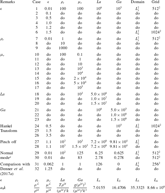
. The parametric space is large and the simulations carried out for the present study are listed in table 1. The choice for the range of values for
 $La$
and
 $Ga$
arise from the fact that for air–water combination, these numbers are very large e.g. for air as the upper fluid and water as lower fluid in the Earth’s gravitational field in CGS units,
 $T=72,\unicode[STIX]{x1D70C}\text{}^{{\mathcal{U}}}=1.5\times 10^{-3},\unicode[STIX]{x1D70C}\text{}^{{\mathcal{L}}}=1,\unicode[STIX]{x1D707}\text{}^{{\mathcal{U}}}=1.8\times 10^{-4},k=1,g=981$
leads to
 $Ga=6.81\times 10^{4}$
and
 $La=3.33\times 10^{6}$
. While most of the simulations are done with a domain size of
 $[0,7.0155]\times [0,7.0155]$
, for others (table 1) larger domains were necessary (see § 5).
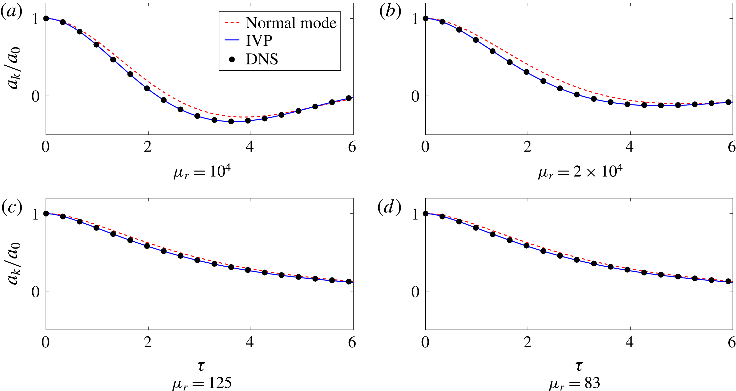
Comparisons between normal mode approximation, initial value problem and Navier–Stokes simulation for cases (a) 14, (b) 15, (c) 29 and (d) 30 in table 1.

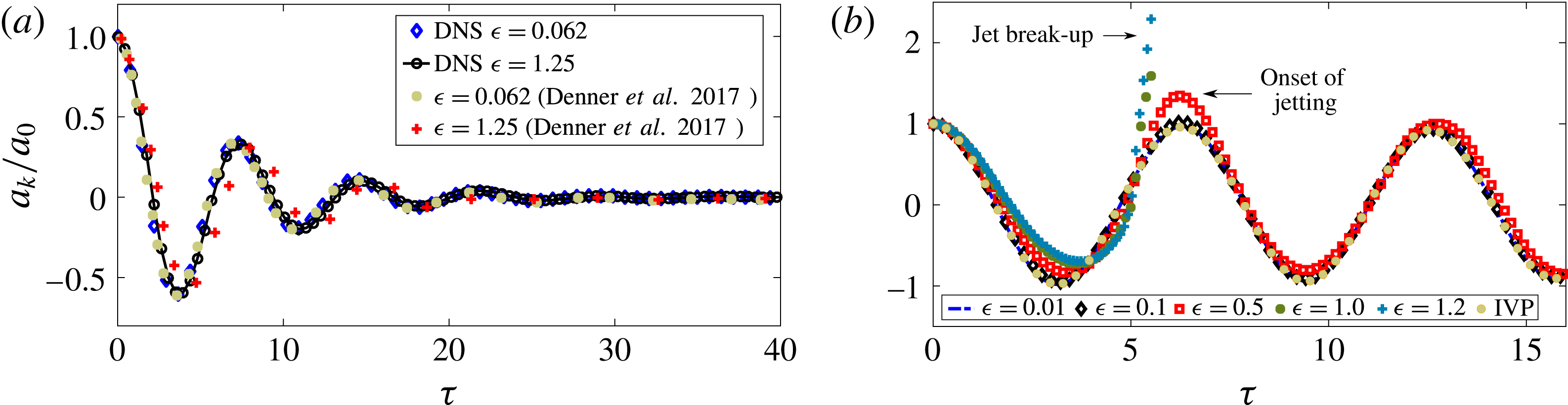
(a) Cases 31, 32 in table 1 – comparison of axisymmetric DNS simulations with planar DNS simulations of Denner et al. (Reference Denner, Paré and Zaleski2017a
) for small- and large-amplitude, pure capillary oscillations. (b) Effect of increase of
 $\unicode[STIX]{x1D716}$
for cases 1, 2, 3, 4 and 5 in table 1. Note the onset of ‘jetting’ and subsequent break-up as
 $\unicode[STIX]{x1D716}$
is increased.

DNS Parameters.

a Cases 14 and 15 are also use for normal mode comparison with DNS.
The bottom row of the table lists the simulation parameters and their formulae/values. Simulations having square domain of size
 $L_{1},L_{2},L_{3}$
and
 $L_{4}$
are performed. The values for these are in centimetres and
 $L_{1}\times L_{1}\equiv L_{1}^{2}$
etc.
5 Results and discussion
A comparison of the normal mode approximation (3.3), the IVP solution in (2.18) inverted numerically (McClure Reference McClure2016) and results from DNS are presented in figure 2. Note that
 $\unicode[STIX]{x1D70F}\equiv t\unicode[STIX]{x1D714}_{0}$
with
 $\unicode[STIX]{x1D714}_{0}^{2}\equiv gk(\unicode[STIX]{x1D70C}\text{}^{{\mathcal{L}}}-\unicode[STIX]{x1D70C}\text{}^{{\mathcal{U}}}/\unicode[STIX]{x1D70C}\text{}^{{\mathcal{L}}}+\unicode[STIX]{x1D70C}\text{}^{{\mathcal{U}}})+(Tk^{3}/\unicode[STIX]{x1D70C}\text{}^{{\mathcal{U}}}+\unicode[STIX]{x1D70C}\text{}^{{\mathcal{L}}})$
. In the case of simulations, the location of the interface is tracked at the axis of symmetry i.e.
 $r=0$
(although any other radial location also shows the same trend). Figure 2(a,b) correspond to under-damped oscillations while figure 2(c,d) are for over-damped oscillations. The excellent agreement between the solution to the IVP and the Navier–Stokes simulation is apparent. It is also seen that while normal mode is a good approximation to the IVP solution (2.20) for low values of
 $\unicode[STIX]{x1D707}_{r}$
, the difference between the two increases at higher values of viscosity ratio, especially at intermediate times. Figure 3(a) validates the analytical prediction made in § 2. For sufficiently small amplitudes, our axisymmetric DNS results agree very well with the planar DNS results obtained from Denner et al. (Reference Denner, Paré and Zaleski2017a
) (rows #42 and #113 in data provided in Denner, Paré & Zaleski (Reference Denner, Paré and Zaleski2017b
). The axisymmetric wavenumber
 $k$
of the Bessel mode was chosen to be the same as the planar wavenumber in Denner et al. (Reference Denner, Paré and Zaleski2017b
)). This comparison is done for a pure capillary wave with zero gravity. At larger amplitudes, the axisymmetric simulation shows deviations from the planar one. In agreement with the earlier observations of Denner et al. (Reference Denner, Paré and Zaleski2017a
), increasing the amplitude decreases the frequency (Prosperetti Reference Prosperetti1980) of oscillation in the axisymmetric case as well (see Becker, Hiller & Kowalewski (Reference Becker, Hiller and Kowalewski1991) and Trinh & Wang (Reference Trinh and Wang1982) for analogous observations for large-amplitude droplet oscillations). Figure 3(b) shows the effect of increasing
 $\unicode[STIX]{x1D716}$
on amplitude
 $a_{k}(t)$
as a function of time. For
 $\unicode[STIX]{x1D716}=0.01$
and
 $0.1$
, the IVP solution given by (2.20) is an excellent approximation. For
 $\unicode[STIX]{x1D716}$
larger than
 $0.5$
, there are marked deviations due to nonlinear effects. For increasing values of
 $\unicode[STIX]{x1D716}$
, the interface at the axis of symmetry starts rising to a height greater than
 $a_{k}(0)$
. We call this phenomena ‘jetting’. Note that for pure capillary waves in figure 3(a), one does not observe jetting at the non-dimensional parametric values reported in Denner et al. (Reference Denner, Paré and Zaleski2017a
). While observations of jetting (Worthington jets) have been reported earlier in the context of standing waves hitting a wall (Longuet-Higgins Reference Longuet-Higgins2001), standing waves generated through forced oscillations (Zeff et al.
Reference Zeff, Kleber, Fineberg and Lathrop2000), droplet impact (Bartolo, Josserand & Bonn Reference Bartolo, Josserand and Bonn2006) and water entry of axisymmetric objects (Gekle & Gordillo Reference Gekle and Gordillo2010), observation of jetting in purely free oscillations is reported here for the first time. In figure 3(b), as
 $\unicode[STIX]{x1D716}$
is increased further up to a value of
 $1.2$
, a droplet pinches off from the jet. This is referred to as jet break-up and droplet pinch off (see Leal (Reference Leal2007), p. 83 for discussion of a capillary mechanism of end pinch off in cylindrical threads).
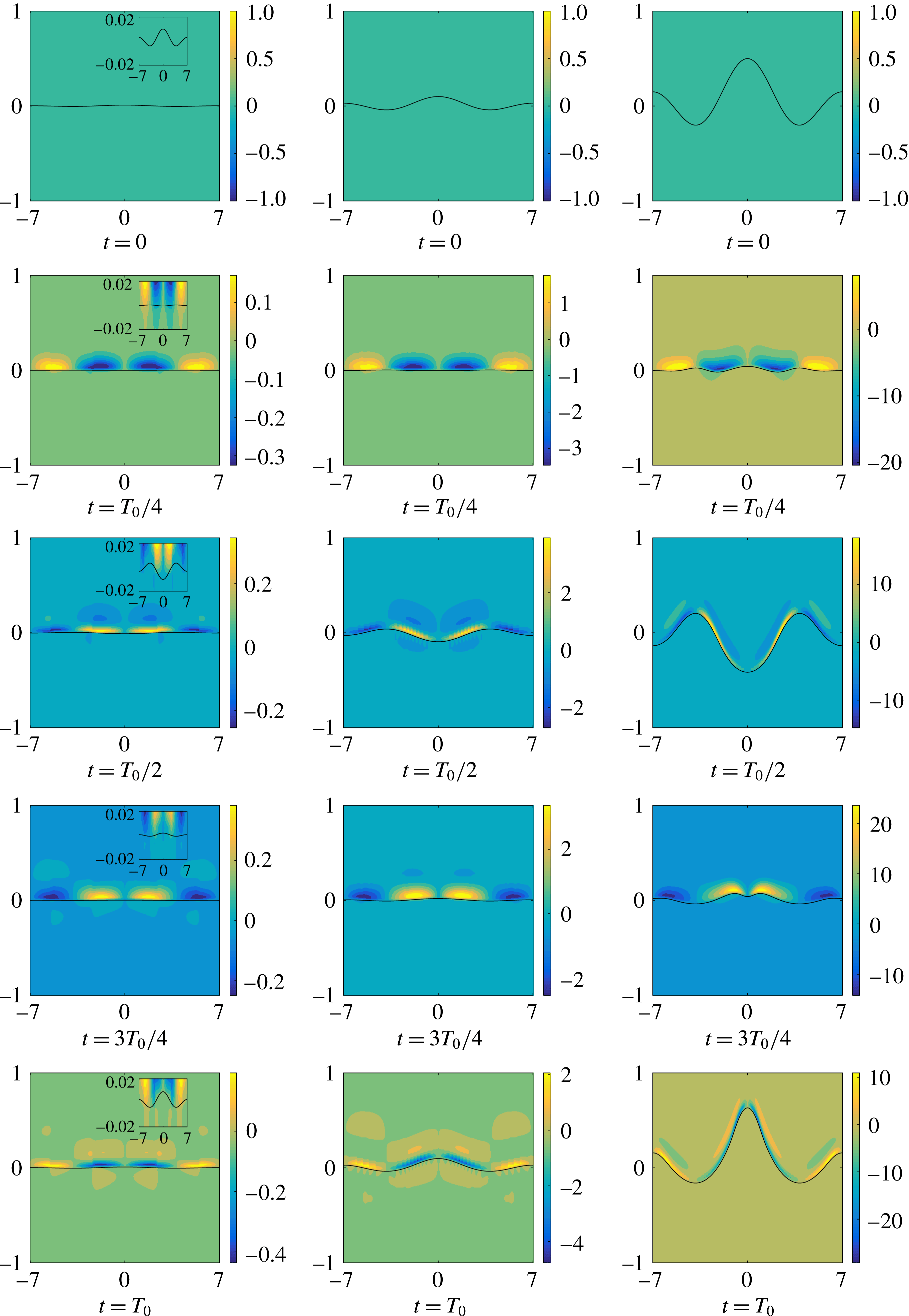
Interface with vorticity contours for cases 1, 2 and 3 in table 1. For visualisation, the interface is mirrored about the axis of symmetry. From left to right
 $\unicode[STIX]{x1D716}=0.01,0.1$
and
 $0.5$
respectively for the columns. Note the onset of ‘jetting’ in the third column.

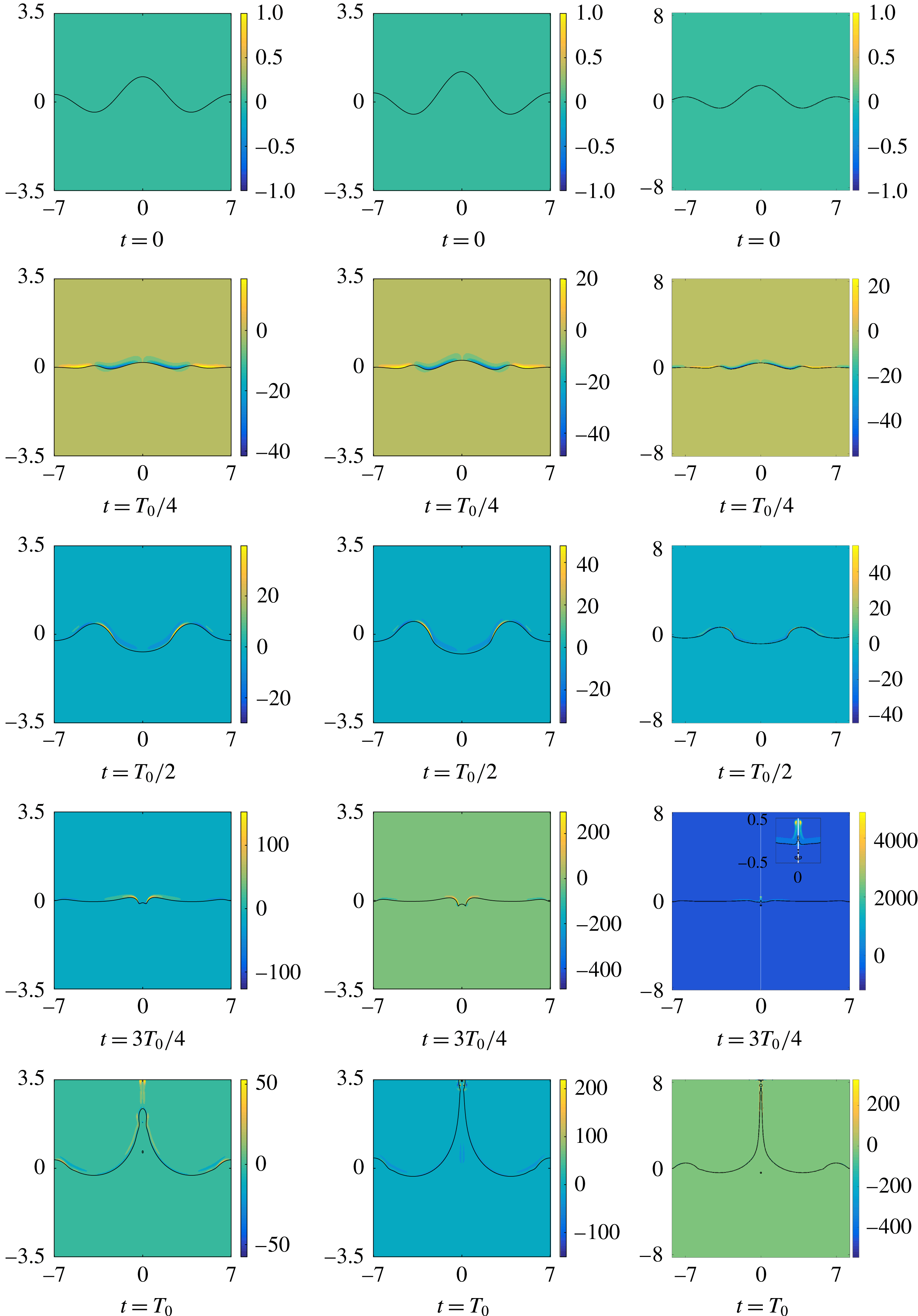
Interface with vorticity contours for cases 4, 5 and 6 in table 1. From left to right
 $\unicode[STIX]{x1D716}=1.0,1.2$
and
 $1.5$
respectively for the columns. Due to strong jetting in case of
 $\unicode[STIX]{x1D716}=1.5$
, the domain size had to be enlarged. Domain size independence of results has been verified for all cases.

The effect of increasing
 $\unicode[STIX]{x1D716}$
is visualised as a collage in figures 4 and 5. Both these figures are to be read along columns. Each column shows the interface evolving in time for a particular value of
 $\unicode[STIX]{x1D716}$
, all other non-dimensional parameters being the same. The background colour contours represent the vorticity field. It is clearly seen from figure 4 that most of the vorticity is limited to a thin region around the interface, with the maximum value of vorticity being an increasing function of
 $\unicode[STIX]{x1D716}$
. It is also seen that the peak value of vorticity (magnitude) seems to concentrate in the lighter fluid (see Tripathi, Sahu & Govindarajan (Reference Tripathi, Sahu and Govindarajan2014) and Dixit & Govindarajan (Reference Dixit and Govindarajan2010) for related analysis of this). Further the magnitude of the vorticity fields is an increasing function of
 $\unicode[STIX]{x1D716}$
as seen from the increasing scale of the colour bars. Impending droplet pinch off is clearly visible in the last image of all three columns in figure 5. For
 $\unicode[STIX]{x1D716}$
larger than
 $0.5$
, nonlinear effects are clearly visible e.g. the instantaneous shape of the interface at the row corresponding to
 $t=T_{0}/2$
(
 $T_{0}\equiv 2\unicode[STIX]{x03C0}/\unicode[STIX]{x1D714}_{0}$
) in all the columns in figure 5 is very different from
 $\text{J}_{0}(kr)$
, the assumption in (2.1). However at the end of one oscillation (for
 $\unicode[STIX]{x1D716}\leqslant 0.5$
), the interface returns to a shape which is approximately
 $\text{J}_{0}(kr)$
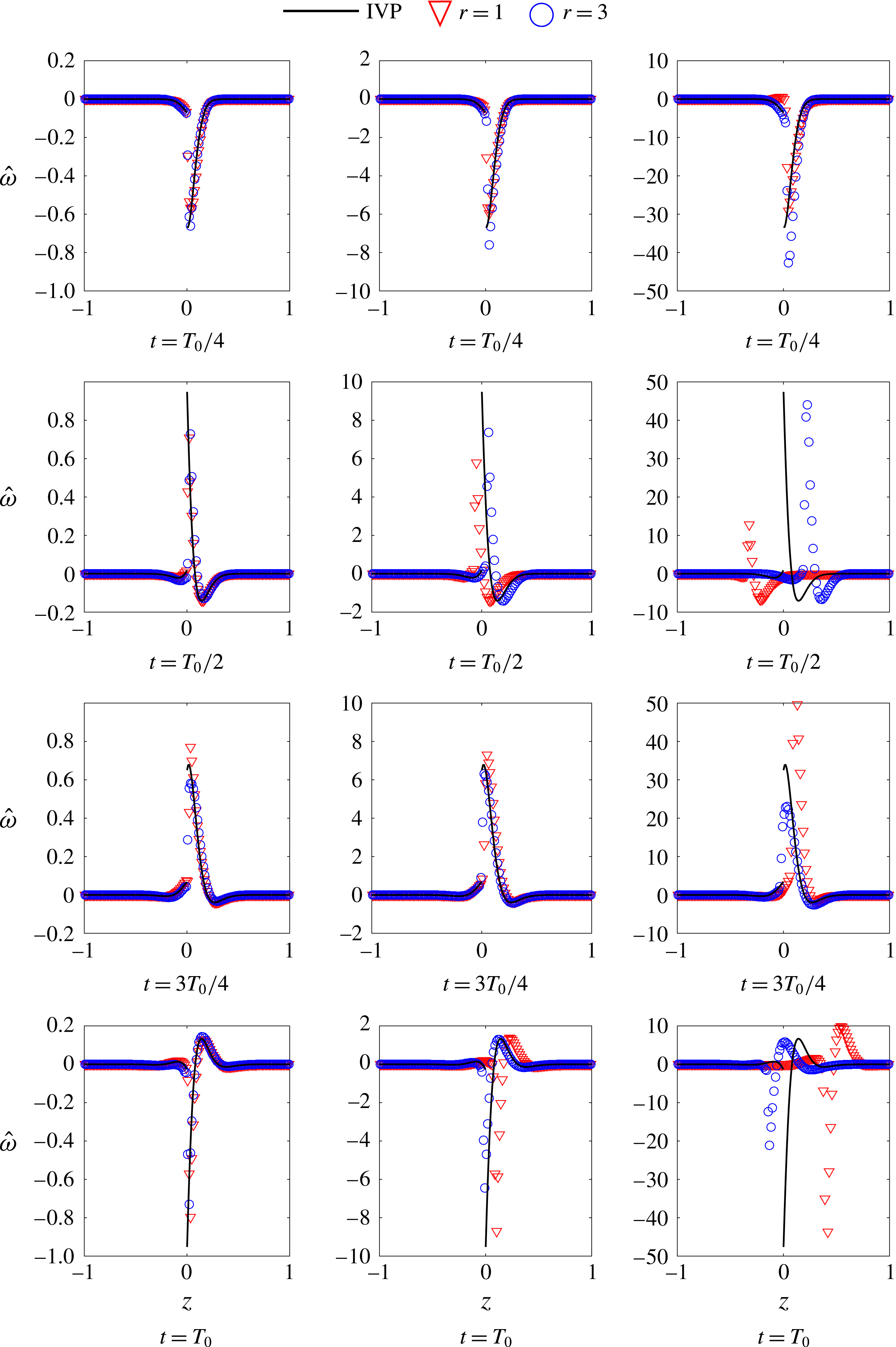
again, cf. last row of figure 4. In figure 6, we compare the IVP predictions of the vorticity field from (2.22) (see Farsoiya et al. (Reference Farsoiya, Mayya and Dasgupta2017) for the expression for the upper fluid). Equation (2.22) and the corresponding equation for the upper fluid was numerically integrated in Mathematica (Wolfram Research Inc. 2010) using the subroutine NIntegrate. Note that
 $\hat{\unicode[STIX]{x1D714}}\equiv \unicode[STIX]{x1D714}/\text{J}_{1}(kr)$
. The left column for
 $\unicode[STIX]{x1D716}=0.01$
shows excellent agreement with DNS results in both the fluids. The collapse of the curves at different radial locations
 $r=1,3$
shows the accuracy of the linear estimation. Note that the extrema of vorticity for the upper and lower fluid are slightly above and below the linearised interface
 $z=0$
. In figure 6, as
 $\unicode[STIX]{x1D716}$
is increased (
 $\unicode[STIX]{x1D716}=0.5$
), systematic deviations are seen from linear predictions. While the shapes of the vorticity profiles at different radial locations appear broadly the same, a collapse of these profiles by scaling with
 $\text{J}_{1}(kr)$
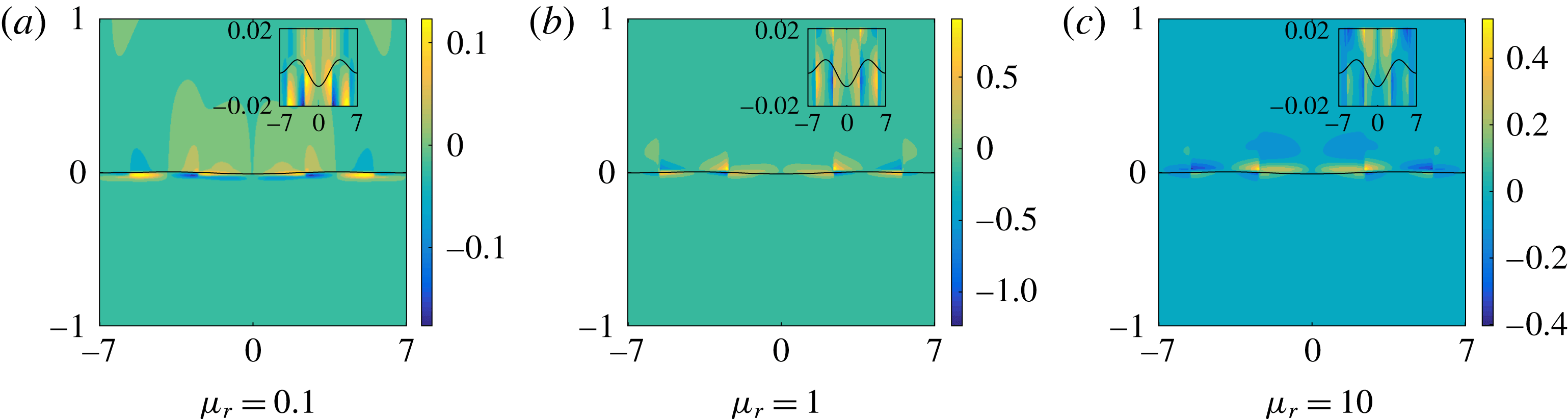
no longer appears possible, hinting at the appearance of higher modes. It is also seen that there is a vorticity jump at the interface. The inset in the first column in figure 4 shows this jump as we cross the interface. This is consistent with the linearised predictions from (2.12) reflecting the fact that the interface acts as a source of vorticity (Brøns et al.
Reference Brøns, Thompson, Leweke and Hourigan2014). The vorticity jump at the interface can however be minimised by choosing the viscosity ratio
 $\unicode[STIX]{x1D707}_{r}=1$
. To see this, we rewrite (2.12) as,
 $$\begin{eqnarray}\unicode[STIX]{x1D6FA}\text{}^{{\mathcal{U}}}(0,t)=\unicode[STIX]{x1D707}_{r}\unicode[STIX]{x1D6FA}\text{}^{{\mathcal{L}}}(0,t)-2k(\unicode[STIX]{x1D707}_{r}-1){\dot{a}}_{k}(t).\end{eqnarray}$$
It is clear that for
 $\unicode[STIX]{x1D707}_{r}=1$
, the vorticity jump between the upper and lower fluid at the interface goes to zero i.e.
 $\unicode[STIX]{x1D6FA}\text{}^{{\mathcal{L}}}(0,t)=\unicode[STIX]{x1D6FA}\text{}^{{\mathcal{U}}}(0,t)$
. This prediction is borne out by simulations. In the insets of figure 7(a–c) as we make
 $\unicode[STIX]{x1D707}_{r}=1$
(figure 7
b), the difference between the colour of vorticity contours reduces as we cross the interface, although it does not become zero. Note that (5.1) predicts that for
 $\unicode[STIX]{x1D707}_{r}\neq 1$
, the vorticity jump across the interface depends both on viscosity ratio as well as the density ratio, through
 ${\dot{a}}_{k}(t)$
. It should be remembered that (5.1) is a linearised prediction applicable to the vorticity values immediately above and below the interface only.
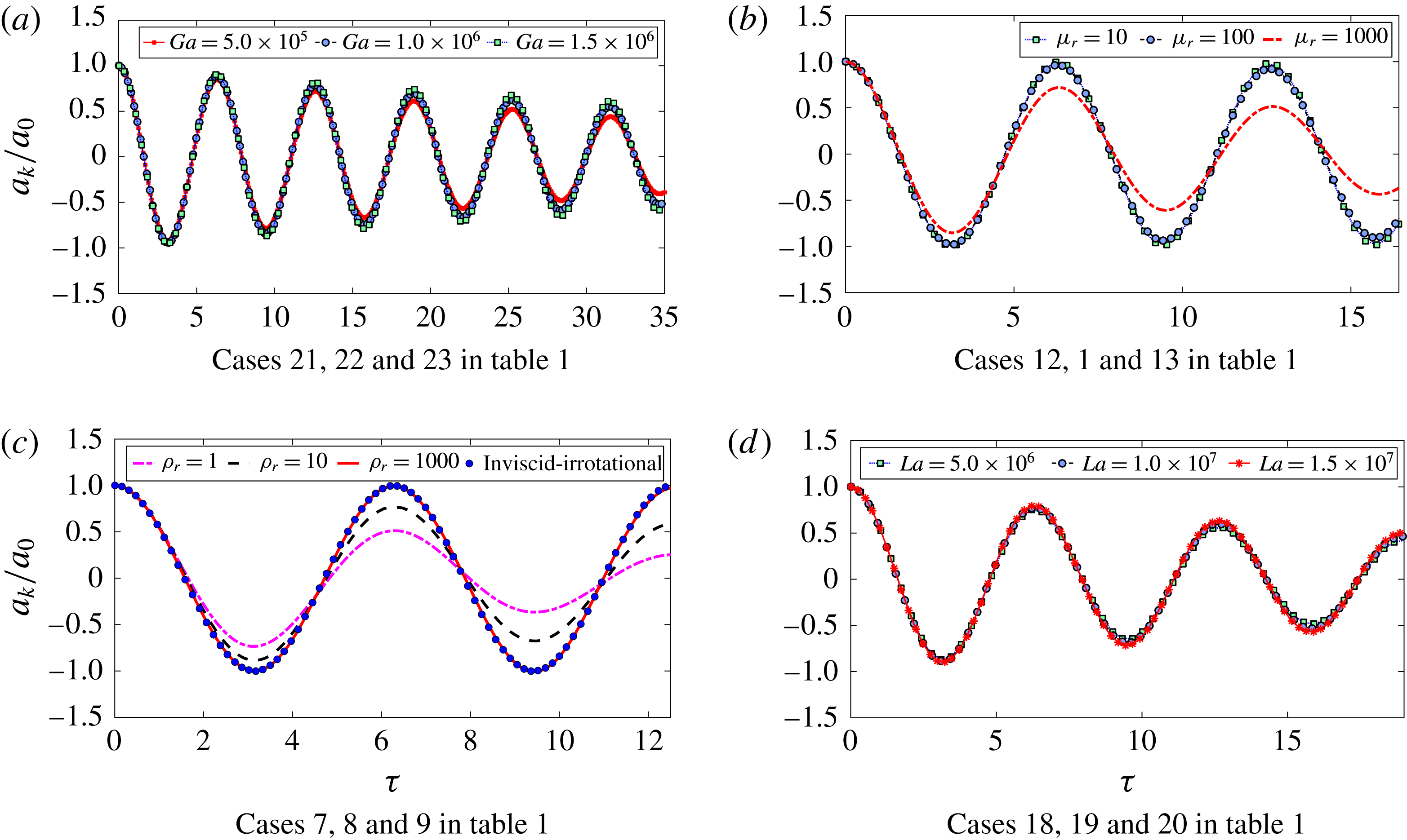
Figure 8 shows the effect of variation of parameters on under-damped oscillations. Figure 8(a) shows the influence of Galilei number. At larger values of
 $Ga$
, one can collapse all the curves by scaling
 $t$
with
 $\unicode[STIX]{x1D714}_{0}$
. However this collapse fails as one reduces the value of
 $Ga$
. Note however that for surface tension driven, pure capillary oscillations a collapse is possible using the time scale proposed in Denner (Reference Denner2016). This is demonstrated in Farsoiya et al. (Reference Farsoiya, Mayya and Dasgupta2017). Increasing the viscosity ratio in figure 8(b) increases the damping but the time period remains relatively unaffected. Increasing the density ratio in figure 8(c) has an effect both on the time period (as one can estimate from the inviscid dispersion relation) as well as on the damping. Note that for
 $\unicode[STIX]{x1D70C}_{r}=1$
, the effect of gravity drops out and these become under-damped pure capillary oscillations. For
 $\unicode[STIX]{x1D70C}_{r}=1000$
(
 $\unicode[STIX]{x1D707}_{r}=100$
), the inviscid-irrotational approximation of a undamped harmonic oscillator with frequency
 $\unicode[STIX]{x1D714}_{0}$
is an excellent approximation for the first few oscillations. The effect of change of Laplace number is shown in figure 8(d) where we see some damping but hardly any change in the time period.
Vorticity
 $\hat{\unicode[STIX]{x1D714}}\equiv \unicode[STIX]{x1D714}_{\unicode[STIX]{x1D703}}/\text{J}_{1}(kr)$
versus
 $z$
for cases 1, 2 and 3 in table 1. From left to right, the columns are for
 $\unicode[STIX]{x1D716}=0.01,0.1$
and
 $0.5$
respectively.

See inset: top–bottom vorticity asymmetry
 $\unicode[STIX]{x1D6FA}\text{}^{{\mathcal{U}}}(0,t)/\unicode[STIX]{x1D6FA}\text{}^{{\mathcal{L}}}(0,t)$
at the linearised interface
 $z=0$
changes by varying the viscosity ratio from
 $\unicode[STIX]{x1D707}_{r}<1$
through
 $\unicode[STIX]{x1D707}_{r}=1$
to
 $\unicode[STIX]{x1D707}_{r}>1$
. Cases (a) 10, (b) 11 and (c) 12.

Amplitude versus
 $\unicode[STIX]{x1D70F}$
with respect to all non-dimensional parameters.

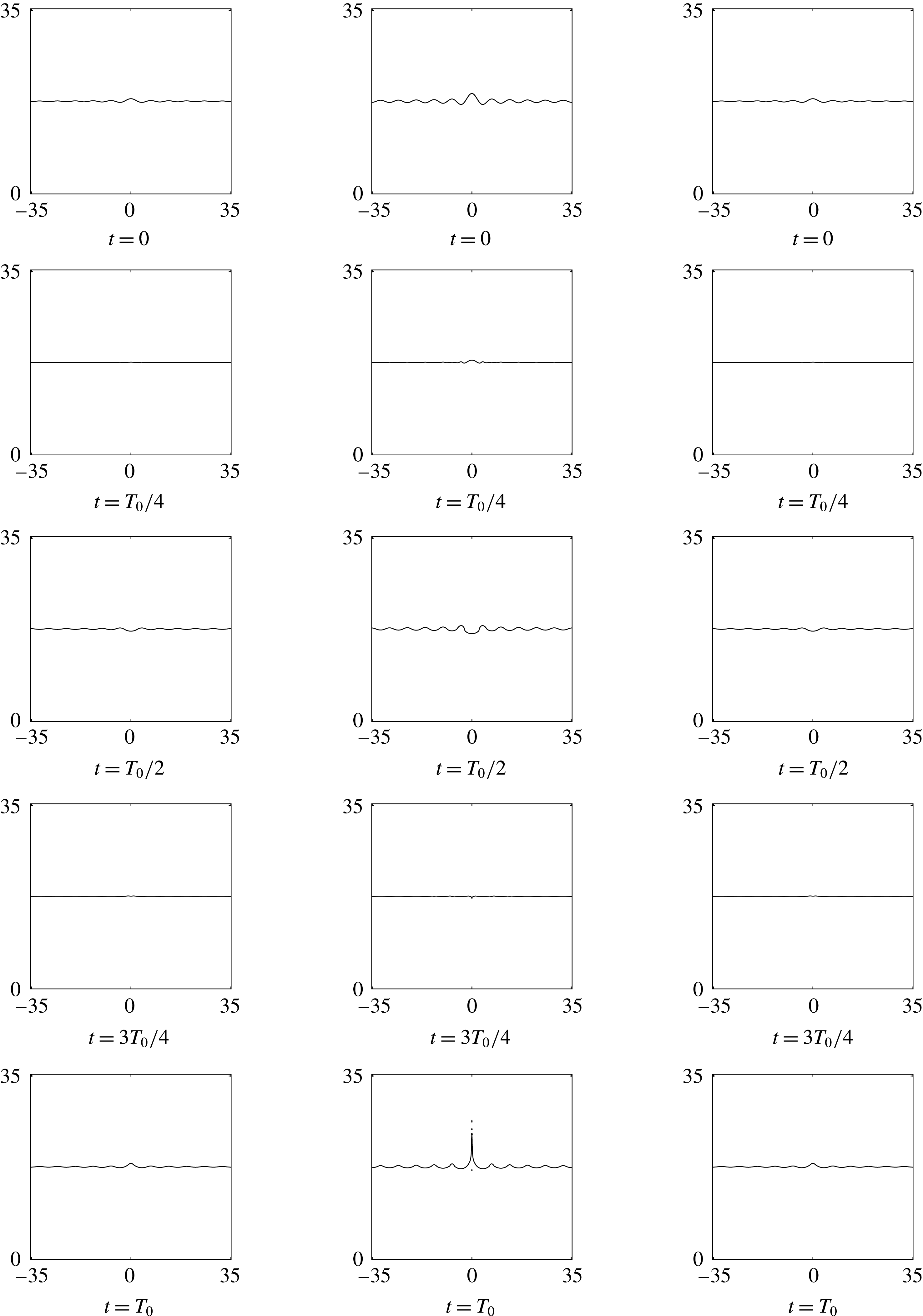
Interface for
 $\unicode[STIX]{x1D716}=0.5,1.5$
and
 $3.5$
for cases 24, 25 and 26 in table 1.


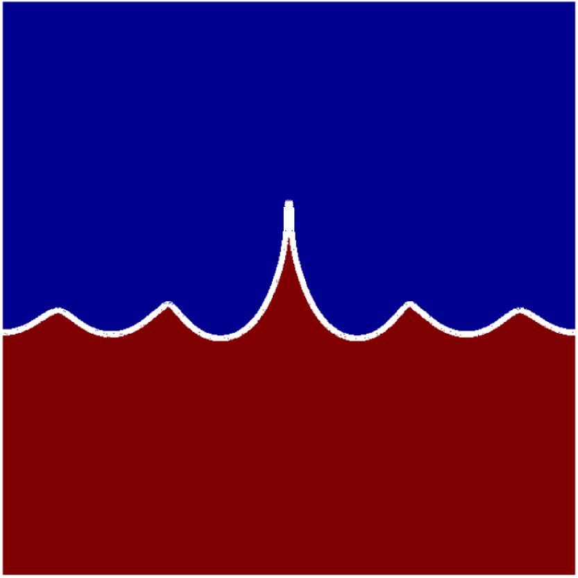
Sharp crests and rounded troughs – case 28 in table 1.

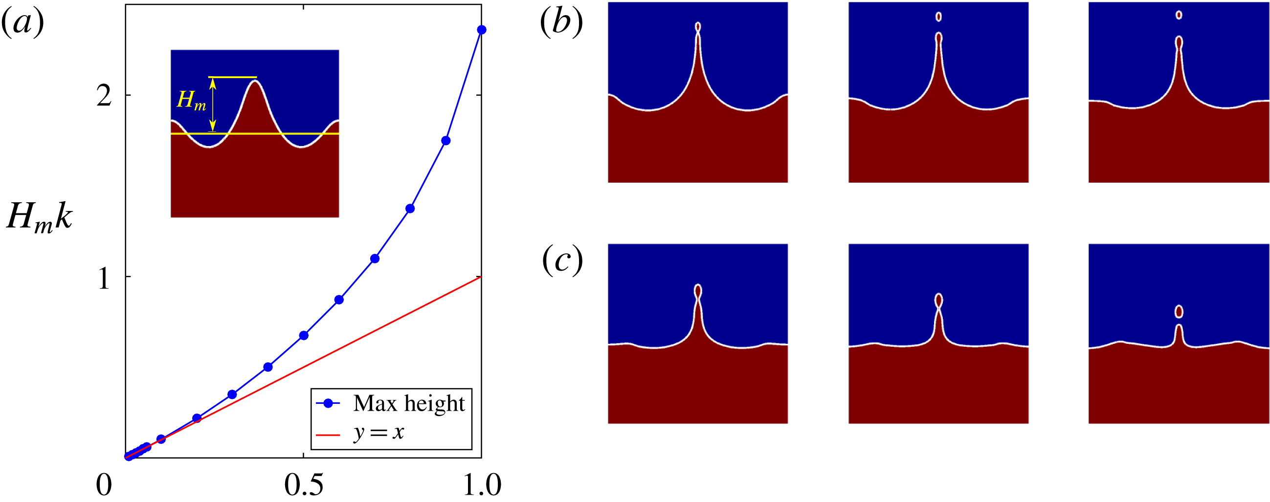
(a) Maximum jet height versus perturbation amplitude – variation of
 $H_{m}k$
with
 $\unicode[STIX]{x1D716}$
. All other parameters are for case 1 in table 1. The inset shows how
 $H_{m}$
is measured. The
 $y=x$
line is for visual reference to show the onset of jetting. (b) Droplet pinch off for an advancing jet – case 27 in table 1. (c) Pinch off in a receding jet – case 28 in table 1.

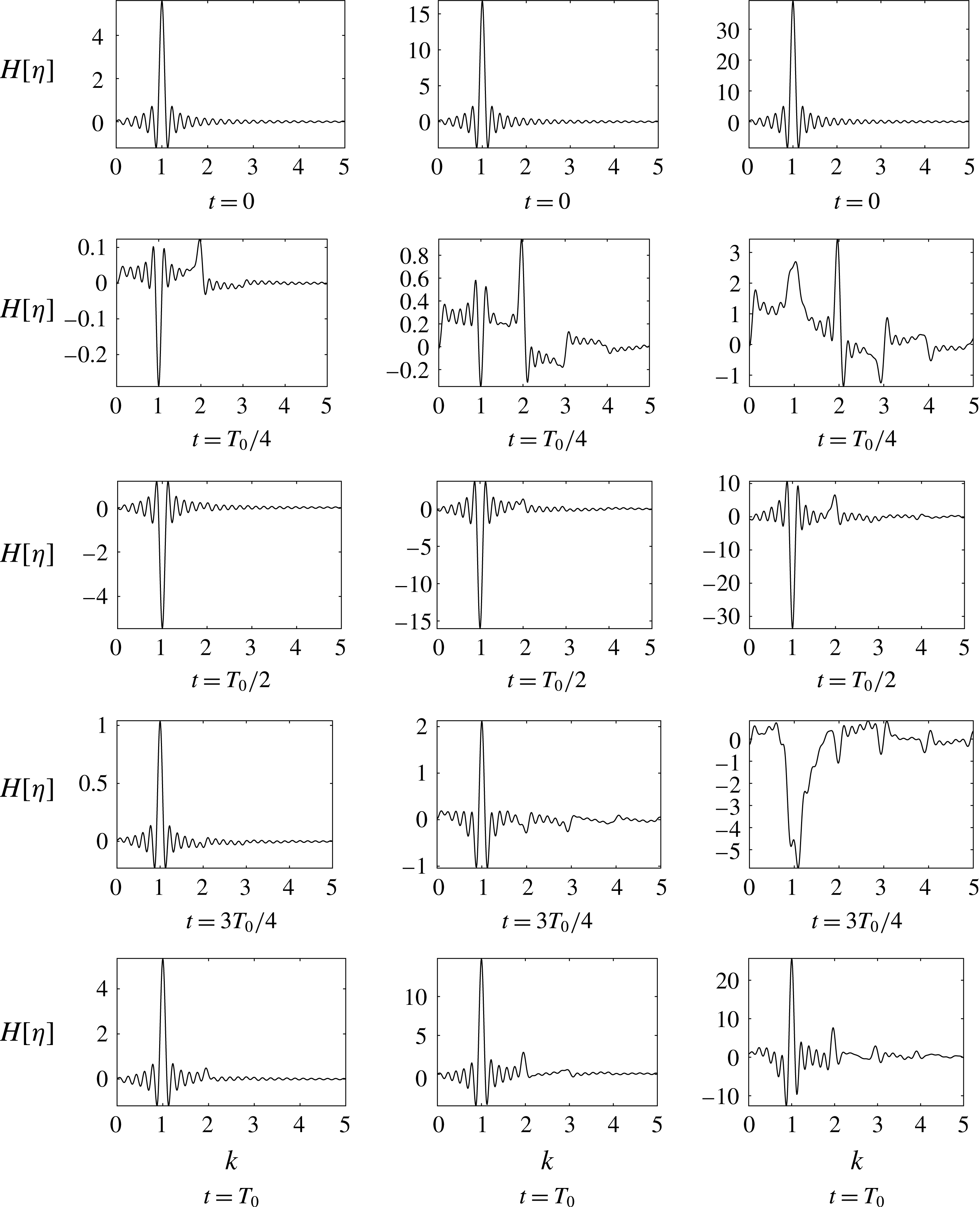
In order to understand the modal structure of the interface and study the emergence of new modes due to nonlinearity, we use Hankel transform of the interface defined by the following
 $$\begin{eqnarray}H[\unicode[STIX]{x1D702}(r,t)]=\int _{0}^{L}r\unicode[STIX]{x1D702}(r,t)\text{J}_{0}(kr)\,\text{d}r,\end{eqnarray}$$
where
 $L$
is the radial domain length used in the simulations. Hankel transform
 $H[\unicode[STIX]{x1D702}]$
is done for the interface
 $\unicode[STIX]{x1D702}(r,t)$
using an in house subroutine written in MATLAB (2015). The code was validated by reproducing the results given in Mathematica (2017) for
 $L=1000$
(
 $L\rightarrow \infty$
recovers the Hankel transform). The numerical noise in the evaluation of (5.2) reduces as
 $L\rightarrow \infty$
. As the domain size
 $[0,7.0155]\times [0,7.0155]$
produced a very noisy transform, we performed additional larger domain simulations (
 $[0,35.3323]\times [0,35.3323]$
, cases 24, 25 and 26 in table 1) for evaluating the Hankel transform. In all cases, we checked and found that the interface evolution was independent of the domain size to working precision. The interface evolution is shown in figure 9 while the corresponding Hankel transform of the interface is shown in figure 10. The columns in both figures represent
 $\unicode[STIX]{x1D716}=0.5,1.5$
and
 $3.5$
from left to right with each figure showing the interface (figure 9) and Hankel transform (figure 10) at various instants of time. It is seen that the second mode
 $k=2$
starts appearing with a magnitude comparable to
 $k=1$
for
 $\unicode[STIX]{x1D716}=1.5$
. For
 $\unicode[STIX]{x1D716}=3.5$
, the second, third and fourth modes (
 $k=2,3$
and
 $4$
) also appear. It is interesting to note that for
 $\unicode[STIX]{x1D716}$
greater than
 $0.5$
, at the end of one inviscid time period, higher modes survive along with the initial mode
 $k=1$
. Note that in figure 9 last column, the interface becomes a multivalued function of radius near
 $r=0$
. The Hankel transform for this case was obtained by excluding this small region of multivaluedness near
 $r=0$
. Figure 11, represents an instantaneous snapshot of the interface. A qualitative aspect of nonlinearity is clearly visible from the picture which shows that the crests are sharp while the troughs are rounded. This is reminiscent of cnoidal solutions of the Korteweg-de Vries equation (Dasgupta, Tomar & Govindarajan Reference Dasgupta, Tomar and Govindarajan2015). In figure 12(a), we plot the maximum height
 $H_{m}$
reached by the jet as a function of initial amplitude, when no droplet pinch off is yet observed. The inset of figure 12(a) shows the way we measure
 $H_{m}$
in our simulations i.e. when the jet has reached its maximum vertical extent. Figure 12(b) shows droplet pinch off for an advancing jet while figure 12(c) shows the same for a receding jet. The two simulations differ in their values of viscosity ratio
 $\unicode[STIX]{x1D707}_{r}$
only.
6 Conclusions and future work
In this study, we have solved the linearised IVP of an axisymmetric perturbation initialised as a Bessel mode on the interface of two radially unbounded, viscous immiscible fluids. We find that a small-amplitude Bessel mode evolves temporally in the same way as a spatial Fourier mode in planar geometry. We compare our analytical results to the normal mode approximation and to DNS. For small amplitudes, the DNS results compare extremely well to the solution of the IVP. The normal mode approximation is found to be good at very early and late times with deviations at intermediate times. The vorticity jump across the interface is found to depend in general both on the density and viscosity ratios of the two fluids. We show that by choosing the viscosity ratio to be unity, the magnitude of this jump can be reduced. Upon increasing the initial amplitude of perturbation, nonlinear effects produce qualitatively new features not present in the linearised IVP solution. Notable among these is the formation of a jet at the axis of symmetry which can rise to a height much greater than the parent perturbation. Depending on the viscosity ratio, the jet may undergo end pinch off while advancing or receding, leading to daughter droplet formation. A relation between the maximum jet height and the initial perturbation amplitude is obtained. Parametric studies are reported for the effect of change of parameters on under-damped oscillations. The emergence of new modes is studied using the Hankel transform of the interface.
The results obtained in this study will be useful in varied contexts. The analytical formulae presented here for
 $a_{k}(t),p_{v}(r,z,t)$
and
 $\unicode[STIX]{x1D714}_{\unicode[STIX]{x1D703}}(r,z,t)$
are useful for benchmarking codes. From a more fundamental perspective, our analytical results for a single Bessel mode can be used to solve the axisymmetric Cauchy–Poisson problem (for arbitrary initial conditions) in closed form, taking into account viscosity and inertia in both the fluids. For general initial conditions which excite a large (an uncountable infinite) number of modes at
 $t=0$
, one would expect deviations from predictions made by the normal mode approximation when compared to IVP predictions. A comparison of the contribution of the continuous spectrum modes vis-a-vis discrete normal modes for general initial conditions, requires more simulations and analysis. This is currently underway and will be presented in a forthcoming publication. The study of jetting and subsequent droplet pinch off and the role of interfacial vorticity in these, will help obtain better and more detailed understanding of droplet impact on a deep pool. Finally, the linearised, unsteady, base state solution presented here will find applications in the study of forced oscillations like Faraday waves.
Acknowledgements
R.D. and P.K.F. acknowledge Industrial Research and Consultancy Centre (IRCC), IIT Bombay for a start up grant and for supporting the latter’s PhD fellowship. We thank Science and Engineering Research Board (SERB), Dept. of Science and Technology, Govt. of India (grant no. EMR/2016/000830) for financial support for a related study of interfacial oscillations. R.D. acknowledges a useful discussion with R. Govindarajan on vorticity asymmetry across an interface.
Supplementary data
Supplementary data is available at https://doi.org/10.1017/jfm.2017.443.