


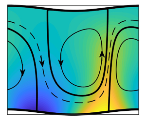





1. Introduction
Several external mechanisms can influence the motion of a convective fluid within a channel. If the sides of the channel are not flat, any topography may cause the fluid to move; furthermore, a temperature distribution applied to one or both sides of the channel may affect the flow. Thermal drift is the motion produced by combining a grooved geometry of the boundaries and an imposed heating pattern (Abtahi & Floryan Reference Abtahi and Floryan2017a; Floryan & Inasawa Reference Floryan and Inasawa2021; Inasawa, Hara & Floryan Reference Inasawa, Hara and Floryan2021). If the heating profile is periodic, the consequent convection appears as counter-rotating rolls with a spatial structure dictated by the heating wavenumber. The associated pressure field projects onto the geometry of the grooves and produces a force that drives a net flow along the channel. The magnitude and direction of this flow depend on the relative positions of the heating and groove patterns, and even though the applied heating is periodic, the convection generates a net heat flow across the slot (Abtahi & Floryan Reference Abtahi and Floryan2017b). The drift is generated irrespective of the heating intensity, so this effect is essentially a forced system response rather than any form of bifurcation. The mechanism of thermal drift can be used for several processes including fluid pumping (Floryan, Haq & Panday Reference Floryan, Haq and Panday2022) or propulsion (Floryan, Aman & Panday Reference Floryan, Aman and Panday2024a). It should be emphasized that there is a slightly subtle difference between thermal drift and thermal streaming, as the latter requires a sufficiently strong heating intensity (Floryan, Panday & Aman Reference Floryan, Panday and Aman2023). Periodic heating may yield a propulsive effect via streaming, but only if the spatial distribution is appropriately chosen and the heating is sufficiently strong; in this regard, streaming is the upshot of a bifurcation behaviour (cf. the earlier remarks regarding thermal drift).
Any analysis of the interaction of the two types of flow actuation (i.e. the boundary topography and the heating pattern) requires an appropriate specification of these distributions. For general periodic patterns, the forcing clearly ought to be written in the form of a Fourier series. Except for very special situations, the solution for the subsequent flow structure can then only be determined using fully numerical simulations. One drawback of this approach is that it can be difficult to appreciate the important facets of the underpinning mechanisms. Here, we adopt an alternative strategy and suppose that a single Fourier mode describes both the channel geometry and the imposed heating. While this may seem somewhat over-simplistic, we point out that in some previous studies (Floryan Reference Floryan2007), it has been found that if a single Fourier component is used to approximate a complicated geometry, the corresponding flow properties can often accurately capture the main features of the system response. This is sometimes referred to as a reduced geometry model but perhaps can be considered more generally as a reduced distribution mode. This device neatly sidesteps the need to study numerous separate cases, as their properties can be reliably estimated using the reduced model. We shall demonstrate later that reduced distribution models can legitimately be used to study the interaction of topography and temperature patterns.
It has been established that spatially patterned heating alone can reduce the pressure losses observed in channel flows (Hossain, Floryan & Floryan Reference Hossain, Floryan and Floryan2012; Floryan & Floryan Reference Floryan and Floryan2015; Hossain & Floryan Reference Hossain and Floryan2016; Inasawa, Taneda & Floryan Reference Inasawa, Taneda and Floryan2019). When combined with a groove structure, a larger reduction is achievable if the relative positions of the grooves and the heating are properly selected (Floryan, Shadman & Hossain Reference Floryan, Shadman and Hossain2018; Hossain & Floryan Reference Hossain and Floryan2020; Floryan, Aman & Panday Reference Floryan, Aman and Panday2024b). The reason for these reductions can be traced to the properties of convection rolls present in the flow. The upshot is that pressure reductions are only achievable when the flow is relatively modest; if it is too strong, it completely washes the rolls away and the potential for pressure reduction is lost. In practical terms, no resistance reduction can occur once the Reynolds number exceeds approximately 100. Moreover, it should be remarked that periodic heating may induce instabilities in a horizontal fluid layer driven by the spatial parametric resonance (Hossain & Floryan Reference Hossain and Floryan2013, Reference Hossain and Floryan2015, Reference Hossain and Floryan2022); the mechanism underpinning this is distinct from the Rayleigh–Bénard instability (Bénard Reference Bénard1900; Rayleigh Reference Rayleigh1916; Drazin & Reid Reference Drazin and Reid2004).
Features of fluid pumping have also been observed in other contexts. In this regard, we mention that the effect can be achieved using the difference in radiative effects induced by surfaces of different colours. This process is of particular interest within the field of rarified gas dynamics (Crookes Reference Crookes1874). This concept has been utilized in conduits subject to patterns of spatial heat fluxes combined with a pattern of surface grooves, known as the ratchet effect (Shahabi et al. Reference Shahabi, Baier, Roohi and Hardt2017; Lotfian & Roohi Reference Lotfian and Roohi2019). The main driver in producing an axial pumping force is a break in the axial symmetry within the flow. Most existing analyses seem to involve a series of case studies with a wider generalized picture that is still somewhat obscure. Nevertheless, it has been shown that relatively large temperature differences are required; the interested reader is directed to the excellent review by Lotfian & Roohi (Reference Lotfian and Roohi2019) for a comprehensive review of this field.
There has been relatively little previous work that directly addresses thermal drift. Of what has been done, most of the analysis has focused on problems in which only one side of the channel is grooved while the other edge is perfectly flat. When subjected to a heating pattern, such a configuration can be thought of as forming a so-called ‘thermal drift engine’ (hereafter referred to as a TDE). One of the main issues tackled in the present work is understanding the system response when multiple patterns are used, i.e. when multiple TDEs are present. Potentially, these TDEs may either reinforce or oppose each other. We tackle this issue by allowing both sides of the channel to be grooved so that we have the possibility of interplay between two geometrical and one thermal patterns. It is far from clear at the outset whether the introduction of the third distribution will have only minimal and inconsequential implications for the flow field or whether more substantial modifications may arise. This is the central question that the remainder of this paper seeks to answer.
In the simplest case, the spatial distributions of flow actuations are characterized by three wavenumbers, with one for each of the surface topographies and temperature. Depending on the selection of these wavenumbers, the resulting flow may have various commensurate (periodic) and incommensurate (aperiodic) states (Seneta Reference Seneta1976; Laczkovich & Revesz Reference Laczkovich and Revesz1990; Keleti Reference Keleti1997; Hu Reference Hu, Wang and Chung2013). The appearance of incommensurate states has been recently recognized in hydrodynamic stability problems involving analysis of the stability of spatially modulated flows (Panday & Floryan Reference Panday and Floryan2023). In this work, we consider all patterns being characterized by the same wavenumber and focus on the effects of different relative positions of these patterns.
To this end, the remainder of the presentation is organized as follows. In § 2, we formulate the model problem: a horizontal slot bounded by plates with sinusoidal grooves. The lower plate is exposed to a heating pattern, which is also of sinusoidal form, so it has the form of a reduced distribution model. We adopt simple sinusoidal patterns since this facilitates the identification of the main mechanisms responsible for the drift. Appreciating the various processes at work is somewhat difficult to disentangle should more complicated grooves and/or heating structures be chosen. Both the upper and lower grooves activate two distinct TDEs and provide a vehicle for analysing a more involved flow driven by multiple engines (or multiple pattern interaction effects).
Section 3 focuses on the flow produced by a single engine. Although the properties of single engines are well known, it is helpful to set out the key properties before we introduce the second engine; this is done in § 4. Sections 5 and 6 provide some asymptotic justification for our findings. Section 5 examines the problem in an appropriate long-wavelength limit, while § 6 discusses a weak convection case. We derive an expression for the fluid flux and demonstrate that the result appears to be accurate for a range of parameters far wider than might have been expected. Section 7 discusses the effects of uniform heating, while § 8 comments on the effects of the Prandtl number. Section 9 suggests modifying our basic problem, which involves grooves composed of straight isothermal segments. Such a device can be readily manufactured for experiments or applications in passive horizontal pumping and provides some insight into the usefulness of adopting simplified geometry based on a single Fourier mode. The paper closes with a few final remarks.
2. Problem formulation
Consider an infinite horizontal slot formed by two corrugated plates as sketched in figure 1. We introduce the coordinate axes so that the x-axis is directed from left to right, and the positive y-axis points upwards. The geometry of the slot is then specified as
 \begin{equation}{y_L}(x) ={-} 1 + {\textstyle{1 \over 2}}{A_L}\,\textrm{cos}\,\alpha x,\quad {y_U}(x) = 1 - {\textstyle{1 \over 2}}{A_U}\,\textrm{cos(}\alpha x + {\varOmega _C}),\end{equation}
where the subscripts U and L refer to the upper and lower plates, respectively, and lengths have been made dimensionless based on the half mean slot opening h. In a practical experiment, the topographies of the surfaces might likely be somewhat intricate, but here, we model them using appropriate leading-order Fourier components. We shall revisit the question as to the accuracy of using a reduced model to describe the performance of arbitrary topographies in § 9. Both the lower and upper plates are supposed to be corrugated, and the grooves have peak-to-trough amplitudes  ${A_L}$ and
 ${A_U}$, respectively. The oscillations in the groove shape are of wavenumber
 $\alpha $ (or of wavelength
 $\lambda = 2{\rm \pi} /\alpha $) and are offset by a relative phase shift
 ${\varOmega _C}$. Changing the value of
 ${\varOmega _C}$ adjusts the geometry of the slot; the largest possible slot opening is
 $2 + {\textstyle{1 \over 2}}{A_L} + {\textstyle{1 \over 2}}{A_U}$ while the smallest opening
 $2 - {\textstyle{1 \over 2}}{A_L} - {\textstyle{1 \over 2}}{A_U}$.
A schematic of the flow system. The slot occupies the region  ${y_L}(x) \le y \le {y_U}(x)$ with the limits defined by (2.1). The temperature of the lower edge
 $y = {y_L}(x)$ is defined by (2.2a). The heating and groove oscillations are of wavenumber
 $\alpha$; the phases
 ${\varOmega _C}$ and
 ${\varOmega _{TL}}$ govern the offsets between the positions of the two boundaries and between the locations of the slots and applied heating.

The lower plate is heated, resulting in a periodic temperature profile, while the upper plate is kept isothermal. This implies that the plates’ temperature distributions are given by
 \begin{equation}{\theta _L}(x) = R{a_{uni}} + {\textstyle{1 \over 2}}R{a_{p,L}}\,\textrm{cos}(\alpha x + {\varOmega _{TL}})\quad \textrm{and}\quad {\theta _U}(x) = 0,\end{equation}
where  $\theta $ denotes the dimensionless temperature and (2.2a) consists of a single Fourier mode. This temperature is defined to be
 $\theta = T - {T_U}$ where the temperature of the upper plate
 ${T_U}$ is used as a reference level, and
 $\theta $ has been scaled on
 $\kappa \nu /(g\varGamma {h^3})$; here, g stands for the gravitational acceleration,
 $\varGamma $ is the thermal expansion coefficient,
 $\nu $ denotes the kinematic viscosity and
 $\kappa $ stands for the thermal diffusivity. We emphasize that the inclusion of the phase angle
 ${\varOmega _{TL}}$ allows us to examine the effect of varying the offset between the heating pattern and the geometry of the bottom groove. The periodic Rayleigh number
 $R{a_{p,L}}$ sets the amplitude of temperature variations of the lower boundary of the slot while the uniform Rayleigh number
 $R{a_{uni}}$ sets the intensity of the uniform heating component.
We intend to examine how the interaction between the groove and heating patterns can produce a net horizontal flow rate Q. To address this issue, we need to solve for the two-dimensional convection of Boussinesq fluid within the slot. This is governed by the continuity, Navier–Stokes, and energy equations, which we write in the form
 \begin{gather}\frac{{\partial u}}{{\partial x}} + \frac{{\partial v}}{{\partial y}} = 0,\quad u\frac{{\partial u}}{{\partial x}} + v\frac{{\partial u}}{{\partial y}} ={-} \frac{{\partial p}}{{\partial x}} + {\nabla ^2}u,\end{gather}
 \begin{gather}u\frac{{\partial v}}{{\partial x}} + v\frac{{\partial v}}{{\partial y}} ={-} \frac{{\partial p}}{{\partial y}} + {\nabla ^2}v + P{r^{ - 1}}\theta ,\quad u\frac{{\partial \theta }}{{\partial x}} + v\frac{{\partial \theta }}{{\partial y}} = P{r^{ - 1}}{\nabla ^2}\theta .\end{gather}
In this system ( $u,v$) denotes the velocity components in the (x, y) directions, respectively, scaled with
 ${U_v} = \nu /h$, while p is the pressure relative to the hydrostatic component and scaled on
 $\rho U_\nu ^2$. The parameter
 $Pr = \nu /\kappa $ is the Prandtl number, and in most of our subsequent computations, we take Pr = 0.71 (the value appropriate to air). In the derivation of the system (2.3), we have implemented the Boussinesq approximation; this is a fairly standard procedure, but a discussion of the precise circumstances under which it is appropriate has been given by Tritton (Reference Tritton1977). The results of experiments under thermal conditions similar to those used in the present analysis (Inasawa et al. Reference Inasawa, Taneda and Floryan2019, Reference Inasawa, Hara and Floryan2021; Floryan & Inasawa Reference Floryan and Inasawa2021) demonstrate that the Boussinesq approximation describes the fluid response very well.
Equations (2.3) need to be supplemented by flow and temperature conditions. We impose the no-slip, no-penetration and temperature conditions on the sides of the slot so that
 \begin{align} u(x,{y_L}) = u(x,{y_U}) = 0,\quad v(x,{y_L}) = v(x,{y_U}) = 0,\nonumber\\ \theta (x,{y_L}) = {\theta _L}(x),\qquad\quad\ \ \ \theta (x,{y_U}) = {\theta _U}(x) = 0, \end{align}
where  ${y_L}$ and
 ${y_U}$ are defined in (2.1), and the temperature profile
 ${\theta _L}(x)$ is given by (2.2a). The solution should be periodic in x (with the periodicity dictated by the heating and groove patterns), eliminating the need for boundary conditions in the x-direction. We wish to study the pumping effect resulting from pattern interactions and, thus, we eliminate any external pressure gradient, which leads to the pressure gradient constraint of the form
 \begin{equation}{\left. {\frac{{\partial p}}{{\partial x}}} \right|_{mean}} = 0.\end{equation}
The velocity components are expressed using the streamfunction  $\psi $ defined as
 ${u = \partial \psi /\partial y}$ and
 $v ={-} \partial \psi /\partial x$, and the pressure is eliminated between (2.3b,c), thereby giving the vorticity equation which is fourth order in
 $\psi $. The unknowns are expressed as Fourier expansions in the x-direction, with the modal functions expressed in terms of Chebyshev expansions in the y-direction. This form of discretization ensures that x-periodicity conditions are automatically satisfied.
The analysis of flow physics requires solutions for flow equations in a wide range of irregular domains that can arise from variations in groove wavenumbers and amplitudes. The variability of the geometry represents the main computational challenge. Typical solution strategies involve numerical grid generation, which has to be repeated with each change of the slot geometry. The immersed boundary conditions method provides better geometric flexibility and was selected for this study. The main idea of this method is to use a regular computational domain with the slot immersed in its interior. The form of the discretized flow equations remains the same for all geometries. The classical boundary conditions are replaced by the constraints (Szumbarski & Floryan Reference Szumbarski and Floryan1999; Husain & Floryan Reference Husain and Floryan2008, Reference Husain and Floryan2010; Husain, Szumbarski & Floryan Reference Husain, Szumbarski and Floryan2009), which are included using the  $\tau $-method (Canuto et al. Reference Canuto, Hussaini, Quarteroni and Zang1992) and need to be changed as geometry changes. The groove shape is encoded within the algorithm using appropriate Fourier expansions with changes in the expansion coefficients accounting for variations of the slot geometry. This method bypasses the need for numerical grid construction and omits the need for grid convergence studies. All the elements of the discretization have spectral accuracy. Global accuracy is controlled by selecting the number of Fourier modes and Chebyshev polynomials. All reported results are at least four digits. Details of this of this algorithm are presented in Panday & Floryan (Reference Panday and Floryan2021).
The net horizontal flow rate Q defined as
 \begin{equation}Q = \int_{{y_L}(x)}^{{y_U}(x)} {u(x,y)\,\textrm{d}y} \end{equation}
is determined during the postprocessing phase; Q defines the Reynolds number based on the mean horizontal velocity  ${U_m}$, i.e.
 $Re = {U_m}h/\nu = Q$.
The flow mechanics are most conveniently explained by analysing forces acting on the fluid at the bounding plates. The stress vector  ${\boldsymbol{\sigma }_L}$ at the lower plate takes the form
 \begin{equation}{\boldsymbol{\sigma }_L} = [{\sigma _{x,L}}\quad {\sigma _{y,L}}] = [{n_{x,L}}\quad {n_{y,L}}] {\left[ {\begin{array}{@{}ll@{}} {2\dfrac{{\partial u}}{{\partial x}} - p}&{\dfrac{{\partial u}}{{\partial y}} + \dfrac{{\partial v}}{{\partial x}}}\\ {\dfrac{{\partial u}}{{\partial y}} + \dfrac{{\partial v}}{{\partial x}}}&{2\dfrac{{\partial v}}{{\partial y}} - p} \end{array}} \right]_{y = {y_L}}},\end{equation}
where the normal unit vector  ${\boldsymbol{n}_L}$ pointing outwards can be expressed as
 \begin{equation}{\boldsymbol{n}_L} = [{n_{x,L}}\quad {n_{y,L}}] = {N_L}\left( {\frac{{\partial {y_L}}}{{\partial x}}, - 1} \right),\quad {N_L} = {\biggl[{1 + {{\biggl( {\frac{{\partial {y_L}}}{{\partial x}}} \biggr)}^2}} \biggr]^{ - 1/2}}.\end{equation}
The x-component of the stress vector is written as
 \begin{equation}{\sigma _{x,L}} = {\sigma _{xv,L}} + {\sigma _{xp,L}} = {N_L}\biggl[{2\frac{{\partial {y_L}}}{{\partial x}}{{\left. {\frac{{\partial u}}{{\partial x}}} \right|}_{{y_L}}} - {{\left. {\biggl( {\frac{{\partial u}}{{\partial y}} + \frac{{\partial v}}{{\partial x}}} \biggr)} \right|}_{{y_L}}}} \biggr] - {N_L}{\left. {\frac{{\partial {y_L}}}{{\partial x}}p} \right|_{{y_L}}},\end{equation}
where  ${\sigma _{xv,L}}$ and
 ${\sigma _{xp,L}}$ denote the viscous and pressure components, respectively. The x-component of the total force
 ${F_{x,L}}$ (per unit length and unit width of the slot) is expressed as
 \begin{align}{F_{x,L}} &= {F_{xv,L}} +{F_{xp,L}} = {\lambda ^{ - 1}}\int_{{x_0}}^{{x_0} + \lambda} {\biggl[ {2\frac{{\partial {y_L}}}{{\partial x}}{{\left. {\frac{{\partial u}}{{\partial x}}} \right|}_{{y_L}}} - {{\left. {\biggl( {\frac{{\partial u}}{{\partial y}} + \frac{{\partial v}}{{\partial x}}} \biggr)} \right|}_{{y_L}}}} \biggr]\textrm{d}\kern0.07em x}\nonumber\\ &\quad - {\lambda ^{ - 1}}\int_{{x_0}}^{{x_0} + \lambda } {\frac{{\partial {y_L}}}{{\partial x}}p{|_{{y_L}}}\,\textrm{d}\kern0.07em x}, \end{align}
where  ${x_0}$ is a reference point,
 ${F_{xp,L}}$ denotes the pressure force while
 ${F_{xv,L}}$ stands for the viscous force. A similar process applied to the upper plate yields
 \begin{gather}{\boldsymbol{n}_U} = [{n_{x,U}}\quad {n_{y,U}}] = {N_U}\left( { - \frac{{\partial {y_U}}}{{\partial x}},1} \right),\quad {N_U} = {\biggl[ {1 + {{\biggl( {\frac{{\partial {y_U}}}{{\partial x}}} \biggr)}^2}} \biggr]^{ -1/2}},\end{gather}
 \begin{gather}
{\sigma _{x,U}} = {\sigma
_{xv,U}} + {\sigma _{xp,U}} = {N_U}\biggl[ { -
2\frac{{\partial {y_U}}}{{\partial x}}{{\left.
{\frac{{\partial u}}{{\partial x}}} \right|}_{{y_U}}} +
{{\left. {\biggl( {\frac{{\partial u}}{{\partial y}} +
\frac{{\partial v}}{{\partial x}}} \biggr)}
\right|}_{{y_U}}}} \biggr] + {N_U}{\left. {\frac{{\partial
{y_U}}}{{\partial x}}p}
\right|_{{y_U}}},\end{gather}
 \begin{gather}{F_{x,U}} = {F_{xv,U}} +
{F_{xp,U}} = {\lambda ^{ - 1}}\int_{{x_0}}^{{x_0} + \lambda
} {\biggl[ { - 2\frac{{\partial {y_U}}}{{\partial
x}}{{\left. {\frac{{\partial u}}{{\partial x}}}
\right|}_{{y_U}}} + {{\left. {\biggl( {\frac{{\partial
u}}{{\partial y}} + \frac{{\partial v}}{{\partial x}}}
\biggr)} \right|}_{{y_U}}}} \biggr]\textrm{d}\kern0.07em x}\nonumber\\ +\;{\lambda ^{ -
1}}\int_{{x_0}}^{{x_0} + \lambda } {\frac{{\partial
{y_U}}}{{\partial x}}p{|_{{y_U}}}\,\textrm{d}\kern0.07em x}
.\end{gather}
We remind the reader that all presented results are for  $Pr = 0.71$ (unless otherwise noted).
3. Grooves on the lower plate
We shall begin our investigation by looking at the pattern interaction effect. To appreciate its main properties, we remove unnecessary complications and reduce the number of actuation patterns, i.e. the number of temperature and surface distributions contributing to the flow generation, to just two. This is achieved by assuming the upper plate is smooth, i.e.  ${A_U} = 0$, and attempt to describe the interaction of the lower groove pattern and the heating pattern. We note that there is nothing particularly special about choosing the upper plate to be flat. If we transform the governing system using the changes
 $u \to - U$,
 $v \to - V$,
 $p \to P$,
 $\theta \to - \varTheta $,
 $x \to - X$,
 $y \to - Y$,
 $Q \to - Q$,
 ${\varOmega _{TL}} \to {\varOmega _{TU}} + {\rm \pi}$, the problem with a smooth upper plate can be related to an equivalent case in which the lower plate is flat. Hence, for a one-groove problem, we can choose either surface to be smooth and be safe in the knowledge that the important properties of the solution are independent of the precise geometry.
The flow and temperature fields for four values of the phase  ${\varOmega _{TL}}$ are displayed in panels (a–d) of figure 2, while the flow and pressure fields are shown in panels (e–h). Hot spots overlap with the groove peaks in the first column of figure 2, are located to the left of peaks in the second column, overlap with groove troughs in the third column and are located to the right of groove peaks in the fourth column. The positioning of the hot spots controls the location of the flow pattern with respect to the grooves, as this is where the fluid is driven upwards. The pressure and flow fields are tightly coupled, so the pressure field moves with respect to the grooves when the heating pattern moves. This results in different projections of the pressure field onto the surface topography, and this produces a net horizontal pressure force at the lower plate, as illustrated in figure 3(a). When the hot spots are located either at the groove peaks or troughs, the convection produces symmetric counter-rotating rolls, and the pressure field is symmetric with respect to the location of groove peaks and troughs (see the first and third columns in figure 2). The result is that there is a zero mean pressure force acting on the fluid at the lower plate (see figure 3a). The pressure field is not symmetric with respect to the groove position if the hot spots are located elsewhere and this gives rise to a non-zero mean pressure force at the lower plate. This force drives a net horizontal fluid movement by forming a stream tube that weaves between convection rolls. This movement is directed to the right (left) when the hot spots are located to the left (right) of groove peaks, as shown in the second and fourth columns of figure 2. The flow rate Q is antisymmetric with respect to
 ${\varOmega _{TL}} = 0$ and
 ${\varOmega _{TL}} = {\rm \pi}$ as the magnitude of the net flow is the same but has an opposite direction. It may be concluded that thermal drift is created by applying the heating pattern to break the symmetry between the grooves and the heating.
The flow and temperature fields (a–d) and the flow and pressure fields (e–h) when  $R{a_{p,L}} = 500$,
 $Pr = 0.71$,
 $\alpha = 1$,
 ${A_L} = 0.1$,
 ${A_U} = 0$ and
 $R{a_{uni}} = 0$. In all the plots, the temperature has been normalized with its maximum
 ${\theta _{\max }}$.

(a) The x-component of the pressure force  ${\sigma _{xp,L}}$ acting on the fluid at the lower plate and (b) the flow rate Q as a function of the phase difference
 ${\varOmega _{TL}}$. Other parameters are given by
 $R{a_{p,L}} = 500$,
 $R{a_{uni}} = 0$,
 $Pr = 0.71$,
 $\alpha = 1$,
 ${A_L} = 0.1$ and
 ${A_U} = 0$. The dashed lines in (a) show the non-zero mean values.

4. Grooves on both plates
Using grooves on both plates potentially activates two interactions: one between the heating and the lower grooves and the second between the heating and the upper grooves. These are two TDEs, and the properties of the interplay between these two engines are of primary interest here. Heating is essential for creating thermal drift, so any interaction between the two sets of grooves is of no direct interest. Each interaction is a function of the relevant phase difference; the reader is reminded that the lower plate interaction is governed by  ${\varOmega _{TL}}$, while the upper plate process depends on
 ${\varOmega _{TL}} - {\varOmega _C}$, i.e. on the relative position of the upper grooves and the heating. In general, neither interaction obeys the superposition rule.
The results displayed in figure 4 illustrate how the flow rate Q varies with  ${\varOmega _{TL}}$ and
 ${\varOmega _C}$. We notice that there is some symmetry in the phase angle
 ${\varOmega _{TL}}$; since
 $Q({\varOmega _{TL}},{\varOmega _C}) ={-} Q(2{\rm \pi} - {\varOmega _{TL}},2{\rm \pi} - {\varOmega _C})$ it is sufficient to restrict ourselves to the range
 ${\varOmega _{TL}} = \langle 0,{\rm \pi}\rangle $ for the remainder of this discussion. We remark that the most effective positioning of the heating and the upper groove patterns corresponds to
 ${\varOmega _{TL}} \approx {\rm \pi}/2,3{\rm \pi} /2$ and
 ${\varOmega _C} \approx {\rm \pi}$. We shall subsequently focus on
 ${\varOmega _{TL}} = {\rm \pi}/2$ as taking
 ${\varOmega _{TL}} = 3{\rm \pi} /2$ produces the same Q with a change of sign being the only difference.
The flow rate Q as a function of the phase shifts  ${\varOmega _C}$ and
 ${\varOmega _{TL}}$ when
 $R{a_{p,L}} = 500$,
 $R{a_{uni}} = 0$,
 ${Pr = 0.71}$,
 $\alpha = 1$ and
 ${A_L} = 0.1$. In the three cases, we vary the upper groove amplitude so that in (a)
 ${A_U} = 0.5{A_L}$, (b)
 ${A_U} = {A_L}$ and (c)
 ${A_U} = 1.5{A_L}$. In each case, the circles indicate the phase shifts that give the maximum flow rate. In (a)
 ${\varOmega _C} = 3.0567$,
 ${\varOmega _{TL}} = 1.7406$; in (b)
 ${\varOmega _C} = 3.0567$,
 ${\varOmega _{TL}} = 1.7406$; and in (c)
 ${\varOmega _C} = 2.9718$,
 ${\varOmega _{TL}} = 1.7406$. The flow, temperature and pressure fields for conditions corresponding to the circle in (b) are displayed in figure 5. The blue and red lines identify the cuts used in figure 12.

The positioning of the grooves that achieve the greatest flow rate gives the appearance of a wavy slot, as shown in figure 5. The hot spot is located to the left of the groove peak (figure 5a) and generates a low-pressure zone (figure 5b). The lower plate has an upward inclination at this location with the pressure projection creating a positive x-pressure force (see figure 5c). The fluid rises and impacts the upper plate to the right of the groove peak gives rise to a high-pressure zone. The upper plate has an upward slope at this location with the pressure projection again creating a positive x-pressure force (figure 5c). This force is smaller at the upper plate as the magnitude of the pressure there is slightly reduced, and the region of pressure rise is marginally narrower than the zone of pressure reduction at the lower plate. The pressure force accelerates the fluid until it reaches the velocity where the pressure force is balanced by friction resistance. The direction of friction periodically changes along the two plates, with the mean friction at the lower plate being more than twice that on the upper (figure 5d). We remark that the amplitude of these variations is larger than the mean by an order of magnitude. As the geometry of the slot is nearly symmetric with respect to the groove peak, the symmetry breaking of the flow is almost entirely due to the positioning of the heating pattern.
Details of the flow when  $R{a_{p,L}} = 500$,
 $R{a_{uni}} = 0$,
 $Pr = 0.71$,
 $\alpha = 1$,
 ${A_L} = {A_U} = 0.1$,
 ${\varOmega _C} = 3.0567$ and
 ${\varOmega _{TL}} = 1.7406$, which corresponds to the maximum flow rate in figure 4(b). Shown in (a) are the flow and temperature fields; in (b) the flow and pressure fields; in (c) the distribution of the x-component of pressure forces at both plates; and in (d) the distributions of the x-component of shear force at both plates. The temperature has been normalized with the condition
 ${\theta _{max}} = 1$.

The spatial patterning of the grooves and heating appear to have a strong effect on the flow rate, as illustrated in figure 6. A wavenumber around  $\alpha \approx 1$ appears to be the most effective, but the size of the resulting Q strongly depends on the relative position of grooves and can vary by as much an order of magnitude as
 ${\varOmega _C}$ changes between 0 and
 $2{\rm \pi} $. Section 3 described the most basic form of the engine with grooves and heating applied at the lower plate. Adding grooves at the upper plate adds the second engine. The effectiveness of each engine is a joint function of the relative positions of the grooves and the heating combined with the strength of convection near each plate. An important element is the wavenumber
 $\alpha $ as it determines the ability of convection to penetrate the interior of the slot.
Variations of the magnitude of the flow rate  $|Q |$ as a function of
 $\alpha $ when
 ${A_L} = {A_U} = 0.1$,
 ${R{a_{p,L}} = 500}$,
 $R{a_{uni}} = 0$,
 $Pr = 0.71$ and
 ${\varOmega _{TL}} = {\rm \pi}/2$. Solid and dashed lines indicate positive and negative values, respectively. The labels ‘Engine 1’ and ‘Engine 2’ identify the forms of
 $Q(\alpha )$ when only the lower or upper side is grooved, respectively.

The results presented in figure 6 demonstrate that the engines decouple when  $\alpha \to \infty $. The forms of the flow field, together with the temperature and pressure fields, are displayed in figure 7; they suggest that, in the short-wavelength limit, the upper part of the flow field becomes isothermal. This effectively switches off the second engine, and the flow rate becomes almost independent of the position of the upper groove. These properties are further illustrated by the temperature distributions across the slot, as shown in figure 8(b), which shows a thermal boundary layer formation near the lower plate and an isothermal zone above. The pressure variations are confined to this boundary layer, as illustrated in figure 8(c), and there is no mean pressure gradient above this thin zone. The buoyancy force drives fluid movement within the boundary layer, as shown in figure 8(a). The flow at the edge of the boundary layer appears to the fluid above as a moving wall, thereby creating a velocity distribution reminiscent of that of Couette flow. There are thin boundary layers in the pressure and velocity fields attached to the upper plate, but they are inconsequential to the flow rate. Both drift engines become active when
 $\alpha = O(1)$ as convection fills the entire slot. The behaviour of Q seems to drop proportional to
 $\alpha $ with
 $\alpha \to 0$ as horizontal temperature gradients responsible for convection decrease. We shall explore this further in the coming section.
Flow structure in the large wavenumber limit. The (a) flow and temperature fields and (b) the pressure and temperature fields when  ${A_L} = {A_U} = 0.1$,
 $R{a_{p,L}} = 500$,
 $R{a_{uni}} = 0$,
 $\alpha = 9$,
 $Pr = 0.71$,
 ${\varOmega _C} = {\rm \pi}$ and
 ${\varOmega _{TL}} = {\rm \pi}/2$. The temperature has been normalized with the condition
 ${\theta _{max}} = 1$.

The distributions of some key flow variables at the four streamwise locations  $x = 0,\lambda /4,\lambda /2$ and
 $3\lambda /4$, denoted by red, green, blue and black lines. The particular flow has
 ${A_L} = {A_U} = 0.1$,
 $R{a_{p,L}} = 500$,
 $R{a_{uni}} = 0$,
 $\alpha = 9$,
 $Pr = 0.71$,
 ${\varOmega _C} = {\rm \pi}$ and
 ${\varOmega _{TL}} = {\rm \pi}/2$. The plots show (a) the x-velocity component u, (b) the temperature
 $\theta $ and (c) the pressure p as functions of y. The temperature has been normalized with the condition
 ${\theta _{max}} = 1$.

The role of the second engine can be explained by reference to the forms of the x-component of pressure force at the lower and upper plates, as displayed in figure 9. The propulsive force created by the first engine appears unaffected by the presence of the upper grooves and is nearly the same as the force generated by this engine acting alone. The force generated by the second engine changes with the position of the upper grooves, and it can either support the first engine, be neutral or be oppose it. The optimal performance of the dual-engine system is achieved when both engines propel the fluid in the same direction. The reader may note that Q for the second engine with  ${\varOmega _C} = {\rm \pi}/2,3{\rm \pi} /2$ is zero as hot spots overlap with groove peaks and troughs.
Distributions of the x-component of pressure forces at the (a) lower and (b) upper plates when  $R{a_{p,L}} = 500$,
 $R{a_{uni}} = 0$,
 $Pr = 0.71$,
 $\alpha = 1$,
 ${A_L} = {A_U} = 0.1$ and
 ${\varOmega _{TL}} = {\rm \pi}/2$. Dotted lines illustrate mean values, and dashed lines correspond to grooves on only one plate. The labels ‘Engine j’ identify the form of Q when only the lower (j = 1) or upper plate (j = 2) is grooved.

Results presented in figure 10 permit assessment of the effects of heating intensity. The flow rate Q increases proportionally to  $R{a_{p,L}}$ until approximately
 $R{a_{p,L}} \approx 1000$, and then a saturation process appears to take place, slowing down the rate of increase of Q with further increase of
 $R{a_{p,L}}$. This process is similar for all configurations considered but occurs for the smallest
 $R{a_{p,L}}$ for the configuration that gives the highest flow rate, i.e. when
 ${\varOmega _C} = {\rm \pi}$. The analysis was not continued to larger
 $R{a_{p,L}}$ due to the possible formation of secondary states (Hossain & Floryan Reference Hossain and Floryan2013, Reference Hossain and Floryan2022).
Variations of the magnitude of the flow rate  $|Q |$ as a function of
 $R{a_{p,L}}$ for
 ${A_L} = {A_U} = 0.1$,
 $Pr = 0.71$,
 $\alpha = 1$,
 $R{a_{uni}} = 0$ and
 ${\varOmega _{TL}} = {\rm \pi}/2$. Solid and dashed lines indicate positive and negative values, respectively. Labels ‘Engine 1’ and ‘Engine 2’ identify variations of Q when grooves are applied only on the lower or upper plate, respectively.

The strengths of the two drift engines are governed by the amplitudes of the two groove patterns. Figure 11(a) illustrates the amplitudes’ relative importance. When either  ${A_U} \to 0$ or
 ${A_L} \to 0$, it is clear that the other set of grooves becomes mainly responsible for the flux through the slot. As a measure of this effect, superimposed in figure 11(a) are the combinations of amplitudes for which 95 % of the flux can be ascribed as being due to the larger set of grooves. Shown also are the amplitudes of single groove systems that can generate a prescribed flux;
 $Q = 0.4$ was used for this illustration. The companion results presented in figure 11(b) suggest that Q grows linearly with groove amplitudes, at least for relatively small values.
(a) The dependence of the flow rate Q as a function of the two corrugation amplitudes  ${A_L}$ and
 ${A_U}$ when
 $R{a_{p,L}} = 500$,
 $Pr = 0.71$,
 $\alpha = 1$,
 ${\varOmega _C} = {\rm \pi}$ and
 ${\varOmega _{TL}} = {\rm \pi}/2$. The area between the red dotted lines identifies conditions for which each set of grooves generates at least 5 % of the total flux. The green dotted lines identify the groove amplitude required to ensure
 $Q = 0.4$ if only one surface is grooved. (b) The magnitude of the flow rate
 $|Q |$ as a function of the amplitude
 $A( = {A_L} = {A_U})$ when
 $\alpha = 1$,
 $R{a_{p,L}} = 500$,
 $R{a_{uni}} = 0$ and
 ${\varOmega _{TL}} = {\rm \pi}/2$. Solid and dashed lines indicate positive and negative values, respectively. The labels ‘Engine j’ identify the form of Q when only the lower (j = 1) or upper plate (j = 2) is grooved.

Further insight into the variations in Q can be gleaned from appropriate slices taken through the contour plots displayed in figure 4. Figure 12 shows the effect on Q of adjusting the two phases for a variety of groove sizes. There is a regular change in the flow direction when  ${\varOmega _{TL}}$ changes by
 ${\rm \pi} $. The value of
 ${\varOmega _{TL}}$ giving the largest Q increases away from
 ${\varOmega _{TL}} = {\rm \pi}/2$ when
 ${A_U}$ increases, as shown in figure 12(a). At the same time, the value of
 ${\varOmega _C}$ giving the largest Q decreases away from
 ${\varOmega _C} = {\rm \pi}$ (see figure 12b). No special symmetries can be identified.
The dependence of rate Q (a) as a function of  ${\varOmega _{TL}}$ when
 ${\varOmega _C} = {\rm \pi}$ and (b) as a function of
 ${\varOmega _C}$ when
 ${\varOmega _{TL}} = {\rm \pi}/2$. Calculations performed with
 $R{a_{p,L}} = 500$,
 $R{a_{uni}} = 0$,
 $Pr = 0.71$,
 $\alpha = 1$,
 ${A_L} = 0.1$ and selected amplitudes of the upper grooves. The solid black lines identify conditions that give the maximum flow rate. Furthermore, the flow conditions used in these plots are identified in figure 4 using blue and red lines.

5. The long-wavelength limit  $\alpha \to 0$

We noted in connection with figure 6 that it seems that the flux  $Q\sim O(\alpha )$ as
 $\alpha \to 0$. To probe this further, it is helpful to introduce the new coordinates
 \begin{equation}X = \alpha x\quad \textrm{and}\quad \eta ={-} 1 + \beta (y - {y_L})\quad \textrm{where}\;\beta (X) \equiv 2/(\,{y_U} - {y_L}).\end{equation}
The edges of the slot are then located at  $\eta ={\pm} 1$, and the flow variables develop according to
 \begin{align} u = \alpha {u_1}(X,\eta ) + \cdots ,\quad v = {\alpha ^2}{v_2}(X,\eta ) + \cdots, \nonumber\\ p = {p_0}(X,\eta ) + \cdots ,\quad\ \ \,\theta = {\theta _0}(X,\eta ) + \cdots .\end{align}
The energy equation (2.3d) at leading order gives  ${\theta _{0\eta \eta }} = 0$ whose solution subject to the boundary conditions at
 $\eta ={\pm} 1$ is simply
 \begin{equation}{\theta _0}(X,\eta ) = {\textstyle{1 \over 2}}(1 - \eta ){\theta _L}(X).\end{equation}
The cross-channel momentum equation  $\beta {p_{0\eta }} = P{r^{ - 1}}{\theta _0}$ can be integrated to give
 \begin{equation}{p_0}(X,\eta ) = \frac{1}{{4\beta \,Pr}}\eta (2 - \eta ){\theta _L}(X) + G(X),\end{equation}
for some function  $G(X)$. If we use this result in the streamwise balance
 ${u_{1\eta \eta }} = {\beta ^{ - 2}}{p_{0x}}$, then its solution subject to
 ${u_1} = 0$ at
 $\eta ={\pm} 1$ may be written
 \begin{align}{u_1} &= (1 - {\eta
^2})\left[\frac{1}{{48\,Pr\,{\beta^2}}}{{\left(
{\frac{{{\theta_L}}}{\beta }} \right)}^\prime }(1 - 4\eta +
{\eta^2}) - \frac{{G^{\prime}(X)}}{{2{\beta^2}}}\right.\nonumber\\
&\quad - \left.\frac{{\beta^{\prime}{\theta_L}}}{{24\,Pr\,{\beta^4}}}(5 -
{\eta^2}) -
\frac{{{\theta_L}{y^{\prime}_L}}}{{12\,Pr\,{\beta^2}}}(\eta
- 3)
\right],\end{align}
in which a dash denotes differentiation with respect to X. If we integrate the continuity equation across the channel and impose the constraints that  ${u_1} = {v_2} = 0$ at
 $\eta ={\pm} 1$, it follows that
 \begin{equation}\beta \int_{ - 1}^1 {{u_{1X}}\,\textrm{d}\eta } = \beta ^{\prime}\int_{ - 1}^{ - 1} {{u_1}\,\textrm{d}\eta } , \end{equation}
and use of (5.5) shows that
 \begin{equation}G^{\prime}(X) = \frac{1}{{20Pr}}{\left( {\frac{{{\theta_L}}}{\beta }} \right)^\prime } - \frac{{2\beta ^{\prime}{\theta _L}}}{{5\,Pr\,{\beta ^2}}} + \frac{{{\theta _L}{y^{\prime}_L}}}{{2\,Pr}} - \frac{3}{2}K{\beta ^3},\end{equation}
for some constant K. Substituting this result in (5.5) then implies that
 \begin{align}{u_1} &= (1 - {\eta
^2})\left[ \frac{1}{{240\,Pr\,{\beta^2}}}{{\left(
{\frac{{{\theta_L}}}{\beta }} \right)}^\prime }(5{\eta^2} -
20\eta - 1)\right.\nonumber\\
&\quad +\left. \frac{{\beta^{\prime}{\theta_L}}}{{120\,Pr\,{\beta^4}}}(5{\eta^2}
- 1) - \frac{{{\theta_L}{y^{\prime}_L}}}{{12\,Pr\,{\beta^2}}}\eta
+ \frac{3}{4}K\beta
\right].\end{align}
We refer to the pressure expression (5.4) to close the analysis. Since  ${\theta _L}(X)$ is a periodic function, it follows that the pressure has zero mean gradient over a wavelength if
 \begin{equation}\int_0^{2{\rm \pi} } {G^{\prime}(X)\,\textrm{d}\kern0.07em X} = 0.\end{equation}
We remark in passing that the analysis to this stage is independent of the geometry of the slot, and it is only at this point that the shape of the edges affects the results. If we use the values of  ${y_L}(X)$ and
 ${y_U}(X)$ as given by (2.1) and with the lower plate temperature
 ${\theta _L}$ defined by (2.2a), the substitution of (5.7) in (5.9) gives
 \begin{equation}K = \frac{{R{a_{p,L}}{{[16 - \varLambda ]}^{5/2}}}}{{3840Pr[32 + \varLambda ]}}[2{A_U}\,\textrm{sin}({\varOmega _C} - {\varOmega _{TL}}) + 3{A_L}\,\textrm{sin}\,{\varOmega _{TL}}],\end{equation}
in which  $\varLambda \equiv A_U^2 + A_L^2 + 2{A_U}{A_L}\,\textrm{cos}\,{\varOmega _C}$. Now, the flux through the channel
 \begin{align} Q &
= \alpha \int_{{y_L}}^{{y_T}} {{u_1}\,\textrm{d}y} =
\dfrac{\alpha }{\beta }\int_{ - 1}^1 {{u_1}(X,\eta
)\,\textrm{d}\eta } \nonumber\\
& = \alpha \dfrac{{R{a_{p,L}}{{[16 -
\varLambda ]}^{5/2}}}}{{3840Pr[32 + \varLambda
]}}[{2{A_U}\,\textrm{sin}({\varOmega_C} - {\varOmega_{TL}}) +
3{A_L}\,\textrm{sin}\,{\varOmega_{TL}}} ]+ O({\alpha ^3}).
\end{align}
We can gauge the accuracy of this result using the results shown in figure 13. These demonstrate that the theoretical prediction (5.11) is in excellent accord with the numerical simulations for small values of  $\alpha $ and that the error in (5.11) appears to be
 $O({\alpha ^3})$.
A comparison between the numerically determined flux (solid lines) and the analytical prediction (5.11) (dotted) for small values of  $\alpha $. Over much of the wavenumber domain, the solid and dotted lines are indistinguishable and the difference
 $\Delta Q$ between the numerical and analytical values is very small (denoted by the dashed line). These calculations are performed with
 ${A_L} = {A_U} = 0.05$,
 $R{a_{p,L}} = 200$,
 $R{a_{uni}} = 0$,
 ${Pr = 0.71}$ and
 ${\varOmega _C} = {\varOmega _{TL}} = {\rm \pi}/2$.

6. Weak convection
Further insight into the flow structure can be deduced by examining the case when the convection is relatively weak and the size of the grooves is small. To this end, we suppose that the applied heating and the groove amplitudes are written
 \begin{equation}R{a_{p,L}} = \Delta {\widehat {Ra}_{p,L}},\quad ({A_L},{A_U}) = \Delta ({\hat{A}_L},{\hat{A}_U})\quad \textrm{where}\;\mathrm{\Delta } \ll 1.\end{equation}
It is important to emphasize that the intention is to develop the solution of the problem in ascending powers of  $\Delta $; this is feasible assuming that the value of
 $R{a_{p,L}}$ is acceptably small. One important issue is how large it is possible to take
 $R{a_{p,L}}$ before the series solution loses accuracy but this question can only be settled a posteriori. In the meantime, we suppose that the flow variables develop according to
 \begin{equation}(u,v,p,\theta ) = \Delta ({u_1},{v_1},{p_1},{\theta _1}) + {\Delta ^2}({u_2},{v_2},{p_2},{\theta _2}) + \cdots , \end{equation}
where all the unknowns are functions of  $X = \alpha x$ and
 $\eta $ as defined by (5.1). The leading-order problem reduces to a standard calculation with the solution of the form
 \begin{align} [{u_1},{v_1},{p_1},{\theta _1}]& = [U_{11}(\eta)\,\textrm{sin}(X + {\varOmega _{TL}}),{V_{11}}(\eta)\,\textrm{cos}(X + {\varOmega _{TL}}),{P_{11}}(\eta)\nonumber\\ &\quad \times\textrm{cos}(X + {\varOmega _{TL}}),{\varTheta_{11}}(\eta )\,\textrm{cos}(X + \varOmega _{TL})], \end{align}
and it is easily shown that
 \begin{equation}{\varTheta _{11}}(\eta ) = M\,\textrm{sinh}[\alpha (1 - \eta )]\quad \textrm{where}\;M \equiv {\widehat {Ra}_{p,L}}/(2\,s \textrm{inh}\,2\alpha ).\end{equation}
The remaining flow variables satisfy
 \begin{align}\alpha {U_{11}} + {V^{\prime}_{11}} = 0,\quad \alpha {P_{11}} + {U^{\prime\prime}_{11}} - {\alpha ^2}{U_{11}} = 0\quad \textrm{and}\quad {P^{\prime}_{11}} = {V^{\prime\prime}_{11}} - {\alpha ^2}{V_{11}} + \frac{1}{{Pr}}{\varTheta _{11}}, \end{align}
in which dashes denote derivatives with respect to  $\eta $. These equations can combined to obtain
 \begin{equation}V_{11}^{\prime\prime\prime\prime} - 2{\alpha ^2}{V^{\prime\prime}_{11}} + {\alpha ^4}{V_{11}} = \frac{{{\alpha ^2}}}{{Pr}}{\varTheta _{11}},\end{equation}
which needs to be solved subject to the boundary conditions that  ${V_{11}}({\pm} 1) = {V^{\prime}_{11}}({\pm} 1) = 0$ that follow from (6.5). Given the form of (6.4) it can be shown that
 \begin{align}{V_{11}} & =\dfrac{M}{{8Pr}}\left\{ {\left[ {{\eta^2} - 1 + \dfrac{1}{2}{R_1}(1 - \eta ) + \dfrac{1}{2}{R_2}(1 + \eta)} \right]} \right.\nonumber\\ &\left.\quad \times {\textrm{sinh}\,\alpha (1 - \eta )+ \alpha {R_2}(\eta - 1)\,\textrm{cosh}\,\alpha (1 - \eta )} \vphantom{{\left[ {{\eta^2} - 1 + \dfrac{1}{2}{R_1}(1 - \eta ) + \dfrac{1}{2}{R_2}(1 + \eta)} \right]}}\right\}, \end{align}
in which we have defined the three constants
 \begin{equation}{R_1} \equiv 2\alpha N\,\textrm{cosh}\,2\alpha ,\quad {R_2} \equiv N\,\textrm{sinh}\,2\alpha \quad \textrm{and}\quad N \equiv \frac{{4\,\textrm{sinh}\,2\alpha }}{{\textrm{cos}{\textrm{h}^2}2\alpha - 1 - 4{\alpha ^2}}}.\end{equation}
The forms of  ${U_{11}}$ and
 ${P_{11}}$ can then be inferred from the relations (6.5); we do not write out the expressions in the interest of brevity.
It is easily verified that the mean flux through the channel vanishes at  $O(\mathrm{\Delta })$. To determine its value, we need to concern ourselves with the
 $X$-independent part of the
 $O({\mathrm{\Delta }^2})$ component of the streamwise velocity
 ${U_{2M}}(\eta )$. The streamwise momentum equation rewritten in terms of the transformed coordinates shows that
 \begin{align} \dfrac{{{\textrm{d}^2}{U_{2M}}}}{{\textrm{d}{\eta ^2}}} & =\dfrac{\alpha }{8}(\eta - 1)({P^{\prime}_{11}} - \alpha {U^{\prime}_{11}}) {{\hat{A}}_L}\,\textrm{sin}\,{\varOmega _{TL}}\nonumber\\ &\quad + \dfrac{\alpha }{8}(\eta + 1)({P^{\prime}_{11}} + \alpha {U^{\prime}_{11}}){{\hat{A}}_U}\,\textrm{sin}({\varOmega _{TL}} - {\varOmega _C})\nonumber\\ &\quad + \dfrac{1}{4}[{{\hat{A}}_U}\,\textrm{sin}({\varOmega _C} - {\varOmega _{TL}}) - {{\hat{A}}_L}\,\textrm{sin}\,{\varOmega_{TL}}]{U^{\prime\prime}_{11}}. \end{align}
We can then write  ${U_{2M}} = \gamma {U_{11}} + {\hat{U}_{2M}}$ for some
 $\gamma $ (whose value is immaterial) where the function
 ${\hat{U}_{2M}}$ satisfies
 \begin{align}\frac{{{\textrm{d}^2}{{\hat{U}}_{2M}}}}{{\textrm{d}{\eta^2}}} &= \frac{\alpha }{8}(\eta - 1)[{P^{\prime}_{11}} - \alpha {U^{\prime}_{11}}] {\hat{A}_L}\,\textrm{sin}\,{\varOmega _{TL}}\nonumber\\ &\quad + \frac{\alpha}{8}(\eta + 1)[{P^{\prime}_{11}} + \alpha {U^{\prime}_{11}}]{\hat{A}_U}\,\textrm{sin}({\varOmega_{TL}} - {\varOmega_C})\textrm{.}\end{align}
We can integrate this twice, subject to the requisite boundary conditions  ${\hat{U}_{2M}}({\pm} 1) = 0$, and remark that the mean flux becomes
 \begin{equation}Q = {\mathrm{\Delta }^2}\int_{ - 1}^1 {{{\hat{U}}_{2M}}\,\textrm{d}\eta } + O({\mathrm{\Delta }^3}).\end{equation}
Lengthy calculations lead to the result that, at leading order,
 \begin{equation}Q = \frac{{R{a_{p,L}}}}{{128\,Pr\,\alpha \,\textrm{sinh}\,2\alpha }}[{A_U}\,\textrm{sin}({\varOmega _{TL}} - {\varOmega _C}) \times {G_1}(\alpha ) + {A_L}\,\textrm{sin}\,{\varOmega _{TL}} \times {G_2}(\alpha )]{\Delta ^2},\end{equation}
where the two functions
 \begin{gather} {G_1}(\alpha ) \equiv N\left[ \dfrac{3}{2}\left({\textrm{cosh}\,4\alpha - \dfrac{2}{\alpha}\,\textrm{sinh}\,4\alpha } \right) - 4({\alpha^2} + 3)\,\textrm{cosh}\,2\alpha\right.\nonumber\\ + \left.\dfrac{6}{\alpha }(1 + 3{\alpha^2})\,\textrm{sinh}\,2\alpha + 4{\alpha^2} + \dfrac{{21}}{2} \right]\nonumber\\ +\;\dfrac{{32}}{\alpha}\,\textrm{cosh}\,2\alpha - 12\left( {1 + \dfrac{3}{{{\alpha^2}}}} \right)\textrm{sinh}\,2\alpha + 8\alpha + \dfrac{{40}}{\alpha }, \end{gather}
 \begin{gather}{G_2}(\alpha ) \equiv N(\textrm{cosh}\,4\alpha - \alpha \,\textrm{sinh}\,4\alpha - 1 - 4{\alpha ^2}) + 8\alpha \,\textrm{cosh}\,2\alpha - 4\,\textrm{sinh}\,2\alpha ,\end{gather}
with N given by (6.8).
The expression (6.12a) has been derived on the assumption that the wavenumber  ${\alpha = O(1)}$. Two natural limits arise: first, we notice that the small groove amplitude limit of (5.11) (i.e.
 $\varLambda \to 0$) takes the form
 \begin{equation}Q \to \frac{{\alpha \,R{a_{p,L}}}}{{120\,Pr}}[2{A_U}\,\textrm{sin}({\varOmega _C} - {\varOmega _{TL}}) + 3{A_L}\,\textrm{sin}\,{\varOmega _{TL}}],\end{equation}
which is the same as the small  $\alpha $ limit of (6.12a). In the opposite large
 $\alpha $ limit of (6.12),
 $N \approx 8{\textrm{e}^{ - 2\alpha }}$ and so
 \begin{equation}Q \approx \frac{{R{a_{p,L}}}}{{64\,Pr\,\alpha }}\left[ {2{A_L}\,\textrm{sin}\,{\varOmega_{TL}} + \left( {\frac{4}{\alpha } - \frac{{18}}{{{\alpha^2}}}} \right){A_U}\,\textrm{sin}({\varOmega_{TL}} - {\varOmega_C})} \right].\end{equation}
The small and large wavenumber results help explain several of the features that were observed in connection with figure 6. We saw that, for the various phase values used in figure 6, all the lines seem to coincide as  $\alpha $ grows, with the obvious exception of the result corresponding to engine 2. We see from (6.14) that the leading-order term when
 ${A_L} \ne 0$ depends only on
 ${\varOmega _{TL}}$ and not
 ${\varOmega _C}$, and the various lines in figure 6 correspond to changing
 ${\varOmega _C}$ but keeping
 ${\varOmega _{TL}}$ fixed. Hence, the coefficient of the
 ${\alpha ^{ - 1}}$ term does not change from case to case, explaining why all the large-
 $\alpha $ lines merge. Of course, it is engine 2 that is the one exception; then there are no grooves on the lower wall so
 ${A_L} = 0$. Result (6.14) then shows that
 $Q \propto {\alpha ^{ - 2}}$ and the numerical evidence in figure 6 confirms this much more rapid reduction in Q. We point out that this argument does not apply in the case of engine 1; then
 ${A_U} = 0$ so that Q is still proportional to
 ${\alpha ^{ - 1}}$. This difference in behaviour is an interesting result; it is recalled that for engine 1 the heating and grooving occur on the same side of the slot but, in the instance of engine 2, the surface topography and the thermal distribution are located on opposite sides.
An inspection of the results summarized in figure 6 suggests the greatest value of Q occurs at a value of  $\alpha $ slightly bigger than unity but with little variability from case to case. This can be explained by reference to the form of (6.12a). Simple calculations reveal that the maximum value of
 ${G_1}(\alpha )/\alpha \,\textrm{sinh}\,2\alpha $ occurs at
 $\alpha \approx 1.12$ while
 ${G_2}(\alpha )/\alpha \sinh 2\alpha $ is greatest at
 $\alpha \approx 1.25$. Thus, the linear combination in (6.12a) predicts a maximum flux around
 $\alpha \approx 1.2$ irrespective of the precise choices of
 ${\varOmega _C}$ and
 ${\varOmega _{TL}}$.
We also comment that the form of the velocity component  ${V_{11}}(\eta )$ becomes exponentially small away from the bottom wall, which suggests formation of a boundary layer attached to this edge. This layer is of extent
 $O({\alpha ^{ - 1}})$ and, once
 $\alpha \sim {\Delta ^{ - 1}}$, the boundary layer will be comparable to the size of the grooves. Then, a complete rescaling will be required, and, in fact, the boundary layer that forms is a fully nonlinear structure whose solution cannot be determined by analytical means.
In order to judge the applicability of our formula (6.12), it is helpful to compare its performance against numerical results. Such calculations are summarized in figure 14. Here, we show that the analytical prediction performs exceptionally well; it is noted that the difference between the numerical and theoretical values of Q is quite small over the entire range of  $\alpha $.
A comparison of the numerically determined value of Q (solid lines) and the predictions (6.12) (dotted lines) as functions of the wavenumber  $\alpha $ for
 ${A_L} = 0.05$,
 ${A_U} = 0.025$,
 $R{a_{p,L}} = 10$,
 $R{a_{uni}} = 0$,
 $Pr = 0.71$,
 ${\varOmega _{TL}} = 3{\rm \pi} /8$,
 ${\varOmega _C} = {\rm \pi}/8$.

Further evidence as to the potential usefulness of the result (6.12) is provided in figure 10. The analytic prediction suggests that  $Q \propto R{a_{p,L}}$, and the conclusion to be drawn from figure 10 is that the value of Q appears to be proportional to
 $R{a_{p,L}}$, at least up to approximately 1000.
7. Effect of the uniform heating
Adding uniform heating to the lower plate is a simple way to affect the flow rate. Some sample results presented in figure 15 provide a means to quantify its effectiveness. Increasing heating from  $R{a_{uni}} = 0$ to
 $R{a_{uni}} = 200$ while
 $R{a_{p,L}} = 500$ approximately doubles Q, while cooling has the opposite effect. The range of
 $R{a_{uni}}$ used in this figure is limited to prevent the formation of secondary states whose effect on the flow rate remains to be determined. It is known that secondary states are formed when
 $R{a_{uni}} > 213.8$ (Drazin & Reid Reference Drazin and Reid2004). The situation is more complex in the case of combined uniform and periodic heating and remains to be studied. It is known, however, that, in the case of a smooth plate exposed to sinusoidal heating, the critical conditions required for the formation of secondary states depend on the heating wavenumber
 $\alpha $ with the periodic Rayleigh number being
 $R{a_{p,L}}\,{\gt}\,{\sim}2400$ (Hossain & Floryan Reference Hossain and Floryan2013, Reference Hossain and Floryan2022).
Variations of the flow rate Q as a function of the intensity of the uniform heating  $R{a_{uni}}$ for
 ${A_L} = {A_U} = 0.1$,
 $Pr = 0.71$,
 $\alpha = 1$,
 $R{a_{p,L}} = 500$ and
 ${\varOmega _{TL}} = {\rm \pi}/2$. Dashed lines identify negative values. Labels ‘Engine 1’ and ‘Engine 2’ identify variations of Q when grooves are applied only on the lower or upper plate, respectively.

8. Effects of the Prandtl number
The results sketched in figure 16 illustrate how the system response changes as a function of the Prandtl number. Flow rates decrease with  $Pr$ as would be expected since an enhanced
 $Pr$ strengthens the convection, which then smooths out horizontal temperature variations, thereby weakening the buoyancy gradients. The results demonstrate that Q decreases almost exactly proportionally to
 $P{r^{ - 1}}$ as
 $Pr \to \infty $ in agreement with the theoretical conclusion (6.12). The flow rate Q changes by nearly four orders of magnitude over the range of
 $Pr$ used in figure 16.
Dependence of the flow rate Q on the Prandtl number  $Pr$. Calculations performed for values
 ${A_L} = {A_U} = 0.1$,
 $\alpha = 1$,
 $R{a_{p,L}} = 500$,
 $R{a_{uni}} = 0$ and
 ${\varOmega _{TL}} = {\rm \pi}/2$. Dashed lines identify negative values.

9. The horizontal chimney effect
In the preceding sections we have outlined the mechanics of the flow response by supposing that the surface topography and heating patterns can be analysed using reduced distribution models. We can use this information to develop a system that serves twin objectives. On the one hand, it may suggest an apparatus that should be relatively easy to construct to facilitate experimental verifications of our results and, on the other hand, it may prove to have some practical application. The proposed system is a simple device that can be used for horizontal fluid pumping, often called the ‘horizontal chimney effect’ (Floryan et al. Reference Floryan, Haq and Panday2022). The device may not be as efficient as a typical chimney effect (Naylor, Floryan & Tarasuk Reference Naylor, Floryan and Tarasuk1991; Straatman, Tarasuk & Floryan Reference Straatman, Tarasuk and Floryan1993; Straatman et al. Reference Straatman, Naylor, Tarasuk and Floryan1994; Novak & Floryan Reference Novak and Floryan1995; Shahin & Floryan Reference Shahin and Floryan1999) but remains of interest due to its passive nature. This particular system represents a case study of interest in applications, which also allows us to validate the effectiveness of the reduced distribution models.
Consider a slot made of straight segments, as shown in figure 17. The positions of the lower and upper plates are defined to be
 \begin{gather}{y_L}(x) = \left\{ {\begin{array}{@{}ll@{}} {\left( {\dfrac{{2{A_L}}}{\lambda }x - \dfrac{1}{2}{A_L} - 1} \right)}&{\textrm{for}\;x \in (0,\lambda /2),}\\ {\left( { - \dfrac{{2{A_L}}}{\lambda }x + \dfrac{3}{2}{A_L} - 1} \right)}&{\textrm{for}\;x \in (\lambda /2,\lambda ),} \end{array}} \right.\end{gather}
 \begin{gather}{y_U}(x) = \left\{ {\begin{array}{@{}ll@{}} {\left( {\dfrac{{2{A_U}}}{\lambda }x - \dfrac{1}{2}{A_U} + 1} \right)}&{\textrm{for}\;x \in (0,\lambda /2),}\\ {\left( { - \dfrac{{2{A_U}}}{\lambda }x + \dfrac{3}{2}{A_U} + 1} \right)}&{\textrm{for}\;x \in (\lambda /2,\lambda ).} \end{array}} \right.\end{gather}
A schematic of the proposed flow system with the grooves comprised of suitable linear segments.

We can express these as Fourier expansions of the form
 \begin{gather}{y_{L}}(x) ={-} 1 + {A_L}{H_L}(x) ={-} 1 + {A_L}\sum\limits_{n ={-} {N_L}}^{n ={+} {N_L}} {H_L^{(n)}\,{\textrm{e}^{\textrm{i}n\alpha x}}} ,\end{gather}
 \begin{gather}{y_U}(x) = 1 - {A_U}{H_U}(x) = 1 - {A_U}\sum\limits_{n ={-} {N_U}}^{n ={+} {N_U}} {H_U^{(n)}\,{\textrm{e}^{\textrm{i}n\alpha x}}} ,\end{gather}
where  ${H_L}$ and
 ${H_U}$ are suitable shape functions. In these definitions,
 ${A_L}$ and
 ${A_U}$ are the corrugation amplitudes,
 ${N_L}$ and
 ${N_U}$ denote the number of Fourier modes required to accurately describe each topography,
 $\alpha = 2{\rm \pi} /\lambda $ and the reality conditions require that
 $H_L^{(n)} = H_L^{(n)\ast }$ and
 $H_U^{(n)} = H_U^{(n)\ast }$, with asterisks denoting complex conjugates.
The plates are subjected to heating given by
 \begin{equation}{\theta _L}(x) = \left\{{\begin{array}{@{}ll@{}} {R{a_L}}&{\textrm{for}\;x \in (0,\lambda /2)}\\ 0&{\textrm{for}\;x \in (\lambda /2,\lambda )} \end{array}} \right.\qquad {\theta _U}(x) = 0,\end{equation}
where  $R{a_L}$ is the Rayleigh number describing the heating intensity applied along the heated segments of the lower plate. This temperature distribution can be written as a Fourier expansion and gives rise to both periodic and uniform heating components. This Fourier expansion exhibits the well-known Gibbs phenomenon (Gibbs Reference Gibbs1898, Reference Gibbs1899), which can be eliminated by introducing some small rounding of the corners in the plate geometry and replacing the rectangular temperature profile with a trapezoid distribution.
The results displayed in figure 18 demonstrate that the flow pattern is qualitatively similar to that produced by sinusoidal heating as it consists of a plume of relatively hot fluid rising above the heated plate segment and descending above the unheated segment.
(a) The flow and temperature fields and (b) the flow and pressure fields when  $\alpha = 1.25$,
 $Pr = 0.71$,
 ${A_L} = {A_U} = 0.1$,
 $R{a_L} = 500$. The temperature has been normalized with the condition
 ${\theta _{max}} = 1$.

The performance of the slot, which is made of straight heated and unheated elements, is illustrated in figure 19. Segments corresponding to a wavenumber  $\alpha \approx 1.2$ give the highest flow rate, similar to the optimal value observed in the case of sinusoidal grooves and heating and mentioned in § 6. The magnitude of the resulting flow rate is also quite similar. These results suggest that a reliable estimate of the performance of easily constructed practical systems can be gleaned by looking at the analysis of an idealized system with geometry and heating patterns described by a single Fourier mode. In other words, if an actual surface topography and temperature distribution is modelled using the leading mode from its full Fourier expansion, the relatively simple analysis detailed above can be used to deduce how the actual physical system is likely to perform. This gives further credence to the usefulness of working with the reduced models as first suggested in Floryan (Reference Floryan2007).
The flow rate Q as a function of  $\alpha $ for triangular grooves with
 ${A_L} = {A_U} = 0.1$,
 $Pr = 0.71$,
 $R{a_L} = 500$.

10. Closing remarks
Thermal drift is the term used to describe flow in a system generated by the interaction of groove and heating patterns. Previous studies of this effect have been restricted to the problem when one side of a channel is grooved and heated; this constitutes a TDE. In the current work we have taken things further and, in particular, have explored systems that allow for the activation of multiple TDEs. Once this occurs, the various engines may reinforce or oppose each other, and careful use of these engines may intensify the thermal drift.
Our study has analysed thermal drift driven by two grooved surfaces and assessed their potential use for magnifying the intensity of the resulting flow. The model problem consisted of a horizontal slot comprising a pair of grooved plates, each with a sinusoidal shape. The lower plate is exposed to a sinusoidal heating pattern. It has been shown that each set of grooves gives rise to a TDE; the essence of the engine is the projection of the convection pressure field on the groove geometry, which provides a driving force. Changes in the position of the heating pattern determine the position of the convection flow field and, thus, the position of the convection pressure field, which, in turn, changes the driving force. When only one heating source is available, as in our model, the relative positioning of both grooves becomes important. Depending on the configuration, the resulting flow may change direction and magnitude. The individual strength of each TDE is determined primarily by the relevant groove amplitude. It increases proportionally to this amplitude, as well as proportionally to the heating intensity, with the location of the heating source being of less significance. The strongest flow is obtained for patterns characterized by wavenumber close to  $\alpha = 1.2$; its strength decreases proportionally to
 $\alpha $ for
 $\alpha \to 0$ and is proportional to
 ${\alpha ^{ - 1}}$ for
 $\alpha \to \infty $.
Our analysis of a model problem forms the basis for a straightforward extension to more complicated groove shapes and heating distributions. Our consideration of a corrugated channel with bounding surfaces composed of straight sections shows that the performance of that system is not too dissimilar to our idealized model with grooves represented by a single Fourier mode. In that regard, the thermal drift observed in a more intricate geometry may have properties akin to our findings outlined above, although this tentative conclusion would need to be verified by detailed computations for any particular case.
Acknowledgments
The three anonymous referees are thanked for their numerous insightful comments that were of great assistance in presenting this work.
Funding
This work has been carried out with support from NSERC of Canada.
Declaration of interests
The authors report no conflict of interest.
Appendix A. Derivation of equations (2.8)–(2.10)
In this appendix we outline the derivation of the expressions (2.8)–(2.10). First, we note that the normal to the lower surface  $f(x,y) = y - {y_L}(x) = 0$ is parallel to the gradient of
 $f(x,y)$. Thus this direction is parallel to
 \begin{equation}\pm \left( {\frac{{\partial {y_L}}}{{\partial x}},- 1} \right), \end{equation}
and if we choose the sign appropriate to the outward direction and if we scale the vector so that it of unit length we are left with (2.8). The x-component of the stress vector  ${\sigma _{x,L}}$ follows from (2.7) so that
 \begin{equation}{\sigma _{x,L}} = \left( {2\frac{{\partial u}}{{\partial x}} - p} \right){n_{x,L}} + \left( {\frac{{\partial u}}{{\partial y}} + \frac{{\partial v}}{{\partial x}}} \right){n_{y,L}},\end{equation}
which simplifies to (2.9). Finally, if we integrate this stress along the arc of the surface and over a wavelength we obtain the total force per unit length as stated in (2.10).


 Open access

