Since World War II, developing nations have built dams to limit flooding, to store water for future use by households, business, and agriculture to produce electricity. These dams have significantly improved agricultural production but often at the expense of the removed population (Duflo and Pande 2007). In mild and tropical climates, dams, which impound a large body of water, may worsen water- and vector-borne diseases. Duflo and Pande provided an excellent study of dams and their effects on agricultural development and rural poverty and raise the question of what impacts these dams have on malaria. This article attempts to more closely examine the relationship between large dams and malaria.
Today, malaria is a significant public health problem in the developing world. Each year between some one to three million people die from the diseases or related illnesses. Over 300 million are infected annually (Sachs 2002). The World Health Organization reports that people living in regions with severe malarial infestations have much lower incomes than those living where it is not so prevalent. Moreover, malaria can lead to reductions in physical stature, its eradication has led to significantly better labor market outcomes for individuals, and increases in spending for individuals in locations where eradication occurred (Bleakley 2007; Cutler et al. 2010; Hong 2007).
In this article, I examine the impact of the construction of large-scale dams on malaria as a result of the formation of the Tennessee Valley Authority (TVA). The TVA was one of many New Deal agencies, formed with the intent of spurring economic activity during the Great Depression. Its primary objective was to control flooding that occurred on the Tennessee River and its major tributaries. It also aimed to provide cheap electricity in the South. The TVA is often viewed as one of the first large regionally targeted big push projects. To understand the net benefits of such a massive project, it is important to study both its intended and unintended consequences. Recently, the standard favorable assessment of the TVA as an engine of growth has been called into question by Carl Kitchens (2012a) and Pat Kline and Enrico Moretti (2012). These papers provide evidence that the TVA did not deliver lower electrical prices and that any benefits, if they did exist, occurred over a short time window. If the TVA was also costly in terms of malaria, it is possible that any benefits generated by the TVA could be entirely offset.
To estimate the effect that TVA dams had on malaria rates, I have collected disease specific mortality and morbidity rates at the county level for two southeastern states, Alabama and Tennessee, where the TVA was primarily located. The relationship between the TVA and malaria is estimated using within-county variation over time controlling for year specific state level shocks.
The results show that the TVA increased both morbidity and mortality rates. These results are robust to a variety of specifications, accounting for correlation over time and across space. While the net effect of the TVA is positive, I also find evidence that the TVA efforts to combat malaria did reduce malaria rates from the higher baseline. As more dams opened upstream from a county, the TVA could raise and lower water levels in downstream reservoirs, in ways that killed mosquito populations. As a result, the malaria rate fell back from its peak levels.
Point estimates from the differences-in-differences estimation are then used in a back of the envelope cost calculation for the cost of mortality and the cost of morbidity. I use outside estimates for the morbidity cost and Value of a Statistical Life (VSL) to evaluate the cost of malaria mortality associated with the TVA's dams. I estimate that the TVA had a hidden malaria cost of $340 million,Footnote 1 which is 24 percent of the fiscal multiplier generated by the program.
MALARIA AND THE TVA
Plasmodium Vivax
The parasite Plasmodium, which is the cause of malaria, was first discovered in 1880. Malaria is transmitted when the parasite “… is injected into the human blood stream by the bite of an infected mosquito. Shortly thereafter, the parasite enters a red blood cell and begins to grow and multiply until from 16 to 24 new parasites are formed. The red cell then bursts, freeing the parasites which soon enter other red cells to undergo similar development.”Footnote 2
Infection can be devastating. Anemia results from the parasite's destruction of red blood cells. In mild or uncomplicated cases of malaria, cold chills are followed by fever and nausea, and eventually the breaking of the fever. In more complicated cases, blood may appear in one's urine. Pulmonary edema, reduction in blood platelets, and more severe complications may lead to death. Plasmodim Vivax, the variety most prevalent in the United States may remain dormant in the blood for several years, causing complications well after the initial transmission.
Breeding Grounds and Eradication Efforts
The Anopheles mosquito is responsible for the transmission of plasmodium vivax in the United States. These mosquitoes lay their eggs on sitting fresh water, so any idle pool (inlets, sink ponds, and swamps) is a potential breeding ground. When reservoirs are built behind dams sitting water may increase or decrease. Previous breeding grounds adjacent to the river become flooded and leave larvae susceptible to natural prey. On the other hand, increases in shoreline often create larger breeding grounds, particularly if vegetation is abundant. Clearing shorelines reduces suitable breeding grounds and the mosquito population. There are thus steps that can be taken to attenuate the transmission of malaria after dams are built.
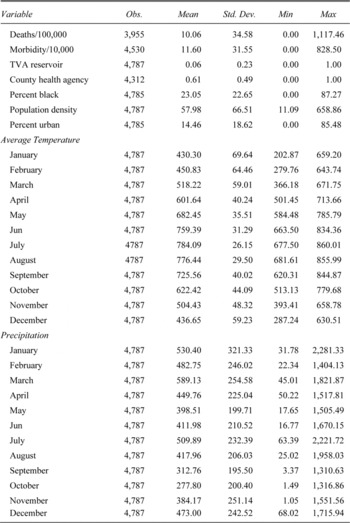
SUMMARY STATISTICS

Notes:
Deaths/100,000 report the average number of malaria deaths per 100,000. Morbidity/10,000 reports the average number of reported malaria cases. Average monthly temperatures are reported in tenths of a degree Fahrenheit. Average monthly precipitation is reported in hundredths of an inch.
Sources:
See the Appendix.
The Tennessee Valley Authority
In May of 1933 President Franklin Delano Roosevelt created the Tennessee Valley Authority. It was chartered as a federal corporation that would assume control of the Tennessee River and its tributaries and promote development in the South. The charter announced that the TVA had a general mandate to improve the economy in the Tennessee Valley. The first director of the TVA, Arthur Morgan, quickly established plans for a series of dams and reservoirs to line the Tennessee River and its major tributaries. The plans expanded an existing U.S. Army Corps of Engineering (USACE) project, Wilson Dam in Muscle Shoals, Alabama and existing Army plans for dams at Cove Creek (Norris Dam) and Wheeler Reservoir. In its first six years, the TVA grew rapidly. By 1939 the TVA had received over $3.68 billion in federal appropriations. By 1951 cumulative appropriations exceeded $14.2 billion. Most of this money was spent on dams and related expenses including land purchases, transmission lines, and electric generation plants.
These projects also raised concerns because they impounded large bodies of water. It was estimated that dams' system of lakes and reservoirs would produce a shoreline 10,000 miles in length covering 600,000 acres of water. This vast shoreline created a large breeding ground for mosquitoes (Derryberry and Gartrell 1952). From the beginning, the TVA tried to mitigate malaria without heavy use of insecticides including introducing natural predators of mosquito larvae, destroying their habitat through drainage and periodic water fluctuations, brush clearing, larvacides, oiling, and eventually DDT (Gartrell and Ludvik 1954, TVA 1945).
Perhaps the TVA's largest effort came through the nearly costless plan to vary the water levels in the reservoirs. During the winter and early spring months, the TVA stored winter rain water at dams located at the top of the watershed. As the mosquito breeding season approached, the TVA released the stored water into downstream reservoirs, raising the water level a few inches. The surge flooded potential breeding grounds for mosquitoes. The following week, the water level in the dam was lowered exposing the mosquito larvae to natural predators. The water that was released was used to flood the shoreline of the next reservoir downstream, thus reducing its infestation. Water levels fluctuated throughout the entire system until the end of the breeding season.
The TVA's efforts to reduce malaria were the largest in the United States in terms of numbers of engineers and experts. As malaria rates began to decline, the TVA was praised for its strong efforts. The Centers for Disease Control (CDC) lists the TVA's accomplishments on its malaria history website.
“An organized and effective malaria control program stemmed from this new authority in the Tennessee River Valley. Malaria affected 30 percent of the population in the region when the TVA was incorporated in 1933… and by 1947 the disease was essentially eliminated. Mosquito breeding sites were reduced by controlling water levels and insecticide applications.”
It is clear that prevalence fell off, but that does imply that the TVA's actions were responsible because other agencies United States Public Health Service (USPHS), Works Progress Administration (WPA), and Malaria Control in War Areas (MCWA). Moreover, the net TVA impact is hard to predict because its action both worsened malaria incidence (dams increased sitting water) and reduced it (via vector control efforts). These factors help to motivate my effort to carefully estimate the net effects of a TVA dams on malaria rates.
CHANGE IN DISEASE RATES
To identify the effect of the TVA on malaria rates in the Southeast United States, I construct a panel data set from county-level disease-specific data. I first outline the baseline specifications to identify the effect of TVA dams on malaria rates assuming that the dams' locations were uncorrelated with prior malaria prevalence. I then show that this assumption of exogeneity holds by regressing the eventual dam locations on pretreatment characteristics. I also discuss historical reasons why malarial prevalence is unlikely to have mattered to the dams' location. I then proceed with fixed-effects regressions which use within-county variation across time, controlling for statewide shocks occurring in specific years to identify the effect of dams on malaria. I do this to control for time-invariant unobserved features in the county and observable time-invariant features, such as geography and topography. State-by-year effects are included to control for state-level changes in malaria reporting or unobserved changes in the structure of the state health system that would affect the malaria data. Given the panel nature of the data employed, I am able to control for a variety of features such as county-specific shocks, year-specific shocks, auto correlation, and correlation across geographic space.
Baseline Empirical Model of Malaria Rate
Let us start with a simple specification:

Where Mit is either the mortality rate per 100,000 people or the morbidity rate per 10,000 people in county i in year t. The vector Ci represents a set of county fixed effects to control for unobservable characteristics such as mountains, altitude, latitude, and longitude. Yi is a vector of year fixed effects that seek to absorb things like region-wide epidemics and widespread shocks affecting the malaria rate.Footnote 3TVAit is an indicator that equals 1 if county i in year t includes at least part of a completed TVA reservoir. Climateit includes monthly average temperatures, monthly precipitation, and an interaction term of the two variables. Xit is a vector of time-varying county-level variables: the presence of a County Health Organization (CHO) to control for changes in access to health care, population density, percent black, and the urbanization rate.
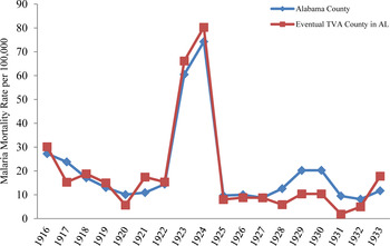
This estimation strategy assumes that malaria was exogenous to and uncorrelated with dams locations—an assumption we will evaluate later. The model also assumes that the trend of disease rates did not differ between counties that received dams and those that did not. Figure 1 evaluates this assumption by showing the average mortality rate in Alabama from 1916–1933 by eventual TVA dam status.Footnote 4 Counties in black represent counties in Alabama that never received a TVA dam and counties in grey are those that eventually obtained a TVA dam. Between 1916 and 1933, prior to the creation of the TVA, there is no difference in the mortality rate between the two types of counties.
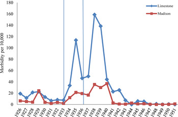
The impact of a dam can be seen in Figure 2, which presents a time series of the malaria morbidity rate for two adjacent counties, Limestone, located on Wheeler Reservoir and Madison, which is not on the reservoir. The first vertical line in Figure 2 denotes the beginning of construction, the second denotes its end. Prior to construction, the two counties had similar morbidity. However, the beginning of construction at Wheeler coincided with a major increase in the malaria morbidity rate in Limestone County. The increase in Limestone County persists through the completion of construction and remains higher than the initial rate for several years to follow. Madison County sees neither the rise nor the fall in malarial incidence. This comparison is just one example of the kind of differences between counties that help identify the effect of the TVA.Footnote 5 While there is a spike following initial construction, I cannot identify systematically the year in which the reservoir began to fill. Therefore the TVA variable is restricted to counties being located on completed reservoirs. Restricting the indicator in this way will bias the coefficient on the impact of the TVA (β1) downward. Other effects will also present potential biases on β1 Dams potentially lead to increases in wealth which in turn could lead to a decrease in the probability of contracting malaria. Dams also change the distribution of the population within the county by removing the population that was living close to the river. Both the income and population removal effects would lead to downward bias of β1. One further complication in the empirical specification is that humans are mobile, possibly leading to spillovers in neighboring regions. This spatial aspect will be examined directly in the robustness checks with the use of spatially weighted regressions.Footnote 6
MALARIA MORTALITY IN ALABAMA, 1916–1935

MALARIA MORBIDITY NEAR WHEELER RESERVOIR

Is the TVA Exogenous to Malaria?
The underlying assumption of the empirical model outlined above is that the dams are randomly located with respect to malaria conditional on a variety of covariates. It is possible that dams are placed in areas that are prone to malaria—either because the TVA targeted these areas for their malarial levels or because the areas geologically most favored for dam building had high malaria incidence. However, the evidence suggests that malaria was not a concern when the TVA located its reservoirs. First, following the great flood of the Mississippi River in 1926/27, the USACE was commissioned to develop a strategy to prevent any recurrence of such disasters. The Corps of Engineers developed a plan to dam the Tennessee River so as to reduce the flood stage waters on the Mississippi River by one foot. This report detailed where dams needed to be built both for flood control and to provide a 9-foot navigation channel from Knoxville, TN to Paducah, KY where the Tennessee runs into the Ohio.Footnote 7 The 1930 USACE report included the engineering drawings for Norris Dam and Wheeler Dam, which TVA engineers used to construct those dams. Other TVA dams also relied on the locations outlined in that report. Although there is plenty of evidence that flood control and navigation played important roles in the placement of dams, there is no such evidence that engineers considered malaria.
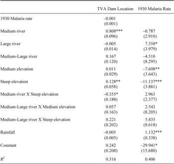
CHARACTERISTICS CORRELATED WITH DAM PLACEMENT AND MALARIA

* p < .10, ** p < .05, *** p < .01.
Notes:
River sizes are classified according to the definitions used in Fishback, Haines, and Kantor (2006). Elevation ranges are calculated by subtracting the maximum and minimum elevation in each county. The elevation categories are then classified as Low Elevation – below the 25th percentile of the sample, Medium Elevation – in the middle 50 percent of the sample, and Steep Elevation – in the top 25 percentile of the sample. Rainfall is the annual rainfall in the county.
Sources:
See the Appendix.
More importantly, the dams were randomly located with respect to pre-TVA malaria rates. Table 2, column 1 shows the results of a linear probability model that estimates the probability of obtaining a TVA reservoir by 1951 on, the presence of various sized rivers, elevation changes within the county, interactions between rivers and land gradients, and the malaria rate in 1930. These results show that dams were placed in areas with medium to large sized rivers and a steep land gradient. These results are consistent with the placement of dams designed to store water and produce electricity. They require steep changes in elevation to generate electricity, or a natural basin formed by the narrowing of the river through mountainous terrain. The results also show that the malaria rate in 1930 is not correlated with the placement of TVA dams.
While the placement of TVA dams is not correlated with malaria, it may be the case that features of the topography where dams are placed are conducive to more malaria. To address this concern, I regress the 1930 malaria rate on geographic characteristics, such as elevation changes, river flow, rainfall, and a full set of interactions between geographic characteristics. The results, presented in Table 2, column 2, show that malaria is correlated with areas that have a relatively flat land gradient, do not have moving water from medium to large sized rivers, and receive large amounts of rainfall. These results suggest that malaria is most prone in areas that are least suitable for large hydroelectric and storage reservoirs. The primary empirical model includes county-level fixed effects to take into account geographic features which do not change over time. However, if there is any correlation remaining, the results will downward bias the negative effect of the TVA on malaria's incidence.
One further concern with the placement of dams is that the USACE placed them in counties with desirable topographic characteristics and where it would be easy to assemble the land the reservoir would flood. If farmers abandoned their land immediately after it was purchased by the TVA, then there would be a large increase of idle agricultural land, which would likely raise malaria's prevalence (Humphreys 2001). Kitchens (2012) evaluates the TVA's use of eminent domain to assemble the properties for the reservoirs. He finds survey evidence that the Authority allowed farmers to stay on the land after it had been purchased. The TVA's typical policy allowed farmers to stay until their piece of property was going to be flooded, limiting the time that land was idle and, consequently, any increase in malaria.
Malaria Prevalence Data
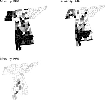
Data has been collected from a variety of state and federal sources for every county in Alabama and Tennessee for the years 1926 through 1951 inclusive. Each year consists of 162 county observations over the 26 years which results in 4,212 county-year observations. Morbidity and mortality for Alabama and Tennessee come from state public health department reports and from the Vital Statistics of the United States.Footnote 8 These state-level reports provide the best insight into the prevalence of disease; however they also have many shortcomings. The earliest state health reports do not report malaria deaths or illnesses by race, and the only data pertaining to the age distribution of deaths is available at the state level in a limited number of years. Nevertheless, the county-level statistics are the best measures available for the time period and were used by policymakers to make decisions about funding and control efforts. For example, in 1945, when state health agencies first allocated DDT to counties, they did so based on average malaria mortality rates from 1938 to 1942 (Alabama State Board of Health 1946, p. 217). While there are some instances of more accurate blood smear surveys in elementary schools, these are few and far between, making county level statistics the most reliable information about malaria during the period. The malaria rate data allows malaria to be measured directly rather than indirectly as in past studies that construct an index of malaria prevalence from climate and geographic variables as in Sok Chul Hong (2007). It should also be noted that the reported rates may actually be a lower-bound estimate of the true prevalence in a county. Reporting of illness only occurred if a person was attended to by a physician. Contemporary malaria experts believed that the true prevalence was between 200 and 400 percent higher than reported rates.Footnote 9 Throughout our period, malaria was in steady decline. It was nearly eradicated by 1950. Figure 3 shows the spatial distribution of malaria mortality in Alabama and Tennessee in from 1930 to 1950. Deaths were heavily concentrated in the warm climates of South Alabama and in the wet regions of the Mississippi River in West Tennessee. The morbidity patterns are very similar.
I use monthly weather variables to control for random weather shocks that would affect malaria rates. To control for this, I have collected the Historic Climatology Networks Monthly Weather data from 1895–2009. This data contains the monthly average, maximum, and minimum temperatures as well as precipitation data collected at each weather station throughout the country. County-level observations were constructed through a triangular interpolation method.Footnote 10
SPATIAL PATTERN OF MALARIA MORTALITY

TVA Annual Reports to Congress provided the locations of reservoirs. By the end of the sample period, 25/162 counties have a TVA reservoir located in their county. Figure 4 show the expansion of treated counties over time as new reservoirs were constructed by the TVA. The majority of counties are in eastern Tennessee and North Alabama, areas which traditionally had low malaria rates.
To proxy for the water level fluctuations from upstream storage reservoirs downstream through the system, I have created a variable that counts the number of reservoirs located upstream from each reservoir county. Upstream dams are necessary if engineers are to artificially alter the water levels so as to reduce the prevalence of malaria. Reservoirs further downstream are likely to gain the most due to increased control over the water level and flow rates through the reservoir.
EXPANSION OF TVA RESERVOIRS
In both Alabama and Tennessee, the State Board of Health had offices in each county. Alabama had started to establish local offices in 1919, and by 1937 it a Board of Health office in every county. These offices aimed to fight a variety of diseases malaria, typhoid, syphilis, and other communicable diseases were at the forefront of importance for the local authorities. But they also were tasked with reducing infant mortality. The opening of a health agency is likely endogenous to malaria, wealth, and other measures of health; however it can be shown that the opening of a CHO and a TVA reservoir are uncorrelated, thus including the presence of a CHO will not bias the estimate for the TVA.
Other New Deal agencies also played a crucial role in the fight against malaria. Kitchens (2012b) shows that work by the WPA in Georgia led to large reductions in malaria during the 1930s. To account for ongoing work by other agencies, I include a set of three variables: New Feet, Old Feet, and Acres Excavated. New Feet refers to the number of linear feet of concrete lined drainage ditch constructed in the county-year. Old feet refers to the number of linear feet of drainage ditches which were cleaned, and Excavated refers number of acres of ponds or swamps filled with dirt or gravel. These measures were reported in Alabama's State Board of Health reported annual progress in counties where federal relief agency labor was used. Margaret Humphreys (2001) suggest that shoddy construction of drainage ditches and poor maintenance of ditches often led to increases in sitting water from sitting debris, whereas filling in swamp land with dirt or filling in ponds reduces the sitting water problem.
Population characteristics are compiled from the Census of Population and from the State Vital Statistics reports. Combining the population and area data provides a measure of the population density per square mile. In the early years of the malaria campaigns, state agencies focused on urban areas, recognizing that a large portion of the population could be affected by malaria fighting efforts. Because malaria is transferred from human to human through mosquito bites, residents of urban counties may be more susceptible to infection. Census data are also be used to determine the percentage of the population that was African American. There are two arguments assessing that malaria's impact might have been racially differentiated. The first is that sickle cell anemia, a genetic mutation concentrated among African Americans, provided resistance to infection and thus that group should have a lower infection rate (Allison 1954; Aidoo 2002). The second argument focuses on the poverty of southern blacks. Blacks may have to live on land closer to swamps and mosquito breeding grounds due to their low income status in the South, putting them at higher risk for contracting malaria (Humphreys 2001). It is unclear if sickle cell or poverty will play the dominating role.
RESULTS
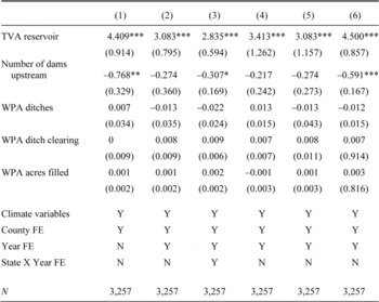
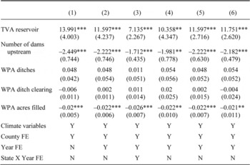
The regression results in Tables 4 and 5 show that the TVA led to medically and statistically significant increases in mortality and morbidity rates. Depending on the specification, the TVA increases mortality rates by 2.8 to 4.4 deaths per 100,000 and increases morbidity rates between 7.1 and 13.9 cases per 10,000. The point estimates represent a 40 to 50 percent increase in malaria mortality relative to the sample mean. This estimate is the net effect of having a TVA reservoir in the county, taking into account the campaigns financed and implemented by TVA as well as all possible channels through which dams affect malaria.
Column 1 of Table 3 presents the OLS results with county fixed effects; the estimated net effect of a TVA reservoir located in a county is a 4.4 increase in the malaria mortality rate. Specification 2 adds year fixed effects, and specification 3 includes state-by-year fixed effects. State-by-year effects may be important to control for changes in the ways reporting occurs, or to capture changes within the structure of the state-level health agency. Even after controlling for a large portion of variation with the inclusion of various fixed effects, the TVA coefficient remains positive and large.
MALARIA MORTALITY REGRESSION RESULTS

* p < .10, ** p < .05, *** p < .01.
Notes:
Specification 4 accounts for AR(1) error structure; Specification 5 clusters error at weather station level; and Specification 6 adjusts for spatial correlation in errors.
As predicted, the number of dams upstream reduces the malaria burden downstream.Footnote 11 This is a direct result of the water level fluctuations which are used to expose mosquito larvae to the elements. In every specification, additional upstream reservoirs are associated with a reduction in the malaria mortality rate, however in some specifications the coefficient is not statistically significant. Other control activities, such as draining and ditching have little effect on mortality rates which is consistent with qualitative evidence. Humphreys (2001) discusses how many of the WPA projects were poorly constructed, leading to stagnate pools of water in drainage ditches.
MALARIA MORBIDITY REGRESSION RESULTS

* p < .10, ** p < .05, *** p < .01.
Notes:
Specification 4 accounts for AR(1) error structure; Specification 5 clusters error at weather station level; and Specification 6 adjusts for spatial correlation in errors.
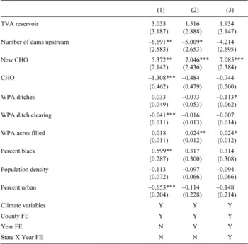
Table 4 presents the full set of morbidity results. Column 1 includes only county fixed effects, column 2 adds year-specific effects, and column 3 state-by-year effects. In each specification, building a TVA reservoir led to statistically significant increase in morbidity. The upstream dams played a crucial role in mitigating malaria morbidity in downstream reservoirs. While having a reservoir in the county increases rates up to 13.9 cases, having a dam located upstream leads to a 1.7–2.4 reduction in the number of cases. For some locations, this could completely offset the malaria increase caused by the TVA reservoirs. Counties located adjacent to head water dams, such as Norris, received no benefits from the water fluctuations, however, as one moves downstream, there is an increasingly positive effect. A dam such as Ft. Loudon, with only one dam upstream only experienced minor benefits from upstream dams, however, a dam like Pickwick, located in Hardin County, TN, eventually had 11 dams located upstream from it. Its malaria rate fell from a high in 1935 (when construction began) of 122 illnesses per 10,000 to zero by 1951.
Parts of other New Deal programs also seem to have been effective at reducing the morbidity rate. The combined efforts by the Civilian Works Administration (CWA), Federal Emergency Relief Administration (FERA), and WPA to excavate dirt to fill and drain swamps led to a statistically significant reduction in the malaria morbidity rate. For every acre of dirt excavated or filled, the resulting reduction in the malaria rate is .02 per 10,000. While excavation appears to have worked, ditching is associated with increases in the malaria rate. The Tennessee Department of Public Health Biennial Reports discusses how some of the ditches constructed were of poor design and led to more debris collecting, exacerbating the problem.
Robustness Checks
The approach I implemented in the main section assumes that malaria rates were not correlated over time or space. Yet one might worry about this assumption because the plasmodium vivax parasite can live in the blood stream for up to three years, so shocks that occur in the past might have affected rates in the future. Tests of the fixed effects residuals indicate that auto correlation only persisted for one period. The auto correlation parameter is estimated using the Prais-Winsten procedure with an AR(1) error process. Results from this regression are presented in Table 3, column 4 for Mortality, and Table 4, column 4 for morbidity. The estimated net effect of a TVA reservoir, accounting for auto correlation, remains positive and statistically significant.Footnote 12 The correlation coefficient across time periods is .295 for mortality and .344 for morbidity; not enough to affect the substantive conclusions of section 3.
A second issue involves spatial spillovers. Some spatial correlation is induced into the model due to the interpolation of climate data. Because the data are interpolated, data in a given county will be correlated across space with other counties sharing the same weather station observation. To account for this, I adopt a method posed by Colin Cameron, Jonah Gelbach, and Doug Miller (2010), which clusters observation along multiple dimensions. The second spatial issue arises from the natural geography. There is a general downward slope from the eastern portion of the sample to the west as water drains towards the Mississippi River. Counties further east, or upstream, may experience improved natural drainage across counties, leading to less sitting water where mosquitoes might breed. As a result, if there is a shock in one area, it could affect other cross sectional observations. To account for this, I reanalyze the data using a spatial error model (Anselin 1988; LeSage and Pace 2009).
Results from the Cameron, Gelbach, and Miller (2010) multidimensional clustering are presented in column 5 of Tables 3 and 4. These regressions are clustered to account for shocks occurring at each of the three weather stations used in the interpolation of the climate variables. The procedure increased standard errors; but not much, and the key variables easily pass a 1 percent significance test leaving the qualitative interpretation of the TVA projects the same.
Spatial spillover may also influence the rate of malaria transmission. Patrick Moran (1950) I tests reveal the potential for spatial correlation in the error structure. To account for spatial spillover, I estimate the model with the inclusion of spatially correlated errors. Column 6 of Tables 3 and 4 presents the results of a spatial error model (SEM). In this model, errors occurring in neighboring cross-sectional units are weighted by proximity to the ith observation.Footnote 13 Taking the spatial dependence into account leaves all the results unchanged. In all specifications, the net effect of the TVA was a large increase in malaria mortality and morbidity.
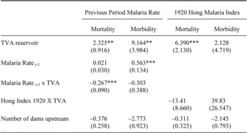
The current empirical specifications, assumes that reservoir construction does not differentially impact counties. However, epidemiological research suggests that the most affected areas would be those with relatively low malaria rates prior to treatment. To determine if there were differential effects of receiving a dam, I modify the empirical specification in two ways. I first run a regression with an interaction between the presence of a reservoir and lagged malaria rates. This may not the most desirable specification as it introduces serial dependence in the error structure. I also run a regression with an interaction term between the presence of a TVA reservoir and the Hong Malaria Index for 1920 (Hong 2007). This index predicts the probability of contracting malaria based on geographic, topographic, and climatic conditions. The results from these regressions are presented in Table 5. Columns 1 and 2 present the results when the previous period malaria rate is interacted with the TVA indicator variable. In this specification, the TVA reservoir point estimate falls, yet remains positive and statistically significant. The results also show that there were differential effects for counties that had high or low levels of malaria prior to the dams' arrivals. If a county had a one point lower death rate, it experienced a .267 increase in the number of deaths per 100,000 individuals when it received a reservoir.Footnote 14 The effect is similar using morbidity as the outcome variable of interest, however it is statistically insignificant. In each additional specification the results remain positive and statistically significant. Columns 3 and 4 of Table 5 display the results when the Hong Index is interacted with the TVA reservoir variable. In this specification, the results also show that areas with a higher likelihood of malaria experienced smaller increases in the malaria mortality and morbidity rate following the completion of a TVA reservoir.
HETEROGENEOUS EFFECTS OF A TVA RESERVOIR

* p < .10, ** p < .05, *** p < .01.
Notes:
Each specification modifies the baseline difference in difference by interacting the TVA treatment variable with the prior period malaria rate or the Hong Index (Hong 2007) from 1920.
Sources:
See the Appendix.
While the results suggest that the introduction of TVA reservoirs increased malaria rates, it may be possible that the entire disease profile is endogenously changing in the counties where the TVA is located. An entire shift in the disease profile might make it appear as though the TVA was the cause of a malaria rate increase when the change in rates was due to an exogenous factor. To examine this hypothesis, I reestimate the model using data pertaining to a different disease.
MEASLES REGRESSION RESULTS

* p < .10, ** p < .05, *** p < .01.
Sources:
See the Appendix.
Measles has several nice properties for the purpose of this exercise. First and foremost, it is not a waterborne disease. Changes in the water environment should not affect the transmission of measles. Furthermore, it is an airborne virus that infects a large portion of the population. Data for measles morbidity rates come from the Alabama State Board of Health Annual Reports and Tennessee Morbidity Report.
In this setting, I substitute the measles morbidity rate in place of the malaria morbidity rate in the baseline empirical model and reestimate the estimating equation. Regression results show that there is no statistically significant link between the TVA reservoirs and measles. The full set of results is presented in Table 6. This suggests that when the TVA entered the region, it only raised malaria rates and not morbidity for other major diseases.
Effects During Dam Construction
The baseline empirical model assumes that the effect of the dam does not occur until construction is finished, however, dams typically take several years to construct and are partially filled at various points in time. Figure 2 hints that construction may also be a treatment, as there is an increase in the malaria rate following the start of construction in 1933 at Wheeler Dam. If there is a construction effect, the baseline estimates presented above would be biased downward due to an inflated pretreatment malaria rate.
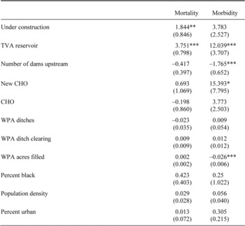
To test the extent to which the construction period biases the estimate, I reestimate the baseline model to include an indicator variable equal to 1 if the project is under construction, but not yet completed. The effect that the construction period has on malaria is not clear a priori. The influx of construction workers to the job site may increase the number of people available to transmit malaria, temporary disruptions in the river and partial flooding may increase sitting water; however income shocks associated with spending on the dam may allow more people to take precautions to avoid malaria. Table 7 presents the estimates and it shows that construction led to increases in the malaria's incidence. During the average dam's construction, the mortality rate increased by 1.8 deaths per 100,000, which is an 18 percent increase over the baseline. After taking into account the effects during construction, I find that the point estimate of a completed TVA reservoir has a larger effect than when the construction period is ignored. Without including the effects of construction, the mortality rate increased by 2.8 deaths per 100,000 people,Footnote 15 with construction effects included, the mortality rate increased by 3.7 deaths per 100,000, which is a 37 percent increase over the period average. The morbidity rate also increased in this specification from 7.13 cases per 10,000 to 12 cases per 10,000.
The Evolution of Malaria over Time
The baseline analysis also assumes that when a reservoir is completed, malaria increases instantly and persists over time. It is possible, however, that the effect of the reservoir on the malaria rate evolves over time, as suggested by Figure 3. I generalize the baseline model to allow for time-varying effects as follows:
CHANGE IN MALARIA INCLUDING CONSTRUCTION EFFECTS

* p < .10, ** p < .05, *** p < .01.
Notes:
Each specification includes state by year fixed effects.
Sources:
See the Appendix.

Where Mit is defined as above, and k is the number of years before or after dam arrival. Because the length of construction varies for each dam, k = −1 is defined as the year before work began, k = 0 is defined as the construction period, and k > 0 is defined as the number of years after construction is completed.Footnote 16
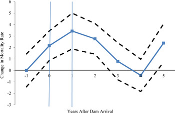
TIME-VARYING EFFECT OF TVA DAMS ON MALARIA MORTALITY

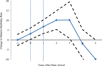
The results of these regressions are best shown in Figures 5 and 6. Figure 5 plots the coefficients for mortality, normalized by setting the preconstruction period equal to zero. Relative to the pretreatment period, mortality rate increases during construction and an even larger spike following completion of the reservoir which persists for three years, after which the malaria rate returns to preconstruction levels. Given that the average dam took three years to construct prior to filling, malaria rates were elevated for six years, leading to a total increase in the mortality rate of 13.4 deaths per 100,000. Similarly, Figure 6 plots the results for morbidity, over the same six-year period, morbidity increased by a total of 38.4 cases per 10,000.
THE COST OF THE TVA
Just how costly was the increased malaria? Combining Value of a Statistical Life (VSL) estimates from the literature with the change in mortality rates allows us to get an estimate of the TVA's cost. I assume that the value of a life was the same in all counties over the whole period. To calculate the malaria cost of the TVA, I use the following formula:
TIME-VARYING EFFECT OF TVA DAMS ON MALARIA MORBIDITY


VSL is an external estimate of the value of a life. The second term adjusts the county population in year t to correspond to the mortality rates. As before, TVA takes on the value one if the county abuts a reservoir, β1 is the estimated change in malaria resulting from a TVA reservoir, is the estimated impact of upstream reservoirs, Δ and upstream is the number of reservoirs upstream from the given county-year. I am thus adding up the number of malaria deaths per TVA county in a given year and then multiplying that total by the VSL.
The mortality estimates that account for state-year fixed effects show that malaria increased by 2.8 deaths per 100,000 individuals per year. Dora Costa and Matthew Kahn (2004) construct estimates for the value of a statistical life during the 1940s. They find that during the period, a life was valued between $1.1 and $1.6 million in 2009 dollars. Using a VSL of $1.1 million, and a rise in mortality of 2.8 deaths per 100,000, the resulting cost, ignoring the effects of upstream dams is $508 million. When upstream effects are included in the calculation, the cost falls to $340 million in lost life.Footnote 17
I use similar methods to calculate the cost attributable to malaria morbidity, these are much smaller. Using the most preferred estimates that include state-by-year fixed effects; morbidity increased by 7.1 cases per 10,000 individuals. Using external estimates reported by the Atlanta Journal Constitution at the time, a case of malaria cost $45 in lost wages, or approximately two weeks of labor.Footnote 18 After adjusting the estimates to 2009 dollars and using the formula above, I find that the TVA morbidity cost was $7.4 million in lost income over the sample period when upstream effects are ignored. When upstream effects are included, the cost falls to $1.7 million.
How large is the loss of life from malaria relative to the size of the TVA? The typical TVA story is one in which a regionally targeted development agency spurs growth through low electricity prices leading to spillovers in other industries. By 1951 about $14.2 billion had been spent in the Tennessee Valley by the TVA. Recent work by Kitchens (2012a) shows that the TVA did not lead to faster growth relative to areas not electrified by the TVA and did not lead to lower electric rates than comparable private firms. Patrick Kline and Enrico Moretti (2012) show that in the short run, the TVA did little to stimulate local economies and more likely led to shifts in employment from agriculture to manufacturing, Kline and Moretti (2012) also note that any gains from the TVA are likely short-run phenomena and will diminish in the long run.
This suggests that the federal spending on the TVA may be the reference point for the benefits that are derived from the TVA. Price Fishback and Valentina Kachanovskaya (2012) note that during the New Deal, the fiscal spending multiplier was 1.1, so the roughly $14.2 billion spent on the TVA would yield $15.6 billion in total benefits, or $1.4 billion in additional benefits beyond the direct spending. Using the most conservative cost calculations of $340 million, the malaria cost would represent 2.1 percent of all TVA appropriations and multiplied benefits. If the TVA generated $1.4 billion in benefits through fiscal stimulus, the malaria cost reduces the benefit by 24 percent. If the correct VSL is on the higher end of the literature, the malaria cost would represent 23.7 percent of total TVA benefits, and would more than offset the fiscal multiplier effect. In this scenario, the region would be better off receiving direct cash transfers rather than constructing the infrastructure.
CONCLUSIONS
Given the recent focus of providing infrastructure in developing nations, it is important to understand the unintended consequences of investment. In particular, when large dams are built to provide electricity they change the local environment which may affect disease prevalence. This article examines these issues through for the TVA, which was one of the largest regionally focused development projects in U.S. history. Using malaria rates constructed from state level health publications. I first demonstrate that dam location and timing decisions were uncorrelated with malaria's prevalence and I then find that reservoirs built by the TVA drove the malaria morbidity and mortality rates up. The increase in malaria rates was large and implies a significant hidden cost, 24 percent of the fiscal stimulus, due to illness and the loss of life.
The TVA provides insight into a growing problem around the world today. As more developing nations build large water management programs, increased sitting water is liable to raise rates of infectious disease. The TVA, which was long held in esteem for tackling the malaria problem in the Southeast, had to take action because its reservoir expanded the sitting water in the region. These increases in sitting water provided new breeding ground for mosquitoes, which ultimately led to a surge in malaria despite the largest anti-malaria efforts to date on the behalf of the TVA. Almost certainly the problem would have been more severe had the TVA not made an attempt to control the disease by spraying, ditching, and fluctuation of the water level in its reservoirs.
Specific attention should be given to the method of raising and lowering the water levels from reservoir to reservoir. There is support that this method reduced the malaria problem. This method can be used at low cost and is easily implemented. A note of caution, the TVA storage reservoirs upstream were typically located in mountainous areas, which are less susceptible to malaria due to their higher elevations and cooler climates. Attempting upstream water storage for mosquito prevention may not work as well in areas with warmer and wetter climates or lower elevations.
Data Appendix
Malaria Rates: Malaria mortality and morbidity rate data are reported in several state and federal publications. In Alabama, data was collected from Alabama State Board of Health Annual and Biennial Reports, 1914–1951. To supplement these reports, I also collected malaria data from the Alabama Vital Statistics reports, 1929–1946. This report changed names several times throughout the sample period. To supplement these rates, I also consulted the Vital Statistics of the United States Part II. Natality and Mortality Data for the United States, 1943–1948. In Tennessee, I collected malaria mortality and morbidity data from Tennessee Department of Public Health Annual Bulletin of Vital Statistics, 1927–1951, the Tennessee Department of Public Health Annual Report, 1926–1941 and Tennessee Department of Public Health: Tennessee Morbidity Statistics, 1931–1951. In certain years, the U.S. Vital Statistics were collected to supplement the Tennessee Vital Statistics.
Measles Data: Measles morbidity rate data are reported in several state and federal publications. In Alabama, data was collected from Alabama State Board of Health Annual and Biennial Reports, 1914–1951. In Tennessee, I collected measles morbidity data from Tennessee Department of Public Health. Annual Report, 1926–1941 and the Tennessee Department of Public Health: Tennessee Morbidity Statistics, 1931–1951.
Climate Data: Climate data were collected from the U.S Historic Climatology Network. Monthly Data, 1895–2009, http://cdiac.ornl.gov/ftp/ushcn_v2_monthly/. This data was then interpolated using a triangular weighting method in order to construct monthly county-level observations.
Location of TVA Dams: This data was collected from the TVA Annual Reports, 1934–1951.
Geographic Characteristics: Geographic data was collected from Fishback, Haines, and Kantor (2007).
Economic and Demographic Variables: Census variables reported by Haines (2004) were used to construct demographic measures.
Presence of County Health Organization: Alabama State Board of Health Annual and Biennial Report, 1914–1951. Tennessee Department of Public Health Annual Report, 1926–1941.
Works Progress Administration Projects: This data was reported in the Alabama State Board of Health Annual Report, 1926–1951.