1 Introduction
Katabatic slope flows are gravity-driven winds that are common over continental-scale ice sheets or over snow-covered mountainous terrain where cold air flows downhill. Katabatic winds play a vital role in reliable weather predictions pertaining to air quality, aviation and agriculture. A landmark study in understanding of katabatic winds is that of Prandtl (Reference Prandtl1942), in which an analytical solution was developed for a viscous stably stratified quiescent fluid over an infinitely long and uniformly cooled planar surface with a constant slope to it. Despite its simplicity, Prandtl’s solution exhibits the vertical structure of katabatic winds observed in nature. The buoyancy and velocity profile predicted by Prandtl’s laminar flow solution is an exponentially dampened sinusoidal wave with growing height (Fedorovich & Shapiro Reference Fedorovich and Shapiro2009). The solution produces a low-level strong jet along the slope descent, which is capped by a weak reverse flow, as depicted in figure 1.
Despite its usefulness in explaining katabatic slope flows, the linear stability of the Prandtl model and the parameter space in which the underlying assumptions hold have not been investigated in the open literature. Fedorovich & Shapiro (Reference Fedorovich and Shapiro2009) introduced an integral slope flow Reynolds number,
 $Re_{I}$
, that is a function of the slope angle, Brunt–Väisälä frequency, surface buoyancy flux and the kinematic viscosity. They performed direct numerical simulation (DNS) of fully developed turbulence with
 $Re_{I}$
ranging from 3000 to 10 000. Umphrey, DeLeon & Senocak (Reference Umphrey, DeLeon and Senocak2017) adopted the same definition of the Reynolds numbers and conducted laminar katabatic flow computations for
 $Re_{I}=20$
to validate and verify a Navier–Stokes solver. In Shapiro & Fedorovich (Reference Shapiro and Fedorovich2014), it was hypothesised that katabatic slope flows are governed by two independent dimensionless parameters, namely Reynolds and Prandtl numbers. The slope angle appeared as a stretching factor in their Reynolds number definition because Shapiro & Fedorovich worked with boundary-layer approximated equations. As we show in the next section, linear stability of the Prandtl model strongly depends on three non-dimensional parameters, which are the slope angle, the Prandtl number, and a new dimensionless parameter that we introduce in § 3.
Sketch of the slope flow and the rotated coordinate system.

Recently, a number of numerical and experimental studies have been devoted to study instabilities in stably stratified fluid cases. Facchini et al. (Reference Facchini, Favier, Le Gal, Wang and Le Bars2018) investigated linear instability of Couette flow with stable stratification via both experiments and DNS, whereas Chen, Bai & Le Dizès (Reference Chen, Bai and Le Dizès2016) studied stably stratified horizontal boundary layers on a vertical wall; in both cases, the direction of stratification was orthogonal to both the shear and base-flow directions. The case where the direction of stratification was orthogonal to the base-flow direction but makes an angle with the plane of shear was analysed by Candelier, Le Dizès & Le Dizès (Reference Candelier, Le Dizès and Millet2011), who identified inviscid instabilities generated by a Bickley jet ejected onto a sloping surface. The Prandtl model for slope flows is uniquely different from these cases as the direction of stratification is oblique to both the base-flow direction and the direction of shear due to the inclination of the surface. In the aforementioned studies, linear stability analysis (LSA) has been used to identify the stability limits. Here, we follow the same general strategy to identify the instabilities and conduct DNS to support the findings of the LSA and visualise the nature of flow instabilities.
2 Governing equations
The idealised slope flow configuration is shown in figure 1, where
 $\unicode[STIX]{x1D6FC}$
is the constant slope angle and gravity acts in the vertical direction.
 $B_{s}$
is the constant heat flux imposed on the surface. For ease of analysis, the problem is studied in a rotated Cartesian coordinate system whose
 $x$
axis is aligned with the planar inclined surface. Let
 $u$
be the along-slope (longitudinal),
 $v$
be the cross-slope (transverse), and
 $w$
be the slope-normal velocity components, such that
 $u_{i}=[u,v,w]$
is the velocity vector. The gravity vector in the rotated coordinate system is then given by
 $g_{i}=[g_{1},g_{2},g_{3}]=[\sin \unicode[STIX]{x1D6FC},0,\cos \unicode[STIX]{x1D6FC}]$
. The buoyancy and the Brunt–Väisälä frequency are denoted by
 $b,N$
, respectively, where
 $N^{2}$
is used as a measure of stratification. Following the presentation in Fedorovich & Shapiro (Reference Fedorovich and Shapiro2009), the momentum and the buoyancy balance equations with a Boussinesq approximation are written as follows:
 $$\begin{eqnarray}\displaystyle & \displaystyle \frac{\unicode[STIX]{x2202}u_{i}}{\unicode[STIX]{x2202}t}+\frac{\unicode[STIX]{x2202}u_{i}u_{j}}{\unicode[STIX]{x2202}x_{j}}=~-\frac{1}{\unicode[STIX]{x1D70C}}\frac{\unicode[STIX]{x2202}p}{\unicode[STIX]{x2202}x_{i}}+\frac{\unicode[STIX]{x2202}}{\unicode[STIX]{x2202}x_{j}}\left(\unicode[STIX]{x1D708}\frac{\unicode[STIX]{x2202}u_{i}}{\unicode[STIX]{x2202}x_{j}}\right)+bg_{i}, & \displaystyle\end{eqnarray}$$
 $$\begin{eqnarray}\displaystyle & \displaystyle \frac{\unicode[STIX]{x2202}b}{\unicode[STIX]{x2202}t}+\frac{\unicode[STIX]{x2202}bu_{j}}{\unicode[STIX]{x2202}x_{j}}=\frac{\unicode[STIX]{x2202}}{\unicode[STIX]{x2202}x_{j}}\left(\unicode[STIX]{x1D6FD}\frac{\unicode[STIX]{x2202}b}{\unicode[STIX]{x2202}x_{j}}\right)-N^{2}g_{j}u_{j}, & \displaystyle\end{eqnarray}$$
where
 $\unicode[STIX]{x1D708},\unicode[STIX]{x1D6FD}$
are the kinematic viscosity and thermal diffusivity of the fluid, respectively. The conservation of mass principle is imposed by a divergence-free velocity field
 $$\begin{eqnarray}\displaystyle \frac{\unicode[STIX]{x2202}u_{i}}{\unicode[STIX]{x2202}x_{i}}=0. & & \displaystyle\end{eqnarray}$$
In the following, the position and velocity vector components
 $x_{i},u_{i}$
are denoted as
 $[x,y,z]^{\text{T}}$
and
 $[u,v,w]^{\text{T}}$
, respectively. Buoyancy is related to the potential temperature as
 $b=g\unicode[STIX]{x1D703}/\unicode[STIX]{x1D6E9}_{r}$
, where
 $\unicode[STIX]{x1D6E9}_{r}$
is a reference potential temperature value. At the surface, a negative buoyancy flux
 $B_{s}$
is imposed to create katabatic flow conditions.
In the Prandtl model, equation (2.1) reduces to a balance between buoyancy and diffusion of along-slope momentum; and (2.2) reduces to a balance between along-slope momentum and diffusion of buoyancy. For the case with a constant buoyancy flux at the surface, Shapiro & Fedorovich (Reference Shapiro and Fedorovich2004) provides the following one-dimensional exact solution:
 $$\begin{eqnarray}\displaystyle & \displaystyle u_{n}=\sqrt{2}\sin (z_{n}/\sqrt{2})\exp (-z_{n}/\sqrt{2}), & \displaystyle\end{eqnarray}$$
 $$\begin{eqnarray}\displaystyle & \displaystyle b_{n}=\sqrt{2}\cos (z_{n}/\sqrt{2})\exp (-z_{n}/\sqrt{2}), & \displaystyle\end{eqnarray}$$
where
 $z_{n}=z/l_{0}$
,
 $u_{n}=u/u_{0}$
,
 $b_{n}=b/b_{0}$
are non-dimensional height, velocity, and buoyancy, respectively, and the corresponding scales governing the flow problem are given as (Fedorovich & Shapiro Reference Fedorovich and Shapiro2009)
 $$\begin{eqnarray}\displaystyle & \displaystyle l_{0}=(\unicode[STIX]{x1D708}\unicode[STIX]{x1D6FD})^{1/4}N^{-1/2}\sin ^{-1/2}\unicode[STIX]{x1D6FC}, & \displaystyle\end{eqnarray}$$
 $$\begin{eqnarray}\displaystyle & \displaystyle u_{0}=(\unicode[STIX]{x1D708}\unicode[STIX]{x1D6FD})^{-1/4}N^{-3/2}B_{s}\sin ^{-1/2}\unicode[STIX]{x1D6FC}, & \displaystyle\end{eqnarray}$$
 $$\begin{eqnarray}\displaystyle & \displaystyle b_{0}=\unicode[STIX]{x1D708}^{1/4}\unicode[STIX]{x1D6FD}^{-3/4}N^{-1/2}B_{s}\sin ^{-1/2}\unicode[STIX]{x1D6FC}, & \displaystyle\end{eqnarray}$$
where
 $Pr\equiv \unicode[STIX]{x1D708}/\unicode[STIX]{x1D6FD}$
is the Prandtl number. A time scale
 $t_{0}=l_{0}/u_{0}$
can also be defined from the above scales. Note that the above flow scales have different forms for the case with a constant buoyancy condition at the surface.
3 Linear stability analysis
Linearising (2.1)–(2.3) around Prandtl’s laminar solution given by (2.4) and (2.5), and assuming that disturbances to the base flow given by Prandtl’s solution are waves of the form
 $\boldsymbol{q}(x,y,z,t)=\hat{\boldsymbol{q}}(z)\exp \{\text{i}(k_{x}x+k_{y}y)+\unicode[STIX]{x1D714}t\}$
, the resulting equations have the form
 $$\begin{eqnarray}\displaystyle & \displaystyle \text{i}k_{x}\hat{u} +\text{i}k_{y}\hat{v}+\frac{\unicode[STIX]{x2202}{\hat{w}}}{\unicode[STIX]{x2202}z}=0, & \displaystyle\end{eqnarray}$$
 $$\begin{eqnarray}\displaystyle & \displaystyle \unicode[STIX]{x1D714}\hat{u} +\text{i}u_{n}k_{x}\hat{u} +u_{n}^{\prime }{\hat{w}}=-\text{i}k_{x}\hat{p}+\frac{Pr}{\unicode[STIX]{x1D6F1}_{s}}\sin \unicode[STIX]{x1D6FC}\left(-(k_{x}^{2}+k_{y}^{2})\hat{u} +\frac{\unicode[STIX]{x2202}^{2}\hat{u} }{\unicode[STIX]{x2202}z^{2}}+\hat{b}\right), & \displaystyle\end{eqnarray}$$
 $$\begin{eqnarray}\displaystyle & \displaystyle \unicode[STIX]{x1D714}\hat{v}+\text{i}u_{n}k_{x}\hat{v}=-\text{i}k_{y}\hat{p}+\frac{Pr}{\unicode[STIX]{x1D6F1}_{s}}\sin \unicode[STIX]{x1D6FC}\left(-(k_{x}^{2}+k_{y}^{2})\hat{v}+\frac{\unicode[STIX]{x2202}^{2}\hat{v}}{\unicode[STIX]{x2202}z^{2}}\right), & \displaystyle\end{eqnarray}$$
 $$\begin{eqnarray}\displaystyle & \displaystyle \unicode[STIX]{x1D714}{\hat{w}}+\text{i}u_{n}k_{x}{\hat{w}}=-\frac{\unicode[STIX]{x2202}\hat{p}}{\unicode[STIX]{x2202}z}+\frac{Pr}{\unicode[STIX]{x1D6F1}_{s}}\sin \unicode[STIX]{x1D6FC}\left(-(k_{x}^{2}+k_{y}^{2}){\hat{w}}+\frac{\unicode[STIX]{x2202}^{2}{\hat{w}}}{\unicode[STIX]{x2202}z^{2}}+\hat{b}\cot \unicode[STIX]{x1D6FC}\right), & \displaystyle\end{eqnarray}$$
 $$\begin{eqnarray}\displaystyle & \displaystyle \unicode[STIX]{x1D714}\hat{b}+\text{i}u_{n}k_{x}\hat{b}+b_{n}^{\prime }{\hat{w}}=\frac{\sin \unicode[STIX]{x1D6FC}}{\unicode[STIX]{x1D6F1}_{s}}\left(-(k_{x}^{2}+k_{y}^{2})\hat{b}+\frac{\unicode[STIX]{x2202}^{2}\hat{b}}{\unicode[STIX]{x2202}z^{2}}-(\hat{u} +{\hat{w}}\cot \unicode[STIX]{x1D6FC})\right), & \displaystyle\end{eqnarray}$$
where
 $\hat{u} ,\hat{v},{\hat{w}},\hat{p},\hat{b}$
are slope-normal-dependent flow disturbances normalised by the flow scales given in (2.6)–(2.8).
 $k_{x},k_{y}$
are real wavenumbers in the
 $x$
(along-slope) and
 $y$
(transverse) directions, respectively, whereas
 $\unicode[STIX]{x1D714}$
is a complex frequency. The normalised Prandtl base-flow solution and its derivative in the slope-normal direction in normalised coordinates are denoted by
 $u_{n},b_{n}$
and
 $u_{n}^{\prime },b_{n}^{\prime }$
, respectively. It can be seen from (2.4)–(2.5) that Prandtl’s laminar velocity profile is a dampened sinusoidal oscillation, thus containing infinitely many inflection points, which opens the possibility of inviscid instabilities. From (3.1)–(3.5), it is clear that there are three dimensionless parameters characterising the idealised katabatic slope flow, which can also be confirmed independently by applying the Buckingham
 $\unicode[STIX]{x03C0}$
theorem. These dimensionless parameters are: Prandtl number
 $Pr$
, slope angle
 $\unicode[STIX]{x1D6FC}$
, and a newly introduced stratification perturbation parameter
 $\unicode[STIX]{x1D6F1}_{s}$
, which is a measure of the ratio between the imposed surface buoyancy gradient and the background stratification. This unique parameter is determined from the externally imposed flow parameters as follows:
 $$\begin{eqnarray}\unicode[STIX]{x1D6F1}_{s}\equiv \frac{|B_{s}|\unicode[STIX]{x1D6FD}^{-1}}{N^{2}}=\frac{\left|{\displaystyle \frac{\unicode[STIX]{x2202}b}{\unicode[STIX]{x2202}z}}(0)\right|}{N^{2}}.\end{eqnarray}$$
Since the buoyancy flux at the surface,
 $B_{s}$
, is negative for katabatic slope flows and positive for anabatic slope flows, the magnitude of
 $B_{s}$
is used in the definition of
 $\unicode[STIX]{x1D6F1}_{s}$
. The slope flow is expected to become dynamically more unstable at higher
 $\unicode[STIX]{x1D6F1}_{s}$
. Note that
 $\unicode[STIX]{x1D6F1}_{s}$
can also be related to the so-called internal Froude number as
 $\unicode[STIX]{x1D6F1}_{s}=Fr\sqrt{Pr}$
, and to the bulk Richardson number as
 $\unicode[STIX]{x1D6F1}_{s}=\sqrt{Pr/Ri}$
. In relating
 $\unicode[STIX]{x1D6F1}_{s}$
to
 $Ri$
and
 $Fr$
, we have used the internal length and velocity scales defined in (2.6) and (2.7), respectively. However, use of
 $Fr$
or
 $Ri$
are not preferred for the current flow problem because there are no externally imposed velocity or length scales.
It is important to mention that
 $\unicode[STIX]{x1D6F1}_{s}$
shares common terms with the flow forcing parameter,
 $Fp_{B}\equiv B_{s}\unicode[STIX]{x1D708}^{-1}/N^{2}$
, that was introduced in Fedorovich & Shapiro (Reference Fedorovich and Shapiro2009). The apparent difference between these two dimensionless parameters is that thermal diffusivity,
 $\unicode[STIX]{x1D6FD}$
, is used in
 $\unicode[STIX]{x1D6F1}_{s}$
, whereas kinematic viscosity,
 $\unicode[STIX]{x1D708}$
, is used in
 $Fp_{B}$
. The physical interpretations of these dimensionless parameters are different. Fedorovich & Shapiro interpreted
 $Fp_{B}$
as the ratio between the energy production at the surface and the work against buoyancy as well as viscous forces. In our proposition, we interpret
 $\unicode[STIX]{x1D6F1}_{s}$
as the degree of disturbance to the background stable stratification by heat conduction at the surface, which is also evident by the appearance of
 $\unicode[STIX]{x1D6F1}_{s}$
in (3.5). These two dimensionless parameters are related to each other through the Prandtl number as
 $\unicode[STIX]{x1D6F1}_{s}=PrFp_{B}$
. As we show later in § 3.3, stability characteristics of slope flows depend strongly on the Prandtl number. Therefore, in our view,
 $Fp_{B}$
and
 $\unicode[STIX]{x1D6F1}_{s}$
are distinct dimensionless parameters with unique interpretations.
The linearised equations can be written as a generalised eigenvalue problem as follows:
 $$\begin{eqnarray}\displaystyle A(k_{x},k_{y})\hat{\boldsymbol{q}}(z)=\unicode[STIX]{x1D714}\boldsymbol{M}\hat{\boldsymbol{q}}(z), & & \displaystyle\end{eqnarray}$$
where
 $\hat{\boldsymbol{q}}(z)=[\hat{u} (z),\hat{v}(z),{\hat{w}}(z),\hat{p}(z),\hat{b}(z)]^{\text{T}}$
is the vector of flow disturbances varying in the slope-normal direction.
 $\boldsymbol{M}$
is a singular matrix arising from the primitive variable formulation; it is created from the identity matrix by setting all diagonal entries belonging to the continuity equation to zero. The appropriate boundary conditions for this problem are no-slip for disturbance velocities at
 $z=0$
, free slip at
 $z\rightarrow \infty$
, and for buoyancy disturbance
 $\unicode[STIX]{x2202}\hat{b}/\unicode[STIX]{x2202}z|_{0}=0,\hat{b}|_{z\rightarrow \infty }=0$
are imposed. The pressure disturbance
 $\hat{p}$
is also set to zero at both
 $z=0$
and
 $z\rightarrow \infty$
. The generalised eigenvalue problem (3.7) is solved via a collocated spectral method using Chebychev polynomials and an algebraic map to cover the semi-infinite domain
 $[0,\infty )$
. Two hundred collocation points are used for discretisation, and the resulting generalised eigenvalue problem is solved with the help of the eigs function in MATLAB. Linear stability of the problem is associated with the real part of the eigenvalues
 $\unicode[STIX]{x1D714}$
, where
 $\text{Re}\{\unicode[STIX]{x1D714}\}>0$
represents a positive exponential growth for the corresponding eigenmode, thus an unstable mode. The imaginary part of
 $\unicode[STIX]{x1D714}$
is the temporal oscillation frequency for the corresponding eigenmode, and
 $\text{Im}\{\unicode[STIX]{x1D714}\}=0$
represents a stationary mode.
3.1 Linear growth rates
To explore the linear instability mechanism dependent on the longitudinal and transverse wavenumbers, the maximal real value of the spectrum for a range of normalised wavenumber vectors
 $(k_{x},k_{y})$
is calculated at various fixed values of
 $\unicode[STIX]{x1D6FC}$
and
 $\unicode[STIX]{x1D6F1}_{s}$
. Since our interest is in katabatic winds we assume
 $Pr=0.71$
, which is a suitable value for air at approximately
 $2\,^{\circ }\text{C}$
. For a slope angle of
 $\unicode[STIX]{x1D6FC}=3^{\circ }$
and
 $\unicode[STIX]{x1D6F1}_{s}=1.66$
, the maximal possible growth rates for wavenumber vectors
 $[k_{x},k_{y}]$
within the interval
 $[0,0.065]\times [0,0.5]$
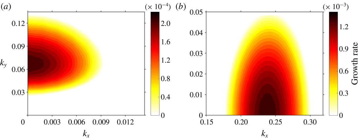
are shown in figure 2(a). Only the positive growth rates, i.e. unstable modes, are highlighted. It can be seen that the growth rates tend to grow with decreasing
 $k_{x}$
component such that the maximal instabilities occur at
 $k_{x}=0$
, i.e. the most unstable modes are purely along the direction transverse to the base-flow direction; the transverse wavenumber at which maximal possible growth rate is attained is valued at approximately
 $k_{y}\approx 0.33$
, as evident from an inspection of the
 $k_{y}$
-axis of figure 2(a). The imaginary part of the eigenvalues corresponding to the maximal positive growth rates are all zero, which indicates that the transverse instabilities studied here are all stationary vortex rolls. This behaviour is in stark contrast to other parallel flows such as the plane Poiseuille flow, for which Squire’s theorem stipulates that the most unstable mode propagates parallel to the direction of the base flow (Schmid & Henningson Reference Schmid and Henningson2001). Thus, it could be inferred that the negative buoyancy force acting simultaneously orthogonal as well as parallel to the base-flow direction is responsible for the transverse mode of instability, which is analogous to the role centrifugal force plays in other types of similar instabilities, such as Görtler vortices or vortices appearing in Taylor–Couette flow (Taylor Reference Taylor1923; Schmid & Henningson Reference Schmid and Henningson2001). For instance, in an earlier work by Görtler (Reference Görtler1959), the normal buoyancy force as well as surface curvature have both been identified as key ingredients for the creation of longitudinal vortices on a curved, cooled surface. From the results of our work, it can be seen that even in the presence of stable stratification with strength
 $N^{2}$
, if the buoyancy force due to surface cooling is sufficiently strong, as measured by the perturbation parameter
 $\unicode[STIX]{x1D6F1}_{s}$
, then the aforementioned instability mechanism inherent in the unstratified cases will be able to overcome the stable background stratification.
Growth rate contours depending on wavenumber vectors
 $k_{x},k_{y}$
for
 $Pr=0.71$
. (a)
 $\unicode[STIX]{x1D6FC}=3^{\circ }$
,
 $\unicode[STIX]{x1D6F1}_{s}=1.6$
; (b)
 $\unicode[STIX]{x1D6FC}=66^{\circ }$
,
 $\unicode[STIX]{x1D6F1}_{s}=18.5$
.
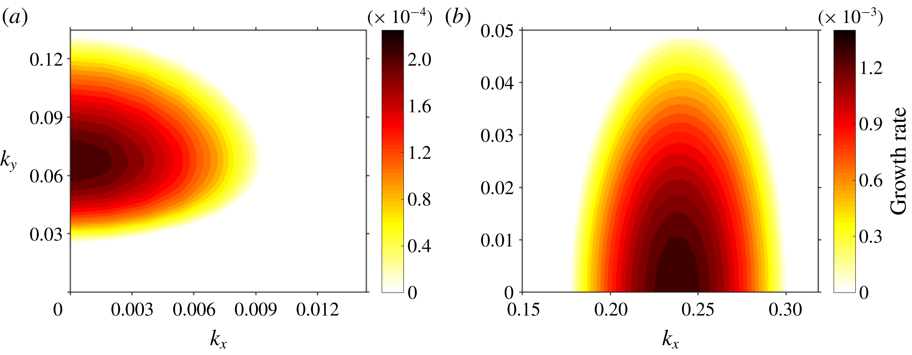
At the steep slope angle of
 $\unicode[STIX]{x1D6FC}=66^{\circ }$
and with a higher stratification perturbation number of
 $\unicode[STIX]{x1D6F1}_{s}=18.5$
, the maximal possible growth rates for wavenumber vectors
 $[k_{x},k_{y}]$
within the interval
 $[0.15,0.33]\times [0,0.05]$
are displayed in figure 2(b). In contrast to the situation at
 $\unicode[STIX]{x1D6FC}=3^{\circ }$
, figure 2(b) shows that the growth rates tend to increase with decreasing
 $k_{y}$
component such that the maximal instabilities occur at
 $k_{y}=0$
; the longitudinal wavenumber at which maximal possible growth rate is attained is valued at approximately
 $k_{x}\approx 0.24$
, as evident from figure 2(b). The most unstable mode are hence purely along the slope direction, parallel to the base-flow direction. This behaviour agrees with instability in other types of parallel flow such as plane Poiseuille flow or Rayleigh–Benard convection. This major deviation from the behaviour of slope flows at the moderate slope angle of
 $\unicode[STIX]{x1D6FC}=3^{\circ }$
could be attributed to the stronger longitudinal gravity component which dominates the stable stratification orthogonal to it at steeper slope angles. Another difference from the moderate slope case (i.e.
 $\unicode[STIX]{x1D6FC}=3^{\circ }$
) is that the imaginary part, i.e. normalised oscillation frequency of the most unstable mode, is approximately 0.115. Thus, in contrast to the transverse instability at moderate slope angles, the longitudinal instability on steep slopes is non-stationary. In both the moderate as well as the steep slope configurations, however, the most unstable instability mode propagates either parallel (
 $k_{y}=0$
) or orthogonal (
 $k_{x}=0$
) to the along-slope direction, but never in an oblique direction(
 $k_{x},k_{y}\neq 0$
), which is a different behaviour than oblique instabilities observed in the spanwise-stratified Couette flow studied by Facchini et al. (Reference Facchini, Favier, Le Gal, Wang and Le Bars2018).
Growth rate contours at
 $\unicode[STIX]{x1D6FC}=3^{\circ }$
for (a) transverse and (b) longitudinal modes and at
 $\unicode[STIX]{x1D6FC}=66^{\circ }$
for (c) longitudinal and (d) transverse modes. The most unstable eigenvalue (
 $\unicode[STIX]{x1D714}\approx 6.6\times 10^{-4}$
) for the transverse mode with
 $k_{y}=0.12$
is highlighted with the marker T in (a). The most unstable eigenvalue (
 $\unicode[STIX]{x1D714}\approx 0.0013+0.115i$
) for the longitudinal mode with
 $k_{x}=0.25$
is highlighted with the marker L in (d). DNS are performed for these two marked cases in § 4.

3.2 Neutral curves and critical stability
The results from the previous subsection support the assertion that the most unstable modes at each slope angle
 $\unicode[STIX]{x1D6FC}$
and stratification perturbation
 $\unicode[STIX]{x1D6F1}_{s}$
are propagating along either the base-flow direction or the transverse direction, i.e. only one component of the wavenumber vector
 $[k_{x},k_{y}]$
is non-zero in order to attain maximal growth rates. Based on this discovery, the critical
 $\unicode[STIX]{x1D6F1}_{s}$
for the onset of instability at a specific slope angle
 $\unicode[STIX]{x1D6FC}$
and
 $Pr$
number can be found by plotting the growth rate contours over a range of
 $\unicode[STIX]{x1D6F1}_{s}$
separately for
 $k_{x}$
and
 $k_{y}$
, assuming that the other wavenumber is zero, respectively. In the following, a constant
 $Pr=0.71$
is assumed. For
 $\unicode[STIX]{x1D6FC}=3^{\circ }$
, the results are shown in figure 3(a,b). It can be seen that the minimal
 $\unicode[STIX]{x1D6F1}_{s}$
for the transverse mode is approximately 5, whereas the longitudinal mode requires a minimal
 $\unicode[STIX]{x1D6F1}_{s}=15.3$
to become unstable. Thus, the most dominant instability in this case is the transverse mode, in agreement with growth rate analysis of the previous subsection (see figure 2
a). In figure 3(c,d), the results for a steep angle of
 $\unicode[STIX]{x1D6FC}=66^{\circ }$
are displayed. This time, it can be observed that the minimal
 $\unicode[STIX]{x1D6F1}_{s}$
for the longitudinal mode is approximately
 $17$
, whereas the transverse mode requires a minimal
 $\unicode[STIX]{x1D6F1}_{s}\approx 19.5$
to become unstable. This means that in contrast to the case of shallower slope angle, the instability to be triggered first at
 $\unicode[STIX]{x1D6FC}=66^{\circ }$
extends along the slope direction parallel to the base flow, which is also supported by the previous growth rate analysis and figure 2(b). In all cases, it can be observed from figure 3 that the unstable growth rates increase with increasing
 $\unicode[STIX]{x1D6F1}_{s}$
, hence pointing to general instability at
 $\unicode[STIX]{x1D6F1}_{s}\rightarrow \infty$
or
 $\unicode[STIX]{x1D708}\rightarrow 0$
. This implies that the instability mechanism must be caused by an inviscid mechanism due to the oscillatory profile of Prandtl’s laminar solution.
3.3 Dependence on the slope angle and the Prandtl number
The previous subsections have demonstrated a drastic change in the nature of the flow instability with increasing slope angle, characterised by a switch from the transverse to the longitudinal direction at sufficiently steep angle due to the increasing longitudinal gravity component driving the flow. To further explore the influence of slope angle,
 $\unicode[STIX]{x1D6FC}$
, on the instability, the critical stability threshold of
 $\unicode[STIX]{x1D6F1}_{s}$
for both longitudinal and transverse instabilities as functions of
 $\unicode[STIX]{x1D6FC}$
over the interval
 $[5^{\circ },80^{\circ }]$
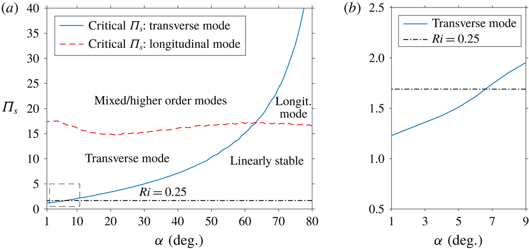
are determined and displayed in figure 4(a). It can be clearly observed that while the critical stratification perturbation parameter,
 $\unicode[STIX]{x1D6F1}_{s}$
, for the transverse instability is lower at shallow angles, it increases for increasing
 $\unicode[STIX]{x1D6FC}$
, and the critical value for the longitudinal instability stays almost constant over the same range of slope angles. This means that the transverse mode becomes increasingly stable with growing
 $\unicode[STIX]{x1D6FC}$
, and the angle at which its critical threshold value of
 $\unicode[STIX]{x1D6F1}_{s}$
equals that of the longitudinal mode is approximately
 $\unicode[STIX]{x1D6FC}\approx 62^{\circ }$
. From the relation
 $\unicode[STIX]{x1D6F1}_{s}=\sqrt{Pr/Ri}$
given in § 3, the
 $\unicode[STIX]{x1D6F1}_{s}$
value that corresponds to a Richardson number of
 $0.25$
at
 $Pr=0.7$
is
 $\unicode[STIX]{x1D6F1}_{s}\approx 1.69$
and is represented by the horizontal line in figure 4(a). The region above this line implies
 $Ri<0.25$
, and it can be seen from figure 4(a) that for steep slope angles
 $\unicode[STIX]{x1D6FC}>62^{\circ }$
the critical value of
 $\unicode[STIX]{x1D6F1}_{s}$
for either instability mode is at least 17, and hence linearly stability holds for
 $Ri$
as low as
 $2.5\times 10^{-3}$
.
(a)
 $\unicode[STIX]{x1D6F1}_{s}-\unicode[STIX]{x1D6FC}$
instability map for katabatic slope flows at
 $Pr=0.71$
. The labels delineate regions in the
 $(\unicode[STIX]{x1D6F1}_{s},\unicode[STIX]{x1D6FC})$
parameter space within which a particular type of instability is dominant. (b) Zoomed view of the low-angle region in the stability map where instability occurs for
 $\unicode[STIX]{x1D6F1}_{s}$
values with implied
 $Ri>0.25$
.

The effect of the Prandtl number on the stability diagram for the two different modes are displayed in figure 5, which shows the minimal
 $\unicode[STIX]{x1D6F1}_{s}$
needed to trigger instability depending on the slope angle. It can be seen that for both transverse and longitudinal modes, an increase in
 $Pr$
tends to raise the critical
 $\unicode[STIX]{x1D6F1}_{s}$
threshold required for instability. This is readily explained by the fact that when all other parameters in the flow configuration are held constant, a larger
 $Pr$
corresponds to a lower thermal diffusivity,
 $\unicode[STIX]{x1D6FD}$
, which implies a smaller surface heat flux
 $B_{s}$
at the same surface buoyancy gradient and
 $\unicode[STIX]{x1D6F1}_{s}$
, as evidenced by (3.6). The curves on figure 5(a,b) also demonstrate that the stability threshold for the transverse mode is affected much more strongly by
 $Pr$
than the longitudinal mode; indeed, by increasing
 $Pr$
from the value of
 $0.7$
for air to
 $6.7$
for water at room temperature, the critical
 $\unicode[STIX]{x1D6F1}_{s}$
of the transverse mode becomes more than six times larger for nearly all angles, whereas for the longitudinal mode the critical
 $\unicode[STIX]{x1D6F1}_{s}$
only assume values approximately twice as high as for the low-
 $Pr$
case.
3.3.1 Stability behaviour at small slope angles
From figure 4(a), it can be seen that for slope angles with
 $\unicode[STIX]{x1D6FC}<20^{\circ }$
, the critical
 $\unicode[STIX]{x1D6F1}_{s}$
for the transverse mode, in contrast to the longitudinal mode, continues to decrease with smaller angle, such that at
 $\unicode[STIX]{x1D6FC}=5^{\circ }$
the critical value is
 $\unicode[STIX]{x1D6F1}_{s}\approx 1.61$
. A closer look of the stability curve for small angles is shown in figure 4(b). Since
 $\unicode[STIX]{x1D6F1}_{s}$
is related to the Richardson number via
 $Ri=Pr/\unicode[STIX]{x1D6F1}_{s}^{2}$
, it follows that for slope angles
 $\unicode[STIX]{x1D6FC}\leqslant 5^{\circ }$
, the Prandtl base flow satisfies
 $Ri>0.25$
throughout, thus apparently not meeting the stability criterion stipulated by the Miles–Howard theorem for parallel base flows under stably stratified conditions (e.g. Drazin & Reid Reference Drazin and Reid2004). Hence, shallow-angle Prandtl slope flows serve as an example of a parallel base flow that exhibits a transverse mode of instability with Richardson number larger than 0.25 throughout. However, the Miles–Howard theorem, as formulated by Miles (Reference Miles1961), is based on the assumption of inviscid free flow without buoyancy force acting along the base-flow direction; it also ignores viscous shear as well as heat conduction. Candelier et al. (Reference Candelier, Le Dizès and Millet2011) have demonstrated that when shear is not aligned with stratification, a stably stratified, inviscid flow can be unstable while
 $Ri>0.25$
holds within the entire flow. As shown by Miller & Gage (Reference Miller and Gage1972), the presence of viscous shear can also destabilise a parallel flow under stable stratification despite satisfying
 $Ri>0.25$
throughout. Thus, we can conclude that viscous and heat conduction effects as well as misalignment of shear and stratification contribute towards the formation of the transverse mode of instability at
 $Ri>0.25$
displayed in figure 4(b).
Prandtl number dependence of the critical
 $\unicode[STIX]{x1D6F1}_{s}$
values for the transverse mode (a) and the longitudinal mode (b) of instability. The marker (
 $\times$
) highlights the transition point from one mode to the other.

4 Direct numerical simulations
We carry out direct numerical simulations (DNS) to independently validate the findings from the linear stability analysis and visualise flow structures induced by flow instabilities. We solve the buoyancy-driven incompressible flow equations (2.1)–(2.3) using a Cartesian mesh three-dimensional Navier–Stokes solver (Jacobsen & Senocak Reference Jacobsen and Senocak2013). The code adopts a second-order accurate Adams–Bashforth scheme for time advancement and second-order central difference scheme for spatial derivatives. The pressure Poisson equation is solved with a geometric multigrid technique. Umphrey et al. (Reference Umphrey, DeLeon and Senocak2017) validated the current code using the Prandtl model and demonstrated globally second-order accurate solutions. The simulation domains are rectangular boxes of dimensional size
 $L_{x}\times L_{y}\times L_{z}$
. The mesh resolution is such that there are at least four points per characteristic length scale
 $l_{0}$
along each direction in all simulated cases except for the last one, which will be described separately. Periodic boundary conditions are imposed in both the longitudinal and transverse directions, whereas no-slip conditions with a constant buoyancy flux are applied on the lower surface at
 $z=0$
, and the top surface is subject to an adiabatic free-slip condition. The top boundary was placed at least 50 times the characteristic slope length scale
 $l_{0}$
given by (2.6) above the surface to capture quiescent conditions aloft. The longitudinal and transverse size of the domain are chosen to be an integer multiple of the targeted wavelength of an instability in the particular direction. The initial conditions for velocity and buoyancy are Prandtl’s laminar solution (2.4)–(2.5) without any explicitly added disturbances. Roundoff errors due to massively threaded double-precision floating point computations on graphics processing units and arising from interpolation of the Prandtl base solution onto the finite numerical grid as well as due to the iterative nature of computations were sufficient to trigger instabilities predicted by the linear theory.
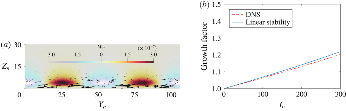
Transverse mode at
 $\unicode[STIX]{x1D6FC}=3^{\circ },~\unicode[STIX]{x1D6F1}_{s}=1.66$
: (a) disturbance flow vector field and normalised slope-normal velocity
 $w_{n}$
on the
 $y$
–
 $z$
plane. Slope flow is into the page; (b) temporal growth.

4.1 Transverse mode of instability
For the case with
 $\unicode[STIX]{x1D6FC}=3^{\circ },\unicode[STIX]{x1D6F1}_{s}=1.66$
and
 $Pr=0.71$
, a DNS is carried out over a domain with size
 $50l_{0}\times 106l_{0}\times 50l_{0}$
, where
 $l_{0}$
is the length scale defined in (2.6). The results confirm a stationary purely transverse instability, agreeing with the LSA and growth rate analysis in § 3.1. In figure 6(a), the instantaneous velocity disturbance profile projected onto a plane normal to the main velocity is shown. It can be seen that the normalised wavelength of the simulated instability is approximately
 $\unicode[STIX]{x1D706}_{n}=\unicode[STIX]{x1D706}_{y}/l_{0}\approx 18$
, corresponding to a normalised wave vector of
 $k_{y}=2\unicode[STIX]{x03C0}/\unicode[STIX]{x1D706}_{n}\approx 0.35$
. To measure the temporal growth of the instability, the growth factor
 $G(t)=\sqrt{\langle w^{2}\rangle (t)}/\sqrt{\langle w^{2}\rangle (t_{0})}$
for
 $t>t_{0}$
is introduced, defined as the spatial root-mean-squared vertical velocity normalised by the value at reference time
 $t_{0}$
. The simulated temporal growth of the instability is plotted alongside the growth rate predicted by linear stability theory for
 $k_{y}=0.35,\unicode[STIX]{x1D6F1}_{s}=1.66$
, as marked by point T in figure 3(a), which also corresponds to
 $[0,k_{y}]$
in figure 2(a). The non-dimensional growth rate from the DNS has a value of approximately
 $6.15\times 10^{-4}$
, closely agreeing with the value of
 $6.66\times 10^{-4}$
predicted via the linear stability theory.
4.2 Longitudinal mode of instability
For the case with the slope angle
 $\unicode[STIX]{x1D6FC}=66^{\circ }$
,
 $\unicode[STIX]{x1D6F1}_{s}=18.5$
and
 $Pr=0.71$
, a DNS is conducted on a domain with dimensions
 $50l_{0}\times 25l_{0}\times 50l_{0}$
. In agreement with the analysis in § 3.1, the simulation results show an oscillating instability propagating along the slope direction. Figure 7(a) displays the instantaneous disturbance velocity profile on a plane parallel to the base-flow direction and normal to the surface. It can be seen that the normalised wavelength of the simulated instability is approximately
 $\unicode[STIX]{x1D706}_{n}=\unicode[STIX]{x1D706}_{x}/l_{0}\approx 25$
, corresponding to a normalised wave vector of
 $k_{x}=2\unicode[STIX]{x03C0}/\unicode[STIX]{x1D706}_{n}\approx 0.25$
. The temporal growth of the instability is tracked by the same growth factor
 $G(t)$
used for the analysis of transverse instability. The simulated temporal growth of the instability is shown with the growth curve resulting from linear stability theory in figure 7(b). The non-dimensional growth rate from the simulation has a value of approximately
 $1.2\times 10^{-3}$
, in close agreement with the prediction from LSA for
 $k_{x}=0.25,\unicode[STIX]{x1D6F1}_{s}=18.5$
, highlighted with the marker L in figure 3(d), also visible as
 $[k_{x},0]$
on figure 2(b). According to LSA, the normalised frequency of the longitudinal instability for this particular set of parameters is approximately 0.115. The simulated instability has a normalised frequency of 0.125, which is close to the LSA results.
Longitudinal mode at
 $\unicode[STIX]{x1D6FC}=66^{\circ }$
,
 $\unicode[STIX]{x1D6F1}_{s}=18.5$
. (a) Disturbance flow-field vector and normalised slope-normal velocity
 $w_{n}$
on the
 $x$
–
 $z$
plane. Slope flow is from right to left; (b) temporal growth.

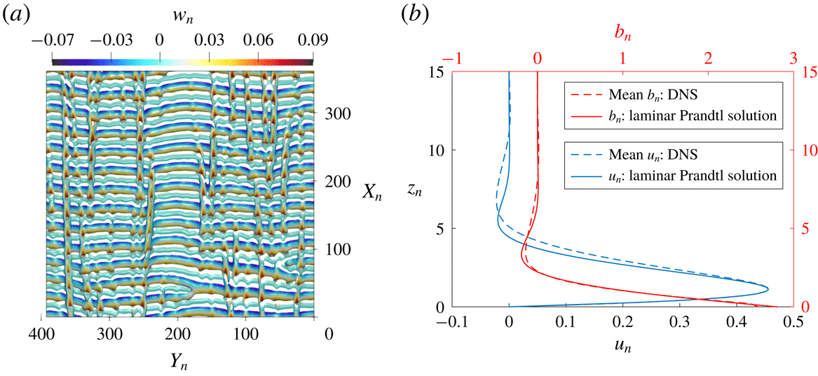
Mixed-mode instability at
 $\unicode[STIX]{x1D6FC}=66^{\circ },\unicode[STIX]{x1D6F1}_{s}=25$
. (a) Q-criterion contour visualisation of the instantaneous vorticity field, coloured by the normalised slope-normal velocity
 $w_{n}$
; (b) comparison of the normalised mean velocity and buoyancy profiles against the Prandtl solution.

4.3 Mixed mode of instability
For the case with
 $\unicode[STIX]{x1D6FC}=66^{\circ }$
as discussed previously, if the flow is subjected to more unstable conditions, i.e.
 $\unicode[STIX]{x1D6F1}_{s}$
is further increased beyond 20, then according to figure 4, both the transverse and longitudinal modes will become unstable. For subsequent discussions,
 $\unicode[STIX]{x1D6F1}_{s}$
is fixed at 25. Simulation for this case is carried out on a comparatively larger domain of
 $400l_{0}\times 400l_{0}\times 50l_{0}$
to capture multiple vortex rolls along all directions. Since, in this case, the horizontal dimensions of the simulation domain are an order of magnitude larger than the height, a less refined grid resolution is chosen for the along-slope and cross-slope directions than in the two previous cases such that there are approximately two grid points per length scale
 $l_{0}$
along these directions. An instantaneous snapshot of the full flow field is shown in figure 8(a). Here, the isocontour of the Q-criterion at 4 % of its maximal positive value is used for vortex identification (cf. Kolář Reference Kolář2007). Both longitudinal and transverse vorticity rolls are simultaneously present in the flow field, and are intricately interwoven with each other.
Figure 8(b) compares the spatiotemporally averaged velocity and buoyancy profiles from the simulated unstable flow field with the Prandtl’s solution with the same laminar flow parameters. The total averaging time window is roughly 30 times the flow-through-time based on the mean velocity at the jet tip. The comparison shows that at low altitudes, there is very little difference between the averaged unstable profile and the laminar Prandtl profile. At higher altitudes above the jet, however, the flow pattern is visibly altered; the mean velocity magnitude of the unstable flow decays more slowly with growing height than the laminar solution due to enhanced mixing caused by the instability. On the other hand, modification of the mean buoyancy field from the Prandtl profile is much weaker. As evident from the lack of small scales in figure 8(a), the flow is not turbulent but the mixed-mode instability is already influential in modifying Prandtl’s laminar velocity profile noticeably.
5 Conclusions
Despite its apparent simplicity, Prandtl’s katabatic slope flow model exhibits a surprisingly rich structure in linear response to small perturbations. It is prone to distinct instabilities governed by three dimensionless parameters, which are the Prandtl number, the slope angle, and a stratification perturbation parameter,
 $\unicode[STIX]{x1D6F1}_{s}$
, that we have introduced in the present work. For low to moderate slope angles, a three-dimensional, stationary transverse mode of instability is predicted to develop, even though Prandtl’s profile is a parallel flow; for steep slopes beyond
 $62^{\circ }$
, an oscillatory longitudinal instability is triggered instead due to the growing gravity component along the slope direction. At sufficiently small angles such that
 $\unicode[STIX]{x1D6FC}\lesssim 5^{\circ }$
, the transverse mode of instability can develop under conditions with implied Richardson number exceeding the critical value of 0.25 as stipulated by the Miles–Howard theorem. Thus, the Prandtl model for shallow slopes is an example of a parallel flow that does not satisfy the well-known
 $Ri>0.25$
condition for stability. The disagreement with the Miles–Howard theorem can be explained by the presence of viscous and heat conduction effects as well as misalignment of shear with stratification. For sufficiently high values of
 $\unicode[STIX]{x1D6F1}_{s}$
, both instabilities coexist, leading to an intricate pattern of crisscrossing vortex rolls.
An important implication of our current study is that, for a given fluid, linear stability of katabatic slope flows cannot simply be determined by a single dimensionless parameter alone, such as the Richardson number. Indeed, recently, a growing number of results have emerged to show that a single
 $Ri$
-criterion given by the Miles–Howard theorem is inadequate to reliably predict the onset of instability in stably stratified flows (e.g. Miller & Gage Reference Miller and Gage1972; Candelier et al.
Reference Candelier, Le Dizès and Millet2011; Kaminski, Caulfield & Taylor Reference Kaminski, Caulfield and Taylor2017). Our study adds to this existing pile of evidence by demonstrating that in the case of katabatic slope flows, slope inclination, background stratification as well as heat transfer rate at the surface are all important parameters governing the stability of the given flow configuration. Future prospective modelling and parameterisations of stably stratified flows on complex surfaces may benefit from considering this non-trivial dependence in their formulations.
Acknowledgements
Research was sponsored by the Army Research Office and was accomplished under Grant no. W911NF-17-1-0564 with Dr J. G. Baryzk as the programme manager. This research was supported in part by the University of Pittsburgh Center for Research Computing through the resources provided.