2.1 Fuzzy set theory

The motivation behind fuzzy set theory (Zadeh, Reference Zadeh1965) is the attempt to capture and handle analytically the notion of an object (e.g. a number, or a logical value) whose value is not sharply defined: e.g. “a bad winter”, “a large loss”, “a risky account”.

At the core of fuzzy set theory is the concept of fuzzy membership, a generalisation of the concept of membership to a set: in the “vanilla” version of set theory, an element x of a space Ω either belongs to a set A or it does not: the value of the membership function μ_A(x) is either 1 or 0. In fuzzy set theory, μ_A(x) can be any number between 0 and 1, e.g., we can say that losses of £10, £100k, £10m have membership 0, 0.5, 1 (respectively) to the set of large losses.

Fuzzy set operations (union, intersection…) can also be defined as a natural extension of the operations for standard set theory: e.g., the membership function of the union of two sets is the maximum of the membership functions of the two sets: .

Fuzzy numbers (as opposed to crisp numbers) can also be defined based on membership functions. In informal terms, a fuzzy number is a fuzzy subset of the real numbers whose membership function is centred on a given real number. A fuzzy arithmetic can then be created based on these fuzzy numbers. The essential tool for this is Zadeh's extension principle, which states that if * is a binary operation (e.g. sum, product…) and A, B are two fuzzy numbers, then the membership function for is

(1)

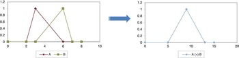
In the simple case of the sum of two triangular fuzzy numbers A and B, things work as in Figure 1. Much of the arithmetic of fuzzy numbers bears an obvious resemblance to interval arithmetic.

Figure 1

Sum of two fuzzy numbers A, B.

Moving a step forward, we can use Zadeh's extension principle to define crisp functions of fuzzy numbers:

(2)

Although the extension principle is simple when applied to monotonic functions and triangular fuzzy numbers, it becomes quickly unwieldy when applied to non-monotonic complex functions and to operations involving fuzzy numbers with complex membership functions. It is perhaps for this reason that (as far as the author is aware) a complete fuzzy calculus has never been developed.

A simple example of fuzzy numbers in non-life insurance is provided by the individual loss estimates for claims that have been reported but have not yet been settled. This will be a fuzzy number with lower limit equal to the amount paid that far and the higher limit equal to the policy limit, or a narrower range if the claim manager is confident about the possible outcome. The highest value of the membership function corresponds to the best estimate.

Fuzzy set theory has been explored at some length in the actuarial literature. The best known example is perhaps the paper by Cummins & Derrig (Reference Cummins and Derrig1997), “Fuzzy financial pricing of property-liability insurance”, which attempts to “fuzzify” the Myers-Cohn method for pricing general insurance contracts, according to which the price of a policy is set so that “the net present value of premiums is equal to the present value of the losses, expenses and federal income taxes incurred by the company as a result of issuing a particular policy”. The reader interested in a comprehensive overview of the applications of fuzzy set theory to insurance is referred to the paper by Shapiro (Reference Shapiro2004).

2.2 The Bayesian approach

In the Bayesian approach to modelling uncertainty, both uncertain data and soft/expert knowledge are also modelled as probability distributions. This approach is based on the Bayes theorem: Pr(θ | Z) = Pr(Z | θ) Pr(θ)/Pr(Z), which allows to calculate the posterior probability Pr(θ | Z) of θ (e.g., a parameter) conditional to Z (e.g., the data) as the probability Pr(Z | θ) of Z conditional to θ times the prior probability Pr(θ) of θ.

Formally, this is a straightforward consequence of the axioms of probability theory when using conditional probability, but the use of Pr(θ) to represent our initial beliefs on θ – rather than an objective state of things – has long been controversial (see for example Popper, Reference Popper1959). Despite this controversy, the Bayesian approach has gained more and more acceptance in recent decades, undoubtedly aided by the availability of larger computing resources that have made it possible to calculate posterior probabilities in complex situations.

Actuaries are familiar with the Bayesian formalism. For example, credibility theory, a standard tool of general insurance, can be framed in a Bayesian context: the information coming from the data is combined with that coming from an external source (which represents our prior knowledge), and the relative weight is determined by the balance of the variance of our data and the variance of the prior distribution.

In all but the simplest cases, there are many stages between the available data and the final results of a risk costing exercise. Prior knowledge and uncertainty are found at all stages: it is therefore important to be able to determine how uncertainty and beliefs are propagated across all stages of the methodology. Bayesian networks provide a way to do this. The most complete reference to Bayesian networks is probably the book by Pearl (Reference Pearl1988). A good, shorter (and simpler) introduction can however be found in the book by Russell & Norvig (2003), arguably the best introduction to artificial intelligence available.

Bayesian networks provide a way of representing a joint probability distribution, highlighting the dependency relationships between the variables. Formally they are directed, acyclic graphs, i.e. collections of nodes and arcs where each arc has a direction and there are no cycles:

• • Each node represents a random variable and has an associated quantitative probability information.

• • Two nodes A and B are connected by an arc from A (the parent node) to B (the descendant) if B is dependent on A.

The cornerstone for the construction of a Bayesian network is the so-called chain rule which gives the joint probability distribution as a function of the conditional probabilities:

(3)

To specify a Bayesian network, we need to identify which dependencies in Equation (3) (which is fully general) can be dispensed with, in order to make the network as compact as possible. Therefore we want to replace Equation (3) with the sparser

(4)

In Equation (4), parents(X_i) is the set of variables on which X_i actually depends directly. This suggests another view of Bayesian networks (alternative to that of a joint probability distribution) as a graph encoding a collection of conditional independence statements. This encoding is called a “topological semantics” and can be expressed by one of the following equivalent specifications:

• • a node is conditionally independent of its non-descendants given its parents;

• • a node is conditionally independent of all the other nodes in the network, given its Markov blanket (= parents, children, children's parents)

A conditional probability table (CPT) must be associated with each random variable: this provides the quantitative information of the dependency of a node on its parents.

An example of Bayesian network is provided in Figure 4.

2.3 A practical general insurance example: Determining the parameters of a severity distribution based on estimated losses and using expert knowledge

The differences between different methods to address uncertainty are better understood through a simple example. Suppose we are pricing some type of liability business and that there is a consensus that the proper model for doing so is a single parameter Pareto distribution with cumulative distribution .

The problem is calculating the parameter α of the Pareto distribution, based on:

• • loss estimates , which are known with uncertainty, and on

• • prior knowledge/beliefs about the parameter (e.g. a range of possible values for α)

In the case of crisp data and no prior knowledge available, one can use MLE for a point estimate of the parameter α: , and calculate the standard error through the Fisher information matrix (a single value, in this case) or the bootstrap.

When data uncertainty is present and expert knowledge is available, we need a mechanism that gives more weight to data points that are more certain (e.g. settled or almost settled claims) and that strikes a balance between what the data say and what the prior knowledge says. Let us see how this problem is solved using three different methodologies: a heuristic approach, fuzzy set theory, Bayesian networks.

For illustration purposes, we consider an actual numerical example. We have generated 50 losses from a (single-parameter) Pareto distribution with threshold x ₀ = £1m and α = 2.5. For each loss we have generated a random outstanding ratio (the amount yet to be paid) and we have applied distortions to each data point based on this outstanding ratio, reflecting the uncertainty on what the ultimate settlement will be, obtaining 31 losses in excess of £1m that are affected by uncertainty. We have then “forgotten” about how these figures were derived and we have tried to infer what the true value of α is. We have also assumed that prior knowledge/underwriting guidelines tell us that α should be in the interval [2,5].

Heuristic approach. Before looking at how fuzzy set theory and Bayesian analysis can help us, let us take a look at how this problem can be solved by using a heuristic approach, as actuaries will often make use of heuristic, sensible rules to deal with uncertainty.

One simple approach is as follows.

1. (i) Use MLE to find α _MLE and se(α _MLE) and parametric bootstrap to find the standard deviation σ _BS(α) of different estimates of α for variations due to data uncertainty. Basically, to calculate σ _BS(α) one needs to calculate α _MLE many times for different samples based on the initial data set. Unlike non-parametric bootstrap, each sample includes exactly the same losses but the value of each loss is drawn at random from a distribution centred around the best estimate and with a standard deviation proportional to the uncertainty on the loss.

2. (ii) Use a credibility approach to combine the above with underwriter's opinion: e.g., (subject to α* being between 2 and 5). In this expression, α _UW is the default value proposed by the underwriter, and . The quantity Var(α _UW) is the variance of the underwriter's estimate.

In the case of our numerical example, we have found α _MLE = 1.94, α _UV = 3.5, se(α _MLE) = 0.46, σ _BS(α) = 0.20. If we assume that Var(α _UW) = 0.25, this yields as our estimate of the Pareto parameter, roughly midway between our MLE estimate and the underwriter's prior guideline.

Despite the fact that this method does not have a solid theoretical foundation and many alternative solutions are possible, some of the methods that reinsurers use in practice are not too dissimilar from that above.

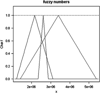
Using fuzzy set theory. Each non-settled loss X_i can be represented as a triangular fuzzy number , with width larger for losses that have a large outstanding percentage. Figure 2 shows examples of some of the 31 actual losses.

Figure 2

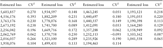
Some of the losses in Table 1, represented as triangular fuzzy numbers. The calculations and graphics of this section have been performed with the R package “fuzzyOP” by Semagul et al. (Reference Semagul, Altindas, Macit, Umar and Unal2009).

Fuzzy arithmetic can be used to produce an MLE-like estimate of the parametersFootnote 1. E.g., for a Pareto distribution, we can use the equation . As the logarithm is a monotonic function, it is easy to obtain the membership function of ln x_j for all losses x_j using Equation (1). The membership function of can then be obtained through Equation (2). Since the denominator is positive by definition (all x_j's are greater than x ₀)), is a well-defined fuzzy number with finite support. The width of this support (and actually the overall shape of the membership function) is related to the uncertainty on α. Notice that this does not necessarily decrease as n→∞ (see discussion in Section 2.5).

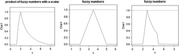
The overall result is a fuzzy number , whose shape can be seen in Figure 3 (left).

Figure 3

Left: fuzzy number resulting from the calculation of Equation . Centre: fuzzy number representing the prior knowledge on α (or the underwriting guidelines). Right: fuzzy number representing the final estimate of α, obtained as the intersection of the membership functions at the left and the centre.

Prior knowledge can be incorporated by representing the parameter as another fuzzy number with membership function . In this experiment we have modelled the prior knowledge as a triangular number between 2 and 5, centered at 3.5, as in Figure 3 (centre).

The final result can be obtained as the fuzzy intersection of the two estimates:

(5)

and is shown in Figure 3 (right).

The choice of the intersection seems to make sense as it requires that both constraints (those coming from data and that coming from the soft knowledge) be satisfied at the same time.

One computational complication of the procedure is the fact that the membership function becomes more and more complex. Also, it is not clear how to extend this procedure to a case when we have a more complex distribution for which the ML solution is not analytical, e.g. with a GPD.

Using Bayesian networks. In a probability context, each non-settled loss can be represented by a probability distribution centred on the best estimate of the incurred amount. The dispersion of the distribution will be related to the uncertainty regarding the loss, and this in turn depends on a number of factors, such as the outstanding ratio (outstanding amount divided by incurred amount), the size of the loss, the opinion of the claims manager on the possible variability, the age of the loss, etc.

Prior knowledge on the parameters can be incorporated by a prior distribution on the parameters themselves.

In the case where there is prior knowledge on the parameters but no data uncertainty, an estimate of the parameters θ can be obtained by maximising the posterior probability of θ given the data, . If there is no prior knowledge, i.e. is the non-informative prior, the term can be dropped and the problem reduces to standard maximum likelihood estimation.

Now consider the case where there is data uncertainty as well as prior knowledge: in this case the input is given by the loss estimates . For each estimate we may have some additional information , including, e.g., the outstanding ratio, the loss date, the type of injury, etc.). (For the sake of notational clarity the dependency on these variables is hidden in the equations below.)

This problem lends itself quite naturally to the formalism of Bayesian networks. This makes use of the following standard equation:

(6)

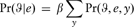
where represents the query variables (in our case: the parameter(s) of the severity distribution), e is a realisation of E, representing the evidence variables (in our case: the estimated loss amounts), y is a realisation of Y, the hidden variables (in our case: the true loss amounts). Note that all of these quantities should be interpreted as vectorial random variables.

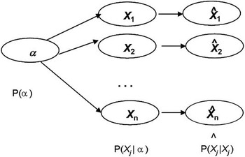
Equation (6) relates the posterior distribution , which is the quantity we want to maximise, with the joint distribution , which can be represented as a Bayesian network (see Section 2.2). There are many ways to specify a Bayesian network: one which usually leads to a compact representation is the causal model, where nodes representing causes are added first and nodes representing symptoms are added later. In our example, a simple causal representation is as shown in Figure 4.

Some structural simplifications have been made in the model of Figure 4, by assuming that:

1. 1. the variables (estimated losses) depend on α only through the variables (true losses);

2. 2. does not depend on if ;

3. 3. all are independent of one another given α (a common assumption).

It is always critical to decide which variables can be considered to be independent of the others. In most real-world cases, there is always an argument for objecting to the claim that two given variables are independent. Bayesian networks help introduce some discipline in this: every added link increases the complexity of the network and therefore makes inference harder, so new links should be added only if the growth in complexity is justified by the gain in accuracy. In practice, this means that one often gets rid of tenuous links (see discussion on compactness and node ordering in Russell & Norvig, 2003). In our example, it should be noted that Assumption 2 above is only a rough approximation.

The Bayesian network of Figure 4 corresponds to the following representation of the joint distribution:

After some algebraic manipulations and the application of Bayes’ rule, we obtain

(7)

Figure 4

A Bayesian network representing a severity distribution with some prior knowledge on the parameters (α) and uncertainty on the loss amounts.

Despite the complex form of this equation, its right-hand side is a function of the parameter(s) α, which we can maximise by numerical methods. In our case α is a single parameter (rather than a vector of parameters), the exponent of a Pareto distribution, and the posterior probability can therefore be maximised very efficiently. The three functions we need to know to calculate the integrals in Equation (7) are:

• • the conditional probability , which for a Pareto distribution is ;

• • the prior probability . This should reflect our prior knowledge on the parameters. Here we have assumed a Beta distribution , and a = b = 6. This constrains α to be between 2 and 5 and sets the mean at 3.5. The value of a will drive the width of the Beta distribution (the large a is, the narrower the distribution);

• • the conditional distribution , or rather – to use the complete notation – . This is the IBNER distribution, and will normally be informed by the actual reserving experience. For simplicity, let us assume here that the IBNER distribution is a Gaussian distribution: , with , where the coefficient of variation is estimated based on the actual data. This approach is usually called empirical Bayesian approach, as the prior distribution is actually estimated based on some previous, or external, experience, rather than made up from scratch.

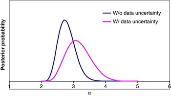
By substituting these probabilities into Equation (7), we obtain the posterior distribution of α which we can then maximise – a simple one-dimensional numerical optimisation problem. The (numerically obtained) posterior distribution – with and without data uncertainty – is shown in Figure 5.

Figure 5

The posterior distribution for α for our example dataset, with and without data uncertainty. Notice that the distribution with data uncertainty is wider and is also closer to the underwriter's guideline α = 3.5, probably because data uncertainty generally increases the uncertainty on the parameter calculated from the data and therefore puts more weight on the prior.

2.4 Another practical general insurance example: Model uncertainty

Model uncertainty is a particularly thorny issue as the problem of quantifying model uncertainty is as difficult as that of determining what the correct model is. There is a dumbed-down version of this problem, however, which seems to be more approachable: this is the case where there is only a finite number of competing models available, and we want to select the one that is better at predicting the results on an independent sample. In the example of Section 2.3, we might be undecided as to whether to model our losses with a Pareto (fat-tail) or an exponential (thin-tail) distribution, and we want our data to guide us in choosing between these two alternatives only. The general idea is to assign to each model a prior probability and calculate the posterior probability of the model given the data. This is explored for example in Bishop (Reference Bishop2007).

The main idea is to compare a set of L models where . Each model is a probability distribution, e.g. the probability distribution of losses. Each model has a prior probability . Given a training set , we are interested in evaluating the posterior distribution:

(8)

In the equation above, the term expresses a prior preference for different models, whereas the term expresses the preference shown by the data themselves for different models, and is called the model evidence. Equation (8) can be used to select the best among a number of competing models.

In our case, we might have a preference for Pareto, because (for example) for 70% of our large clients the Pareto distribution turned out to be more successful in fitting our data. Therefore we might assign a 70% prior probability to the Pareto model and a 30% probability to the Exponential model. Again, this can be considered an empirical Bayesian approach. The posterior probability of the Pareto distribution is now given by:

(9)

and if this is larger than 0.5 we may choose a Pareto model (as opposed to an exponential) for modelling our data.

2.5 Comparing the fuzzy set theory and the Bayesian approaches to uncertainty

Several authors have compared the probabilistic and the fuzzy logic approach to uncertainty. One well-known example is the lively debate around the paper by Elkan (Reference Elkan1994), which was about alleged inconsistencies in fuzzy logic and whether other paradigms are more adequate to replicate human reasoning (see, e.g., de Silva & Attikiouzel, Reference de Silva and Attikiouzel1994). The debate has spread to the actuarial community (Cummins & Derrig, Reference Cummins and Derrig1997). Table 1

Table 1

A sample of 31 losses randomly drawn from a single-parameter Pareto, which will be used to illustrate the different approaches to uncertainty. The uncertainty on each loss is expressed as a coefficient of variation (squared). For this particular data set, the maximum likelihood estimate of the parameter α is 1.94 (therefore lower than the ‘real’ value α = 2.5). The standard error on the parameter can be calculated by standard MLE tools and turns out to be α = 0.35.

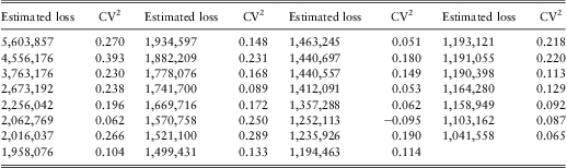
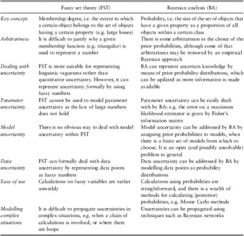
We here list some of the most contentious issues, and we summarise these points and the points that emerged in the previous sections, in Table 2.

Table 2

A comparison of the fuzzy set theory and the Bayesian approaches to uncertainty.

The wrong type of uncertainty? The most common criticism of fuzzy set theory is probably that it is nothing but an unwieldy version of probability theory, and that everything that can be dealt with by fuzzy set theory can also be dealt with by Bayesian probability. When it comes to representing numbers, membership functions look very much like distribution probabilities indeed – so why not just use those? The classical response to this is that fuzzy set theory captures fuzzy membership to a set, whereas probability distributions aim at calculating the likelihood that an element belongs to a set in a crisp way. The conceptual difference is important: when we say that a loss is “large”, we are using a fuzzy concept. No uncertainty is involved here – the loss may be exactly £130,000 and may have already been settled – but whether this loss belongs to the set of large losses is indeed fuzzy (and context-dependent). The author's view on this debate is that although there is no question that fuzzy set theory and probability theory are two conceptually distinct disciplines, each modelling different aspects of uncertainty, the interest of fuzzy set theory seems to be mostly logical and linguistic. The type of uncertainty we are concerned with in insurance is not of a linguistic kind: we may not be able to define crisply what a “large” loss is, but there is hardly a business case for attempting it! We are concerned with uncertainties on the amounts, not with semantic uncertainty. In all the applications of fuzzy set theory in the actuarial literature known to the author it is this second type of uncertainty which is addressed – this is the case, for example, in Cummins & Derrig (Reference Cummins and Derrig1997), where fuzzy logic is used to quantify the uncertainty on the risk-adjusted discount rate for losses, on the losses themselves, on the premiums, etc. In all these cases, fuzzy logic provides a formalism which produces reasonable results, but there is no reason why a richer probabilistic framework could not be used in its stead.

Is fuzzy set theory unwieldy? One of the main reasons of the recent success of Bayesian analysis lies in the fact that many tools have been developed for the calculation of posterior distributions: these include Markov Chain Monte Carlo techniques, Gibbs sampling, Metropolis-Hastings (see, e.g., Mackay (Reference MacKay2003) or Roberts & Casella (Reference Roberts and Casella2004) for a review of these methods), and all the techniques applicable to Bayesian networks to take advantage of their sparsity. On the other hand, anything beyond simple arithmetic is painful with fuzzy set theory. Until a proper calculus is developed, only elementary applications to general insurance will be possible.

Parameter uncertainty. Another issue with fuzzy set theory is that it deals poorly with parameter uncertainty. As observed for example in Nikolaidis et al. (Reference Nikolaidis, Cudney and Chen1999), the law of large numbers does not hold for fuzzy numbers. The average of n fuzzy numbers with the same membership function has exactly the same membership function of the component numbers, regardless of n. On the contrary, in a probabilistic setting the average of n independent numbers will have a narrower distribution than its components, and this narrowing can be quantified by the central limit theorem. This leads to the apparent paradox that adding more information does not lead to a reduction in uncertainty in fuzzy set theory! The sum of fuzzy numbers can therefore be likened to the sum of perfectly correlated variables.

Model uncertainty. There is no obvious way by which fuzzy set theory can deal with model uncertainty. In Cummins & Derrig (Reference Cummins and Derrig1997), one of the stated reasons to use fuzzy set theory was actually that there is uncertainty as to whether capital asset pricing model is the correct model to produce a risk-adjusted discount rate for losses, r_L (see Cummins & Derrig (Reference Cummins and Derrig1997), Section 2.3). However, this fact is only used to justify an additional uncertainty on the result of this model – r_L itself. In other words, this model uncertainty is translated into a sort of parameter uncertainty. On the contrary, Bayesian theory incorporates model uncertainty by using the prior probability on models, and gives a recipe on how to choose between a number of competing models. It is a limited solution but it is further-reaching than anything one can do with fuzzy set theory.

Other issues. As discussed, e.g., in Bender (Reference Bender1996), it is tricky to use fuzzy set theory when multiple levels of operations and decisions must be made. Furthermore, some of the basic definitions of fuzzy set theory, such as the definition of intersection, lead to counterintuitive results and may need ad hoc amendments for specific applications (Lemaire, Reference Lemaire1990).

3.1 Probabilistic temporal models

Temporal aspects are usually addressed in computational intelligence by using a probabilistic temporal model (also known as a state-space model).

A probabilistic temporal model requires three ingredients:

1. i. A transition model. This is the conditional distribution , and fully describes time evolution in the case of first-order Markov processes.

2. ii. A sensor model (aka observation model). This is the probability , describing how the evidence is affected by the state of the world. We assume that the evidence only depends on the current state (Markov property of evidence), i.e. . The state of the world is supposed to be “hidden”, that is, measurable only through the observation model.

3. iii. A prior probability. This is the probability over the states at time zero.

Notice that the transition and the observation model themselves must often be learned from observations.

The probabilistic model above immediately sheds some light on the notion of time dependence, and it allows us to define different levels of stationarity in terms of the transition model (note that the time t in the following relations is discrete):

• • a static system is one where the state of the system does not change:

• • a stationary system is one where does not itself depend on t, that is, for all k;

• • a non-stationary system is one where depends on t, that is, , where the distribution is often not known. In this case, if the time dependence is “slow”, it may still be possible to model the system as locally linear (or constant) with slowly changing parameters;

• • the worst case of all is of course the one where events at different times are completely independent of each other: . In this case prediction is, by definition, impossible. A conceptually different but practically similar case is that in which there exists some dependency but the distribution changes so quickly that the past experience becomes almost immediately irrelevant for prediction purposes.

Many results of probabilistic temporal models assume that the system is stationary and has the Markov property of evidence. However, they can usually be extended at least to the case where the system is quasi-stationary (i.e., it changes slowly).

The ingredients of the probabilistic temporal model can be combined to specify the whole joint distribution:

(10)

The temporal model above allows to solve several different inference problems, including (list borrowed from Russell & Norvig, 2003):

• • The filtering problem: i.e., calculating the belief state (the posterior distribution may represent the number of losses expected in year t given all claims reported up to t (a non-trivial problem when IBNR claims are a significant portion of the total claims);

• • The prediction problem: i.e., calculating the posterior distribution of a future state given the evidence until now, . A typical example is experience rating – the calculation of the future distribution of claims given historical losses. Note that prediction can be seen as filtering without the benefit of new evidence.

• • The smoothing problem: i.e., calculating the posterior distribution of a past state given all evidence up to the present, . A classical example is reserving, where we need to keep updating our estimate of losses in year k for many years after that – until we are fully sure that no more claims can be reported for that period.

The solution to any of these problems usually comes in the form of a recursive equation, with a repeated application of the Bayes’ rule and of the Markov property of evidence. As an example, the recursive equation for filtering can be written as:

(11)

The recursive equation for prediction is instead:

(12)

so that prediction can be seen as filtering without the benefit of new evidence.

We now look at different examples of temporal probabilistic models: hidden Markov models, Kalman filtering and dynamic Bayesian networks.

3.2 Hidden Markov models (HMMs)

A hidden Markov model (HMM) is a temporal probabilistic model, in which the state of the process is described by a single discrete random variable (possibly, a vector variable). This representation allows “a simple and elegant matrix implementation” of the generic model (Russell & Norvig, 2003). In the equations below it is assumed that the system is Markov and stationary. As usual, the results can easily be extended to the quasi-stationary case.

The transition model is represented as

The sensor model is represented as the diagonal matrix whose diagonal elements are given by the values of .

The updating equation is

where is the so-called “forward message”.

3.3 Kalman filtering

Kalman filtering is a type of regression analysis enhanced with a mechanism for updating the regression parameters, which are assumed to evolve in time. A classical application of Kalman filtering is radar tracking: once an object is identified at time t, its position at time t + Δ is determined by combining the noisy observation at time t + Δ with an assumption on where the object is expected to be found at time t + Δ based on its position at time t.

Although various extensions of the Kalman filter can be found in the literature, the standard model of Kalman filtering requires the system to have the Markov property of evidence and to be stationary: furthermore, it is assumed that the current state follows a multivariate Gaussian distribution. The transition model for the Kalman filter is therefore , where F and Σ_x are matrices describing the linear transition model and transition noise covariance. The sensor model is , where H and Σ_z are matrices describing the linear sensor model and sensor noise covariance.

The update equation for the mean is now:

(13)

and the update equation for the covariance is:

(14)

where K_{t + 1} (the Kalman gain) is given by:

(15)

Equations (13), (14) and (15) are horrible to behold, but a few moments’ look at them will remind the actuary of credibility theory: the Kalman gain is the credibility given to the new observation , relative to the predicted state at time t + 1, .

As mentioned at the beginning of this section, the standard model, which is Markov, stationary and with a Gaussian transition and sensor model, has been extended in several directions.

• • The extended Kalman filter (EKF) incorporates non-linearities by only requiring that the model is locally linear. In practice, this means that the system is only locally stationary (Zarchan & Musoff, Reference Zarchan and Musoff2005; Ribeiro, Reference Ribeiro2004). This works well for smooth, well-behaved systems – that is, systems that do not have abrupt changes;

• • The switching Kalman filter, which attempts to model strongly non-linear behaviour such as obstacle avoidance by using multiple Kalman filters among which it is possible to switch (Ghahramani & Hinton, Reference Ghahramani and Hinton1998; Hamilton, Reference Hamilton1989).

Both cases above are special cases of dynamic Bayesian networks, that provide a far more general solution to the problems addressed by the Kalman filter.

3.4 Dynamic Bayesian networks (DBNs)

Dynamic Bayesian networks are Bayesian networks representing temporal models. They are completely general in the sense that they do not add any further assumptions to those of general temporal models.

The joint probability distribution of Equation (10) already provides a full specification of a DBN, as it clarifies the dependency structure of the network. This can be rendered graphically as in Figure 6, both in the rolled-up (recursive) version and in the unrolled version. The term “unrolling” refers to the development of the recursion.

Figure 6

A dynamic Bayesian network, in recursive (left) and unrolled (right) form.

The reason why the recursive formulation is important is that it allows to store the whole probabilistic model in constant space (the network does not grow with time) and update the network in constant time. The recursive formulation is equivalent to the unrolled one only if the system is stationary.

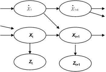
The Kalman filter is a special case of a DBN. This is illustrated in Figure 7, where a classical Kalman filter is shown as a rolled-up DBN.

Figure 7

Representation of a classical Kalman filter where both the position (x_t) and the speed (x_t) of an object are tracked as a dynamic Bayesian network are shown.

3.5 Practical general insurance example: Reserving

A pioneering application of probabilistic temporal models to general insurance is that of De Jong & Zehnwirth (Reference De Jong and Zehnwirth1983) in their work on reserving. The general case is quite complex so for illustrative purposes we will focus on the simple example that can be found in Section 5 of their paper.

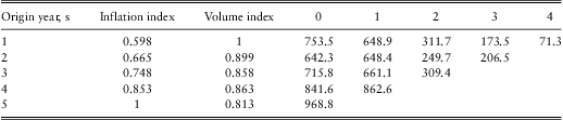
This is based on the run-off triangle in Table 3 (borrowed from De Jong & Zehnwirth, Reference De Jong and Zehnwirth1983), that gives the amount paid for each development year and for each origin year, taking into account some measure of inflation (the inflation index) and of exposure (the volume index).

Table 3

Example of a run-off triangle. The amounts in the triangle represent the incremental paid amounts for each origin year and for each development year (0 to 4). Amounts shown are in £1,000.

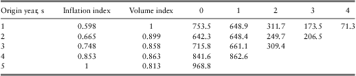
In this example, the observation (evidence) variables z_t are the successive diagonals of the paid triangle, as they represent the evidence collected in the latest calendar year. In the example above,

z ₁ = (753.5)^T

z ₂ = (642.3, 648.9)^T

z ₃ = (715.8, 648.4, 311.7)^T

z ₄ = (841.6, 661.1, 249.6, 173.5)^T

z ₅ = (968.8, 862.6, 309.4, 206.5, 71.3)^T

The underlying parameters are in this simple case the ultimate incurred claims x_s for each origin year s.

The observation equation, which connects the paid amounts to the ultimate claims x_s is (in this extremely simplified model):

where is a zero-mean random noise; is the expected value of payments for origin year t−d and development year d, which is decreasing monotonically as a function of the development year; is the exposure index for origin year t−d; λ_t is the inflation index for calendar year t;

The transition model is given by the simple random walk model:

where is again a zero-mean random noise.

We also need an initial state x ₀ corresponding to the unobserved origin year s = 0.

In De Jong & Zehnwirth (Reference De Jong and Zehnwirth1983), this problem is approached by using extended Kalman filtering, with the structural parameters varying with time and therefore indicated below as F(t), etc. The list below explains what these parameters look like in this simple case:

• • the matrix F(t) is a matrix with zeros everywhere except at elements where its value is 1;

• • the matrix is written as where is a t × 1 matrix whose only non-zero element is (1, 1) which can be set to 1, and was estimated by MLE methods as ;

• • the initial state x ₀ corresponding to origin year s = 0 and its covariance matrix Σ ₀ are back-calculated with MLE methods assuming that a number of diagonals are already given, obtaining the values x ₀ = 1146.3 and Σ ₀ = 2667.3;

• • the covariance matrix is a diagonal matrix whose diagonal values are the first t values from

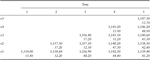
Kalman's update rules (Equations (13), (14), (15)) are then used to produce the projected values of the claims triangle. The estimates for the states xt generated by the Kalman filter are shown in Table 4:

Table 4

The estimates of the states x_t at different times. The quantities shown in italic and smaller case are the standard errors.

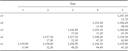
Kalman's update rules (Equations (13), (14), (15)) are then used to produce the projected values of the claims triangle. The structural parameters (F, H…) vary slowly with time and therefore this can be regarded as an application of the Extended Kalman Filter (EKF).

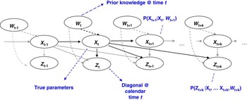
The results obtained in De Jong & Zehnwirth (Reference De Jong and Zehnwirth1983) could also be obtained by a dynamic Bayesian network like that in Figure 8. The model can be enhanced by adding nodes which represent (possibly discrete) random variables W_t incorporating prior knowledge on the things that might have an impact on the general level of claims for a given origin year (e.g. a bad winter) or on the amounts paid from a given year on (for example, new legislation on court awards for bodily injury liability). The transition model and the sensor model including these additional variables need not be linear or Gaussian.

Figure 8

A dynamic Bayesian network for loss reserving. The example in De Jong & Zehnwirth (Reference De Jong and Zehnwirth1983) does not require the variables W_t depicting prior knowledge, which are therefore connected to the rest of the network with dashed lines. All the edges except those to and from X_t are grayed.

Note that the model shown in Figure 8 requires some rearrangement before being cast as a standard transition/sensor model, since (k is the maximum number of development periods such that the hidden variables X_t are relevant to the evidence variables. In other words, we can assume that , where Ω_t denotes the collection of all other variables). Note that, as long as k is finite, this process can always be transformed into a first-order Markov process by a suitable redefinition of variables.

3.6 Comparison of different methods for temporal reasoning

In the previous sections we have looked at probabilistic reasoning over time, and at some specific models for dealing with it. We here summarise the advantages and disadvantages of the different methods:

• • Kalman filtering crucially depend on the assumption that both the sensor (observation) model and the transition model are linear multivariate Gaussian. Although the model can be extended into different directions (EKF, switching Kalman filter), the Kalman filter is simply not general enough to model all interesting situations in general insurance. In the practical case we looked at (reserving), many of the most relevant uncertainties over time depend on factors that are strongly non-linear and non-Gaussian, such as future changes of legislation, future changes in the reserving guidelines, sudden change in the riskiness of an account, etc. Some (although not all) of these non-linearities can be incorporated in a general probabilistic model, but it is awkward to address them with Kalman filters;

• • dynamic Bayesian networks are a more powerful method than Kalman filters:

  • ○ all Kalman filters can be represented as dynamic Bayesian networks or as hidden Markov models, but not vice versa;

  • ○ serious non-linearities can be addressed by dynamic Bayesian networks with both discrete and continuous variables;

  • ○ numerical methods such as Markov Chain Monte Carlo can be used for approximate inference in dynamic Bayesian networks;

• • hidden Markov models and dynamic Bayesian networks are equivalent formulations in the discrete case – however, dynamic Bayesian networks are more compact and allow gains from the sparsity of the connections between the random variables.

It should be stressed that all temporal models as we have presented them here have some limitations. In all cases, a prior model of the possible future changes is needed. This can be linear, or locally linear, or allow for strong non-linearities, but in all cases the information we have on the transition model is crucial. If changes too quickly, prediction is impossible and all we can do is rely on the very latest data. In practice, it is seldom the case that the past is completely irrelevant to the future, but there are times where the rules of the game change quickly and our ability to model future changes is very limited.

4.1 Individual agents and the environment

Each risk agent is assumed to be autonomous and to incorporate strategies to interact with the environment. The type of environment in which the agent moves is crucial. An environment can be (see Russell & Norvig, 2003; Wooldridge, Reference Wooldridge2001):

Fully v partially observable. A fully observable environment is simply one in which the agent always knows where it is. In the insurance world we usually have partially observable environments as we do not usually know for sure what our true underlying financial position really is (this is perhaps clearer in the case of long-tail business, where it takes a long time for the financial position of a given underwriting year to become finalised).

Deterministic v stochastic. A deterministic environment is one where the outcome of our actions is known for sure (in terms of the state the agent will be in). This is never the case in insurance: once for example we set the price of one policy we cannot know for sure what the volume sold and the claims to be paid will be.

Static v dynamic. A static environment is simply one that does not change with time, except for the actions of the agent. A dynamic environment has other processes operating in it, and these change the environment in ways that the agent cannot control. Needless to say, the insurance environment is highly dynamic. However, in some cases it may be necessary, or convenient, to assume that the environment does not change in the short term.

Discrete v continuous. A discrete environment is one with a fixed, finite number of states and of actions that can be performed. Again, the type of environments we are interested in are continuous. However, this distinction is not crucial, as we can usually approximate continuous environments with discrete ones.

Finally, note that the term “environment” may be misleading, as in insurance we normally mean it to encompass the context where an insurance company operates: its competitors, the judicial climate, the regulation, etc. However, the meaning in which we use it here is broader, and includes everything that affects the financial results and that is not determined directly by the actions of the agent. Specifically, it includes the distribution of losses.

4.2 Markov decision processes

Although there is no such thing as a fully observable environment in general insurance, it is useful to start considering this type of environment, because it prepares the ground for dealing with partially observable environments.

In this section we therefore assume that the environment is fully observable, stochastic, static and discrete. In our example, we are basically assuming that R-Age is so good at pricing that it is able to determine the parameters of the loss distribution with infinite accuracy. It is also so market-wise that it knows the demand curve for that policy with infinite accuracy, so that it knows exactly what the volume sold will be for a given price. However, underwriters at R-Age fall short of omniscience as they cannot predict the actual losses which will be incurred next year – only the distribution from which they are drawn.

This situation can be modelled by a Markov decision process, which is defined by:

• • An initial state S ₀

• • A Markovian transition model : at each time t, an agent will be in state s and will be able to perform an action a. As a consequence, it will move to state s′ with probability . The transition model is Markovian in the sense that the probability of reaching from s is assumed only to depend on s and not on the states that precede s.

• • A reward function R(s), establishing the reward received by the agent in state s.

How is this relevant to R-Age? The state s in which R-Age is at time t may be simply defined as a pair where C_t is the capital available and V_t is the volume sold at time t. Time is discretised and is in years. The initial state is the initial capital C ₀ and the initial volume V ₀. Actions are simply decisions on prices: therefore a is another symbol for P_t, the price charged at time t. The transition probability is the probability that if the price is set to a the capital will become C_{t + 1} (the volume V_{t +1} is deterministic in this simplified setting), and will depend exclusively on the aggregate losses incurred between t and t + 1 (for simplicity, we assume that these include expenses):

(16)

If we know the distribution of (e.g., a lognormal distribution) we know the distribution for C_{t + 1} given C_t and P_t: that is, the transition probability .

Equation (16) also allows us to define the reward for each state as:

(17)

which is simply the profit during year t.

Having defined what a Markov decision process is, we need a method to decide how good a strategy σ (i.e., a prescription specifying what the agent should do in any state it might reach) is. σ(s) is the action prescribed for the agent when this is in state s. We therefore need an ordering on the set of strategies – a utility function. Given the stochastic nature of the environment, the quality of a strategy σ is measured by its expected utility, where the expectation is calculated over all possible environment histories generated by σ. The term “histories” might be a bit misleading here, as it is used differently from normal actuarial practice: by environment history we mean in this context a sequence of future states.

An optimal strategy is thus one that achieves the highest expected utility. Interestingly, if the utility function is constructed wisely, strategies which yield high rewards in the short-term but are too risky will be penalised. As a result, there is a familiar balance to be struck between risk and reward, and this arises simply as a consequence of the stochastic nature of the problem: “the careful balancing of risk and reward is a characteristic of MDPs that does not arise in deterministic search problems; moreover, it is a characteristic of many real-world decision problems” (Russell & Norvig, 2003).

How can we assign a utility function to environment histories ? This depends, first of all, on whether the horizon for decision-making is finite (only rewards accumulated up to year N are relevant) or infinite (the whole future history is relevant). Finite horizon problems are more complicated because they are inherently non-stationary: the optimal decision will depend on how close you are to the deadline. We will assume that

• • the horizon is infinite – which simply means in our case that one does not know a priori how long one is going to stay in business;

• • the agent's preferences between state sequences are stationary, meaning that if the utility of is greater than that of , then the utility of is greater than that of .

It can be shown that under these conditions there is only one way in which we can assign utilities to sequences:

(18)

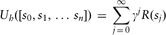
where γ, the discount factor, is a number between 0 and 1. The choice γ = 1 is usually not acceptable as it leads to infinite utilities.

Note that without ever mentioning the time value of money and without any other actuarial consideration, but simply assuming an infinite horizon and the stationarity of the agent's preference over state sequences, we have found that the only sensible way in which we can define utility is as the sum of the present value of future rewards!

We are now in a position to define the optimal strategy σ as the one which maximises the expected utility as defined in Equation (18):

(19)

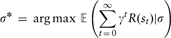
In the case of R-Age, the utility is simply the present value of future profits. As to what discount factor γ to use, that is a usual problem – in a normal situation, one solution is using the return expected by investors for the level of riskiness of this company (in this case, this policy). In the specific case addressed in this section – for which the only real uncertainty is in the randomness of the aggregate losses, whose parameters are assumed to be known with certainty – it would probably be more appropriate to choose a lower discount rate, such as the risk-free discount rate plus a “premium” related to, say, the coefficient of variation of the aggregate loss distribution.

How do we solve Equation (19)? The utilities of states are the unique solutions of the so-called Bellman equation, which relates the utility of one state s to the discounted utility of the state of its neighbours’ s′:

(20)

The Bellman equations (one for each state) can be solved iteratively, by starting with an arbitrary value of the utilities and then updating the utilities with this equation, called a Bellman update:

(21)

It can be easily shown that this iteration, which has the form , is a contraction in the space of the utility vectors, and has therefore a unique fixed point, to which the iteration ultimately converges. The speed of the convergence is related to the value of γ: as one would expect, the smaller γ is, the quicker the algorithm converges to the solution (see Russell & Norvig (2003), Section 17.2, for a more detailed discussion of the algorithm).

The discussion above applies to the case where the number of states is finite. This is not the case of R-Age, because the premium of a policy can be any number. However, the real world case can be approximated with a scenario involving a finite number of states.

A more important issue is the assumption that the environment be fully observable. As we will see in the next section, this is not a satisfactory assumption, and to address this case we need the more advanced formalism of partially observable MDPs.

4.3 Partially observable Markov decision processes (POMDP)

In practice, R-Age will not be able to determine its state : e.g., when writing long-tail business some claims will only be known or settled many years after their occurrence. The estimate of the current capital depends on the reserve estimates, which are uncertain (owing to IBNR, IBNER, etc). As a consequence, the true underlying financial position of the company is not known with certainty. Furthermore, the transition matrix will be uncertain, as the loss distribution is built upon a finite set of observationsFootnote 2.

In the language of intelligent agents we say that the environment is not fully observable and the agent does not know for certain which state it is in. This can be modelled by the so-called partially observable MDPs, or POMDPs (“pom-dee-pees”).

A POMDP requires the following ingredients:

• • A transition model T(s,a,s′)

• • A reward function R(s)

• • An observation model O(s,o) that specifies the probability of perceiving the observation o in state s

• • A belief state, i.e. a mapping between actual states s and the probability b(s) assigned to each of them. The belief state can also be defined as the posterior distribution over the current state, given all evidence to date: or, using the notation of our section on temporal models, .

As new observations are made, the belief state is updated, according to this equation, which is simply an application of Bayes’ theorem, with a non-standard format.

(22)

which can be abbreviated as

(23)

What makes POMDPs work is that the optimal strategy σ* depends only on the agent's current belief state and not on the state it is in. This is how a POMDP makes decisions:

POMDP decision process

1. 1. Given the current belief state (the optimal strategy given the belief state)

2. 2. Receive observation O

3. 3. Set the current belief state to and repeat

Interestingly, the problem of solving a POMDP on a physical state space can be reduced to that of solving an MDP on the corresponding belief state space:

• • The probability of reaching is

(24)

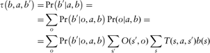
where , 0 otherwise.

• • The reward for belief state b can be defined as:

(25)

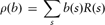
(that is, the reward for a belief state is the expected value of the reward for individual states)

These equations have the same form as the definition for fully observable MDPs (Section 4.2), the only difference being that the state s is replaced by the belief state . We have thus reduced the problem of solving POMDPs in the state space to the problem of solving MDPs in the belief space. It can be shown that an optimal strategy for this MDP is an optimal strategy for the original POMDP.

The difficulty, however, is that the space of belief states is continuous and usually high-dimensional. Solutions for this case have been developed as well, but their computational complexity becomes rapidly prohibitive as we increase the number of states: the problem falls in the class of PSPACE-hard problems, which are widely thought to require exponential time to solve (Papadimitriou, Reference Papadimitriou1994). Luckily, approximate methods for solving POMDPs have been developed, making use of the so-called “dynamic decision networks” (DDNs), which we will describe in the next section.

Before going into that, however, let us see how POMDPs apply to R-Age. As we said at the start of this section, the company will not know its financial position for each year with certainty, mainly because of reserve uncertainty. We may assume that the financial position at the initial year (C ₀,V ₀) will be known, but any successive year will be uncertain. How does the company decide what to do in order to maximise capital in the long run?

The belief state b in any year different from 0 will be determined among the other things by the claims reserves.

Instead of having a state , in the partially observable case we have a belief state b(s) which gives the probability of each state and that we can write for R-Age as , where μ is a vector including all the parameters for which there is some uncertainty (e.g., the parameters of a lognormal distribution modelling the total losses. μ can also be written as μ_t to allow for parameters varying in time).

The reward for the belief state is defined as (in the case when states can be discretised)

where the sum operator is to be intended as an integral wherever the variables are continuous.

The optimal strategy for R-Age does not depend on the current state but on what we know about the current state, exactly as in the general case. The three-step POMDP decision process can be rewritten for R-Age as follows.

1. 1. Given the current estimated distribution , set the policy premium equal to

2. 2. Receive observations on reported losses, paid losses, volumes sold, etc.

3. 3. Revise the reserve estimates, the total loss parameters, etc. thus producing a new estimate , and repeat.

4.4 Dynamic decision networks

As mentioned in the previous section, POMDPs are difficult to solve. However, approximate methods are available that provide sub-optimal solutions. Specifically, dynamic decision networks provide a comprehensive approach to agent design for partially observable stochastic environments.

In this approach, the agent is represented as a dynamic decision network (DDN), i.e. a dynamic Bayesian network (Section 3.4) augmented with decision and utility nodes. Decision nodes are nodes where decision makers have a choice of action – e.g., what price R-Age should charge for its policies. Utility nodes are related to the utility of the state (including the rewards received). A filtering algorithm similar to that described in Equation (11) is used to incorporate new evidence, the effect of actions (which is treated as evidence) and to update the belief state, e.g. (in the case of R-Age) the probability distribution of the capital held. Decisions are made by considering possible courses of action and then choosing the one that leads to the best results (in terms of the utility function).

Summing up the notation:

• • is the state variable (a vector, in general) and is the evidence variable, as usual. In the case of R-Age, and is the collection of reported claims, paid claims, information on volume sold, etc.

• • is the action at time t, e.g. setting the price for the policies

• • is the reward at time t, e.g. the profits in year t

• • is the utility of the state at time t, i.e. (by definition) the sum of discounted future rewards.

The transition model for this network is in the language of POMDPs) and the observation model is (O(s,o) in the language of POMDPs).

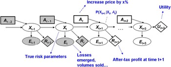
Figure 9 provides the generic structure for a DDN, and its interpretation for our R-Age example. The network has been projected for three future periods to visualise the way in which a network like this is “solved”: since the problem of finding the optimal strategy is intractable, the way one produces a (sub-optimal) strategy is by a look-ahead method:

Figure 9

An insurance company pricing decision process seen as a dynamic decision network.

1. 1. Assume we are at time t

2. 2. Set

3. 3. Explore all possible actions at time

4. 4. For a given action, the updated belief state (not the actual state!) is uniquely determined by the monitoring algorithm explained above

5. 5. Explore all possible “environment actions”, i.e. observations

6. 6. Calculate reward

7. 7. Set and go back to Step 2, until desired look-ahead depth is achieved

8. 8. When desired look-ahead depth is achieved, calculate the utility function in approximate form.

Note that we are using an approximate utility in the method above: if we knew the exact utility, we would not need a look-ahead algorithm – we could directly calculate U_t! Also note that looking ahead only a few steps is usually sufficient when the discount factor used is small enough, as the rewards beyond a certain level might be negligible.

Note that since this exhaustive search is possible only for a discrete number of states, the problem needs to be discretised in a sensible way before carrying out the computation (see Russell & Norvig (2003) for a discussion of computational complexity issues). Also, stochastic search over a random sample of actions and observations can sometimes replace exhaustive search, as in dynamic financial analysis exercises.

Overall, POMDPs and especially dynamic decision networks represent a good way of representing risk agents such as an insurance company, at least in situations that are not too complex. Various approximation methods – beyond those illustrated here – can be used to make near-optimal decisions with reasonable computational complexity. The interested reader is referred as usual to Russell & Norvig (2003) for a more thorough treatment of these techniques (see especially Chapter 21 on reinforcement learning).

The reader will have noticed analogies with ruin theory, dynamic financial analysis and pricing optimisation. As a matter of fact, all these theories/activities can be put in the context of risk agents making decisions in an uncertain environment:

• • POMDPs are an extension of ruin theory in the sense that they also enable us to consider the effect of decisions and other uncertainties (including model and data uncertainty) on the probability of ruin in a Bayesian context;

• • DFA is a special case of POMDPs where utility is calculated for a random sample of possible actions and observations – possibly in an interactive fashion;

• • pricing optimisation can also be put into the context of POMDPs: in this case the demand modelling is given special emphasis.

4.5 Towards more realistic examples

The R-Age example outlined at the beginning of Section 4 was of course simplistic: an insurer trading in a single class of business, charging all customers the same amount, facing no direct competition, and knowing both the parameters of the loss distribution and the demand curve perfectly.

As we have seen in Section 4.3, POMDPs allow us to lift the assumption about knowing the loss distribution perfectly: the parameters of the loss distribution can be learned gradually as time progresses. If the distribution changes with the time, as it probably will, the changing parameters can still be learned if the changes are not too quick (see Section 3). Analogous considerations can be made about the demand curve, which needs to be learned as we go along.

Other assumptions, such as the fact that R-Age deals only with one product and charges all customers the same amount, have allowed us to simplify the problem but have not changed its nature, and were made only for clarity of treatment. Having multiple products, and different classes of customers, does not change the problem in principle: however, the resulting optimisation problem is far more complex, and the solution might be one in which the pricing of some or all the products is significantly sub-optimal: e.g. cross-subsidisation is a case in point.

A far more crucial assumption, however, was that R-Age was the only player in its niche market. When this is not the case, learning the characteristics of the environment as a whole – which includes not only the loss process and the customers but also the competitors and many other players – becomes an altogether different challenge, which will be addressed in the next section.

5.1 Multi-agent systems (MAS)

Multi-agent systems are collections of intelligent agents, which interact both with the environment and among themselves. They can be used in a cooperative or non-cooperative fashion. For example, agents may cooperate to solve a given problem, by breaking it up into smaller tasks: this is a familiar use of agents in a software engineering context. Alternatively, they can be made to compete with each other. In this latter non-cooperative framework, which is the most interesting to us, there are two main ways in which we can use multi-agent systems:

• ▪ Agent design: designing agents that deal with other agents with an optimal strategy, so as to maximise their utility.

• ▪ Mechanism design: designing rules to regulate the interaction between different agents in order to maximise some overall measure of utility.

If we look at insurance companies as agents, agent design is what is required for an insurance company which wants to thrive among its competitors, or that of an individual wanting to buy a household policy. Mechanism design is instead the job of the regulator. When devising new regulations, it is important to understand what the effect of the regulation is going to be, and to test different types of regulations so as to reduce the instability of the system. This effect can only be understood at the collective, and not at the individual, level.

An example which follows this spirit although it ignores the formalism of multi-agent systems is the paper presented at GIRO 2008 by Taylor (Taylor, Reference Taylor2008), which investigates the effect of catastrophes and of regulation on producing cyclical effects such as the underwriting cycle.

5.2 Games of partial information

Game theory plays a role whenever there are agents that have to adopt successful interaction strategies, and can be used for both agent design and mechanism design. The games we are mostly interested in when modelling the behaviour of the insurance markets:

• ▪ are repeated games, in which agents meet one another repeatedly and keep memory of the previous encounters;

• ▪ involve several different agents making decisions simultaneously;

• ▪ concern information which is only partially observable, in the sense that each agent has only partial information on what its opponents are doing;

• ▪ have stochastic payoffs, at least because of randomness of the loss process;

• ▪ are mostly non-cooperative, as the insurance market is competitive.

Games in this type of setting are called games of partial information. Popular examples include card games such as poker and bridge, in which each player can only see a subset of the cards, or the modelling of nuclear wars, where the location of the opponents’ weapons is unknown. Games of partial information can be solved theoretically by similar techniques to those used in Section 3.4, where a solution maximising utility was outlined by a look-ahead technique. A key difference is that one's belief state is observable whereas that of the opponents are not.

However, game theory has not been widely used for agent design. According to Russell & Norvig (2003), there are two main reasons for this:

• ▪ In a Nash equilibrium solution, a player is assuming that the opponents will play the equilibrium strategy, without being able to incorporate any prior belief that the player might have of what the opponent(s) might do. To address this problem, the notion of Bayes-Nash equilibrium has been introduced which explicitly incorporates our prior beliefs about the other players’ likely strategies.

• ▪ No good way is currently known to combine game theory with POMDP theory in the framework of agent design.

For these reasons, game theory has been more successful in mechanism design, by which one attempts to maximise some global utility, basically attempting to discourage behaviours on the part of individual agents which might decrease the overall utility. This can be obtained by the imposition of rules that incorporate all externalities – that is, effects on global utility not recognised in the interaction between agents – explicitly. This has been successfully used for example in designing auctions (Wooldridge, Reference Wooldridge2001; Russell & Norvig, 2003). Another example, which is more directly related to general insurance, regards the optimal allocation of quotas of risk among insurers that evaluate risk differently (Fragnelli & Marina, Reference Fragnelli and Marina2003; Ambrosino et al., Reference Ambrosino, Fragnelli and Marina2006).

In most cases concerning general insurance, an analytical solution of games involving risk agents will of course be impossible, given the large uncertainties and the large number of variables involved. The most promising application of game theory to multi-agent systems in insurance is perhaps through the stochastic modelling of agents, much along the lines of the work done by Axelrod (Reference Axelrod1984) on the evolution of cooperation. Axelrod devised a tournament among agents (represented as programming code) that would meet repeatedly at random and could choose at each encounter whether to “co-operate” or “defect”. The payoff matrix was devised in such a way that mutual cooperation was preferred to mutual defection, whereas the best outcome for an agent would occur when the agent defected while the opponent cooperated. The idea was to have a repeated version of the famous prisoner's dilemma, in which the most rational decision is for both players to defect. The fact that the game is repeated creates a long-term incentive to cooperate (to avoid retaliation), which makes the game more realistic.

The key ideas of the Axelrod experiment are its stochastic nature (agents meet at random) and that rather than trying to design an optimal agent based on theoretical considerations (which proves to be extremely complicated even in simple settings such as this), one can design “tournaments” to test different strategies, and tentatively adopt the strategy which performs better in a number of tournaments.

5.3 A possible approach to modelling the interaction among risk agents

In the light of the discussions in the previous sections, one possible approach to modelling risk agents is as follows (a more detailed example can be found in Parodi, Reference Parodi2009):

1. (i) Model each agent (e.g. an insurer, a customer, a reinsurer, etc) as a POMDP;

2. (ii) model the interaction between the risk agents as a game of partial information, where the state of one agent depends on the previous actions not only of the agent itself but of the other agents as well, and the risk agents have a (partial) knowledge of the other agents’ strategies;

3. (iii) test the goodness of strategies by stochastic simulation, by having different strategies compete in an Axelrod-style experiment (not necessarily by one-to-one encounters, but by synchronised decisions).

This framework is in principle suitable to address both the agent design and the mechanism design problem. Note, however, that the balance between that information which is publicly available and that which is privately held by the risk agents may vary depending on the context, and especially between the agent design context and the mechanism design context. For example, the regulator might have a more in-depth view of the position of the different risk agents. Obviously, the optimal strategy will vary depending on the amount of information available.

One weakness of this approach is that by testing strategies in this way there is no assurance that optimality is achieved. Actually, the uncertainties involved in the process are so large that there are doubts that the solution is even sub-optimal. One must of course be aware that the level of complexity of even the most basic model is so high that there is a danger that we are able to reproduce well-known phenomena (underwriting cycle, etc) in a spurious fashion, simply because the number of parameters is sufficient to imitate those phenomena by appropriate tuning. At the same time, even the most complicated version of the model will pale in comparison with the messy reality of the insurance market and will not be realistic. Why bother, then? There are at least two reasons to attempt this investigation anyway:

• • Although stochastic simulation of market behaviour will not reproduce the reality of the insurance market in an exhaustive way, it may bring to light unexpected collective phenomena;

• • if we are able to reproduce known phenomena (bubbles, cycles, etc) with a very small number of parameters, and with a broad range of parameter values (that is, robustly), we may indeed have found something which has predictive value and that could be used for further investigation.

The overriding consideration should be to consider these models with much caution, as useful tools for exploratory analysis rather than rigorous means of understanding collective behaviour.

5.4 A practical example from financial modelling

An example which is very much in the spirit of the approach outlined in Section 5.3 can be found in the paper by Darley et al. (Reference Darley, Outkin, Plate and Gao2001) “Learning, evolution and tick size effects in a simulation of the Nasdaq stock market”. As the title suggests, this example comes from the field of financial modelling rather than from that of non-life insurance. However, I believe it is worth including it as it may easily provide a template for an analogous insurance exercise.

The authors provide an agent-based model of the stock market. The model is structured as follows:

1. i. Market makers and investors are modelled as individual agents.

2. ii. The market is made of a single security whose true value (or fundamental value) is assumed to fluctuate as the result of a stochastic process.

3. iii. Investors do not know the true value, but a noisy version of it.

4. iv. Each agent behaves according to its individual strategy, e.g. you have investors who make their decision based on the true value they estimate, and those that act based on estimated trends. Market makers can also make use of information not available to the investors, e.g. all the trades they are involved in.

5. v. The individual strategies are either built in or “learned” based on market data – which allows for the discovery of new strategies.

Agents are then made to compete against one another in the market with a stochastic simulation. Based on this set-up, the authors have obtained a number of interesting results. We cite two of them, the first related to mechanism design and the second to agent design:

• • reducing the tick size (i.e. the minimum amount by which stock prices can change) below a certain limit makes it more difficult for participants to discover the “true” value of the security (price discovery), if parasitic strategies such as day traders are allowed;

• • under a variety of conditions, artificial learning strategies were seen to outperform built-in strategies based on expert knowledge or extracted from data.

As mentioned at the beginning of this section, this work may provide a template for similar works in an insurance context:

• • the “price discovery” problem that Darley et al. (Reference Darley, Outkin, Plate and Gao2001) addresses is not at all dissimilar from the problem of determining the pure cost of an insurance policy;

• • as in the stock market, the market participants (insurers and insureds) never see the “true value” (fundamental value) of the policy, but only a noisy version of it, the noise coming from various sources of uncertainty: process, parameter, model and data uncertainty;

• • whilst the stock market has constraints such as the tick size, the insurance market has its own constraints – such as capital requirements – on market participants. Stochastic simulation will help discover unintended consequences of these constraints;

• • pricing strategies may be tested against one another, exactly as investing strategies in the stock market. Furthermore, it will be possible to compare “expert” strategies which attempt to replicate the behaviour of actual players in the market with artificial learning strategies.