


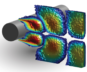

1. Introduction
Flow over a circular cylinder has received a great deal of research interest for decades due to its prevalent occurrence in various real-world engineering applications. Different types of circular cylinder configurations from single to tandem are found in many transportation systems such as aircraft landing gears (Lockard & Lilley Reference Lockard and Lilley2004) and high-speed train pantographs (Sueki, Ikeda & Takaishi Reference Sueki, Ikeda and Takaishi2009). Electrical power lines (Blevins Reference Blevins1984), chimney stacks (Zdravkovich Reference Zdravkovich1981) and offshore wind turbine towers (Youssef et al. Reference Youssef, el Moctar, el Sheshtawy, Tödter and Schellin2022) are other practical examples of circular cylinders. Vortex shedding is a well-established phenomenon in these applications that may lead to acoustic noise (Strouhal Reference Strouhal1878; von Kármán Reference von Kármán1912; Curle Reference Curle1955), structural vibrations (Bearman & Branković Reference Bearman and Branković2004; Sarpkaya Reference Sarpkaya2004; Williamson & Govardhan Reference Williamson and Govardhan2004) and unsteady lift and mean drag forces (Etkin, Korbacher & Keefe Reference Etkin, Korbacher and Keefe1956; Keefe Reference Keefe1962). The application of active flow control techniques to alleviate the vortex shedding of circular cylinders has grown significantly in the last years (Choi, Jeon & Kim Reference Choi, Jeon and Kim2008). Implementing active flow control methods typically involves integrating actuators, sensors and control systems, which can add complexity and cost to the overall system. Moreover, these techniques often require a power source to operate the actuators and control the flow patterns. Despite these challenges, active flow control offers the advantage of controllability, enabling manipulation of dynamic and complex processes during system operation. This flexibility allows for dynamic optimisation and adaptation to changing flow conditions, ensuring optimal performance and efficiency across various operating scenarios. Active flow control can be tailored to target specific flow features or phenomena, such as vortex shedding from circular cylinders, by adjusting the control parameters to influence the vortex location, strength or shedding frequency. Many types of cylinder active flow control techniques such as synthetic jets, electromagnetic forcing, rotation, forced oscillation, thermal effects, acoustic excitation, moving surfaces, feedback control strategies and suction/blowing (the latter is the focus of this study) were investigated at length as reviewed by Rashidi, Hayatdavoodi & Esfahani (Reference Rashidi, Hayatdavoodi and Esfahani2016) and Chen et al. (Reference Chen, Huang, Chen, Yu and Gao2022).
Among the many possibilities for controlling the primary characteristics of vortex structures, fluid injection from the base of the cylinder (applied at a position  $180^{\circ }$ from the front stagnation point) has attracted attention over the years. This technique is usually identified with flow–structure interaction and was investigated through the pioneering experimental work of Wong (Reference Wong1985) who demonstrated the effectiveness of the base blowing concept in attenuating fluid-induced oscillation when blowing is applied through slits extending along the span of the cylinder. The experiments covered a range of Reynolds numbers (
 $Re=U_{\infty }D/v$), spanning from 2000 to 3000, where
 $U_{\infty }$ (
 ${\rm m}\ {\rm s}^{-1}$) is the free stream velocity,
 $D$ (m) is the cylinder diameter and
 $v$ (
 $\mathrm {N}\ \mathrm {m}^{-3}$) is the kinematic viscosity of the fluid. This research highlighted the potential of base blowing as an efficient method for vortex control. At low Reynolds numbers ranging from
 $10$ to
 $90$, Delaunay & Kaiktsis (Reference Delaunay and Kaiktsis2001) conducted an investigation into the impact of base blowing on the stability and dynamics of the flow around a circular cylinder using numerical simulation and global stability analysis. Their findings indicated that while slight blowing did not affect the shedding frequency, it was effective in stabilising the wake by reducing backflow and, consequently, decreasing absolute instability in the near-wake region. After a considerable lapse in this research domain, Gao et al. (Reference Gao, Chen, Chen, Huang and Li2019) conducted an experimental study to investigate the impact of base jets, emitted from four nozzles into the wake of a circular cylinder, on vortex shedding at
 $Re=3.33\times 10^{4}$. The experimental results demonstrated that distributing base jets along the span length of
 $3D$ altered the vortex-formation pattern and reduced both the drag and lift coefficients by introducing perturbations into the unsteady and asymmetric flows in the cylinder wake. Compared with the baseline configuration, the recirculation regions behind the controlled cylinder were observed to elongate and shift downstream. Building upon a similar concept, Deng et al. (Reference Deng, Gao, Chen and Chen2021) employed a slot jet with a span length of
 $D$ at the base of the cylinder to manipulate vortex shedding at
 $Re=2.17\times 10^{4}$. Their study revealed that a pair of symmetric jet vortices, generated by the slot, played a primary role in modifying the flow structures in the cylinder wake. The dynamic interaction between these vortices and the shear layers led to the elongation of the unsteady separation flows originating from the upper and lower surfaces of the cylinder. As a consequence, the alternating vortex shedding was propelled downstream.
Although this literature review shows well the role of base blowing in manipulating vortices or reducing the drag and lift forces, it does not fully address the effectiveness of this technique in completely suppressing the global instabilities of the wake region. The flow behind a circular cylinder exhibits two types of local instability: near-wake velocity profiles are typically absolutely unstable, while intermediate wake profiles are convectively unstable (Delaunay & Kaiktsis Reference Delaunay and Kaiktsis2001). As a result, the vortex-shedding process can be considered as a saturated nonlinear state of global instability triggered by the absolutely unstable region. To induce self-sustained oscillations, a sufficiently large region of absolute instability is required (Williams, Mansy & Amato Reference Williams, Mansy and Amato1992). It has been reviewed well by Norberg (Reference Norberg2003) that the spanwise correlation length of the cylinder varies between  $9.5D$ and
 $D$ for the Reynolds number ranging approximately from
 $Re=250$ to
 $10^{5}$. This is clear evidence that the three-dimensionality of the flow along the cylinder span is not reduced by only injecting air either through a short slot/slit or only a few nozzles. Thus, there is an obvious gap in the existing literature and further research is required.
The noise generated by the flow over a circular cylinder is primarily attributed to vortex shedding, making the suppression of vortex shedding a crucial aeroacoustic challenge. This issue has been of interest since the 1870s, when the first pioneering studies were conducted to understand the mechanism leading to the vortex-induced noise of a circular cylinder (Strouhal Reference Strouhal1878; von Kármán Reference von Kármán1912; Curle Reference Curle1955). The resulting noise is tonal and is generated as a result of the hydrodynamic pressure field associated with the rolling up of vortex streets from both sides of the cylinder. (von Kármán Reference von Kármán1912; Curle Reference Curle1955; Norberg Reference Norberg1986). Extensive research has been conducted in the past using experiments and simulations (Casalino & Jacob Reference Casalino and Jacob2003; Jenkins et al. Reference Jenkins, Khorrami, Choudhari and McGinley2005; Khorrami et al. Reference Khorrami, Choudhari, Lockard, Jenkins and McGinley2007; Oguma, Yamagata & Fujisawa Reference Oguma, Yamagata and Fujisawa2013; Maryami et al. Reference Maryami, Arcondoulis, Liu and Liu2023c; Maryami, Arcondoulis & Liu Reference Maryami, Arcondoulis and Liu2024b; Maryami et al. Reference Maryami, Arcondoulis, Guo and Liu2024a) to understand and address the specific characteristics of tonal noise generated by cylinders placed individually or in close proximity to one another. Given the effectiveness of base blowing in suppressing vortex shedding by stabilising the near-wake region, it is reasonable to expect that this technique serves as a noise control method in addition to being a flow control method. As such, base blowing offers promising potential for reducing the tonal noise produced by a circular cylinder. The distributed blowing through the surface of a cylinder has been shown to reduce interaction noise resulting from an unsteady wake impinging on a downstream body. Angland, Zhang & Goodyer (Reference Angland, Zhang and Goodyer2012) demonstrated when a cylinder was upstream of an H-beam, blowing resulted in a noise reduction of 9.2 dB at a Strouhal number ( $St=f\kern 0.06em D/U_{\infty }$, where
 $f$ (Hz) is the frequency) of
 $St\approx 0.2$ and this reduction increased to approximately 15 dB at
 $St\approx 0.8$ when the configuration was reversed, with the H-beam upstream of the cylinder. More recently, a comprehensive experimental study conducted by Maryami et al. (Reference Maryami, Arcondoulis and Liu2024b) explored the performance of local blowing (LB) applied around the cylinder symmetrically at angles corresponding to the boundary layer, shear layers on the cylinder and separated shear layers, i.e.
 $\theta =\pm 41^{\circ }$,
 ${\pm }90^{\circ }$ and
 ${\pm }131^{\circ }$, respectively, with a focus on noise reduction. By simultaneously analysing near-field pressure, far-field noise and the flow field, the study revealed the significant potential of LB at
 $\theta ={\pm }41^{\circ }$ in altering the downstream behaviour of vortex shedding and effectively mitigating far-field noise. Expanding on this groundwork, Maryami et al. (Reference Maryami, Arcondoulis, Guo and Liu2024a) conducted a parametric study exploring the noise reduction capabilities of base blowing and illustrated that this technique exhibits performance comparable to LB at
 $\theta =\pm 41^{\circ }$ in terms of tonal noise reduction and even surpasses it in terms of overall sound pressure level (OASPL). Despite these promising results, there is surprisingly limited research on the acoustic effects of base blowing. One possible reason for the lack of experimental studies may be the challenge of acoustic measurement in the far field. The introduction of blowing inevitably adds additional noise, which can decrease the signal-to-noise ratio of the far-field acoustic measurements (Angland et al. Reference Angland, Zhang and Goodyer2012; Guo et al. Reference Guo, Maryami, Yang, Yang, Wang and Liu2023). As a result, conducting accurate acoustic measurements in the presence of blowing can be challenging compared with other flow control techniques. Nonetheless, understanding the acoustic performance of base blowing is essential for further exploring its potential as a noise control method, particularly in the context of vortex shedding and its associated tonal noise.
In their study, Inoue & Hatakeyama (Reference Inoue and Hatakeyama2002) observed that sound waves primarily originate from vortex shedding of the cylinder surface into the wake. Later, Oguma et al. (Reference Oguma, Yamagata and Fujisawa2013) investigated cylinder near-field sound sources using a cross-correlation coefficient analysis between pressure fluctuations in the near field and measured sound pressure fluctuations in the far field. By reconstructing the near-field pressure from the velocity field obtained via particle image velocimetry (PIV), they identified the pressure fluctuation around the flow-separation point on the cylinder surface as a sound source. Additionally, in the near-wake of the circular cylinder, the oscillating flow just behind the cylinder was found to be another sound source. These findings align with the observations of Tamura & Tsutahara (Reference Tamura and Tsutahara2010), who performed direct numerical simulations and proposed that the oscillating flow just behind the cylinder serves as a sound source for low Mach number flows. These studies highlight the importance of understanding the correlation between near-field pressure, far-field noise and the hydrodynamic velocity field in the wake (herein referred to as oscillating wake) to comprehend the noise generation mechanism of a circular cylinder. Despite the valuable insights gained from these studies, there remains a gap in the literature concerning experimental investigations, particularly in the case of base blowing. Experimental studies providing such detailed information are still lacking, emphasising the need for further research in this area.
In addressing the earlier outlined gaps regarding energy consumption in active flow control methods, determining sufficient span length for base blowing, exploring the noise reduction potential of base blowing and achieving simultaneous measurement of multiple fields, the present experimental study deliberately maintained low input energy of base blowing to ensure efficient operation. Furthermore, the base blowing was implemented across an extensive span of the cylinder, covering a distance of  $7D$. To minimise additional noise generated by the blowing process, a relatively quiet air supply system was employed, delivering air to a specially designed chamber. The experimental set-up included a circular cylinder with strategically positioned pressure taps to measure surface pressure fluctuations. Employing a remote-sensing method, pressure measurements were synchronised with far-field noise and velocity field measurements using PIV. To the authors’ knowledge, no similar experimental study has investigated cylinder wake flows, either with or without base blowing, while simultaneously providing three field measurements. This comprehensive approach is expected to illuminate the understanding of flow and noise characteristics influenced by vortex shedding and base blowing, thereby filling crucial gaps in the existing literature.
The remainder of the paper is organised as follows. The experimental set-up, the cylinder design and the methodology of the remote-sensing and PIV are described in § 2. The results and discussions are detailed in § 3. Finally, § 4 concludes the paper and summarises our findings on the application of base blowing for flow and noise control of a circular cylinder.
2. Methodology
Experimental campaigns including near- and far-field measurements and PIV tests were conducted in a low-speed, open-jet anechoic wind tunnel at the Southern University of Science and Technology (SUSTech) (Yang et al. Reference Yang, Liu, Liu, Shen, Zhang, Wei, Liu and Xu2021), as shown in figure 1.
The experimental set-up, depicted in a schematic diagram, showcases a cylinder placed within an aeroacoustic wind tunnel, along with a planar PIV configuration. The coordinate system defines  $x$,
 $y$ and
 $z$ as the directions along the streamwise, vertical (perpendicular to the flow) and spanwise axes, respectively.

2.1. Circular cylinder
The circular cylinder utilised in this study is identical in design to the original cylinder investigated by Maryami et al. (Reference Maryami, Arcondoulis and Liu2024a,Reference Maryami, Arcondoulis, Guo and Liub). The cylinder was constructed in three distinct parts along its span, comprising a middle section with pressure taps and instrumentation for air blowing, as well as two side extension parts, as depicted in figure 2(a). The cylinder possessed an outer diameter of  $D=64.7\ {\rm mm}$ and a span length of
 $L=550\ {\rm mm}$, resulting in a blockage ratio of less than 12 %. With an aspect ratio of approximately 8.5, the cylinder design ensured that any potential influence of the endplates could be disregarded (Zdravkovich Reference Zdravkovich1981).
(a) Schematic diagram of the cylinder design and (b) zoomed-in view of the chamber and sensing area with pressure taps,  ${P}_{i}$ (
 $i=1:20$), distributed around the circumference of the cylinder at midspan. Note that only pressure taps
 ${P}_{5}$ to
 ${P}_{14}$ are visible in this diagram. The peripheral locations of all 20 pressure taps are listed in table 2.

The middle section of the cylinder was covered with a solid layer having inner and outer diameters of  $d=40\ {\rm mm}$ and
 $D=64.7\ {\rm mm}$, respectively, to facilitate air injection over a span length of
 $7D=453\ {\rm mm}$. Previous experimental data available in the literature indicate that the maximum spanwise coherence length of a circular cylinder typically lies within the range of
 $3.3D$–
 $3D$ for Reynolds numbers ranging from
 $Re=0.7\times 10^{5}$ to
 $1.04\times 10^{5}$ (which is the focus of this study) (Norberg Reference Norberg2003). However, there is a lack of precise experimental or numerical data to determine this length for the specific case of LB at a particular Reynolds number and airflow rate. Therefore, a span length of
 $7D$ was chosen to allow for the development of a three-dimensional (3-D) flow field along the span of the cylinder. The solid layer incorporated holes with a diameter of
 $d_{0}=1.2\ {\rm mm}$ to enable distributed blowing through the surface of the cylinder at the peripheral angle of
 $180^{\circ }$, as illustrated in figure 2(b). This blowing technique, referred to as LB180, was implemented through 64 holes with a spanwise spacing of
 $L_{0}=7\ {\rm mm}$. The choice of this spanwise distance between neighbouring holes was made after carefully considering the need for achieving uniform blowing along the span of the cylinder, while also taking into account the practical constraints of the manufacturing process for the solid layer and the air flow chamber through the 3-D printing process.
In this study, the incoming flow velocity was set at  $U_{\infty }=20$ and
 $30\ {\rm m}\ {\rm s}^{-1}$, corresponding to
 $Re=0.7\times 10^{5}$ and
 $1.04\times 10^{5}$, respectively. By considering the Strouhal number relationship (refer to § 1) and
 $St\approx 0.19$ for the anticipated Reynolds number range of a circular cylinder (Norberg Reference Norberg2003), the vortex-shedding frequency is approximately 58 and 86 Hz for
 $U_{\infty }=20$ and
 $30\ {\rm m}\ {\rm s}^{-1}$, respectively. In the same wind tunnel at SUSTech, it was demonstrated by Maryami et al. (Reference Maryami, Arcondoulis, Liu and Liu2023c) that the vortex-shedding tone of a circular cylinder occurs within
 $f\approx 44\unicode{x2013}134\ {\rm Hz}$ for a flow speed range of
 $U_{\infty }=15\unicode{x2013}50\ {\rm m}\ {\rm s}^{-1}$ and typically protrudes above the background noise by at least 10 dB. Therefore, the incoming flow velocities of
 $U_{\infty }=20$ and
 $30\ {\rm m}\ {\rm s}^{-1}$ are sufficient to reach a balance between low background noise and high vortex-shedding frequency. In addition, the Reynolds number range considered here is also matched to the subcritical regime (Roshko Reference Roshko1955; Achenbach Reference Achenbach1968), which is the working flow conditions of typical aeroacoustic applications. For the PIV measurements, however, all tests were carried out at
 $U_{\infty }=20\ {\rm m}\ {\rm s}^{-1}$ to achieve an optimal particle seeding density, an accurate and reliable tracking of the particles within the fluid and hence robust data of flow velocity (Maryami et al. Reference Maryami, Arcondoulis and Liu2024b).
2.2. Airflow chamber
A 3-D printed chamber was embedded firmly under the solid layer and the blowing holes of the chamber were properly aligned with the holes of the solid layer, shown in figure 2(b). More details of the chamber design were presented by Maryami et al. (Reference Maryami, Arcondoulis, Yang, Szoke, Xiang, Guo, Wei and Liu2022b); Maryami, Arcondoulis & Liu (Reference Maryami, Arcondoulis and Liu2023a,Reference Maryami, Arcondoulis and Liub); Maryami et al. (Reference Maryami, Arcondoulis and Liu2024a,Reference Maryami, Arcondoulis, Guo and Liub). The chamber was divided at the half-span of the cylinder for two advantages. First, it allowed embedding the remote-sensing pressure ports at the midspan without interrupting the air flow inside the chamber. Second, it was possible to supply airflow from both ends of the chamber, where each side was fed by eight inlets for tube connections (see figure 2a), resulting in a more uniform blowing along the chamber span. The static pressure was measured to check the uniform blowing only along the half-span length of the chamber due to symmetry. The 32 steel tubes with inner and outer diameters of 0.5 and 1 mm, respectively, were inserted into the chamber holes and were connected to pressure scanners by flexible tubes with an inner diameter of 0.5 mm and an outer diameter of 2 mm. Two 16-channel Model 9116 intelligent pressure scanners with a full-scale pressure range from 2.5 kPa to 5200 kPa were used to perform the static pressure measurements. The pressure scanners are capable of accuracies up to  ${\pm }0.05\,\%$. The results showed that the pressure along the chamber span is constant within
 ${\pm }1\,\%$ (Maryami et al. Reference Maryami, Arcondoulis and Liu2024b).
The blowing rate was measured by a temperature-compensated flow meter and was kept constant by a regulator and pressure gauge. For each Reynolds number, the experiments were carried out for three air flow rates of  $Q_{b}\approx 8.5$, 14 and 20
 ${\rm m}^{3}\ {\rm h}^{-1}$. The equivalent momentum coefficient,
 $C_{\mu }$, was used to facilitate the research (Maryami et al. Reference Maryami, Arcondoulis and Liu2024a,Reference Maryami, Arcondoulis, Guo and Liub). This coefficient is the ratio of blowing momentum flux at each hole to incoming flow momentum flux and is calculated via
 \begin{equation} C_{\mu}=\left(\frac{U_{b}}{U_{\infty}}\right)^{2}\times\left(\frac{A_{b}}{DL_{0}}\right)\!, \end{equation}
where  $U_{b}$ (
 ${\rm m}\ {\rm s}^{-1}$) is the average blowing velocity of each hole,
 $A_{b}$ (
 $\mathrm {m}^{2}$) is the area of each hole and
 $L_{0}$ (m) is the spanwise spacing between two neighbouring holes. The values of
 $C_{\mu }$ and the associated properties of blowing are presented in table 1.
Blowing flow rate,  $Q_{b}$ (
 ${{\rm m}^{3}\ {\rm h}^{-1}}$), blowing flow velocity,
 $U_{b}$ (
 ${\rm m}\ {\rm s}^{-1}$) and their corresponding
 $C_{\mu }$ values calculated using (2.1).

2.3. Steady and unsteady surface pressure measurements
In this study, the circular cylinder was equipped with 20 pressure taps strategically distributed around its circumference with non-uniform angular spacing, as illustrated in figure 2(b). Each pressure tap was labelled and its corresponding angular distance from the front stagnation point ( $\theta =0^{\circ }$) was presented in table 2. These pressure taps were designed as brass tubes with inner and outer diameters of 0.8 mm and 1.6 mm, respectively, passing through the housing in the solid layer and flush with its outer diameter. Steady pressure measurements were obtained by connecting the brass tubes to the intelligent pressure scanners through polyurethane tubes with inner and outer diameters of 0.8 and 4 mm, respectively, following the approach detailed in previous work by Maryami et al. (Reference Maryami, Arcondoulis, Liu and Liu2023c,Reference Maryami, Arcondoulis, Yang and Liud). To ensure a smooth pressure distribution, the baseline was rotated three times by an angle of approximately
 $8^{\circ }$, allowing data to be collected at 45 unique peripheral angles. However, for LB180, rotating the cylinder was not possible, and hence, the results were provided only at 20 angular locations.
Peripheral positions of pressure taps,  ${P}_{i}$ (
 $i=1:20$), at
 $z/D=0$.

The unsteady pressure, which represents surface pressure fluctuations, was measured using a remote-sensing technique through the same pressure taps utilised for steady pressure measurements. The pressure taps were connected to remote-sensing probes using brass and flexible polyurethane tubing, acting as wave guides, as depicted in figure 3(a). It is important to note that pressure fluctuations on the surface of the cylinder can propagate as acoustic waves through the tubes. The remote-sensing probe consisted of a microphone holder, an acoustic termination tube and a Panasonic WM-61A microphone attached to a pinhole with a diameter of 0.4 mm. To prevent sound wave reflections caused by viscous dissipation and the generation of spurious tones related to standing waves in the flexible tubing, a 2-m-long termination tube was placed after the microphone. This set-up ensured accurate and reliable measurements. The Panasonic WM-61A microphone is known for its flat frequency response, covering the range from 20 Hz to 10 kHz, as specified by the manufacturer and widely acknowledged in previous studies (Angland et al. Reference Angland, Zhang and Goodyer2012; Maryami et al. Reference Maryami, Azarpeyvand, Dehghan and Afshari2019, Reference Maryami, Showkat Ali, Azarpeyvand and Afshari2020; Vemuri et al. Reference Vemuri, Liu, Zang and Azarpeyvand2020; Maryami et al. Reference Maryami, Ali, Azarpeyvand, Dehghan and Afshari2022a, Reference Maryami, Arcondoulis, Liu and Liu2023c, Reference Maryami, Arcondoulis and Liu2024a,Reference Maryami, Arcondoulis, Guo and Liub).
Schematic of the remote-sensing set-up. (a) Full view of the cylinder with calibration set-up and (b) assembly view of the remote microphone probe.

In-situ calibration was performed to account for any potential amplitude damping within the small tubes and the lag caused by the extensions of the remote probe. For this purpose, an in-house-designed calibrator (see figure 3a) was utilised, comprising a high-quality loudspeaker connected to a 3-D printed cone filled with porous material and a tube with a length of 110 mm and a diameter of 10 mm. This calibration set-up is similar to that used by Maryami et al. (Reference Maryami, Azarpeyvand, Dehghan and Afshari2019). To conduct the calibration, a 1/2-in. Brüel and Kjær free-field microphone Type 4966 was placed close to the pressure tap, serving as the reference microphone. A planar white noise signal was generated by the loudspeaker to calculate the transfer function, denoted as  $T_{RM}$, between the remote-sensing probe and the reference microphone via
 \begin{equation} T_{RM}(\,f)=\frac{\phi_{MM}(\,f)}{\phi_{RM}(\,f)}, \end{equation}
where  $\phi_{MM}\ ({{\rm Pa}^{2}\,{\rm Hz}^{-1}})$ is the autospectrum of the remote-sensing signals and
 $\phi_{RM}\ ({{\rm Pa}^{2}\ {\rm Hz}^{-1}})$ is the cross-spectrum between the reference and remote-sensing signals. Note that both the reference and remote-sensing pressure measurements were conducted simultaneously. The coherence values between these pressure signals were found to be smooth and near unity for frequencies up to approximately 6 kHz, which aligns with similar frequency ranges observed in other studies (Garcia-Sagrado & Hynes Reference Garcia-Sagrado and Hynes2011; Gruber Reference Gruber2012). The upper limit of this frequency range corresponds to
 $St\approx 13$ at
 $U_{\infty }=30\ {\rm m}\ {\rm s}^{-1}$, which is sufficiently high for covering the relevant frequency range in this experimental study.
The far-field noise measurements were conducted using a Brüel and Kjær free-field Type 4966 microphone positioned at an angle of  $90^{\circ }$ to the flow and a distance of 1.5 m away from the cylinder axis, as illustrated in figure 1. Both near- and far-field noise measurements were obtained simultaneously with a sampling frequency of 51.2 kHz for a duration of 10 s, employing two 24-bit synchronised National Instruments (NI) PXI-4496 data acquisition (DAQ) cards installed in an NI PXI-10420 chassis. To convert the acquired pressure–time data into the frequency domain, a fast Fourier transformation with Hamming windowing and 50 % overlap, using Welch's method, was employed, resulting in a frequency resolution of 2 Hz. These data were subsequently transformed into power spectral density (PSD), denoted as
 $\phi _{pp,s}$ and
 $\phi _{pp}$ (
 ${{\rm Pa}^{2}\ {\rm Hz}^{-1}}$) for the near- and far-field pressures, respectively. The PSD values were referenced to a baseline pressure of
 $p_{_0}=20\,\mathrm {\mu }{\rm Pa}$ as follows:
 \begin{equation} \varPhi_{pp}=10\log_{10}\left(\frac{\phi_{pp}}{p^{2}_{0}}\right)\!. \end{equation}
To assess the precision of  $\phi _{pp,s}$ and
 $\phi _{pp}$ spectra, it is essential to account for factors such as frequency sampling, recording time, sub-blocks, window size and overlap. Following the convergence error estimation methods for Fourier transform (Bendat & Piersol Reference Bendat and Piersol2011), this study focused on analysing random errors. Utilising 26 sub-blocks results in an error of approximately 0.76 dB for both
 $\phi _{pp,s}$ and
 $\phi _{pp}$, calculated by
 $10\log _{10}(1+1/\sqrt {N_{b}})$, where
 $N_{b}$ is the number of sub-blocks (Maryami et al. Reference Maryami, Arcondoulis, Guo and Liu2024a). Moreover, the confidence intervals at a 95 % confidence level for
 $\phi _{pp,s}$ and
 $\phi _{pp}$ at the vortex-shedding frequency were determined as (
 $-$0.85 dB, 0.71 dB) and (
 $-$0.15 dB, 0.16 dB), respectively.
2.4. The PIV experiments
Planar PIV measurements were performed at a high repetition rate for the near-wake region at  $U_{\infty }=20\ {\rm m}\ {\rm s}^{-1}$ and
 $C_{\mu }=0.007$. The field of view (FOV) in the experiment covers the flow field with dimensions of
 $5D\times 3D$ in the
 $x$- and
 $y$-directions, respectively, as depicted in figure 4(a). The flow was seeded with dioctyl sebacate particles with an average diameter of
 $1\,\mathrm {\mu }\mathrm {m}$. A Photonics Nd: YAG laser (50 mJ at 10 kHz) was used to provide illumination. To facilitate particle illumination on both the top and bottom sides of the wake centreline, the light sheet was directed from the wake towards the cylinder as shown in figure 4(b). With a distance of approximately 1500 mm between the cylinder centre and the final lens of the laser, it can be confidently affirmed that the lens has a negligible influence on the flow field around the cylinder. A Phantom VEO410L (
 $1280\times 780$ pixels, 12 bit, pixel pitch
 $20\,\mathrm {\mu }\mathrm {m}$, maximum frame rate 5.2 kHz) equipped with a Nikon Micro-Nikkor 60 mm objective was used at a focal ratio of
 $f/2.8$. Synchronisation of the laser pulses and image acquisition was conducted using a LaVision programmable timing unit in combination with the LaVision DaVis 10.0 software package. All
 $5289$ images were obtained at a frequency of 2.645 kHz for 2 s, which is sufficiently higher than the expected vortex-shedding frequency of the cylinder at
 $U_{\infty }=20\ {\rm m}\ {\rm s}^{-1}$ (i.e.
 $f=58$ Hz). Image correlation was carried out with an iterative multipass technique with a final window size of 32
 $\times$32 pixels and an overlap factor of 75 %.
Schematic diagram of planar PIV configuration: (a) top view and (b) side view.

Considering the camera's technical specifications and the interrogation window, the spatial resolution is approximately  $(20\,\mathrm {\mu }\mathrm {m}\times 1280)/32\approx 0.8\ {\rm mm}\,{\rm pixel}^{-1}$ in the horizontal direction and
 $(20\,\mathrm {\mu }\mathrm {m}\times 780)/32\approx 0.5\ {\rm mm}\,{\rm pixel}^{-1}$ in the vertical direction. The turbulence intensity of the flow at the cylinder's streamwise location is represented by
 $\sigma _{u}=15\,\%$. The uncertainty in the mean velocity field is calculated using
 $\epsilon _{u}={\sigma _{u}}/{\sqrt {N_{p}}}\approx 0.2\,\%$, where
 $N_{p}$ corresponds to the number of PIV temporal samples. Similarly, the uncertainty in the streamwise velocity fluctuations is determined as
 $\epsilon _{u'}={\sigma _u}/{\sqrt {2(N_{p}-1)}}\approx 0.15\,\%$.
To synchronise PIV with the microphone signals, the transistor–transistor logic signal from the Q-switch of the first laser was recorded simultaneously with the microphone signals as proposed by Maryami et al. (Reference Maryami, Arcondoulis and Liu2024b). The signals were acquired using NI PXI-4496 (the same DAQ card as the microphone signal) and sampled with a rate of 51.2 kHz. The NI PXI-4496 DAQ was also triggered by the programmable timing unit to ensure synchronous measurements. As the PIV and pressure signals have different lengths and sampling rates, the signals were resampled at a lower sampling rate using an antialiasing (low-pass) finite impulse response filter. The signals were also aligned by the earliest signal to compensate for any delay.
3. Results and discussion
3.1. Far-field noise spectra
Figure 5(a,b) show the far-field acoustic PSD,  $\varPhi _{pp}$ (
 ${{\rm dB}\ {\rm Hz}^{-1}}$), of each cylinder as a function of
 $St$ for
 $Re=0.7\times 10^{5}$ and
 $1.04\times 10^{5}$, respectively. By inspecting figure 5, it is evident that the baseline reveals the fundamental vortex-shedding tone of a circular cylinder (
 $\varPhi _{pp}\approx 70\ {\rm dB}$), as its corresponding Strouhal number (
 $St\approx 0.19$) lies within the published Strouhal number envelope for these Reynolds numbers (Norberg Reference Norberg2003). This tone is herein referred to as the
 $f_{1}$-tone or the first harmonic. The baseline at
 $Re=0.7\times 10^{5}$ also possess the second and third tones (herein called as the
 $f_{2}$- and
 $f_{3}$-tones, respectively) with even magnitudes of approximately 40 dB, at
 $St\approx 0.38$ and 0.58, respectively. Hence, the
 $f_{2}$- and
 $f_{3}$-tone frequencies are positive integer multiples of the
 $f_{1}$-tone frequency and are known as higher harmonics (i.e.
 $f_{2}=2f_{1}$ and
 $f_{3}=3f_{1}$). The analysis of noise spectral level reveals that the
 $f_{1}$-tone exhibits strong dominance over the
 $f_{2}$-tone, which is consistent with previous studies (Inoue & Hatakeyama Reference Inoue and Hatakeyama2002; Khalighi et al. Reference Khalighi, Mani, Ham and Moin2010; Maryami et al. Reference Maryami, Arcondoulis, Liu and Liu2023c). Research conducted by Gerrard (Reference Gerrard1955) and Etkin, Korbacher & Keefe (Reference Etkin, Korbacher and Keefe1957) has demonstrated that sound wave patterns in the far field exhibit a dipole nature, which is characterised by a dominant fundamental frequency accompanied by multiple harmonics. Specifically, the fundamental tone of the sound radiates most prominently in the direction perpendicular to the free stream, while the second harmonic radiates most strongly in the free stream direction. These observations highlight the characteristics of sound wave patterns in terms of their dominant frequencies and directional radiation in the far field.
Acoustic PSD,  $\varPhi _{pp}$ (
 ${{\rm dB}\ {\rm Hz}^{-1}}$), plotted against
 $St$ at (a)
 $Re=0.7\times 10^{5}$ and (b)
 $Re=1.04\times 10^{5}$. The labels
 $f_{1}$,
 $f_{2}$ and
 $f_{3}$ represent the fundamental vortex-shedding tone (first harmonic), second and third harmonics, respectively.

The LB180 demonstrates the ability to reduce the  $f_{1}$-tone magnitude from that of the baseline, and it is more pronounced by a value of approximately 25 dB when
 $C_{\mu }$ increases to 0.036 at
 $Re=0.7\times 10^{5}$. This can be attributed to the vortex-shedding behaviour which occurs farther downstream in comparison with the baseline as will be further discussed in § 3.4. At
 $Re=1.04\times 10^{5}$, while LB180 exhibits a tonal noise reduction, all
 $C_{\mu }$ values possess a strong tone with very similar magnitudes within 2 dB. The weakest
 $f_{1}$-tone is observed for
 $C_{\mu }=0.016$, with a magnitude of approximately 64 dB. At a Reynolds number of
 $Re=0.7\times 10^{5}$, a reduction in broadband noise is observed in the range of
 $St\approx 0.2$ to 2 for the LB180 technique, and this reduction remains consistent across different values of
 $C_{\mu }$. However, at a higher Reynolds number of
 $Re=1.04\times 10^{5}$, and for all values of
 $C_{\mu }$, LB180 exhibits a broadband spectrum with energy content similar to that of the baseline case. At higher Strouhal numbers, centred at
 $St\approx 8$, a significant contribution of broadband noise is observed particularly at
 $Re=0.7\times 10^{5}$. The observed broadband noise, which intensifies with increasing
 $C_{\mu }$, is solely influenced by the blowing process and is referred to as blowing self-noise. The major blowing self-noise is primarily generated by the compressor, chamber and blowing jets (Angland et al. Reference Angland, Zhang and Goodyer2012; Guo et al. Reference Guo, Maryami, Yang, Yang, Wang and Liu2023; Maryami et al. Reference Maryami, Arcondoulis and Liu2024a,Reference Maryami, Arcondoulis, Guo and Liub). Although not shown here for brevity, it is noteworthy that the ratio of vortex-shedding noise to blowing self-noise is significantly high at
 $C_{\mu }=0.036$. This was also corroborated by Guo et al. (Reference Guo, Maryami, Yang, Yang, Wang and Liu2023) in their research, utilising the identical air supply system at SUSTech and comparable airflow rates. This observation is crucial for assessing the effectiveness of LB180 in mitigating vortex-shedding noise from a circular cylinder.
The OASPL of LB180 relative to the baseline, i.e.  $\Delta {\rm OASPL}$ (dB), is calculated by integrating the far-field PSD over the whole frequency range of interest corresponding to
 $St\approx 0.13\unicode{x2013}13$ as follows:
 \begin{equation} \Delta\mathrm{OASPL}=10\,\log_{10}\left(\frac{\displaystyle\int\phi_{pp}|_{{LB180}}\,\mathrm{d}f} {\displaystyle\int\phi_{pp}|_{{Baseline}}\,\mathrm{d}f}\right). \end{equation}
Table 3 reveals that the OASPL in the case of LB180 is lower than that of the baseline, indicated by  $\Delta \mathrm {OASPL}<0$, particularly at
 $Re=0.7\times 10^{5}$. This finding emphasises the significant contribution of tonal noise to the OASPL for bluff bodies, surpassing the influence of broadband spectral content and blowing self-noise. The noise reduction performance of LB180 becomes more prominent with increasing
 $C_{\mu }$ for both Reynolds numbers. However, there is an exception at
 $Re=0.7\times 10^{5}$, where the noise reduction decreases by 0.07 dB when
 $C_{\mu }$ varies from 0.018 to 0.036. In terms of the variation of
 $\Delta \mathrm {OASPL}$ with respect to Reynolds number, it is observed that at
 $Re=0.7\times 10^{5}$, the maximum value of
 $C_{\mu }$ leads to
 $\Delta \mathrm {OASPL}=-14.88$ dB, while at
 $Re=1.04\times 10^{5}$, it results in
 $\Delta \mathrm {OASPL}=-6.21$ dB.
The  $\Delta \mathrm {OASPL}$ (dB) calculated using (3.1) over the frequency range corresponding to
 $St\approx 0.13\unicode{x2013}13$.

3.2. Near-field pressure spectra
To gain a deeper understanding of the noise reduction mechanism of LB180, the near-field pressure PSD,  $\varPhi _{pp,s}$ (
 ${{\rm dB}\ {\rm Hz}^{-1}}$), is depicted in figure 6 for
 $Re=0.7\times 10^{5}$. As twenty data points were processed for each
 $C_{\mu }$ value, the results are selectively presented at specific peripheral angles, namely
 $\theta =0^{\circ }$,
 $41^{\circ }$,
 $90^{\circ }$,
 $131^{\circ }$ and
 $180^{\circ }$. The spectral analysis of the baseline at all angles, except
 $\theta =180^{\circ }$, reveals a prominent tonal peak corresponding to the
 $f_{1}$-tone frequency, which is consistent with the characteristic vortex-shedding tone observed in figure 5(a). It indicates that vortex shedding is the primary mechanism responsible for the generation of pressure fluctuations on the surface of the cylinder (Norberg Reference Norberg1986; Inoue & Hatakeyama Reference Inoue and Hatakeyama2002; Casalino & Jacob Reference Casalino and Jacob2003; Oguma et al. Reference Oguma, Yamagata and Fujisawa2013; Maryami et al. Reference Maryami, Arcondoulis, Liu and Liu2023c, Reference Maryami, Arcondoulis and Liu2024a,Reference Maryami, Arcondoulis, Guo and Liub). According to Inoue & Hatakeyama (Reference Inoue and Hatakeyama2002), the shedding of a vortex from one side of the cylinder results in a negative pressure pulse on that side, while a positive pressure pulse is induced on the opposite side. These alternating pressure fluctuations on both sides of the cylinder surface serve as sources of sound (Inoue & Hatakeyama Reference Inoue and Hatakeyama2002; Oguma et al. Reference Oguma, Yamagata and Fujisawa2013; Li, Rival & Wu Reference Li, Rival and Wu2021; Maryami et al. Reference Maryami, Arcondoulis, Liu and Liu2023c, Reference Maryami, Arcondoulis and Liu2024a,Reference Maryami, Arcondoulis, Guo and Liub). Further discussion in § 3.4 will elaborate on how these pressure pulses arise from interactions in the shear layer and rapid vertical flow movements within the vortex-formation region. In the baseline case, no peak at the
 $f_{1}$-tone frequency is observed at
 $\theta =180^{\circ }$, and instead, the dominant peak occurs at the
 $f_{2}$-tone frequency. This suggests that these pressure fluctuations have a significant contribution to the fluctuations in drag, which is consistent with findings from previous studies (Casalino & Jacob Reference Casalino and Jacob2003; Maryami et al. Reference Maryami, Showkat Ali, Azarpeyvand and Afshari2020, Reference Maryami, Ali, Azarpeyvand, Dehghan and Afshari2022a, Reference Maryami, Arcondoulis, Liu and Liu2023c, Reference Maryami, Arcondoulis and Liu2024a,Reference Maryami, Arcondoulis, Guo and Liub).
Near-field pressure PSD,  $\varPhi _{pp,s}$ (
 ${{\rm dB}\ {\rm Hz}^{-1}}$), at
 $\theta =0^{\circ }$ (a),
 $41^{\circ }$ (b),
 $90^{\circ }$ (c),
 $131^{\circ }$ (d) and
 $180^{\circ }$ (e) for
 $Re=0.7\times 10^{5}$. The labels
 $f_{1}$ and
 $f_{2}$ represent the fundamental vortex-shedding tone (first harmonic) and second harmonic, respectively.

In figure 6(a), corresponding to  $\theta =0^{\circ }$, LB180 does not exhibit the dominant
 $f_{1}$-tone observed in the baseline. Instead, a significant broadband contribution is observed at
 $St\gtrapprox 4$, which increases in spectral content with
 $C_{\mu }$. Moving away from the stagnation point to
 $\theta =41^{\circ }$,
 $90^{\circ }$ and
 $131^{\circ }$ (see figure 6b–d), the
 $f_{1}$-tone is present in the LB180 spectra for all
 $C_{\mu }$ values, but with a magnitude approximately 20 dB lower than that of the baseline. This can be attributed to the effect of LB180 pushing the vortex-formation region farther downstream, resulting in slower vertical flow movement near the cylinder and weaker near-field pressure at the
 $f_{1}$-tone frequency. At
 $\theta =180^{\circ }$, as shown in figure 6(e), the LB180 spectra exhibit a predominantly broadband behaviour at the
 $f_{1}$-tone frequency, similar to that of the baseline.
It is observed that LB180 effectively reduces the broadband energy content up to  $St\approx 2$ along the entire circumference of the cylinder, from the front to the rear stagnation points. This reduction is achieved through the suppression of instabilities in the boundary layer and shear layer on the windward side of the cylinder, as substantiated by Maryami et al. (Reference Maryami, Arcondoulis and Liu2024b), and will be further discussed in § 3.3. However, on the leeward side, this decrease is ascribed to the dampening of midscale, midfrequency fluctuations, and to some extent, small-scale fluctuations taking place in the high-frequency range within the near-wake region (refer to § 3.7.2). According to Maryami et al. (Reference Maryami, Arcondoulis and Liu2024b), the near-wake region of a circular cylinder exhibits turbulent flow with 3-D velocity fluctuations spanning different frequencies and phases. These turbulent fluctuations directly influence the pressure fluctuations on the cylinder surface, thus shaping its acoustic characteristics. The size of the vortex-formation region plays a crucial role in determining the energy content of these structures, with a decrease observed as the vortex shedding occurs farther downstream in the case of LB180 (refer to § 3.4).
A further comparison between the baseline and LB180 in terms of near-field pressure spectra at all peripheral angles tested on the top side of the cylinder is presented in figure 7(a,b) at  $C_{\mu }=0.007$. The results clearly indicate that LB180 reduces the surface pressure fluctuations at the
 $f_{1}$-tone frequency compared with the baseline. Figure 7(c) illustrates the peripheral variation of the
 $f_{1}$-tone magnitude,
 $\varPhi _{pp,s}|_{f_{1}}$ (
 ${{\rm dB}\ {\rm Hz}^{-1}}$), for all
 $C_{\mu }$ values at
 $Re=0.7\times 10^{5}$. A dipole directivity pattern perpendicular to the
 $x$-axis is observed for the baseline. Assuming that the pressure fluctuations at the shoulders of the cylinder act as the sound sources (Inoue & Hatakeyama Reference Inoue and Hatakeyama2002; Oguma et al. Reference Oguma, Yamagata and Fujisawa2013; Li et al. Reference Li, Rival and Wu2021; Maryami et al. Reference Maryami, Arcondoulis, Liu and Liu2023c, Reference Maryami, Arcondoulis and Liu2024a,Reference Maryami, Arcondoulis, Guo and Liub), the directivity pattern of
 $\varPhi _{pp,s}|_{f_{1}}$ confirms that the acoustic waves at the
 $f_{1}$-tone frequency propagate to the far field in a dipole pattern perpendicular to the free stream (Gerrard Reference Gerrard1955; Etkin et al. Reference Etkin, Korbacher and Keefe1957; Maryami et al. Reference Maryami, Arcondoulis, Liu and Liu2023c, Reference Maryami, Arcondoulis and Liu2024a,Reference Maryami, Arcondoulis, Guo and Liub).
(a,b) Near-field pressure PSD,  $\varPhi _{pp,s}$ (
 ${{\rm dB}\ {\rm Hz}^{-1}}$), of the baseline and LB180, respectively, at all tested peripheral angles on the top side of the cylinder at
 $C_{\mu }=0.007$. (c) Directivity pattern of the near-field PSD at the
 $f_{1}$-tone frequency,
 $\varPhi _{pp,s}|_{f_{1}}$ (
 ${{\rm dB}\ {\rm Hz}^{-1}}$), for difference
 $C_{\mu }$ values.

From the variation trend of  $\varPhi _{pp,s}|_{f_{1}}$ with the peripheral angle, it can be observed that strong pressure fluctuations are induced at the shoulders of the cylinder, leading to lift oscillations (Casalino & Jacob Reference Casalino and Jacob2003; Maryami et al. Reference Maryami, Showkat Ali, Azarpeyvand and Afshari2020, Reference Maryami, Ali, Azarpeyvand, Dehghan and Afshari2022a, Reference Maryami, Arcondoulis, Liu and Liu2023c, Reference Maryami, Arcondoulis and Liu2024a,Reference Maryami, Arcondoulis, Guo and Liub). Furthermore, the influence of vortex shedding on various peripheral locations around the cylinder, known as the feedback signal, is highly dependent on the distance between these locations and the vortex-formation region (Maryami et al. Reference Maryami, Arcondoulis and Liu2024b). As the distance increases, the impact of vortex shedding on generating surface pressure fluctuations diminishes. While the concept of the feedback signal (upstream influence) in the context of vortex shedding from a circular cylinder has already been observed in the experiments by Nishioka & Sato (Reference Nishioka and Sato1978) and Unal & Rockwell (Reference Unal and Rockwell1988), the precise mechanism through which vortex shedding affects the cylinder remains uncertain, whether it is due to the induced velocity field of the vortices or the propagation of upstream-travelling vorticity waves originating from initial global instability (Williams et al. Reference Williams, Mansy and Amato1992; Maryami et al. Reference Maryami, Arcondoulis and Liu2024b). Regardless of the specific mechanism, the vorticity dynamics in the wake region modify the boundary layer modulation by introducing initial disturbances to the shear layers on the cylinder. These disturbances undergo amplification in the separated shear layers, leading to the formation of fully developed vortices in the wake region. These vortices then generate a feedback signal that influences the boundary layer and initiates the cycle once again. The detailed examination of the feedback signal will be comprehensively covered in § 3.3 through the introduction of feedback theory.
From figure 7(c), it is observed that the  $\varPhi _{pp,s}|_{f_{1}}$ with a magnitude of around 80 dB appears at
 $\theta =0^{\circ }$ and follows a gradually increasing trend concerning the peripheral angle to reach a maximum of approximately 122 dB at
 $\theta \approx 73.6^{\circ }$. This trend can be ascribed to the diminishing distance between these measurement points and the vortex-formation region as
 $\theta$ increases (Maryami et al. Reference Maryami, Arcondoulis and Liu2024b). This results in more pronounced interactions between the shed vortices and the nearby locations through the intensified feedback signal. For
 $\theta >90^{\circ }$, the distance to the vortex-formation region continues to decrease with increasing
 $\theta$, yet the
 $\varPhi _{pp,s}|_{f_{1}}$ then tends to decrease in magnitude up to
 $\theta =180^{\circ }$, where it becomes fully broadband as previously observed in figure 6(e). This difference can be attributed to the distinct roles played by surface pressure fluctuations on the leeward side of the cylinder compared with the windward side (Maryami et al. Reference Maryami, Arcondoulis and Liu2024b). On the leeward side, these fluctuations have a more significant impact on drag fluctuations rather than lift fluctuations.
For LB180, the magnitude of  $\varPhi _{pp,s}|_{f_{1}}$ is smaller than that of the baseline at all peripheral angles, and this difference becomes slightly more as
 $C_{\mu }$ increases. This suggests that the vortex-formation region of LB180 is larger along the streamwise direction compared with the baseline. As a result, the feedback signal is transmitted over a longer distance upstream, affecting the shear layer disturbances on the cylinder. In this case, the energy content of the velocity field of the vortices or upstream-travelling vorticity waves is likely to attenuate more, leading weaker feedback signal in the LB180 cases than in the baseline case. Furthermore, LB180 exhibits a maximum
 $\varPhi _{pp,s}|_{f_{1}}$ at
 $\theta \approx 90^{\circ }$, which is approximately
 $20^{\circ }$ downstream of the corresponding angle observed for the baseline. This observation suggests that LB180 is able to delay boundary layer separation, leading to the rolling up of shear layers farther downstream compared with the baseline. To support this argument, the distribution of the mean pressure coefficient,
 $C_{p}$, and the root-mean-square (r.m.s.) of the instantaneous pressure fluctuations coefficients,
 $C_{p,{rms}}$, are presented in figure 8.
(a,c) Variations of mean pressure coefficient,  $C_{p}$, and the r.m.s. pressure fluctuations coefficient,
 $C_{p,{rms}}$, respectively, around the baseline at
 $Re=0.7\times 10^{5}$ and
 $1.04\times 10^{5}$. (b,d) The
 $C_{p}$ and
 $C_{p,{rms}}$ for both the baseline and LB180 at different
 $C_{\mu }$ values and
 $Re=0.7\times 10^{5}$. Positive values are represented by red colour, while negative values are represented by blue colour. Solid circle and square symbols indicate the
 $C_{p}$ values of Sadeh & Saharon (Reference Sadeh and Saharon1982) at
 $Re=9.7\times 10^{4}$ and Modi & Sherbiny (Reference Modi and Sherbiny1977) at
 $Re=8.2\times 10^{4}$, respectively.

In figure 8(b), the  $C_{p}$ of the baseline is compared with data from previous studies (Sadeh & Saharon Reference Sadeh and Saharon1982; Modi & Sherbiny Reference Modi and Sherbiny1977). This comparison shows a high degree of agreement between the results obtained in this study and the data presented in the literature. For the baseline, it is observed that the minimum value of
 $C_{p}$ is approximately
 $-1.1$ and occurs at a peripheral angle of
 $\theta _{m}\approx 65.5^{\circ }$. However, for the LB180 case, this minimum value shifts to a peripheral angle of
 $\theta _{m,b}\approx 73.6^{\circ }$ and tends to vary within the range of
 $-0.9\leq C_{p}\leq -0.85$ as the value of
 $C_{\mu }$ increases up to 0.036. In addition, in the base region, which corresponds to
 $\theta _{b}\approx 98^{\circ }\unicode{x2013}262^{\circ }$ and
 $\theta _{b,b}\approx 106^{\circ }\unicode{x2013}253^{\circ }$ for the baseline and LB180, respectively, the base
 $C_{p}$ of LB180 is higher in magnitude than that of the baseline (less negative) and increases slightly with
 $C_{\mu }$, indicating improved pressure recovery compared with the baseline case. The pressure recovery phenomenon is also evident in figure 8(a) for the baseline when the Reynolds number increases from
 $Re=0.7\times 10^{5}$ to
 $1.04\times 10^{5}$, which aligns with the findings of a previous study (Maryami et al. Reference Maryami, Arcondoulis, Liu and Liu2023c).
By inspecting figure 8(d), it is evident that LB180 effectively decreases  $C_{p,{rms}}$ from that of the baseline and it becomes more pronounced with increasing values of
 $C_{\mu }$. This observation indicates that LB180 successfully mitigates the energy content of surface pressure fluctuations, aligning with the findings presented in figure 6. Likewise, the results illustrated in figure 8(c) indicate that as the Reynolds number increases for the baseline, the energy content of the near-field pressure decreases. The maximum
 $C_{p,{rms}}$ of the baseline and LB180 occurs at
 $\theta _{s}\approx 73.6^{\circ }$ and
 $\theta _{s,b}\approx 90^{\circ }$, respectively, as shown in figure 8(d) which correspond to the locations where the boundary layer separates from the cylinder surface (Achenbach Reference Achenbach1968; West & Apelt Reference West and Apelt1993). The results unequivocally demonstrate that LB180 leads to a fuller boundary layer profile, enhancing its resistance to separation. This effect aligns with the impact of a porous coating in delaying separation on the cylinder, as observed in previous studies (Sueki et al. Reference Sueki, Takaishi, Ikeda and Arai2010; Maryami et al. Reference Maryami, Arcondoulis, Liu and Liu2023c).
To explore the impact of LB180 on drag reduction, the measured  $C_{p}$ around the cylinder (see figure 8b) was integrated using the following equation:
 \begin{equation} C_{d} = 1/2\sum C_{p} \Delta\theta \cos\theta. \end{equation}
The estimated  $C_{d}$ for the baseline is approximately 1.05, aligning with findings from Modi & Sherbiny (Reference Modi and Sherbiny1977) at a similar Reynolds number (
 $Re=0.7\times 10^{5}$). However, in the case of LB180,
 $C_{d}$ exhibits a slight increase to 1.08, 1.08 and 1.06 for
 $C_{\mu }$ values of 0.007, 0.018 and 0.036, respectively. This suggests that LB180 may not effectively reduce drag, despite enhancing pressure recovery compared with the baseline as depicted in figure 8(b).
To identify the primary time scales responsible for imposing surface pressure fluctuations and radiating acoustic waves to the far field, the autocorrelation of near- and far-field pressures,  $R_{p_{_s}p_{_{s}}}$ and
 $R_{pp}$, respectively, is calculated via
 \begin{equation} R_{pp}(\tau)=\frac{\overline{p^{'}(t+\tau)p^{'}(t)}}{p^{2}_{_{{rms}}}}, \end{equation}
where  $\tau\ (s)$ is the time delay and the time average is represented by the overbar.
The near-field pressure fluctuations at  $\theta =90^{\circ }$ are also subjected to wavelet transform analysis, allowing for the investigation of amplitude modulation in turbulent flow structures associated with the dominant tonal peak resulting from vortex shedding. Vortex shedding involves the presence of multiscale flow structures with uneven spacing and varying durations, making the wavelet transform a valuable technique for detecting and characterising these intermittent events. The continuous wavelet transform, represented as
 $W_{c}$, was employed using the Morlet wavelet as the mother wavelet (Farge Reference Farge1992; Li & Nozaki Reference Li and Nozaki1995; Mallat Reference Mallat1999; Maryami et al. Reference Maryami, Ali, Azarpeyvand, Dehghan and Afshari2022a, Reference Maryami, Arcondoulis, Liu and Liu2023c, Reference Maryami, Arcondoulis and Liu2024a,Reference Maryami, Arcondoulis, Guo and Liub). This wavelet transform is defined as follows:
 \begin{equation}
W_{c}(a_{_d},\tau)=\frac1{\sqrt{C_{\psi}}}{\int_{-\infty}^{+\infty} p'_{s}(t)\psi^{*}_{a_{_d},\tau}{\left(\frac{t-\tau}{a_{_d}}\right)}\mathrm{d}t},
\end{equation}
where  $a_{_d}$ is the scale dilation parameter corresponding to the wavelet width,
 $\psi$ is the mother wavelet,
 $\psi^{*}$ is the complex conjugate of the dilated and translated
 $\psi$ and
 $C^{-0.5}_{\psi }$ is a constant that takes the mean value of
 $\psi$.
Figure 9 illustrates the autocorrelation of surface pressure fluctuations at  $\theta =90^{\circ }$ and far-field noise as a function of normalised time delay,
 $\tau ^{*}=\tau U_{\infty }/D$, at
 $Re=0.7\times 10^{5}$. Additionally, it presents the time–frequency characteristics of near-field pressure fluctuations at
 $\theta =90^{\circ }$ extracted from the real part of the wavelet coefficient,
 ${\rm I\!R}|_{p_{s}}$. In the case of the baseline, shown in figure 9(a), it can be observed that both
 $R_{p_{_s}p_{_{s}}}$ and
 $R_{pp}$ exhibit oscillations within the range of
 $-20<\tau ^{*}<20$, with a prominent time delay of
 $\tau _{1}^{*}\approx 5.3$, which corresponds to the frequency of the
 $f_{1}$-tone observed in figures 5(a) and 6(c). Hence, it can be concluded that the dominant time scales associated with vortex shedding play a significant role in generating surface pressure fluctuations on the cylinder and radiating acoustic waves to the far field.
(a) Autocorrelation of the near-field pressure at  $\theta =90^{\circ }$,
 $R_{p_{_s}p_{_{s}}}$, and far-field noise,
 $R_{pp}$, with respect to normalised time delay,
 $\tau ^{*}=\tau U_{\infty }/D$, depicted by lines with and without symbols, respectively, at
 $Re=0.7\times 10^{5}$. (b–e) Real part of the wavelet coefficient applied to the near-field pressure fluctuations measured at
 $\theta =90^{\circ }$,
 ${\rm I\!R}|_{p_{s}}$, for different
 $C_{\mu }$ values.

In this scenario,  $R_{pp}$ displays a subdued oscillation with a swift decay, indicating a significant reduction in peak and trough amplitudes concerning
 $\tau ^{*}$, compared with
 $R_{p_{_s}p_{_{s}}}$. This behaviour can be attributed to the proximity of the vortex-formation region to the cylinder, in contrast to the far field where the microphone is positioned. Consequently, sound waves experience more attenuation as they propagate away from the cylinder surface and the vortex-formation region, before reaching the far field (Ribner Reference Ribner1962; Suzuki & Colonius Reference Suzuki and Colonius2006; Oguma et al. Reference Oguma, Yamagata and Fujisawa2013; Li et al. Reference Li, Rival and Wu2021). This interpretation receives further evidence by investigating
 $R_{pp}$ and
 $R_{p_{_s}p_{_{s}}}$ in the case of LB180. It is noted that LB180 demonstrates
 $R_{p_{_s}p_{_{s}}}$ with significantly reduced oscillation and a faster decay compared with the baseline. This effect becomes more pronounced with higher values of
 $C_{\mu }$. The
 $R_{pp}$ of LB180 does not exhibit a periodic pattern, likely due to a larger vortex-formation size resulting from a delayed vortex-shedding process as will be further discussed in § 3.4.
By observation in figure 9(b), the temporal characteristics of the surface pressure fluctuations in the case of the baseline exhibit amplitude modulation in time with multiple repetitive patches around the  $f_{1}$-tone frequency, where the highest energy level dominates as a result of vortex shedding. As per Farge (Reference Farge1992), the repetitive patches indicate that the turbulent field resulting from vortex shedding is a combination of wave packets, exemplified by von Kármán vortices. These wave packets play a role in inducing surface pressure fluctuations, particularly during the time intervals of
 $t\approx 0.3\unicode{x2013}0.55$ s and 0.6–0.8 s. In contrast, figure 9(c–e) demonstrate the absence of amplitude modulation in time with multiple repetitive patches around the
 $f_{1}$-tone frequency for LB180 at all
 $C_{\mu }$ values, which highlights the significant role of this technique in effectively suppressing instabilities near the cylinder and delaying the rolling up of shear layers.
3.3. Feedback loop theory
In exploring the potential upstream influence of vortex shedding as a feedback signal, it is important to emphasise that the phases of coherent flow structures within the wake and acoustic waves outside the wake must fulfil specific integral relationships. Drawing on the feedback loop theory proposed by Tam (Reference Tam1974), the total phase change,  $\varTheta _{t}$, is composed of the phase change due to disturbances from the boundary layer to the end of the recirculation region,
 $\varTheta _{RS}=L_{fd}\omega /U_{c}$, and the phase change induced by acoustic waves along the feedback loop,
 $\varTheta _{SR}=L_{fd}\omega /a$, resulting in
 \begin{equation} \varTheta_{t}=\varTheta_{RS}+\varTheta_{SR}=\omega L_{fd}\left(\frac{1}{U_{c}}+\frac{1}a\right)\!, \end{equation}
where  $\omega$ (
 ${\rm rad}\ {\rm s}^{-1}$) denotes the angular frequency,
 $L_{fd}$ (m) represents the distance between the receptive point in the boundary layer (
 $R$) and the end of the recirculation region (saddle point,
 $S$), as shown in figure 10,
 $U_{c}$ (
 ${\rm m}\ {\rm s}^{-1}$) stands for the convective velocity and
 $a$ (
 ${\rm m}\ {\rm s}^{-1}$) represents the speed of sound. It is believed that the receptive point corresponds to the location of maximum velocity in the boundary layer (Arbey & Bataille Reference Arbey and Bataille1983), where the favourable pressure gradient region ends at
 $\theta _{m}$, as illustrated in figure 8. This is consistent with the fact that upstream of
 $\theta _{m}$ the flow remains stable as the local Reynolds number is subcritical, while downstream of
 $\theta _{m}$ instabilities emerge due to the adverse pressure gradient. As per Tam (Tam Reference Tam1974), instabilities downstream of
 $\theta _{m}$ undergo amplification. The disturbances, manifested as large-scale unstable hydrodynamic waves as shown in figure 10, undergo amplification as they propagate downstream along the wake. Once these disturbances reach a sufficiently large amplitude, they induce vertical oscillation in the wake. These oscillations, in turn, lead to the emission of acoustic waves that reach the windward side of the cylinder, where they influence the boundary layer, causing it to oscillate. This completes the feedback loop.
Schematic illustration depicting the components of a cylinder's oscillating wake, including hydrodynamic and acoustic waves, along with the feedback loop concept for the self-excitation cycle (resonance). The red dash–dotted and blue dashed lines depict  $L_{fd}$ when neglecting and accounting for the cylinder thickness, respectively.

In the development of the feedback loop theory, Tam (Reference Tam1974) did not account for the thickness of the tested airfoils, despite its non-negligible nature. The existing literature lacks a clear elucidation of the potential reasons for this omission. In this study, we explored the impact of considering thickness in the development of feedback loop theory for the cylinder and compared the results with the scenario where thickness is ignored. If the thickness is taken into consideration,  $L_{fd}$ becomes
 $\sqrt {0.25D^2 + L_{r}^2 + DL_{r}\cos \theta _{m}}$ (represented by the blue dashed line in figure 10). On the other hand, if the thickness is neglected, the distance is given by
 $L_{r}+0.5D\cos \theta _{m}$ (depicted by the red dash–dotted line in figure 10), where
 $L_{r}$ (m) represents the length of the recirculation region. Further details regarding
 $L_{r}$ will be elaborated in § 3.4. To maintain consistency around the closed feedback loop, the uniqueness of the solution requires that the total phase change be a multiple of
 $2{\rm \pi}$ (Tam Reference Tam1974), that is,
 \begin{equation} \omega L_{fd}\left(\frac{1}{U_{c}}+\frac{1}a\right)={2{\rm \pi}}n, \end{equation}
where  $n$ is an integer that can take values of 1, 2, 3, and so on. The formula implies a stair-like pattern for the vortex-shedding frequency, characterised by distinct steps corresponding to different integer values of
 $n$. Therefore, by considering
 $\omega =2{{\rm \pi} }f$, the frequency of vortex shedding can be expressed as
 \begin{equation} f_{1}=\frac{n}{L_{fd}(1/U_{c}+1/a)}=nF(U_{\infty}). \end{equation}
The dependence of shedding frequency on the free stream velocity is evident (Tam Reference Tam1974; Arbey & Bataille Reference Arbey and Bataille1983), given as  $f_{1}=nF(U_{\infty })$, where the function
 $F$ remains unknown. To assess the validity of (3.7), we will compare it with data from Maryami et al. (Reference Maryami, Arcondoulis, Liu and Liu2023c), collected for the same cylinder as the current study within a range of free stream velocity
 $U_{\infty }=15$–50
 ${\rm m}\ {\rm s}^{-1}$ (
 $Re=0.52\times 10^{5}\unicode{x2013}1.74\times 10^{5}$) as shown in figure 11. Since there is no stair-like pattern evident in the data from Maryami et al. (Reference Maryami, Arcondoulis, Liu and Liu2023c),
 $n$ will be set to 1. Consequently, when fitting equation (3.7) to the dashed line in figure 11(b), we deduce
 \begin{equation} f_{1}\sim(1)4.8U^{0.85}_{\infty}. \end{equation}
This affirms that the shedding frequency is a piecewise continuous function of the free stream velocity, consistent with the expression  $f_{1}\sim U_{\infty }^{0.8}$ as proposed by Paterson et al. (Reference Paterson, Vogt, Fink and Munch1973) and Tam (Reference Tam1974) in the context of the airfoil feedback loop.
(a) Acoustic PSD,  $\varPhi _{pp}$ (
 ${{\rm dB}\ {\rm Hz}^{-1}}$), plotted against
 $St$ within the velocity range
 $U_{\infty }=15\unicode{x2013}50\ {\rm m}\ {\rm s}^{-1}$ with increments of
 $U_{\infty }=5\ {\rm m}\ {\rm s}^{-1}$ (Maryami et al. Reference Maryami, Arcondoulis, Liu and Liu2023c). (b) Variation of the vortex-shedding frequency (
 $\,f_{1}$-tone frequency) extracted from (a) with respect to the free stream velocity,
 $U_{\infty }$. The vortex-shedding frequency, calculated using the left-hand side of (3.7), is depicted by the black triangle and blue filled square symbols, considering and ignoring cylinder thickness, respectively.

Note that substituting (3.8) into  $St = f_{1}{D}/{U_{\infty }}$ yields
 $St_s \sim U_{\infty }^{-0.15}$, which contradicts the observed finding of
 $St \approx 0.18 \pm 0.01 = {C}$ within the focal Reynolds number range of Maryami et al. (Reference Maryami, Arcondoulis, Liu and Liu2023c). In line with the data presented in figure 11(b) and following the approach of Arbey & Bataille (Reference Arbey and Bataille1983), we suggest defining the Strouhal number for the cylinder's feedback loop as
 $St \sim f_{1}{L_{fd}}/{U_{\infty }^{0.85}}$, maintaining constancy across all experimental conditions. Introducing
 $L_{fd}$ instead of
 $D$ for this Strouhal number scaling accommodates variations in vortex-formation characteristics under different free stream velocities or with the application of flow control methods, such as base blowing and porous coating. However, determining the precise form of the new Strouhal number is a task that is not feasible with the available data in this study, where all PIV measurements were conducted at
 $U_{\infty }=20\ {\rm m}\ {\rm s}^{-1}$. Since
 $L_{fd}$ is dependent on
 $L_r$, which can only be calculated at this specific free stream velocity, further investigation is required to establish these lengths at other velocities.
Using the left-hand side of (3.7) with  $n$ set to 1,
 $\theta _{m}\approx 65.5^\circ$,
 $a$ equal to 343
 ${\rm m}\ {\rm s}^{-1}$ at a temperature of
 $20\,^\circ$C,
 $L_{r}$ approximately
 $1.2D$, and
 $U_{c}\approx 0.27U_{\infty }$ for
 $U_{\infty }=20\ {\rm m}\ {\rm s}^{-1}$ (as detailed in §§ 3.4 and 3.7.3), the inclusion of thickness for calculating
 $L_{fd}$ results in a shedding frequency
 $f_{1}\approx 55.6$ Hz, while ignoring thickness yields a frequency of
 $f_{1}\approx 58.4$ Hz. Notably, the vortex-shedding frequency of far-field noise at
 $U_{\infty }=20\ {\rm m}\ {\rm s}^{-1}$ is
 $f_{1}=58$ Hz, as illustrated in figures 5(a) and 11(b). Therefore, considering and ignoring thickness results in errors of 4.8 % and 0.65 %, respectively, in predicting the vortex-shedding frequency via the feedback loop theory. Although the difference in error between these cases is not significant, the latter case yields more accurate predictions, providing some evidence that hydrodynamic waves predominantly propagate along the separated shear layers mostly parallel to the free stream. Note that, in this study, far-field measurements were showcased for
 $U_{\infty }=30\ {\rm m}\ {\rm s}^{-1}$ (refer to figure 5b). However, calculating the vortex-shedding frequency using the left-hand side of (3.7) at this particular velocity is not feasible. This is due to the fact that
 $L_{r}$ was solely measured at
 $U_{\infty }=20\ {\rm m}\ {\rm s}^{-1}$ using the PIV method.
3.4. Wake flow field
The normalised time-averaged  $x$- and
 $y$-components of velocity,
 $\bar {u}/U_{\infty }$ and
 $\bar {v}/U_{\infty }$, respectively, along with the normalised time-averaged total velocity,
 $\bar {U}/U_{\infty }$, are presented in figure 12. The total velocity is defined here as
 $U=[u,v]$. The variation of
 $\bar {u}/U_{\infty }$ and r.m.s. of vertical velocity fluctuations,
 $v_{{rms}}'/U_{\infty }$, along the centreline (
 $\kern 1.5pt y/D=0$) are also presented in figure 13, to estimate the vortex core length,
 $L_{vc}$ (m), the circulation length,
 $L_{r}$ (m) and the vortex-formation length,
 $L_{f}$ (m). These lengths are assessed to more accurately categorise the vortex-formation regimes. In accordance with the definition provided by Williamson (Reference Williamson1996),
 $L_{vc}$ represents the core position of the mean recirculation region, whereas
 $L_{r}$ signifies the point at which the flow field from outside the wake intersects the centreline, marking the end of the recirculation region. By observation in figure 13, the
 $x$-position of the maximum deficit of the
 $\bar {u}/U_{\infty }$ distribution along the
 $x$-axis,
 $\bar {u}_{d}/U_{\infty }|_{x}$, or minimum (dip)
 $\bar {u}/U_{\infty }$ represents
 $L_{vc}$ and the streamwise location where
 $\bar {u}/U_{\infty }=0$ can be an estimation of
 $L_{r}$. As a highly anisotropic flow with large swirling turbulent structures appears at the end of the vortex-formation region (Bevilaqua Reference Bevilaqua1973),
 $L_{f}$ is defined as the distance between the cylinder centre and the location of maximum
 $v_{{rms}}'/U_{\infty }$ in figure 13.
Normalised time-averaged  $x$-component of velocity,
 $\bar {u}/U_{\infty }$, and
 $y$-component of velocity,
 $\bar {v}/U_{\infty }$, as well as the normalised time-averaged total velocity,
 $\bar {U}/U_{\infty }$, at
 $C_{\mu }=0.007$. The black lines depict the superimposed time-averaged streamlines. The white contour region indicates the flow acceleration area (FAA) in the presented results.

Normalised time-averaged  $x$-component of velocity,
 $\bar {u}/U_{\infty }$, and r.m.s. of vertical velocity fluctuations,
 $v'_{{rms}}/U_{\infty }$, along the centreline (
 $\kern 1.5pt y/D=0$) at
 $C_{\mu }=0.007$. The solid circle, square and triangle symbols represent
 $x\approx L_{vc}$,
 $L_{r}$ and
 $L_{f}$, respectively. The vertical dashed grey line indicates the base of the cylinder at
 $x/D=0.5$.

Figure 12(a) presents an overview of the flow field in the wake region of the baseline, revealing the emergence of a symmetric pair of counter-rotating vortices (recirculation bubbles). These vortices possess an identical vortex core with respect to the centreline. Furthermore, their vortex cores appear at  $L_{vc}\approx 0.75D$, corresponding to a substantial reverse flow (
 $\bar {u}_{d}/U_{\infty }|_{x}\approx -0.1$, see figure 13). Notably, the recirculation bubbles extend from the base of the cylinder (
 $x/D=0.5$) to the end of the recirculation region, where
 $L_{r}\approx 1.2D$, as depicted in figure 13, aligning with the
 $L_{r}$ value documented by Norberg (Reference Norberg2003) for
 $Re=0.7\times 10^{5}$. For LB180 (refer to figure 12b), the presence of counter-rotating vortices is still evident, indicating that this blowing technique is not fully capable of completely suppressing the generation mechanism of vortex shedding. However, the recirculation bubbles remain centred at
 $L_{vc}\approx 1.1D$, accompanied by a corresponding
 $\bar {u}_{d}/U_{\infty }|_{x}\approx -0.14$ as shown in figure 13. These recirculation bubbles exhibit a more elongated shape along the flow compared with that observed for these bubbles in the baseline case. As a result, the occurrence of recirculation is confined within the range of
 $0.7\lessapprox x/D\lessapprox 1.7$. This observation clearly confirms that LB180 has the ability to extend the vortex-formation region relative to the baseline case along the streamwise direction, which is attributed to the delayed rolling up of shear layers into the wake.
By inspecting figures 12(a,b), a distinct FAA, where  $\bar {u}/U_{\infty }>1$ is observed, which can be attributed to the development of the recirculation region and the minimum pressure imposed within the vortex core. The pressure difference between the inside and outside of the vortex core drives the flow to accelerate in the outer region, resulting in the accumulation of high-momentum fluid (Showkat Ali, Mahdi & Da Silva Reference Showkat Ali, Mahdi and Da Silva2018; Maryami et al. Reference Maryami, Arcondoulis and Liu2024b). For the baseline case, FAA is identified within the range of
 $0\lessapprox x/D\lessapprox 0.75$ and
 $\pm 0.6\lessapprox y/D\lessapprox \pm 1$ yet LB180 exhibits a broader FAA within
 $0\lessapprox x/D\lessapprox 1.1$ and
 $\pm 0.6\lessapprox y/D\lessapprox \pm 1$. The upper limit of FAA along the streamwise direction corresponds to
 $x\approx L_{vc}$, where the vortex core experiences a strong reverse flow, as depicted in figure 13, along with negative pressure.
The low pressure in the vortex core, contrasting with the high pressure outside the vortex core, creates a partial vacuum (suction). This suction facilitates the entrainment of shear layers across the wake, leading to mutual interaction between them during the vortex-shedding process. This interaction results in momentum transfer and vertical flow movement, which is maximised across  $x\approx L_{r}$, specifically at
 $x/D\approx 1.2$ for the baseline and
 $x/D\approx 1.7$ for LB180 as shown in figure 12(c,d), respectively. It is clear that LB180 effectively restricts the entrainment of shear layers, especially near the cylinder. As a result, there is lower momentum transfer and slower vertical flow movement compared with the baseline case. This observation aligns with the findings in figure 13, where the
 $v_{{rms}}'/U_{\infty }$ of LB180 exhibits smaller magnitudes compared with the baseline, particularly from
 $x/D=0.5$ up to approximately 1.9. Consequently, LB180 generates a less energetic and turbulent flow field near the cylinder. It is notable that
 $v_{{rms}}'/U_{\infty }$ is maximised at
 $L_{f}\approx 1.5D$ with a magnitude of approximately 0.56 in the baseline case. However, for LB180, this value decreases to 0.48 at
 $L_{f}\approx 1.9D$. These observations emphasise the influence of LB180 in altering the flow dynamics and reducing turbulence levels in the near-wake region.
The inflow of high-momentum fluid into the wake during the entrainment process leads to an increase in the magnitude of  $\bar {u}/U_{\infty }$ within the interior of the wake region as one progresses downstream, particularly along the centreline. This phenomenon is evident through the transition of the
 $\bar {u}/U_{\infty }$ profile from a ‘top-hat’ shape to a Gaussian-type distribution as shown in figure 14(a), aligning with the findings of Maryami & Ali (Reference Maryami and Ali2023) and Maryami et al. (Reference Maryami, Arcondoulis and Liu2024b). In the ‘top-hat’ type profile, the interior of the wake region is characterised by a minimum constant velocity, indicating a laminar flow with minimal turbulence. It is observed that the
 $\bar {u}/U_{\infty }$ profile of the baseline exhibits a Gaussian-type distribution from
 $x/D=0.7$, which is in proximity to its vortex core location (
 $x\approx L_{vc}$). However, for LB180 at
 $x/D=0.7$, this profile manifests approximately as a ‘top-hat’ shape. The Gaussian-type profile of LB180 tends to appear from
 $x/D=1$, which is also close to its
 $L_{vc}$. As a result, it can be argued that the wake region characterised by a Gaussian-type profile initiates at
 $x\approx L_{vc}$ with a delay in the case of LB180 compared with the baseline, which is attributed to the higher fluid entrainment of the baseline compared with that of LB180. In figure 14(a), the Gaussian-type profile of the baseline at
 $x/D=1$ shows a noticeable agreement with those documented by Gao et al. (Reference Gao, Chen, Chen, Huang and Li2019) and Duan & Wang (Reference Duan and Wang2021). A minor discrepancy is observed based on this comparison, which is attributed to differences in the Reynolds number.
Normalised time-averaged  $x$- and
 $y$-components of velocity, (a)
 $\bar {u}/U_{\infty }$ and (b)
 $\bar {v}/U_{\infty }$, respectively, at selected
 $x/D$ stations and
 $C_{\mu }=0.007$. These stations approximately correspond to
 $x\approx L_{vc}$,
 $L_{r}$ and
 $L_{f}$ of the baseline and LB180 cases as shown in figure 13. The solid and dashed lines represent the baseline and LB180, respectively. Filled light blue circle and dark blue square symbols denote the
 $\bar {u}/U_{\infty }$ values at
 $x/D=1$ reported by Gao et al. (Reference Gao, Chen, Chen, Huang and Li2019) and Duan & Wang (Reference Duan and Wang2021) at
 $Re=3.33\times 10^{4}$ and
 $3.83\times 10^{4}$, respectively. (c) Variation of the wake width,
 $W(x)=y|_{0.5(\bar {u}_{d}/U_{\infty }|_{y})}$, with
 $x/D$ and (d) definition of the wake width, where
 $\bar {u}_{d}/U_{\infty }|_{y}$ denotes the normalised maximum deficit of
 $\bar {u}/U_{\infty }$ distribution along the
 $y$-axis.

In addition to  $\bar {u}/U_{\infty }$, the interplay of momentum during the inflow of high-momentum fluid into the wake significantly shapes the
 $\bar {v}/U_{\infty }$ profile. In figure 14(b), the
 $\bar {v}/U_{\infty }$ profile exhibits peaks at
 $y/D\approx \pm 0.5$, aligning with the locations of the shear layers. These peak values are more pronounced at
 $x/D=1$ and 1.5 in the case of the baseline and LB180, respectively, which are close to their
 $x\approx L_{r}$. Along the centreline,
 $\bar {v}/U_{\infty }$ converges towards zero. These findings highlight that the vertical oscillation of the wake originates from the movement of shear layers during the entrainment process. However, the intricate interaction between shear layers during this process results in a region of diminished vertical velocity near the wake centreline. In light of the far-field noise results, near-field pressure (refer to figures 5 and 6, respectively), and the insights derived from feedback loop theory (refer to § 3.3), a preliminary noise reduction mechanism for LB180 can be proposed as follows: the momentum transfer during the entrainment process induces vertical oscillation of the shear layers, contributing to the vortex-shedding feedback signal, particularly impacting the cylinder's shoulders. Since near-field pressure is implicated in scattering acoustic waves to the far field as will be further discussed in § 3.6, any reduction in this source could lead to diminished far-field noise. In the case of LB180, the pronounced vertical flow movement manifests farther downstream compared with the baseline, as illustrated in figure 14(b). Hence, the feedback signal takes a longer distance to reach the cylinder surface, weakening its impact. This weakened signal is unable to induce substantial surface pressure fluctuations, resulting in a reduction of acoustic wave scattering to the far field.
The variations in wake width,  $W$, with respect to
 $x/D$ offer valuable insights into the evolution of the wake region and the coherent flow structures shed in the presence of LB180. As depicted in figure 14(d), the wake width is defined as where the
 $\bar {u}/U_{\infty }$ is restored to half of
 $\bar {u}_{d}/U_{\infty }|_{y}$, i.e.
 $W(x)=y|_{0.5(\bar {u}_{d}/U_{\infty }|_{y})}$ (Hu, Zhou & Dalton Reference Hu, Zhou and Dalton2006; He, Li & Wang Reference He, Li and Wang2014; Duan & Wang Reference Duan and Wang2021; Maryami et al. Reference Maryami, Arcondoulis and Liu2024b). From figure 14(c), it is evident for both cases that the wake width experiences an initial decrease with increasing
 $x/D$ until it reaches a minimum at
 $x\approx L_{vc}$–
 $L_{r}$. This behaviour can be attributed to the periodic entrainment of the shear layers, which leads to their convergence towards the centreline (Maryami et al. Reference Maryami, Arcondoulis and Liu2024b). Subsequently, at
 $x\gtrapprox L_{vc}$–
 $L_{r}$, the wake width starts to increase due to turbulent mixing (He et al. Reference He, Li and Wang2014) as the vortices accelerate to the convective disturbance velocity and interact with each other (Duan & Wang Reference Duan and Wang2021). As LB180 delays vortex shedding with weak fluid entrainment, it is observed that the wake of LB180 exhibits a larger width compared with the baseline up to
 $x/D\approx 1.2$, which corresponds to the location of
 $L_{r}$ for the baseline. However, beyond this point (
 $x/D\gtrapprox 1.2$), the opposite trend occurs, indicating that the baseline produces larger coherent flow structures in comparison with LB180. These observations highlight the distinct wake characteristics and shedding patterns resulting from the flow control through LB180, indicating that it can influence the formation and evolution of coherent flow structures in the wake region.
The results indicate that while there is no clear evidence of boundary layer development on the cylinder, the delay in boundary layer separation appears to have an impact on shear layer propagation during vortex shedding. Figure 15 illustrates the normalised time-averaged vorticity,  $\omega ^{*}_{z}=\bar {\omega }_{z}D/U_{\infty }$, which quantifies the trajectory and thickness of shear layers in the vortex-formation region. To analyse the shear layer trajectory, the values of
 $\omega ^{*}_{z}\le -0.75$ and
 $\omega ^{*}_{z}\geq 0.75$ are averaged along the
 $y$-axis, resulting in a mean shear layer trajectory denoted as
 $S_{t}(x)=y|_{\overline {\omega ^{*}_{z}}}$. This trajectory represents the propagation of shear layers relative to the
 $x$-axis, as shown in figure 15(c). It is observed that the trajectory line moves towards the centreline and terminates at
 $x\approx L_{r}$, which corresponds to
 $x/D\approx 1.1$ for the baseline and
 $x/D\approx 1.7$ for LB180. This observation confirms that LB180 extends the shear layer farther along the flow before it rolls up into vortex structures. These results also support the role of shear layer entrainment in narrowing the wake width, as previously observed in figure 14(c). The trajectory lines of the baseline exhibit a slightly smaller vertical distance between them compared with LB180. This observation indicates that the acceleration in separation brings the shear layers closer together, promoting their interaction for vortex shedding in close proximity to the cylinder. To further investigate the interaction between the shear layers, the energy production and the turbulence level are investigated in figure 16.
(a,b) Normalised time-averaged vorticity,  $\omega ^{*}_{z}=\bar {\omega }_{z}D/U_{\infty }$, superimposed by the mean shear layer trajectory,
 $S_{t}(x)=y|_{\overline {\omega ^{*}_{z}}}$, at
 $C_{\mu }=0.007$. The mean shear layer trajectory coming from the top and bottom sides of the cylinder is calculated based on
 $\omega ^{*}_{z}\le -0.75$ and
 $\omega ^{*}_{z}\geq 0.75$, respectively. Here, (c)
 $S_{t}(x)=y|_{\overline {\omega ^{*}_{z}}}$ and (d) the thickness of the shear layer coming from the top side of the cylinder,
 $S_{T}(x)=y|_{\omega ^{*}_{z}|_{{max}}-\omega ^{*}_{z}|_{{min}}}$. The vertical solid and dashed lines represent
 $x \approx L_{vc}$ for the baseline and LB180, respectively.

(a i–a iv) Normalised time-averaged  $x$-component of Reynolds stress,
 $\overline {u'u'}/U^{2}_{\infty }$, (b i–b iv) normalised time-averaged
 $y$-component of Reynolds stress,
 $\overline {v'v'}/U^{2}_{\infty }$, (c i–c iv) normalised time-averaged shear stress,
 $\overline {u'v'}/U^{2}_{\infty }$ and (d i–d iv) normalised time-averaged turbulent kinetic energy,
 $\mathrm {TKE}^{*}$, at
 $C_{\mu }=0.007$. The overall fluctuations intensity variation along the
 $x$- and
 $y$-axes is denoted by the notation
 $|_{x}$ and
 $|_{y}$, respectively.

In terms of shear layer thickness, as denoted by  $S_{T}(x)=y|_{\omega ^{*}_{z}|_{{max}}-\omega ^{*}_{z}|_{{min}}}$, figure 15(d) demonstrates that LB180 leads to a thinner shear layer compared with the baseline from
 $x/D\approx 0.5\unicode{x2013}1.1$, near the vortex core centre of LB180. However, beyond
 $x/D\approx 1.1$, particularly near the tail of the shear layer, the opposite trend is observed. As explained by Gerrard (Reference Gerrard1966), the fluid drawn across the wake by the action of the growing vortex on the other side is partially entrained by the growing vortex and partially by the shear layer upstream of the vortex. Some of this fluid, carrying vorticity with an opposite sign, finds its way into the interior of the formation region, resulting in a reverse flow. The size of the formation region is determined by the balance between entrainment into the shear layer upstream of the growing vortex and the replenishment of fluid due to the induced reverse flow. Additionally, as will be discussed in detail in § 3.7.3, when less entrainment occurs, the shear layer tends to become larger in length, which is typically associated with an increase in reverse flow. Assuming that the vortex core centre at
 $x\approx L_{vc}$ serves as the boundary between the growing vortex and the shear layer upstream of the growing vortex, marked by the vertical solid and dashed lines for the baseline and LB180, respectively, in figure 15(d), it can be argued that the difference in shear layer thickness within the range of
 $x/D\approx 0.5\unicode{x2013}1.1$ between LB180 and the baseline is a result of reduced entrainment in the shear layer upstream of the growing vortex in the case of LB180 compared with the baseline. This observation aligns with the increase in reverse flow observed in figure 13.
Figure 16 illustrates the normalised  $x$- and
 $y$-components of Reynolds stress,
 $\overline {u'u'}/U^{2}_{\infty }$ and
 $\overline {v'v'}/U^{2}_{\infty }$, respectively, along with the normalised shear stress,
 $\overline {u'v'}/U^{2}_{\infty }$, and the turbulent kinetic energy, denoted as
 $\mathrm {TKE^{*}}=(\overline {u'u'}+\overline {v'v'})/(2U_{\infty }^{2})$. To analyse the overall intensity of the fluctuations in the wake, the fluctuations are also integrated along the
 $x$- and
 $y$-axes, denoted by the notations of
 $|_{x}$ and
 $|_{y}$, respectively. In the dual peak pattern observed in figure 16(a i,a ii), it is evident for both cases that
 $\overline {u'u'}/U^{2}_{\infty }$ is maximised at
 $x\approx L_{r}$ and
 $y/D=\pm 0.5$ as shown in figure 16(a iii,a iv), respectively, while the maximum
 $\overline {v'v'}/U^{2}_{\infty }$ tends to appear at
 $x\approx L_{f}$ and
 $y/D=0$ (see figure 16b i–b iv). This observation implies that the shear layer vortices accelerate as they interact with the surrounding flow, resulting in enhanced turbulence and momentum transfer. Subsequently, these vortices migrate towards the centreline through the entrainment process, ultimately contributing to the phenomenon of vortex shedding.
From figure 16(c i,c ii), it is evident for each case that the distribution of  $\overline {u'v'}/U^{2}_{\infty }$ is divided into four quadrants whose axes are marked by thin dashed lines, and the origin is centred approximately on the vortex core centre (
 $x\approx L_{vc}$). The four-quadrant-type distribution induced by wake vortices was also observed in previous research on flow over a circular cylinder (Balachandar, Mittal & Najjar Reference Balachandar, Mittal and Najjar1997; Kim, Yoo & Sung Reference Kim, Yoo and Sung2006). In addition, it is observed that the maximum value of
 $\overline {u'v'}/U^{2}_{\infty }$ occurs at approximately
 $x\approx L_{f}$ and
 $y/D=\pm 0.5$, as shown in figure 16(c iii,c iv), respectively. This observation suggests the presence of momentum transfer resulting from turbulent fluctuations when high-momentum fluid enters the wake from the free stream, as discussed by Showkat Ali et al. (Reference Showkat Ali, Mahdi and Da Silva2018) and Maryami et al. (Reference Maryami, Arcondoulis and Liu2024b). Note that the development and interaction of shear layers with the surrounding flow give rise to intensified velocity gradients and vorticity. This intensification leads to enhanced turbulence and vorticity, resulting in increased flow fluctuations and the generation of shear stress. The concentration and interaction of vortices within the shear layers further enhance turbulence and momentum transfer. These vortices create coherent structures and eddies that are shed at the end of the vortex-formation region, contributing to higher levels of shear stress.
It is evident that the maximum value of  $\overline {v'v'}/U^{2}_{\infty }$ is considerably higher than that of
 $\overline {u'u'}/U^{2}_{\infty }$, resulting in
 $\mathrm {TKE^{*}}$ being predominantly influenced by
 $\overline {v'v'}/U^{2}_{\infty }$. Similar to the distribution of
 $\overline {v'v'}/U^{2}_{\infty }$ in the wake region, hence, the peak value of
 $\mathrm {TKE^{*}}$ for each case occurs at
 $x\approx L_{f}$ and
 $y/D=0$ (see figures 16d i–d iv). These observations emphasise that the dynamics of the vortex-shedding process lead to the generation of large-scale vortices, which are predominantly aligned with the vertical direction in the wake of the cylinder. These vortices significantly contribute to the vertical velocity fluctuations, playing a crucial role in generating turbulence and energy during the interaction of shear layers for vortex shedding.
Figure 16 illustrates that LB180 reduces Reynolds stress, shear stress and  $\mathrm {TKE^{*}}$ compared with the baseline, primarily due to the suppression of vertical flow movement. By delaying the rolling up of the shear layers, LB180 shifts their mutual interaction farther downstream than in the baseline case. As a result, the region close to the cylinder becomes less turbulent, leading to a significant decrease in
 $\mathrm {TKE^{*}}$ compared with the baseline. Since in the near-wake region, midfrequency and high-frequency turbulence fluctuations contribute to a midfrequency to high-frequency broadband spectrum in both far-field noise and near-field pressure, the reduction in turbulence and
 $\mathrm {TKE^{*}}$ by LB180 may help explain the observed decrease in broadband spectral content in the far-field noise (within
 $St\approx 0.2\unicode{x2013}2$ in figure 5a) and near-field pressure (beyond separation between
 $\theta =90^{\circ }$ and
 $180^{\circ }$ in figure 6c–e). It is important to note that turbulence fluctuations also contribute to tonal noise, and the near-field pressure peaks at the
 $f_{1}$-tone frequency. Therefore, any reduction in Reynolds stress, shear stress and
 $\mathrm {TKE^{*}}$ by LB180 facilitates explain the observed suppression of these dominant peaks in the far-field and near-field pressure.
3.5. Velocity spectra in the wake
Figures 17 and 18 display the PSD of the  $x$- and
 $y$-components of velocity, denoted as
 $\varPhi _{uu}$ and
 $\varPhi _{vv}$ (
 ${{\rm dB}\ {\rm Hz}^{-1}}$, ref 1
 ${{\rm m}\ {\rm s}^{-1}}$), respectively. Upon examination of the isometric contour plots, it becomes apparent for both velocity components that the PSD exhibits peaks at the frequency of the
 $f_{1}$-tone (
 $St\approx 0.19$), which aligns with the tonal peaks observed in figures 5 and 6. This finding confirms that vortex shedding is the primary mechanism responsible for the generation of both near-field pressure and far-field noise.
Isosurface of the  $x$-component of velocity PSD,
 $\varPhi _{uu}=10\log _{10} {\phi _{uu}}$ (
 ${{\rm dB}\ {\rm Hz}^{-1}}$, ref 1
 ${\rm m}\ {\rm s}^{-1}$), at
 $C_{\mu }=0.007$. (a,b) Arbitrary 3-D view, (c,d) the
 $\varPhi _{uu}$ at the
 $f_{1}$-tone frequency and (e,f) the
 $\varPhi _{uu}$ values along
 $a$ (
 $\kern 1.5pt y/D=0$) and
 $b$ (
 $\kern 1.5pt y/D=0.5$) for stations A (
 $x/D=0.7$), B (
 $x/D=1$), C (
 $x/D=1.5$), D (
 $x/D=2$) and E (
 $x/D=4.5$).

Isosurface of the  $y$-component of velocity PSD,
 $\varPhi _{vv}=10\log _{10}{\phi _{vv}}$ (
 ${{\rm dB}\ {\rm Hz}^{-1}}$, ref 1
 ${\rm m}\ {\rm s}^{-1}$), at
 $C_{\mu }=0.007$. (a,b) Arbitrary 3-D view, (c,d) the
 $\varPhi _{vv}$ at the
 $f_{1}$-tone frequency and (e,f) the
 $\varPhi _{vv}$ values along
 $a$ (
 $\kern 1.5pt y/D=0$) and
 $b$ (
 $\kern 1.5pt y/D=0.5$) for stations A (
 $x/D=0.7$), B (
 $x/D=1$), C (
 $x/D=1.5$), D (
 $x/D=2$) and E (
 $x/D=4.5$).

As illustrated in figure 17(c,d) for the baseline and LB180 cases, respectively, it is observed that the  $\varPhi _{uu}$ at the
 $f_{1}$-tone frequency, denoted as
 $\varPhi _{uu}|_{f_{1}}$, reaches its minimum along the centreline. However, its magnitude increases significantly, attaining the highest values concentrated within the developing shear layers. For the baseline and LB180 cases, the maximum
 $\varPhi _{uu}|_{f_{1}}$ values occur within the range of
 $x/D\approx 0.7\unicode{x2013}1.5$ and
 $x/D\approx 1\unicode{x2013}2$, respectively, corresponding to their respective spans of
 $x\approx L_{vc}$ to
 $L_{f}$. Upon analysing figure 17(e,f) within the intense region of
 $\varPhi _{uu}|_{f_{1}}$, it becomes evident that
 $\varPhi _{uu}|_{f_{1}}$ reaches its maximum at
 $x/D=1$, close to
 $x\approx L_{r}$ for the baseline, and at
 $x/D=1.5$ and 2 in proximity to
 $x\approx L_{r}$ and
 $L_f$, respectively, for LB180.
For  $\varPhi _{vv}$ at the
 $f_{1}$-tone frequency, represented as
 $\varPhi _{vv}|_{f_{1}}$, the peak values are observed at a majority of the measurement points in the wake region, specifically along the centreline within
 $x/D\approx 1.1\unicode{x2013}2$ for the baseline and
 $x/D\approx 1.7\unicode{x2013}2.5$ for LB180, as shown in figure 18(c,d), respectively. In the intense region of
 $\varPhi _{vv}|_{f_{1}}$, however, the maximum
 $\varPhi _{vv}|_{f_{1}}$ for the baseline and LB180 cases occurs along the centreline at
 $x/D=1.5$ and 2, respectively, specifically close to their
 $x\approx L_{f}$, as illustrated in figure 18(e,f). For each case, it is evident that the magnitude of
 $\varPhi _{vv}|_{f_{1}}$ surpasses that of
 $\varPhi _{uu}|_{f_{1}}$, indicating the significant influence of vertical flow movement on vortex shedding. Moreover, LB180 causes the intense region of
 $\varPhi _{vv}|_{f_{1}}$ to shift farther downstream due to the delayed periodic entrainment of the shear layers, resulting in a reduction in
 $\varPhi _{vv}|_{f_{1}}$ near the cylinder. Consequently, the vertical flow movement carries a lower energy content, leading to decreased surface pressure fluctuations and a reduced acoustic wave radiation to the far field.
Apart from the  $f_{1}$-tone, the line plots in figures 17 and 18 for each case indicate the presence of the
 $f_{2}$- and
 $f_{3}$-tones in the
 $\varPhi _{uu}$ and
 $\varPhi _{vv}$ spectra, respectively. This finding highlights the significant influence of streamwise and vertical velocity fluctuations in drag and lift fluctuations. Previous studies (Casalino & Jacob Reference Casalino and Jacob2003; Maryami et al. Reference Maryami, Showkat Ali, Azarpeyvand and Afshari2020, Reference Maryami, Ali, Azarpeyvand, Dehghan and Afshari2022a, Reference Maryami, Arcondoulis, Liu and Liu2023c; Maryami & Ali Reference Maryami and Ali2023; Maryami et al. Reference Maryami, Arcondoulis, Guo and Liu2024a,Reference Maryami, Arcondoulis and Liub) have demonstrated that odd harmonics (
 $\,f_{1}$ and
 $f_{3}$) and even harmonics (
 $\,f_{2}$ and
 $f_{4}$) in near-field pressure represent the lift and drag oscillations of the cylinder, respectively.
3.6. Coherence analysis
3.6.1. Near- to far-field coherence
The coherence between the near-field pressure and the far-field noise was conducted to gain a better understanding of the far-field propagation effects of the identified surface pressure fluctuations. The magnitude-squared coherence,  $\gamma ^{2}_{pp_{_s}}$, between the acoustic signal,
 $p'$, and surface pressure fluctuations,
 $p_{s}'$, measured at 20 measurement points around the circumference of the cylinder was calculated via
 \begin{equation} \gamma^{2}_{pp_{_s}}=\frac{{\lvert \phi_{pp_{_s}}(\,f) \rvert }^{2}}{\phi_{pp}(\,f)\phi_{p_{_s}p_{_s}}(\,f)}, \end{equation}
where  $\phi_{pp_{_s}} ({{\rm Pa}}^{2}\ {\rm Hz}^{-1})$ is the cross-spectrum between the far- and near-field pressure signals and
 $\phi _{pp}$ and
 $\phi_{p_{_s}p_{_s}} ({{\rm Pa}}^{2}\ {\rm Hz}^{-1})$ are the autospectrum of each individual signal.
For brevity, the  $\gamma ^{2}_{pp_{_s}}$ results are presented in figure 19 at five peripheral angles, i.e.
 $\theta =0^{\circ }$,
 $41^{\circ }$,
 $90^{\circ }$,
 $131^{\circ }$ and
 $180^{\circ }$. The analysis of coherence demonstrates a strong correlation between pressure fluctuations at the
 $f_{1}$-tone frequency, while indicating negligible correlation at other frequencies. This provides confirmation that the tonal noise originates from pressure fluctuations exerted on the cylinder surface due to the influence of periodic vortex shedding (Inoue & Hatakeyama Reference Inoue and Hatakeyama2002; Oguma et al. Reference Oguma, Yamagata and Fujisawa2013; Li et al. Reference Li, Rival and Wu2021; Maryami et al. Reference Maryami, Arcondoulis, Liu and Liu2023c, Reference Maryami, Arcondoulis and Liu2024a,Reference Maryami, Arcondoulis, Guo and Liub). The maximum coherence magnitude at the
 $f_{1}$-tone frequency,
 $\gamma ^{2}_{pp{s}}|_{f_{1}}$, is observed at
 $\theta =41^{\circ }$,
 $90^{\circ }$ and
 $131^{\circ }$ (see figure 19b–d). Considering the boundary layer separation at
 $\theta _{s}\approx 73.6^{\circ }$ and
 $\theta _{s,b}\approx 90^{\circ }$ for the baseline and LB180, respectively (refer to figure 8d), it can be argued that surface pressure fluctuations in the preseparation and postseparation regions contribute significantly to the vortex-shedding tonal noise (Maryami et al. Reference Maryami, Arcondoulis, Liu and Liu2023c, Reference Maryami, Arcondoulis and Liu2024a,Reference Maryami, Arcondoulis, Guo and Liub).
Coherence between near-field pressure and far-field noise,  $\gamma ^{2}_{pp_{_s}}$, presented in terms of
 $St$ at
 $C_{\mu }=0.007$, for pressure taps located at
 $\theta =0^{\circ }$ (a),
 $41^{\circ }$ (b),
 $90^{\circ }$ (c),
 $131^{\circ }$ (d) and
 $180^{\circ }$ (e). The labels
 $f_{1}$ and
 $f_{2}$ correspond to the first harmonic (fundamental vortex-shedding tone) and second harmonic, respectively.

Previous studies by Oguma et al. (Reference Oguma, Yamagata and Fujisawa2013) demonstrated that the aerodynamic noise source, identified through cross-correlation analysis, is closely linked to the streamwise turbulence intensity, which exhibits a strong correlation with fluctuating pressure near the separation point on the circular cylinder (specifically at  $\theta \approx 80^{\circ }$ for
 $Re=40\times 10^{3}$). Li et al. (Reference Li, Rival and Wu2021) also indicated that the near-field region between
 $\theta =25^{\circ }$ and approximately
 $155^{\circ }$ is a significant radiating zone, and pressure fluctuations generated on the cylinder surface in this zone act as important sound sources. Regarding the sound propagation angle, Inoue & Hatakeyama (Reference Inoue and Hatakeyama2002) demonstrated that the angle of propagation, denoted as
 $\theta _{f}$, varies with the Mach number following the relationship
 ${M}=\cos \theta _{f}$. For instance, at a Mach number of
 ${M}=0.2$, the acoustic waves propagate at an angle of
 $\theta _{f}=\pm 79^{\circ }$. Confirming this relationship, a large eddy simulation study by Lysenko, Ertesvåg & Rian (Reference Lysenko, Ertesvåg and Rian2014) validated this approximative relation between the propagation angle and Mach number in both laminar flow at
 $Re=140$ and
 $M=0.2$ and turbulent flow at
 $Re=22\times 10^{3}$ and
 ${M}=0.06$. Considering the speed of sound in air (approximately
 $343\ {\rm m}\ {\rm s}^{-1}$ at
 $20\,^{\circ }$C), the Mach number in our present study is
 ${M}\approx 0.06$ at
 $U_{\infty }=20\ {\rm m}\ {\rm s}^{-1}$. Consequently, the sound propagation angle would be
 $\theta _{f}\approx \pm 86.6^{\circ }$. The findings shown in figure 19 further support the dipole distribution of
 $\varPhi _{pp,s}|_{f{_1}}$ depicted in figure 7(c), as well as the propagation of acoustic waves resulting from the near-field pressure perpendicular to the free stream (Gerrard Reference Gerrard1955; Etkin et al. Reference Etkin, Korbacher and Keefe1957; Maryami et al. Reference Maryami, Arcondoulis, Liu and Liu2023c, Reference Maryami, Arcondoulis and Liu2024a,Reference Maryami, Arcondoulis, Guo and Liub).
From figure 19(a–e), the LB180 case shows a decrease in  $\gamma ^{2}_{pp_{_s}}|_{f_{1}}$ compared with the baseline, and this reduction becomes more pronounced with increasing
 $C_{\mu }$. This observation suggests that in a larger vortex-formation region, the vortex shedding, as a hydrodynamic energy field, is effectively suppressed. As a result, there is a weaker feedback signal to the cylinder, leading to reduced influence on surface pressure fluctuations and weaker propagation of acoustic waves to the far field.
3.6.2. Velocity-pressure coherence
To further underscore the impact of the velocity flow field on both near-field pressure and the scattering of acoustic waves to the far field, this study analysed the coherence between velocity and pressure fluctuations. The coherence between velocity fluctuations and far-field noise was calculated as follows:
 \begin{equation} \gamma^{2}_{up}=\frac{{\lvert \phi_{up}(\,f) \rvert }^{2}}{\phi_{uu}(\,f)\phi_{pp}(\,f)}, \end{equation}
where  $\phi_{up}\ (({{\rm m}\ {\rm s}^{-1})\ {\rm Pa}\ {\rm Hz}^{-1}})$ represents the cross-spectrum between the velocity and sound pressure signals, while
 $\phi_{uu}\ ({{\rm m}^{2}\ {\rm s}^{-2}\ {\rm Hz}^{-1}})$ and
 $\phi_{pp}\ ({{\rm Pa}^{2}\ {\rm Hz}^{-1}})$ correspond to the autospectra of the velocity and sound pressure signals, respectively. The coherence between velocity fluctuations and near-field pressure was calculated using (3.10).
Figure 20 displays the coherence between the  $x$- and
 $y$-components of the velocity and the far-field noise, denoted as
 $\gamma ^{2}_{up}$ and
 $\gamma ^{2}_{vp}$, respectively. Notably, the maximum values of
 $\gamma ^{2}_{up}$ and
 $\gamma ^{2}_{vp}$ for both the baseline and LB180 occur at the
 $f_{1}$-tone frequency, represented as
 $\gamma ^{2}_{up}|_{f_{1}}$ and
 $\gamma ^{2}_{vp}|_{f_{1}}$, respectively. These observations, in line with the findings of Maryami et al. (Reference Maryami, Arcondoulis and Liu2024b), offer insights into the contribution of velocity fluctuations, responsible for intense vortex shedding, to the generation of tonal noise by emitting acoustic waves into the far field. In both tested cases, the
 $\gamma ^{2}_{up}|_{f_{1}}$ contours align with the shear layer trajectory and remain below 0.1 in magnitude along the centreline and a region corresponding to
 $x\gtrapprox L_{f}$ and
 $-0.5\lessapprox y/D\lessapprox 0.5$. In contrast, the
 $\gamma ^{2}_{vp}|_{f_{1}}$ contours are observed at the majority of measurement points downstream of the cylinder, indicating that the primary turbulent fluctuations, which drive vortex shedding, oscillate vertically as observed in figure 18, allowing them to radiate sound waves to the far field from most of the measurement points. Expanding on the observation of
 $\gamma ^{2}_{pp_{s}}|_{f_{1}}$ in figure 19, the findings from
 $\gamma ^{2}_{vp}|_{f_{1}}$ in figure 20(b), in alignment with the established literature, confirm that tonal noise comprises two main components: acoustic pressure generated by surface pressure fluctuations and the oscillating wake (Oguma et al. Reference Oguma, Yamagata and Fujisawa2013; Li et al. Reference Li, Rival and Wu2021; Maryami et al. Reference Maryami, Arcondoulis and Liu2024b). The former constitutes a dipole source, as depicted in figure 7, whereas the latter represents a quadrupole source, which is much less efficient compared with a dipole source as an acoustic source at low Mach numbers (Glegg & Devenport Reference Glegg and Devenport2017). It is noteworthy that coherence analysis provides insights into the relative contribution of each source to tonal noise rather than indicating their absolute contribution.
Isosurface of coherence between the (a)  $x$- and (b)
 $y$-components of velocity and far-field noise,
 $\gamma ^{2}_{up}$ and
 $\gamma ^{2}_{vp}$, respectively, at
 $C_{\mu }=0.007$. The
 $St$ ranges from
 $10^{-1}$ to
 $10^{0}$ for both the baseline and LB180.

From figure 20(b), it is observed that LB180 exhibits higher values of  $\gamma ^{2}_{vp}|_{f_{1}}$ compared with the baseline, which may seem contradictory to the findings of
 $\gamma ^{2}_{pp_{s}}|_{f_{1}}$ in figure 19. Based on these observations, we can only infer that the relative contribution of the dipole source to tonal noise is higher in the case of the baseline compared with LB180, while the opposite occurs regarding the relative contribution of the quadrupole source. It is crucial to note that these results should not be interpreted as a direct comparison between the dipole and quadrupole sources for each case. Hence, these results do not necessarily imply that LB180 increases tonal noise compared with the baseline. In the case of LB180, the introduction of LB creates a larger and more stable wake as the blowing vortices are convected into the near-wake region and interact with the shear layers, causing them to stretch along the streamwise direction and facilitates vortex shedding farther downstream. As a result, LB180 mitigates the dipole source by inducing subtle fluctuations in surface pressure, primarily due to the vertical movement of flow in the wake, which extends farther downstream (see figures 12 and 14). This leads to a weakened feedback signal to the cylinder, as it takes longer distance to reach the cylinder and imposes weak surface pressure fluctuations, particularly at the cylinder's shoulders (by around 20 dB as seen in figure 6). Additionally, LB180 suppresses the quadrupole source by attenuating the energy content of turbulence fluctuations, as depicted in figure 16. Despite exhibiting higher
 $\gamma ^{2}_{vp}|_{f_{1}}$ and lower
 $\gamma ^{2}_{pp_{s}}|_{f_{1}}$ values compared with the baseline, LB180 effectively suppresses both dipole and quadrupole sources. Consequently, the acoustic waves scattered to the far field experience attenuation, leading to a significant reduction in tonal noise of approximately 25 dB, as illustrated in figure 5.
A comparison between the results of  $\gamma ^{2}_{pp_{s}}|_{f_{1}}$ and
 $\gamma ^{2}_{vp}|_{f_{1}}$ reveals that
 $\gamma ^{2}_{pp_{s}}|_{f_{1}} \approx \gamma ^{2}_{vp}|_{f_{1}}$ for the baseline, while
 $\gamma ^{2}_{pp_{s}}|_{f_{1}} < \gamma ^{2}_{vp}|_{f_{1}}$ in the case of LB180. Building upon previous arguments, it can be explained that the coherence values in the case of the baseline do not imply that the absolute contribution of the dipole source is similar to the quadrupole source or that the acoustic waves generated by these sources have comparable energy content. Additionally, for LB180, coherence cannot indicate that the absolute contribution of the dipole source is less than the quadrupole source, or that the former source is weaker than the latter.
Figures 21 and 22 illustrate the coherence between the  $x$- and
 $y$-components of velocity and the near-field pressure, i.e.
 $\gamma ^{2}_{up_{s}}$ and
 $\gamma ^{2}_{vp_{s}}$, respectively. A high level of coherence is evident at the
 $f_{1}$-tone frequency for both velocity components, represented by
 $\gamma ^{2}_{up_{s}}|_{f_{1}}$ and
 $\gamma ^{2}_{vp_{s}}|_{f_{1}}$, respectively, confirming that vortex shedding is responsible for inducing surface pressure fluctuations. Furthermore, the oscillating wake resulting from vortex shedding exhibits strong correlation with surface pressure fluctuations at
 $\theta =41^{\circ }$,
 $90^{\circ }$ and
 $131^{\circ }$, which supports the feedback theory discussed in § 3.3 and aligns with the elevated
 $\gamma ^{2}_{pp_{_s}}$ observed in figure 19. Consequently, the feedback signal generated by vortex shedding imposes pressure fluctuations at the shoulders of the cylinder, leading to the generation of robust sound waves propagating to the far field. This finding aligns with the observations of Maryami et al. (Reference Maryami, Arcondoulis and Liu2024b), who previously noted that the periodic shedding of vortices on the cylinder surface induces alternating pressure pulses, serving as the mechanism for acoustic wave generation.
Isosurface of coherence between the  $x$-component of velocity and near-field pressure,
 $\gamma ^{2}_{up_{s}}$, at specific angles and
 $C_{\mu }=0.007$. The
 $St$ spans from
 $10^{-1}$ to
 $10^{0}$ for each angle. Here (a) baseline; (b) LB180.

Isosurface of coherence between the  $y$-component of velocity and near-field pressure,
 $\gamma ^{2}_{vp_{s}}$, at specific angles and
 $C_{\mu }=0.007$. The
 $St$ spans from
 $10^{-1}$ to
 $10^{0}$ for each angle. Here (a) baseline; (b) LB180.

The distribution of  $\gamma ^{2}_{up_{s}}|_{f_{1}}$ and
 $\gamma ^{2}_{vp_{s}}|_{f_{1}}$ in the wake for both the baseline and LB180 cases exhibits similarities to
 $\gamma ^{2}_{up}|_{f_{1}}$ and
 $\gamma ^{2}_{vp}|_{f_{1}}$, with a few exceptions. This similarity suggests that both near- and far-field pressure fluctuations are primarily generated by the process of vortex shedding. However, in terms of magnitude, it is notable that
 $\gamma ^{2}_{up_{s}}|_{f_{1}}>\gamma ^{2}_{up}|_{f_{1}}$ and
 $\gamma ^{2}_{vp_{s}}|_{f_{1}}>\gamma ^{2}_{vp}|_{f_{1}}$, especially for the baseline case. This observation is reasonable because the maximum distance between the measurement points in the cases of
 $\gamma ^{2}_{up_{s}}|_{f_{1}}$ and
 $\gamma ^{2}_{vp_{s}}|_{f_{1}}$ is approximately
 $4.5D$, while it increases to
 $23D$ in the cases of
 $\gamma ^{2}_{up}|_{f_{1}}$ and
 $\gamma ^{2}_{vp}|_{f_{1}}$. This finding supports the understanding that hydrodynamic pressure fluctuations decrease rapidly in energy content with distance (Ribner Reference Ribner1962; Suzuki & Colonius Reference Suzuki and Colonius2006).
3.7. The POD analysis
3.7.1. The POD modes
The POD analysis was conducted to elucidate the role of coherent structures in the flow which are responsible for the dominant tonal peaks in the near-field pressure, acoustic and velocity spectra. The first 100 modes were computed for all 5289 snapshots, and their energy fraction,  $\lambda _{n}/\varSigma \lambda _{n}$, and cumulative energy,
 $\varSigma ^{n}_{1}\lambda _{n}/\varSigma \lambda _{n}$, are presented in figure 23(a). Herein,
 $\lambda _{n}$ represents the eigenvalue corresponding to mode order
 $n$. The results show that for the baseline and LB180 cases, the first 100 modes contribute approximately 60 % and 48 % of the total energy, respectively. Across all cases, it is evident that the low-order POD modes carry a significant amount of energy, while the energy content gradually diminishes with increasing mode order. This observation is attributed to the fact that the low-order POD modes capture large-scale coherent structures dominating the overall flow field, whereas the high-order POD modes reveal smaller-scale chaotic structures (Dipankar, Sengupta & Talla Reference Dipankar, Sengupta and Talla2007; Perrin et al. Reference Perrin, Braza, Cid, Cazin, Barthet, Sevrain, Mockett and Thiele2007).
(a) Energy fraction,  $\lambda _{n}/\varSigma \lambda _{n}$, and cumulative energy,
 $\varSigma ^{n}_{1}\lambda _{n}/\varSigma \lambda _{n}$, of the first 100 proper orthogonal decomposition (POD) modes as a function of POD mode order,
 $n$, for the baseline and LB180 cases at
 $C_{\mu }=0.007$. (b) Variation of the temporal mode coefficients,
 $c_{n}$, normalised by its corresponding eigenvalue,
 $\lambda _{n}$, for
 $n=1$,
 $c_{1}/\sqrt {2\lambda _{1}}$, with respect to normalised time
 $t^{*}=tU_{\infty }/D$.

For the baseline as depicted in figure 23(a), the first and second modes account for 8.1 % and 7.5 % of the total energy, respectively, which are higher than the other modes. It can be observed that for LB180, the first two POD modes occupy 13.7 % and 12.7 % of the total energy, respectively, which is more than that of the baseline. The time series of the first POD temporal mode coefficient,  $c_{1}$, normalised by its eigenvalue,
 $\lambda _{1}$, in figure 23(b) also show a stronger contribution of the first mode in LB180 compared with the baseline. This observation is inconsistent with the far-field noise and near-field pressure shown in figures 5 and 6, respectively, and offers some insights into LB180. Despite LB180 causing large-scale coherent structures to appear at greater downstream locations compared with the baseline, these structures do not tend to break up into small turbulence regions. Moreover, assessing the energy content of the dominant coherent structures alone is not sufficient to determine their contribution to near-field pressure and far-field noise.
3.7.2. Frequency analysis: contributions from the POD modes
Figure 24 presents the PSD of the temporal mode coefficient,  $\varPhi _{cc}$ (
 ${{\rm dB}\ {\rm Hz}^{-1}}$, ref 1), for the first 100 POD modes. In a very similar spectral behaviour, the first and second modes show the highest peak at the
 $f_{1}$-tone frequency, confirming that these modes capture the main features of the velocity fluctuations associated with large-scale coherent structures, i.e. Kármán vortices, generated during vortex shedding. Other POD modes exhibit broadband spectra covering the entire range of Strouhal numbers, but
 $f_{2}$- and
 $f_{3}$-tonal peaks are observed for some high-order POD modes. The presence of
 $f_{1}$-tonal peaks in the first two modes aligns with the characteristics of acoustic noise and near-field pressure displayed in figures 5 and 6, respectively, suggesting that these coherent flow structures are responsible for scattering acoustic waves to the far field and imposing pressure fluctuations on the cylinder surface.
The PSD of temporal mode coefficient,  $\varPhi _{cc}=10\log _{10}{\phi _{cc}}$ (
 ${{\rm dB}\ {\rm Hz}^{-1}}$, ref 1), shown as a function of
 $St$ and mode order,
 $n$, at
 $C_{\mu }=0.007$. The
 $f_{1}$,
 $f_{2}$ and
 $f_{3}$ correspond to the fundamental vortex-shedding tone (first harmonic), second harmonic and third harmonic, respectively.

In the first two POD modes, LB180 displays the  $f_{1}$-tone with a magnitude comparable to that of the baseline. This observation suggests that these cases capture similar dominant coherent flow structures. This contrasts with the near-field pressure and far-field noise spectra, where LB180 demonstrates a substantial reduction in the
 $f_{1}$-tone magnitude from that of the baseline. This disparity can be attributed to LB180's ability to alter the vortex-formation size. Regardless of the energy content of the dominant coherent structures, the high-momentum fluid injected from the base of the cylinder by LB180 interacts with the shear layers, altering the flow structures in the near-wake region. This modification leads to the formation of a larger and more stable wake region with dominant coherent structures pushed farther downstream. As a result, the acoustic waves from the oscillating wake become weak and do not have a substantial impact on the cylinder as feedback signals to impose strong surface pressure fluctuations at the
 $f_{1}$-tone frequency. This results in weaker acoustic wave propagation to the far field compared with the baseline.
The higher-order POD modes reveal the presence of small-scale turbulent structures that may contribute to the broadband component of near-field pressure, far-field noise and velocity spectra. These structures interact with the blowing vortices in the near-wake region of LB180, resulting in increased energy dissipation within for  $St\gtrapprox 0.2$, as depicted in figure 24. Notably, this enhanced energy dissipation is particularly pronounced for the structures associated with mode 3 which is likely attributed to the small to midscale structures. The increased energy dissipation serves as a mechanism contributing to the observed reduction in the broadband spectral content within range of
 $St\approx 0.2\unicode{x2013}2$ in the LB180 case compared with the baseline, as illustrated in figures 5 and 6.
To gain further insight into the development of vortex shedding in the wake, the PSD contours of the  $x$- and
 $y$-components of velocity for mode order
 $n=1$, denoted as
 $\varPhi _{uu}|_{n=1}$ and
 $\varPhi_{vv}|_{n=1}\ ({{\rm dB}\ {\rm Hz}^{-1}}, {\rm ref}\ 1\ {{\rm m}\ {\rm s}^{-1}})$, respectively, are presented in figures 25 and 26. The second-mode spectra (
 $\varPhi _{uu}|_{n=2}$ and
 $\varPhi _{vv}|_{n=2}$) are similar to those of the first mode and the investigation of higher-order mode spectral content (
 $\varPhi _{uu}|_{n>2}$ and
 $\varPhi _{vv}|_{n>2}$) exhibits no observable flow structures related to vortex shedding. The isometric view of
 $\varPhi _{uu}|_{n=1}$ and
 $\varPhi _{vv}|_{n=1}$ reveals the development of coherent flow structures at the
 $f_{1}$-tone frequency, as these structures are the result of vortex shedding. It is observed that the streamwise and vertical velocity fluctuations in the shear layers and wake region, respectively, contribute to the development of coherent flow structures. However, it is evident that the vertical velocity fluctuations play a stronger role in this process, consistent with the results shown in
 $\varPhi _{vv}|_{f{1}}$ in figure 18. The intense
 $\varPhi _{vv}|_{n=1}$ is observed to commence within the region between
 $x\approx L_{r}$ and
 $L_{f}$. Comparing the baseline and LB180, both cases exhibit coherent flow structures resulting from
 $\varPhi _{vv}|_{n=1}$ with similar energy content. However, these structures appear farther downstream in LB180 compared with the baseline. Notably, in figure 26, the propagation trajectory of
 $\varPhi _{vv}|_{n=1}$ for LB180 occurs over an arc with a larger radius than that of the baseline. The arc tails for LB180 are farther away from the cylinder shoulder compared with the baseline, indicating that the coherent structures in LB180 impose weaker surface pressure fluctuations. This observation provides clear evidence that the size of the vortex-formation region relative to the energy content of coherent structures is of critical importance in explaining the near-field pressure and far-field noise generation mechanisms.
Isosurface of PSD of the  $x$-component of velocity fluctuations for mode order
 $n=1$, denoted as
 $\varPhi _{uu}|_{n=1}=10\log _{10}{\phi _{uu}|_{n=1}}$ (
 ${{\rm dB}\ {\rm Hz}^{-1}}$, ref 1
 ${{\rm m}\ {\rm s}^{-1}}$), as a function of
 $St$ at
 $C_{\mu }=0.007$.

Isosurface of PSD of the  $y$-component of velocity fluctuations for mode order
 $n=1$, denoted as
 $\varPhi _{vv}|_{n=1}=10\log _{10}{\phi _{vv}|_{n=1}}$ (
 ${{\rm dB}\ {\rm Hz}^{-1}}$, ref 1
 ${{\rm m}\ {\rm s}^{-1}}$), as a function of
 $St$ at
 $C_{\mu }=0.007$.

3.7.3. Instantaneous flow field: contributions from the POD modes
As the coherent structures travel downstream, their size increases both longitudinally and vertically as shown in figures 25 and 26, respectively, consistent with the widening of the wake (see figure 14c) and an increase in the convective velocity of vortices (Zhou & Antonia Reference Zhou and Antonia1992; Maryami et al. Reference Maryami, Arcondoulis and Liu2024b). However, their energy content decreases due to the entrainment of disturbances with opposite signs in the shear layer. To investigate the shear layer entrainment during vortex shedding, figure 27 shows the normalised instantaneous vorticity,  $\omega '^{*}_{z}=\omega '_{z}D/U_{\infty }$, within a period extracted from the time history of the normalised temporal coefficient of the first POD mode,
 $c_{1}/\sqrt {2\lambda _{1}}$. In figure 27(a,b) for the baseline and LB180 cases, respectively, the
 $c_{1}/\sqrt {2\lambda _{1}}$ curves are presented with respect to the normalised time,
 $t^{*}=tU_{\infty }/D$, and are labelled by
 $t^{*}_{0}$–
 $t^{*}_{8}$ for two sets of consecutive vortex shedding. The peak-to-peak distance between two successive minima or maxima of
 $c_{1}/\sqrt {2\lambda _{1}}$ corresponds to the
 $f_{1}$-tone frequency (
 $St\approx 0.19$).
(a,b) Variation of the normalised temporal mode coefficient for mode order  $n=1$,
 $c_{1}/\sqrt {2\lambda _{1}}$, with respect to the normalised time,
 $t^{*}=tU_{\infty }/D$, for the baseline and LB180, respectively, at
 $C_{\mu }=0.007$. The square red markers overlaid on the
 $c_{1}/\sqrt {2\lambda _{1}}$ curves correspond to the instants of two sets of consecutive vortex shedding. The instants are presented using
 $t^{*}$ from
 $t^{*}_{0}$ to
 $t^{*}_{8}$. (c,d) Flow fields of
 $\omega '^{*}_{z}=\omega '_{z}D/U_{\infty }$ for consecutive instants within the time range
 $t_{1}^{*}\unicode{x2013}t_{5}^{*}$ for the baseline and LB180, respectively.

For the baseline case in figure 27(c), the entrainment of the shear layer coming from the top side of the cylinder occurs into the growing shear layer on the other side of the cylinder within the time range  $t^{*}_{0}$–
 $t^{*}_{2}$. Concentrated vortices at the tail of the longer shear layer shed and convect downstream into a vortex at
 $t^{*}_{2}$. Beyond
 $t^{*}_{2}$, the shear layer on the top side of the cylinder develops a vortex with vorticity of the opposite sign, which gradually strengthens until it effectively entrains fluid from the other shear layer. The entrainment process continues up to
 $t^{*}_{4}$ when the vortex detaches from the shear layer to facilitate the growth of the next vortex shedding. The instantaneous flow field in figure 27(c) clearly shows that the entrainment of fluid-bearing vorticity from the other shear layer cuts off the further supply of circulation to the vortex. At this stage, the vortex is shed from the shear layer and becomes weak in terms of strength and energy content. For LB180, as shown in figure 27(d), the shear layer entrainment exhibits behaviour similar to that of the baseline, but the coherent structures resulting from vortex shedding appear farther downstream with a phase shift of
 ${\rm \pi}$ (compare figure 27c at
 $t^{*}_{2}$ with figure 27d at
 $t^{*}_{0}$). This shift indicates that the formation of coherent structures is delayed in comparison to the baseline case.
To estimate the convective velocity,  $U_{c}$, under the influence of shear layer entrainment, the time–space evolution of the normalised vorticity fed by vortices with negative vorticity sign originating from the shear layer on the top side of the cylinder is presented in figure 28. The isosurface of
 $\omega '^{*}_{z}=-0.7$ is coloured by
 $\bar {u}/U_{\infty }$. The vortices during the first and second sets of vortex shedding at each instant within the time ranges
 $t^{*}_{0}$–
 $t^{*}_{4}$ and
 $t^{*}_{4}$–
 $t^{*}_{8}$, shown in figure 27, are denoted as
 $a_{i}$ and
 $b_{i}$ (
 $i=0:4$), respectively. It is noteworthy that each set of vortex shedding involves vortices shed from both shear layers originating from the top and bottom sides of the cylinder. Additionally, the
 $x$-locations of
 $a_{i}$ and
 $b_{i}$ are determined from the end of the entrained shear layers in the vortex-formation region (up to
 $x\approx L_{f}$) and the end of the vortex separated from the shear layers’ tail at
 $x \gtrsim L_{f}$ (see figure 27). Trajectories of these vortices are depicted by grey dashed lines within
 $a_{0}$–
 $a_{4}$ and
 $b_{0}$–
 $b_{4}$, and their slopes facilitate the estimation of the convective velocity.
Isosurface of normalised instantaneous vorticity,  $\omega '^{*}_{z}=-0.7$, coloured by
 $\bar {u}/U_{\infty }$ within the instant range of
 $t_{0}^{*}$–
 $t_{8}^{*}$ (see figure 27) for (a) the baseline and (b) LB180 at
 $C_{\mu }=0.007$. The positions of the vortices at each instant of the first and second sets of vortex shedding within
 $t^{*}_{0}$–
 $t^{*}_{4}$ and
 $t^{*}_{4}$–
 $t^{*}_{8}$ are denoted by
 $a_{i}$ and
 $b_{i}$ (
 $i=0:4$), respectively. The
 $x$-locations of
 $a_{i}$ and
 $b_{i}$ are extracted from figure 27(c,d). The black dashed lines represent
 $x\approx L_{vc}$ and
 $L_{f}$ extracted from figure 13, while the grey dashed lines indicate the movement trajectory of the vortices within
 $a_{0}$–
 $a{_4}$ and
 $b_{0}$–
 $b{_4}$.

In the baseline case, the drawing of the fluid across the wake by the action of the growing vortex on the bottom side of the cylinder (not shown here for brevity) results in a convective velocity of approximately  $0.27U_{\infty }$ for the disturbances travelling between
 $a_{0}$ (
 $x/D\approx 0.75$,
 $t^{*}_{0}\approx 70$) and
 $a_{2}$ (
 $x/D\approx 1.5$,
 $t^{*}_{2}\approx 72.8$). Examining figure 27(c) reveals that at
 $t^{*}_{0}$, the entrainment process initiates, and at
 $t^{*}_{2}$, this process concludes, leading to vortex shedding from the shear layer on the bottom side. Nevertheless, the convective velocity rises to around
 $0.68U_{\infty }$ between
 $a_{2}$ and
 $a_{4}$ (
 $x/D\approx 3$,
 $t^{*}_{4}\approx 75$), where the shear layer separated from the top side of the cylinder freely extends beyond
 $x\approx L_{f}$. This elongated shear layer subsequently entrains the shear layer separated from the bottom side of the cylinder, as illustrated in figure 27(c). This clearly demonstrates that the entrainment of oppositely signed vorticity reduces the convective velocity of the vortices in the vortex-formation region. However, once the entrainment effects cease and vortex shedding occurs, the vortices within the wake can move freely without any impediment, and the value of
 $U_{c}$ becomes approximately two and a half times larger than that affected by the entrainment process.
In the case of LB180, as vortex shedding occurs with a  ${\rm \pi}$ phase shift relative to the baseline, the shear layer originating from the flow separation on the bottom side of the cylinder entrains into the other shear layer between
 $a_{0}$ (
 $x/D\approx 1.1$,
 $t^{*}\approx 70$) and
 $a_{2}$ (
 $x/D\approx 1.9$,
 $t^{*}\approx 72.4$), resulting in a convective velocity of approximately
 $0.33U_{\infty }$. While the entrainment process of LB180 within
 $a_{0}$–
 $a_{2}$ occurs with a phase shift relative to the baseline, it can be assumed that the entrainment is periodic and similar in behaviour for both shear layers separated from the top and bottom sides of the cylinder. For LB180, the vortices tend to move with an approximate velocity of
 $0.48U_{\infty }$ between
 $a_{2}$ and
 $a_{4}$ (
 $x/D\approx 3$,
 $t^{*}\approx 74.7$), which is lower than that of the baseline. Interestingly, this behaviour contradicts what is observed within the vortex-formation region, where the
 $U_{c}$ value of LB180 is at least 1.2 times greater than that of the baseline. To estimate the convective velocity, the
 $x$-component of velocity along the shear layer, corresponding to the location of maximum
 $\overline {u'u'}/U^{2}_{\infty }$, in the time–space domain, is also presented in figure 29. The convective velocity for each case can be estimated from the slope of the dashed lines, which is consistent with the observations in figure 28. The contrast in convective velocities between the baseline and LB180 cases underscores the distinct ability of base blowing to shape fluid dynamics within and beyond the vortex-formation region, setting it apart from the baseline. Consequently, LB180's influence on fluid entrainment emerges as a pivotal aspect, potentially shedding light on the mechanism behind the extended vortex-formation region observed in LB180, in contrast to the baseline configuration.
Contours of the  $x$-component of velocity along the line of maximum
 $\overline {u'u'}/U^{2}_{\infty }$ in the shear layer coming from the top side of the cylinder at
 $C_{\mu }=0.007$. The slope of the black dashed lines represents the convective velocity.

As discussed in §§ 3.2 and 3.3, the dynamics of vorticity in the wake during the self-excitation cycle (resonance) play a crucial role in modulating the boundary layer by providing initial disturbances to the shear layers on the cylinder. These disturbances undergo spatial amplification within the separated shear layers, eventually reaching a saturation level and resulting in the formation of fully developed vortices in the wake region, which, in turn, produce the feedback signal to the cylinder. Consequently, a weak feedback signal can delay the amplification of the disturbance to the saturation level, leading to an increase in the size of the vortex-formation region. In addition to the feedback signal, § 3.4 discussed that the size of the formation region is determined by the entrainment of fluid from its interior and subsequent replenishment through reversed flow. Thus, when the shear layers become longer and experience less entrainment in the upstream region of the growing vortex, it is typically associated with an increase in reversed flow, as shown in figure 13. Furthermore, according to the findings of Gerrard (Reference Gerrard1966), as the turbulence within the shear layers intensifies, they become more diffused in the region where they interact. This increased diffusion of vorticity leads to reduced entrainment into the shear layer, and hence the shear layer takes longer to carry a sufficient concentration of vorticity across the wake and initiate the shedding process. Based on this information, we can provide an interpretation to explain why the vortex-formation region in the case of LB180 is larger in size compared with the baseline, particularly along the streamwise direction. In the case of LB180, the convective velocity  $U_{c}$ is greater in magnitude than that of the baseline by around 18 % (see figures 28 and 29), suggesting that this technique likely increases turbulence in the shear layers. As a result, the entrainment tends to decrease, especially in the shear layer upstream of the growing vortex, which is accompanied by an increase in reversed flow, as shown in figure 13. Consequently, the diffusion upstream of the growing vortex increases and causes the alternate vortex streets to roll up farther downstream. In the case of LB180, the presence of a larger vortex-formation region leads to a weaker feedback signal being transmitted to the cylinder. This, in turn, results in relatively weak boundary layer modulation, a delay in boundary layer separation and the amplification of disturbances within the shear layer and fully formed vortices.
4. Summary and conclusions
In this study, an active base blowing was experimentally implemented to suppress the vortex-shedding tonal noise of a circular cylinder. A highly instrumented cylinder with several pressure taps distributed around the circumference of the cylinder was designed for the first time to measure surface pressure fluctuations in synchronisation with far-field noise and velocity in the wake. A high-resolution planar PIV was used to measure the velocity field and to study the flow field under the influence of base blowing. Surface pressure fluctuations were measured by using a remote-sensing method. A comprehensive summary of the findings in the present study is presented in the schematic diagram shown in figure 30.
Schematic diagram illustrating the main flow characteristics influenced by the baseline and LB180.

Near- and far-field pressure measurements for the baseline exhibited the emergence of the  $f_{1}$-tone, i.e. a fundamental tone at
 $St\approx 0.19$. Consistent with many studies, the flow field measurements demonstrated that vortex shedding is responsible for imposing surface pressure fluctuations and radiating acoustic waves to the far field at the
 $f_{1}$-tone frequency. It was observed that the role of vertical velocity fluctuations during the periodic vortex shedding from the upper and lower sides of the cylinder is more prominent in this behaviour. The rapid vertical flow movement was explained as a result of the interaction between the shear layers when the high-momentum fluid from the free stream enters the vortex-formation region. It was shown that this flow contributes the most to the
 $\mathrm {TKE}^{*}$ and shear stress and transmits feedback signals to the cylinder surface to generate surface pressure fluctuations, especially at the shoulders of the cylinder. On the basis of the coherence analysis, these pressure fluctuations revealed a strong correlation with the far-field noise at the
 $f_{1}$-tone frequency. In addition, the velocity field, particularly under the influence of vertical fluctuations, radiates sound waves to the far field from a majority of measurement points in the wake. The contention was made that far-field tonal noise arises from the superposition of acoustic waves, scattering in a dipole form from the cylinder surface, as well as directly in a quadrupole form from the oscillating wake, with the former being a more efficient acoustic source compared with the latter, particularly in terms of absolute contribution to tonal noise. Hence, any suppression of vertical flow movement resulting from vortex shedding could be a primary mechanism for reducing tonal noise.
While base blowing could not fully suppress the tonal noise of the baseline, a superior reduction of approximately 25 dB was achieved at  $Re=0.7\times 10^{5}$ when
 $C_{\mu }$ increases to 0.036. This was in line with a significant reduction of approximately 20 dB in the energy content of surface pressure fluctuations in the preseparation and postseparation regions. The application of base blowing was found to have a significant impact on the flow dynamics. The blowing at the base caused the separated shear layers to be drawn in before rolling up into vortex structures. This elongated the region of vortex formation compared with that of the baseline, resulting in vortex shedding occurring farther downstream. Consequently, the feedback signal originating from vortex shedding propagated over a longer distance to reach the cylinder. This, in turn, led to the imposition of weaker surface pressure fluctuations on the cylinder's shoulders, effectively suppressing the dipole source. Furthermore, the implementation of base blowing resulted in a significant decrease in turbulence levels and
 $\mathrm {TKE}^{*}$ in the near-wake region, contributing to the suppression of the quadrupole source. Alongside coherence analysis, the decrease in surface pressure fluctuations was accompanied by a reduction in the coherence level between near-field pressure and far-field noise, attributed to the delayed vortex shedding. Despite this trend, a strong correlation between velocity fluctuations and far-field noise was noted. It was clarified that this observation does not necessarily imply an increase in far-field tonal noise or a stronger quadrupole source than the dipole source. The claim was that coherence provides insight into the relative contribution of each source, not the absolute contribution. Hence, in the case of base blowing, the suppression of both dipole and quadrupole sources leads to a reduction in far-field tonal noise.
According to instantaneous flow fields extracted from POD analysis, it was demonstrated that most of the energy is concentrated in the dominant coherent structures produced at the  $f_{1}$-tone frequency. These structures manifested during the phase when the entrainment of fluid carrying vorticity from the opposite shear layer interrupted the continued supply of circulation to the vortex, which then ceases to increase in strength. Therefore, the entrainment into the shear layer is the mechanism determining the size of the vortex-formation region. It was discussed that the fluid can be entrained by the growing vortex and the shear layer upstream of the growing vortex. The latter determines the role of reverse flow in replenishing the vortex-formation region and the diffusion of vorticity in the shear layers in the case of base blowing. In general, any increase in turbulence in the shear layers causes them to be more diffused in the interaction region. The resulting greater diffusion of the vorticity leads to less entrainment into the growing vortex, and hence a larger vortex-formation region. Base blowing was found to increase the convective velocity compared with the baseline case, which resulted in blowing vortices convecting into the near-wake region and interacting with shear layers and vorticity within the formation region. As a consequence, turbulence in the shear layers increased, leading to a reduction in reverse flow and reduced entrainment of fluid with vorticity of opposite sign by the shear layer upstream of the growing vortex. The increased diffusion upstream of the growing vortex caused alternative vortex streets to roll up farther downstream. These observations indicate that base blowing has a significant impact on the flow dynamics and vortex formation in the wake of the cylinder.
At  $Re=0.7\times 10^{5}$, the 3-D flow field around the cylinder presents opportunities for future research. Specifically, the development of vortices along the span of the cylinder and their potential impact on the generation of acoustic waves in the far field, particularly under the influence of base blowing, could be explored. Additionally, investigating the boundary layer development when blowing is applied at the base of the cylinder would offer valuable insights and is a promising direction for future studies.
Funding
This research was supported by the National Natural Science Foundation of China (grant nos. 12111530102 and 12272163), Department of Science and Technology of Guangdong Province (grant no. 2023B1212060001), and the Natural Science Foundation of Shenzhen Municipality (Stable Support Plan Program, grant no. 20220814230752003).
Declaration of interests
The authors report no conflict of interest.



