


1. Introduction
There are several three-dimensional numerical ice-sheet models with thermodynamical coupling (Reference HuybrechtsHuybrechts, 1990; Reference ReehRitz and others, 1997; Reference Budd, Coutts and R. C.Budd and others, 1998; Reference Greve, Weis and HutterGreve and others, 1998; Reference PaynePayne, 1999; Reference Marshall, Tarasov, Clarke and PeltierMarshall and others, 2000). All of them are based on the shallow-ice approximation (SIA), which assumes that driving stress balances basal shear stress and also that the horizontal gradient of longitudinal deviatoric stress (not deviatoric stress itself) is negligibly small. This is also called zeroth-order approximation (Reference Colinge and BlatterColinge and Blatter, 1998; Reference PattynPattyn, 2000). SIA is employed mainly for saving computation time and easy development of numerical models. It captures general features of large “grounded” ice sheets and can represent present ice sheets well. However, this approximation breaks down near ice divides, in narrow regions of ice streams and near margin and shelf–sheet transition zones (e.g. Reference Abe-OuchiAbe-Ouchi, 1993; Reference BlatterBlatter, 1995).
The inclusion of horizontal normal (longitudinal) deviatoric stress and horizontal shear stress in the force-balance equations is called first-order approximation (Reference Colinge and BlatterColinge and Blatter, 1998), or considered as an incomplete second-order approximation (Reference Baral, Hutter and GreveBaral and others, 2001), which is hereafter referred to as first-order approximation (FOA). There have been several two-dimensional numerical ice-sheet models including the first- (or second-)order mechanics (DahlJensen, 1989a; Reference BlatterBlatter, 1995; Reference Colinge and BlatterColinge and Blatter, 1998; Reference PattynPattyn 2000). Reference Dahl-JensenDahl-Jensen (1989a) demonstrated that longitudinal deviatoric stress has the same order of magnitude as vertical shear stress for plane flow along the flowline of an ice sheet, and that neither of them can be neglected. She also showed that inclusion of longitudinal deviatoric stress yields good ice-divide solutions. Reference BlatterBlatter (1995) presented an efficient algorithm for three-dimensional calculation of the first-order mechanics and applied it to an ideal isothermal ice sheet. Reference PattynPattyn (1996, Reference Pattyn2000) and Reference Pattyn and DecleirPattyn and Decleir (1998) applied a two-dimensional full stress model with thermomechanical coupling to Shirase drainage basin, Dronning Maud Land, Antarctica, including Dome Fuji. They concluded that, among other things, changes in the dynamic behaviour of the coastal ice stream (Shirase Glacier) hardly influence the age–depth profile at Dome Fuji.
Hitherto, there has been no three-dimensional model with thermomechanical coupling that includes the computation of the first-order stress field. In this work, such a model is presented and is applied to a simple, radially symmetric geometry in order to investigate the effect of the first-order stress terms in comparison with a shallow-ice model. Comparisons are made for steady-state shape (thickness distribution), temperature distribution and vertical profiles of age at an ice divide.
An ice divide or dome is a special place for deep core drilling. A divide is the region where vertical shear stress is almost zero, and horizontal normal stress dominates, and where flow characteristics cannot be expressed by the SIA. Interpretation of core data requires the depth–age relation, and numerical models are useful for this purpose. The age of ice is a function of flow, which changes through time in response to climatic forcing such as glacial/interglacial cycles. Dating by numerical models is therefore expected to be effective.
Ice fabrics and their mechanical properties are also provided by deep core drilling (Reference AzumaAzuma and others, 1999; Reference HondohHondoh and others, 1999; Reference MiyamotoMiyamoto and others, 1999). Different fabrics cause different characteristics of deformation, and, conversely, fabrics depend much on the deformation and stress history. This is thought to influence the dating of an ice core by a flow model of the ice-sheet dynamics. Reference AzumaAzuma (1994) and Goto-Reference Azuma and Goto-AzumaAzuma (1996) suggest a flow law for anisotropic ice-sheet ice, expressed in terms of the strain-rate, stress and geometric factor tensors. They demonstrate good agreement with observations and experimental results. Reference MiyamotoMiyamoto and others (1999) performed mechanical tests on samples of the Greenland Icecore Project (GRIP) ice core. They found that the ice-flow enhancement factor against vertical shear rates shows a gradual increase with depth, becoming 4 20 times larger than for isotropic ice at about 2000m depth. Because of their locations, interpretation of such fabric profiles requires higher-order stress contributions, which are not explicitly incorporated in the SIA model.
In the present paper, we focus on the divide and the effect of the horizontal longitudinal deviatoric stress. The horizontal shear stress is not discussed. This is the first attempt at developing the three-dimensional problem, and just the first application of higher-order three-dimensional ice-sheet models.
2. Model Description
The zeroth-order (SIA) ice-sheet model used in this study largely corresponds to the models described in detail in Reference PaynePayne and others (2000); the model in the FOA deviates from these models mainly in the computation of the flow field and the strain heating. The models contain two prognostic equations for the temperature and the surface, which depend on time t, and steady-state equations for stress and flow fields. The horizontal spatial variables are x and y and the vertical variable is z; the ice thickness H = H(x, y) = h(x, y) - b(x, y), where h and b are the ice surface and base, respectively. In this section, only the differences between the FOA and the SIA are presented. The SIA models used in the European Ice-Sheet Modelling Initiative (Eismint) model intercomparison are described in Reference PaynePayne and others (2000); a comprehensive description of the SIA is given in Reference GreveGreve (1997). The FOA model in the present work is based on Reference BlatterBlatter (1995) and Reference Colinge and BlatterColinge and Blatter (1998). It differs from the SIA models mainly in the computation of the velocity field and the strain heating.
The first-order force balance (Reference HuybrechtsHuybrechts, 1992; Reference Abe-OuchiAbe-Ouchi, 1993; Reference BlatterBlatter, 1995) is:


where  denotes the normal deviatoric-stress components in the corresponding directions, σij denotes the corresponding shear-stress components, and
P
I and g are the density of ice and the acceleration of gravity, respectively. The FOA force balance contains not only the gradients of vertical shear-stress components (σxz, σyz), but also the normal deviatoric-stress and horizontal shear-stress components
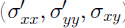
The first-order constitutive equations (Glen’s flow law) are:


where u, v are the horizontal velocity components in the x and y directions, respectively, m is an enhancement factor,
T is temperature and A is a temperature-dependent rate factor (Reference BlatterBlatter, 1995). The horizontal gradients of vertical velocity component are neglected in Equations (2c) and (2d) because they are of the second order.
The second invariant of the deviatoric-stress tensor, τe, in the first-order approximation (Reference HuybrechtsHuybrechts, 1992) is:

Velocity fields are calculated with surface and bedrock topography by the method of Reference BlatterBlatter (1995) with Equations (1–3). Then the local horizontal mass flux is obtained by vertical integration of the velocity fields, from which the evolution of the local ice thickness is determined.
The computation of the transient temperature field follows the method of the EISMINT models and considers horizontal and vertical ice advection but only vertical heat diffusion,

where cp and kI are the specific heat capacity and the thermal diffusivity of ice.
The first-order strain-heating term (Φ) is:

In the SIA, only the first two terms on the righthand side of Equation (5) are included.
The energy equation (4) is solved with prescribed surface temperature and geothermal heat flux  at the bottom boundary,


where Tpm is pressure-melting-point temperature.
The ice-stiffness (viscosity) coefficient, A = A(T), strongly depends on ice temperature, and velocity fields and temperature are coupled through this factor. The factor A is incorporated using an Arrhenius relation as follows:

where T' is absolute temperature corrected for the dependence of melting point on pressure (Reference PatersonPaterson, 1994). Parameters a and Q are given by the following relations (e.g. Reference HuybrechtsHuybrechts, 1992; Reference PaynePayne and others, 2000):


The computation of all other quantities corresponds to that in the SIA models.
3. Experiments and Results
The present work focuses on the effects of the horizontal normal deviatoric stress. The experiments in this work are performed using the framework of the EISMINT model intercomparison experiments (Reference PaynePayne and others, 2000). The quadratic model domain spans 1500 x 1500 km. The grid resolution is 25 km in both horizontal coordinate directions (corresponding to 61 x 61 grids). Surface mass balance Ms (ice accumulation/ablation rate) and surface temperature Ts are given as a function of the horizontal distance to the summit position alone:


where (x0, y0) = (0 km, 0 km) is the position of the summit, Tmin and ST are the surface temperature at the summit and the radial surface temperature gradient, respectively, and Mmax , Sb, and R el are a given upper limit for the accumulation rate, the radial mass-balance gradient and the radial distance of the equilibrium line from the summit, respectively. All the experiments in this work use flat-bed topography as the bottom boundary, and the effects of isostasy are ignored. Basal sliding is also neglected. The steady-state shape of this ideal ice sheet assumes radial symmetry, and the effect of horizontal shear stress is small, so the comparison between steady states of the FOA and SIA models primarily shows the effects of the longitudinal stress gradient.
The enhancement factor is m = 1 through all the experiments in this work. Parameters Tmin, ST, Sb, R
el and geothermal heat flux  are set at 238 K, 1.67 x 10⁻² K km– 1, 10–2 ma–1 km–1, 450 km and 42 mW m–2 , respectively, through all the experiments. All experiments are performed with both the SIA and FOA models. Experiments with the SIA model are labelled with suffix 0, and experiments with the FOA model with 1. The initial condition is no ice except where specified. All the experiments are run for at least 200 kyr. The time-step is 5 years for dynamics and 20 years for the temperature equation. It takes about a day to finish a 200 kyr calculation using the FOA model on a Hitachi SR8000 supercomputer, and about half an hour using the SIA model.
3.1 Thermomechanically uncoupled (isothermal) model
The experiments U are performed using the same boundary conditions as for the corresponding experiment A in Reference PaynePayne and others (2000); U1 and UC stand for FOA and SIA, respectively. The only difference is that the experiments are performed for A in Equation (2) set constant at 1.0 x 10⁻¹⁶ Pa–3 a–1, such that the computed temperature field does not affect the viscosity of the ice. The parameter Mmax is set at 0.5 m a–1, the same as in experiment A in Reference PaynePayne and others (2000).
Figure 1 shows the difference in the steady-state surface elevations of the U experiment. The effect of the first-order stress on surface elevation (or thickness) is small. Most of the interior parts are thicker by about 10 m in the FOA (0.1–0.6% of the total ice thickness), whereas near the margin the ice is thinner by 20m or more (-4%). It should be emphasized that the use of a coarse grid for numerical models leads to inaccuracy at some places such as the margin. EISMINT and the present paper serve as a comparison of different numerical methods and may not provide the correct solution. Therefore it cannot be concluded that the FOA is better than the SIA; this paper only discusses the differences between them.
Steady-state results of the isothermal experiments (U) for difference in surface elevation between the FOA and the corresponding SIA model. The x axis gives the distance from the centre point along the diagonal of the quadratic model domain.

Vertical profiles of flow or stress components near a divide and elsewhere are discussed by Reference PayneRaymond (1983), Reference RaymondReeh (1988) and Reference Dahl-JensenDahl-Jensen (1989a, Reference Dahl-Jensenb). Similar results are obtained in this work. Figure 2 shows the vertical profiles of the horizontal velocity component at half a grid distance away from the ice divide (note that staggered grids are used for calculation of the horizontal velocity) by experiments U1 and Uc. The horizontal velocity of U1 is larger than that of Uc near the surface, and smaller near the bed. However, the horizontal ice flux of the steady-state solutions at the same point must be equal in both experiments, because the boundary condition of surface mass balance in the present work is explicitly a function of the distance from the ice divide, independent of thickness. The smaller velocity of U1 at deeper layers dominates the effect of the faster upper layers, so the vertically integrated velocity of U1 is smaller than that of Uc. As a result, the FOA ice thickness is larger than the SIA ice thickness. The difference between the two experiments at one grid further away from the ice divide is similar to, but smaller than, that at the first grid.
Vertical profiles of radial velocity (u) at (12.5 km, 0 km) (half-grid from the divide). They axis gives the height normalized with ice thickness. Thick and thin lines are the results of U1 and Uc, respectively.

The difference in vertical profiles of horizontal velocity between the two models can be explained qualitatively in terms of stress profiles. Figure 3 shows the vertical profile of stress components one grid away from the ice divide. As discussed by Reference PayneRaymond (1983), Reference RaymondReeh (1988) and Dahl-Jensen (1989a, b), this profile is qualitatively similar for the entire interior region. The FOA force-balance Equation (1a) in two dimensions becomes
Vertical profiles of stress components (σxz, σxx) at (25km, 0km). They axis gives the height normalized with ice thickness. Thick and thin lines are the result of U1 and Uc, respectively. Solid and dashed lines for each thickness are σxz and σ'xx respectively. Note that for Uc , σ xx is neglected and set to 0.


In the SIA, the second term on the righthand side is neglected. Near the divide where the surface gradient is negative, the gradient of longitudinal deviatoric stress is positive (divergence flow). Thus,

which corresponds to Figure 3. The constitutive Equation (2c) in two dimensions is

At the bed, where  Equation (14) becomes

which is equivalent to the SIA formulation. At the bed, the horizontal velocity in the FOA is smaller than in the SIA (Fig. 2), because σxz of U1 is smaller than that of UC at the bed.
Near the surface, where σxz → 0, Equation (14) becomes

Since the SIA neglects the  term in Equation (16), ∂u/∂z approaches zero faster in the SIA than in the FOA. Thus, near the surface, the vertical profile of horizontal velocity is steeper in the SIA than in the FOA (Fig. 2).
In spite of minor differences in surface elevation, basal temperatures differ substantially near the divide. Figure 4 shows the difference in basal temperatures (in terms of temperature below local pressure-melting point) between the two experiments. Inclusion of the first-order stress gradients produces a warmer base below the summit by 1 K because of the differences in vertical advection (Fig. 5). Note that the result shows clearly that a “hot spot” (Reference Dahl-JensenDahl-Jensen, 1989a) below the divide is produced by the first-order model.
Steady-state results of the isothermal experiments (U) for difference in basal temperatures between the FOA and the SIA model. The x axis gives the distance from the centre point along the diagonal of the quadratic model domain.

Vertical profiles of vertical velocity (w) below the divide. They axis gives the height normalized with ice thickness. Thick and thin lines are the results of U1 and U0, respectively.

In these experiments, thermomechanical coupling is not performed, and the temperature differences do not affect the softness of ice. If the flow parameter A is made temperature-dependent, warmer ice than in the above experiments may cause higher velocities, and the ice may become thinner. In section 3.2, the effects of thermodynamic coupling are discussed.
3.2. Eismint experiments
In this subsection, A series experiments are performed using the same boundary conditions as for the corresponding Eismint experiments A in Reference PaynePayne and others (2000). Now thermomechanical coupling is applied. It may be concluded that the effects of inclusion of the first-order stress gradients do not change much in comparison to the isothermal experiments.
Figure 6 shows the difference in basal temperatures between the steady-state results of A, and Ac along the diagonal section. It can be divided into three regions based on the different effects of the first-order stress gradients: (1) basal temperatures of A, are higher near the ice divide; (2) they are lower away from the divide (50 < d ≤ 300 km); and (3) they are equal in the region at the pressure-melting point (300 km < d). The behaviour near the ice divide can be explained by the difference in the vertical advection term, as in the U series (“hot spot”).
Steady-state results of experiment A for difference in basal temperature between result of A1 and that of Ac. The x axis gives the distance from the centre point along the diagonal of the quadratic model domain.

The behaviour away from the divide is more complex. In this case, the difference in strain heating between A1 and Ac is large compared to the difference in strain heating of experiments U, though the effect of first-order stress gradients is qualitatively the same. The reason for this large difference in basal strain heating seems to be positive feedback of temperature and strain, which occurs only in thermomechanical coupling: a decrease of strain heating causes a decrease in temperature, which in turn leads to harder ice. The harder ice further leads to smaller strain rates, which further reduce strain heating. There is a slight difference for regions with basal pressure melting. The melting region of A is narrower by about 30 km.
For some regions, the large difference in basal strain heating has a more complicated explanation. It derives mainly from the difference in basal shear stress in the two models. Figure 7 shows the difference in basal shear stress components between A1 and Ac. Except for the region near the area of the pressure-melting point (0 < d ≤ 150 km), the basal shear stress of A, is smaller than that of Ac. Since strain heating is the product of stress and strain rate, strain heating is reduced in this region. However, the region is characterized by higher shear stress as well as lower strain heating. The temperature is low enough that shear strain rate becomes small enough to cancel the effect of higher shear stress for strain heating. Further detailed analysis is required to clarify the feedback loop of thermomechanical coupling in this area. It may be due to the (small) difference in temperature advection from upper layers.
Difference in basal vertical shear stress between steady-state solutions of experiments A1 and Ac. The x axis gives the distance from the centre point along the diagonal of the quadratic model domain.

The steady-state surface elevation is affected by a temperature difference. However, the effect of the first-order stress gradients on the steady-state shape is small. Figure 8 shows the difference in surface elevation between A1 and Ac. The effect of the first-order stress on surface elevation is generally the same as in the isothermal experiment U. There is a slightly different behaviour near the divide, where the surface elevation is lower in the FOA than in the SIA, due to thermomechanical coupling (see section 3.1). Warmer ice near the divide results in softer ice, ice flow becomes faster, and consequently the ice sheet becomes thinner.
Steady-state results for difference in surface elevation between A1 and Ac. The horizontal axis gives the distance from the centre point along the diagonal of the quadratic model domain.

3.3. Diagnosis of age profiles below a steady-state summit
The vertical age profile at the ice divide (horizontal velocity = 0) of the steady-state ice sheet is computed by integrating the reciprocal of the vertical velocity component along the vertical axis to the surface:

In a steady state, the downward distance an ice particle moves in 1 year is equal to vertical velocity w; thus Equation (17) is obtained. It is assumed that the surface mass balance remains unchanged throughout the time integration. The region near the bed, where vertical velocity approaches zero (its reciprocal becomes infinite), is not considered. In this subsection, Z series experiments are performed using the same boundary conditions as in the corresponding experiments A in Reference PaynePayne and others (2000) except that the accumulation is reduced to 10% of the accumulation in experiments A.
Figure 9 shows the results of age calculations at the ice divide of experiments A and Z. The differences gradually increase toward deeper parts. The accumulation of experiment A is 50 cm a–1, a typical value for Greenland drilling sites, and the accumulation of experiment Z is 5 cm a–1, a typical value for Antarctic drilling sites. At 2000 m depth, the age of the ice in experiment Z1 is 130 kyr, while in Zc is 120 kyr. The difference is as much as 10 kyr (-10% of age). At 3000 m depth, the age of the ice in experiment A1 is 18 kyr, while that in experiment Ac is 16 kyr. The difference is as much as 2 kyr (~10%). In this case, the vertical velocity components at both surface and base boundaries must be the same for both approximations because of the prescribed boundary conditions. The largest difference occurs at middle depth where the vertical velocity in the FOA is slower than that in the SIA at the same depth (Fig. 5), as previously discussed in Reference PayneRaymond (1983), Reference RaymondReeh (1988) and Reference Dahl-JensenDahl-Jensen (1989a).
Vertical profiles of age of the ice below the ice divide of experiments A (a) and Z (b). They axis gives the depth below the ice surface. Thick and thin lines are the results of the FOA and SIA models, respectively.

This is the case for such an idealized configuration. In the case of realistic ice sheets with surface elevation, velocity profiles and surface accumulation changing through time, the difference in the calculated age of the ice may be considerably larger.
4. Conclusion and Prospects
In the present work, a three-dimensional numerical ice-sheet model with thermodynamic coupling including the first-order mechanics is presented. The model is applied to an idealized ice sheet with radial symmetry to investigate the effects of the normal deviatoric-stress gradients on ice thickness, basal temperature and age distribution. The main conclusions of the present work are as follows:
The difference in age profiles below the steady-state summit between the FOA and the SIA reaches as much as 10% of total age near the base.
Basal temperature differs as much as ± 1 K between the FOA and the SIA, due either to the difference in the vertical advection (near the divide) or to the difference in strain heating (away from the divide).
The difference in surface elevation of steady states between the FOA and the SIA models is generally small (only a few tens of metres).
The insignificant differences between the results obtained by the FOA and SIA models are due to the simple configuration of the experiments. Because of the flatbed and the radial symmetry, the role of higher-order stress components is expected to be small in almost the whole domain. The implications of the present work are limited, and it cannot be concluded from the present result alone that the FOA model is better than the SIA model. However, careful interpretation of the simulated flow and geometry of ice sheets is required in certain cases, because of the different characteristics of the two models.
In addition to the idealized study presented, several applications of the first-order model developed in the present work are planned for the future. Firstly, the presented FOA model can be used for dating. Secondly, it can be an effective tool to connect ice microphysics to large-scale ice-sheet behaviour. Thirdly, it can be used to study ice-stream dynamics. In addition, basal sliding, which is also important for ice-stream dynamics, may present different behaviour in the two approximations, due to the difference between the basal shear traction, used in FOA models, and the driving stress, used in SIA models, to parameterize sliding. Therefore, studies on the stability of marine ice sheets such as the West Antarctic ice sheet require the application of the FOA model; this is a planned future application of the presented model.
Acknowledgements
The authors wish to thank L.W. Morland, the editor, and two anonymous reviewers for their useful comments.



