Introduction

One of the major factors which determine the flow of an ice shelf is its tempcrature, T, through its influence on the flow parameter in the Arrhenius equation A(T') =A_o exp(-Q/RT'). A_o represents a constant, R is the gas constant, T' is the absolute temperature and Q is the activation energy. The temperature distribution within an ice shelf depends on the temperature at the ice surface, the water temperature at the ice-shelf bottom, the accumulation and melting rates, and the temperature distribution within the ice streams discharging into the ice shelf These environmental conditions vary at different regional and local situations. Consequently, thc ice body produces local and regional structural features. These tCatun's are illustrated in the Glaciological Map of Filchner-Ronne Ice Shelf (Swithinbank and others, 19(8). In addition, the distributions of meteoric and marine ice were determined from radio-echo sounding and elevation measurements in the central part of Filchner-Ronne Ice Shelf and were compiled together with recognizablc structural marks derived from airborne RES byReference Thyssen, Bombosch and hagerThyssen and others (1992). In both maps, a zone of “ chaotic disturbed” or “ destroyed meteoric ice” northeast of Henry Ice Rise is described. Diffraction hyperbolas, found in high-resolution RES measurements (Reference Blindow, Miller and OerterBlindow 1991), follow distinct f10wlines which partly originate in this area (B1indow, 1994). One reason for the crcvassing is the grounding zonc of Henry Ice Rise (see Fig. 1). Another reason is the formation of the marine ice layer due to crystallization processes in the water column beneath the central part of Filchner Ronne Ice Shelf (Reference Thyssen and KohnenThyssen 1986, Reference Swithinbank, Brunk and Sievers1988, Reference Blindow, Miller and Oerter1991); (Reference Engelhardt and DetermannEngelhardt and Determann 1987); (Reference OertelOertel' and others 1992).

Fig. 1.

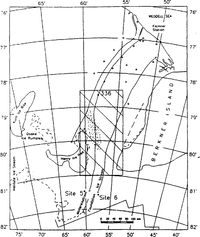
Flowlines for the thermal modeling, geodetic points (Reference Moller, Riedel, Ritter and OertelMoller and others 1992)and location of the data base for local dynamic model calculations (rectangular box in middle of figure). The disturbed ice is marked with a dotted field (map from (Reference Swithinbank, Brunk and SieversSwithinbank and others 1988).

The area of marine ice covered by this study is limited by Rutford Ice Stream in the west, Korff Ice Rise and Henry Ice Rise with Doake Ice Rumples in the south and Foundation Ice Stream in the east (Reference Thyssen, Bombosch and hagerThyssen and others 1992),

Heat advection due to marine accumulation is the main reason for the increase of the ice temperature and therefore for the flow parameter. Spatially varying flow parameters derived from the vertical temperature distributions observed in boreholes and thermal model calculations along selected flowlines, assuming steady state (Reference GrosfeldGrosfeld 1992), arc employed in two-dimensional flow simulations. This leads to a local maximum of vertically integrated temperature which is calculated to occur north and northeast of Henry Ice Rise between 150 and 200km along the flowline downstream of Mbllereisstrom (Reference GrosfeldGrosfeld 1992). We therefore have a condition of confined flow between Henry Ice Rise and Berkner Island coupled with horizontal temperature variations. In this paper a local flow simulation with a horizontally varying 110w parameter is compared with conventional calculation using a constant flow parameter.

Theory

Model calculations on Filchner-Ronne Ice Shelf with two dimensional finite-clement methods (Reference Lange and MacAyealLange and MacAyeal 1986 1988), or finite-difference methods. (Reference DetermannDetermann 1991 a) were conducted on a Filchner-Ronne Ice Shelf data base. We used a versatile finite-difference method, developed for local data bases with high resolutions. For the descriptions, λ, ɸZ are used as coordinates on a polar stereographic projection, x, y, z as position componen ts and u, v, w as velocity components. Flow simulations are based on the numerical solution of the momentum equations under ice-shelf conditions. With stress tensor a, ice density p, gravitational acceleration 9 and vertical unity vector k, neglecting inertial forces and the Coriolis force, the equation of motion can he written Reference Lliboutry(Lliboutry 1987); as

The generalized flow law for incompressible material: (Reference Jaeger(Jaeger 1969): E^xy= Aσ ^n-1σ ¹ _xywith ϶ _xycomponents, ϶¹ _xy the stress-deviator components, ϶the effective stress,n the flow-law exponent (n = 3) and A the flow parameter, depending on temperature T Reference Paterson(Paterson 1981), describes the relation between deformation rate and the stress tensor.

Looking at the ice-shelf flow as deforming ice columns, vertical shear is negligible (Reference SandersonSanderson and Doakc 1979), so that δ ϶ ¹ _xy/δ x, δ ϶ ¹ _yZ δ y = O.A vertically integrated flow parameter

can be derived from temperature distribution. Vertical deformation can be taken into account by using ice equivalent for vertical density variation (Reference ThyssenThyssen 1988). The velocity change with flow parameter is considered in the flow law with u, v, w as velocity components

using Equations (2) and (3), the elliptic differential equations of second order can be solved with the surface elevation gradients δz/δx, δz/δy to:

With δu/δz, δv/δz;͌0 and δw/δx, δw/δy, «δu/δx, δv/δy, 1and the effective strain rate is calculated:

The velocity components were approximated with difference forms of Equations (2) and (3), comparable to diagnostic procedures described by (Reference DetermannDetermann 1991 b). Looking at the approximated velocity components as dilatation parameters, principal strain rates were calcul-ated to compare with geodeticall . rates. ϶_1,2=1/2(϶_XX+ ϶yy ± ē) with e=(϶xx - ϶yy)² + 4϶_xy (Reference Moller, Riedel, Ritter and OertelMoller and others 1992). The vertical strain rate ϶_zz = -(϶: + ϶yy) = -(e1 + e2) can be determined as invariant under transformation of the coordinate system. Together with the flow law, stress-deviator components can be calculated with σ¹ _jj = ϶ij A^-1/n϶ ^l-(1/n).

The theoretical basis of the temperature calculation is heat conduction and advection with thermal properties, depending on density, salinity and temperature. The method has been described in detail for the flowline downstream of Mollereisstrom by Grosfeld and Thyssen (1994). The vertical temperature distribution T(λɸᴢ) is calculated using ice thickness H = H_meteoric + H_marine, velocity, melting and freezing rate, and top and bottom temperature at 2km grid intervals along the flowlines in Figure 1and equidistant vertical increments between 4 m and ahout 1m. These temperature values were used to calculate the appropriate flow parameter (Reference PatersonPaterson 1981)and vertically integrated to get Ā (λ, ɸ), which was transformed to the x, y coordinate system. For the dynamic simulation, this Dow parameter A(x, y) and the ice thickness H(x, y) are used as input data.

Data bases and results

An interactive program system was created on a personal computer to approximate velocity components at each grid point using a finite-difference relaxation method and to calculate the strain-rate components and stressdeviator components. In the central part of Filchner Ronnc Ice Shelf, ice-thickness distributions H, H _meleoric and H _marinc have been derived from airborne RES measurements together with elevation measurements along flight tracks (Reference Thyssen, Bombosch and hagerThyssen and others, 1993). Twodimensional data sets were calculated by mathematical tool programs for gridding and in terpola tion. Tce thickness, constructed in the central area with grid distances of 10km in the x direction and ]3 km in the y direction, was used for regional model calculations with an average flow parameter af A =7.5 X 10^-18 Pa^-3 a^-1 (Reference DetermannDetermann 1991a) to derive the boundary conditions for the local grid. The results are shown in Figure 2.

Fig. 2.

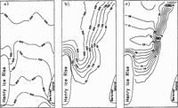
Velocities in m a ¹ of regional calculation for the boundary values (map from Swithinbank and others, 1988).

Compared to the results of Reference DetermannDetermann (1991a), the velocities are decreased due to boundary conditions which consider two components of the strain rate at the ice front (Reference HuybrechtsHuybrechts 1992). Thus, deviations of grid-point positions from the actual coastline may decrease the accuracy of the model results. The model predictions are in reasonable agreement with the geodetically measured velocities. Near site 5 Fig. 1, the results show velocities between 100 and 200 m a^-1 compared to 170 Reference Ritter and Karsten(Ritter and Karsten 1991) and 198.5m a^-1 Reference Morris, Vaughan, Miller and Oerter(Morris and Vaughan, 1991). At point 336, the model velocity reaches 600 m a^-1, where 660 m a^-1.Reference Moller, Riedel, Ritter and Oertel(Moller and others 1992)was measured.

Downstream of Mollereisstrom and Foundation Ice Stream, the data base for an area between Henry lee Rise and Berkner Island, 140km wide and 280km long, was prepared. It is marked in Figure 1 together with the flowlines used for modeling of (T(λɸ)(Reference Thyssen, Bombosch and hagerThyssen and others 1993); (Reference Grosfeld and ThyssenGrosfeld and Thyssen 1994). The data bases of ice thickness and flow parameter are converted to grid distances of 1.4 km. They are shown in Figure 3 together with the thickness of the marine-ice layer in this area. The derived integrated flow parameter at Foundation Ice Stream, where no basal freezing has been detected, ranges between 4.4 x 10 ¹⁸ and 7.5 x 10 ¹⁸Pa^-3 a^-1, corresponding to temperatures between -22.5° and -17.5°C. In the area of marine ice, A varies from 1 x 10^-17 to 3.5 X 10^-17 Pa^-3a^-1, which corresponds to average temperatures between -15° and -7.5°C.

Fig. 3.

Data bases of (a) ice thickness H (m), (b) marine-ice thickness H _marinp (m) (Thyssen and others, 1993) and (c) flow parameter (x 10 ¹⁸ Pa ³ a 1).

A local maximum of 3.3 x 10^-17 Pa^-3 a^-1 is reached north and northeast of Henry Ice Rise. As expected, the flow parameter reaches a local maximum in this area of basal freezing, (Reference Grosfeld and ThyssenGrosfeld and Thyssen 1994).

On the: loe:al domain, two diagnostic simulations were performed. In the first simulation, a spatially variable flow parameter was used. The second one was calculated with the constant-fIow parameter of Ā=7.5 x 10 ¹⁸ Pa^-3 a ¹ to get the results on the same grid size. Velocities from both simulations together with the difference are plotted in Figure 4. , Even though the boundary values remain unchanged, the difference increases to 14 ma¹ in the reg-ion of basal freezing.

Fig. 4.

Velucities in mal of calculation with (a) A(T(x,y »(Fig. 3c), (b) constant-flow parameter qf 7.5 x 10^-18pa^-3 a^-1, (C) difference between (a) and (b).

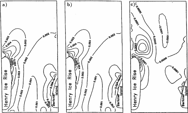
The principal strain rate a₁ at point 336 is measured as 0.0022a^-1, (Reference Ritter and KarstenRitter and Karsten 1991). The calculated principal strain rates a¹ are show in in Figure 5. In the region of point 336 they reach values between 0.002 and 0.003 a¹ .Measured and calculated strain rates are

Fig. 5.

Prinripal strain rates e₁ (a ^-1) of calculation with (a) A(T(x, y))(Fig. 3c), (b) constant-flow parameter of 7.5 x 10^-18pa ³ a^-1, (c) difference between (a) and (b).

comparable in magnitude. The diJTerences are caused by the boundary velocity field and its deviations from measured velocity as described above. The highest values are reached in the grounding zones, decreasing to the region of free-floating ice. The difference diagram shows a local maximum of 0.0004 a^-1 northeast of Henry Ice Rise. The contribution of the spatially varying flow parameter can be estimated as up to 10%.

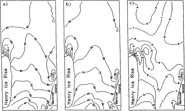
The situation is similar, when looking at the vertical strain rate:s (Fig. 6). A local maximum can be seen northeast of Henry Ice Rise. I t is enlarged in the diagram of the spatially varying flow parameter. This area can be identified with the crevassed area (seeFig. 11.) Crevassing in this area takes place at the surface. So the temperature of the meteoric ice must be taken into account for the calculation of the stress components. The principal stress as in Figure 7 is calculated using a flow parameter of 5.7 x 10 ¹⁸ Pa ³ a ¹. The contribution of the temperature increase can be estimated when looking at the differences between the calculation using constant A and lateralvarving A(T(x,y)), which is locally increased here. Critical values for crevasses are given as greater than 100 kPa(Reference WeertmanWeertmann 1980).They are reached northeast of Henry Ice Rise, if a temperature appropriate to nearsurface ice of 20°C is considered.

Fig. 6.

Vertical strain rates ϵzz (a^-1) of calculation with (a) A(T(x, y)) (Fig. 3c), (b) constant-jlow parameter of 7.5 x 10 ¹⁸ Pa³a^-1, (c) difference between (a) and (b).

Fig. 7.

Near-surface stress component σ₁ (kPa) 0f calculation with (a) constant-flow parameter of 7.5 x 10 ^-18 Pa^-3a ¹, (b) A(T(x, y)) (Fig. 3c), (c) difference between (a) and (b).

Conclusions

The radio-echo-sounding work In the central area of Filchner-Ronne Ice Shelf revealed new information on total ice thickness, meteoric and marine-ice thickness and structural features. These data give information about regional and local situations in more detail and represent a broad base for experimental and numerical procedures. This paper deals with the zone of disturbed ice northeast of Henry Ice Rise. In this area, the values of velocity and vertical strain rates calculated using the spatial-varying flow parameter are up to 10% higher than the values obtained by using a constant-flow parameter. The maxima are situated northeast of Henry Ice Rise. This can be identified with the crevassed area from the satellite map (Reference Swithinbank, Brunk and SieversSwithinbank and others 1988) and the feature map from, Reference Swithinbank, Brunk and Sievers Thyssen and others (1993). The increase in the temperature field due to basal accumulation leads to an enlarged zone of increased vertical strain and accentuates crevassig.

Acknowledgement

The authors wish to express their thanks to the Deutsche Forschungsgemeinschaft,