1. Introduction
When a shock wave impulsively accelerates an interface separating two fluids of different density, initial perturbations on the interface first grow linearly, then nonlinearly over time. In the nonlinear regime, the interface undergoes substantial distortion, with the spikes (heavy fluid penetrating into light fluid) and bubbles (light fluid rising into heavy fluid) growing asymmetrically, which may eventually trigger the transition to turbulent mixing. This type of hydrodynamic instability is referred to as the Richtmyer–Meshkov instability (RMI) (Richtmyer Reference Richtmyer1960; Meshkov Reference Meshkov1969). A similar but distinct instability is the Rayleigh–Taylor instability (RTI), which occurs as the interface is subjected to a sustained acceleration (Rayleigh Reference Rayleigh1883; Taylor Reference Taylor1950). The RMI exists widely in scientific and industrial fields with length scales spanning from millimetres (e.g. inertial confinement fusion, ICF) (Murakami & Nishi Reference Murakami and Nishi2017; Li, Samtaney & Wheatley Reference Li, Samtaney and Wheatley2018) to light years (e.g. supernova explosions) (Kuranz, Park & Huntington Reference Kuranz, Park and Huntington2018). For example, during ICF implosions, RMI develops at both the exterior ablator–shell interface and the interior shell–fuel interface (Haan, Lindl & Callahan Reference Haan, Lindl and Callahan2011; Casey, Smalyuk & Tipton Reference Casey, Smalyuk and Tipton2014; Samulski, Srinivasan & Manuel Reference Samulski, Srinivasan and Manuel2022; Li, Yan & Zhao Reference Li, Yan and Zhao2022; Abu-Shawareb, Acree & Adams Reference Abu-Shawareb, Acree and Adams2024), significantly enhancing mixing between the outer ablator and inner fuel. Such undesired mixing greatly degrades energy yield and may even lead to ignition failure (Lindl, Landen & Edwards Reference Lindl, Landen and Edwards2014). In contrast, in scramjet engines, RMI-enhanced mixing between fuel and air is beneficial for improving combustion efficiency (Urzay Reference Urzay2018; Wu, Li & Lu Reference Wu, Li and Lu2024; Bajaj, Kansara & Nath Reference Bajaj, Kansara and Nath2025). The underlying mechanisms of conventional RMI are primarily baroclinic vorticity and pressure disturbance. Specifically, during shock–interface interaction, the misalignment between the pressure gradient
 $\boldsymbol{\nabla}p$
across the shock and the density gradient
 $\boldsymbol{\nabla} \rho$
at the interface (
 $\boldsymbol{\nabla \!}\rho \times \boldsymbol{\nabla \!}p$
) gives rise to baroclinic vorticity, which in turn drives the interface deformation. Meanwhile, the shock induces pressure disturbances that create local pressure differences along the interface, contributing to perturbation growth (Zabusky Reference Zabusky1999; Brouillette Reference Brouillette2002; Zhou, Sadler & Hurricane Reference Zhou, Sadler and Hurricane2025).
The RMI at gas/gas interfaces and the resulting turbulent mixing have been extensively studied through experiments (Jones & Jacobs Reference Jones and Jacobs1997; Sadot, Erez & Alon Reference Sadot, Erez and Alon1998; Jacobs & Krivets Reference Jacobs and Krivets2005; Balakumar, Orlicz & Tomkins Reference Balakumar, Orlicz and Tomkins2008; Morgan, Aure & Stockero Reference Morgan, Aure and Stockero2012; Balasubramanian, Orlicz & Prestridge Reference Balasubramanian, Orlicz and Prestridge2012; Mohaghar, Carter & Pathikonda Reference Mohaghar, Carter and Pathikonda2019; Mansoor, Dalton & Martinez Reference Mansoor, Dalton and Martinez2020; Noble, Ames & McConnell Reference Noble, Ames and McConnell2023), simulations (Youngs Reference Youngs1994; Latini, Schilling & Don Reference Latini, Schilling and Don2007; Youngs & Williams Reference Youngs and Williams2008; Thornber, Drikakis & Youngs Reference Thornber, Drikakis and Youngs2010; Hahn, Drikakis & Youngs Reference Hahn, Drikakis and Youngs2011) and theoretical analyses (Zhang & Sohn Reference Zhang and Sohn1997; Mikaelian Reference Mikaelian2005; Dimonte & Ramaprabhu Reference Dimonte and Ramaprabhu2010; Zhang, Deng & Guo Reference Zhang, Deng and Guo2018; Soulard & Griffond Reference Soulard and Griffond2022). For a comprehensive overview on this topic, readers are referred to several existing reviews (Zabusky Reference Zabusky1999; Brouillette Reference Brouillette2002; Ranjan, Oakley & Bonazza Reference Ranjan, Oakley and Bonazza2011; Zhou Reference Zhou2017a , Reference Zhoub ; Zhou et al. Reference Zhou, Sadler and Hurricane2025). The RMI at gas/liquid interfaces is relevant to high-pressure diesel injection, where shock–spray interactions influence droplet breakup and the bubble–fuel dynamics (Liang, Jiang & Hu Reference Liang, Jiang and Hu2023). Early shock–droplet experiments (Lane Reference Lane1951; Nicholls & Ranger Reference Nicholls and Ranger1969) showed that convective shearing dominates over RMI. Experimental challenges in generating stable gas/liquid interfaces have thus limited systematic studies, while theoretical analyses indicated that viscosity suppresses instability growth (Mikaelian Reference Mikaelian1993; Carlès & Popinet Reference Carlès and Popinet2001, Reference Carlès and Popinet2002; Mikaelian Reference Mikaelian2019). The RMI at gas/solid interfaces poses unique observational challenges but has been established as a diagnostic tool for material strength. Early radiographic studies (Barnes, Blewett & McQueen Reference Barnes, Blewett and McQueen1974) demonstrated the role of dynamic yield strength in perturbation evolution, while later X-ray and interferometric measurements (Jensen, Cherne & Prime Reference Jensen, Cherne and Prime2015; Prime et al. Reference Prime, Buttler and Buechler2017, Reference Prime, Buttler and Fensin2019) linked spike velocities to strength in various metals. On the theoretical side, empirical and analytical models (Piriz, López Cela & Tahir Reference Piriz, López Cela and Tahir2006; Dimonte, Terrones & Cherne Reference Dimonte, Terrones and Cherne2011) have provided predictive frameworks for the perturbation dynamics in elastoplastic solids.
Another important class of interfaces that has received relatively little attention is that involving viscoelastic materials. Dimonte, Gore & Schneider (Reference Dimonte, Gore and Schneider1998) examined RTI in yogurt, a material with well-characterised mechanical properties (shear modulus, yield stress, viscosity), and precisely measured the critical wavelength and amplitude. Later, Mora, Phou & Fromental (Reference Mora, Phou and Fromental2014) experimentally and theoretically demonstrated a gravity-driven RTI in soft elastic solids, finding that under some conditions the initially flat surface destabilises into steady patterns. Chakrabarti, Mora & Richard (Reference Chakrabarti, Mora and Richard2018) demonstrated that a soft elastic slab under gravity buckles into a hexagonal pattern via a discontinuous transition. Zheng, Lai & Hu (Reference Zheng, Lai and Hu2019) further reported that lateral confinement of elastic soft gels within a rigid cylindrical container not only increases the critical load for instability but also alters the resulting patterns. Some progress has also been made in the theoretical analyses of viscoelastic RTI (Tan & Wang Reference Tan and Wang2019; Liu Reference Liu2023). Compared with viscoelastic RTI, viscoelastic RMI remains largely unexplored. A few theoretical studies, such as the extension of Goncharov’s model (Goncharov Reference Goncharov2002) to viscoelastic fluids by Rollin & Andrews (Reference Rollin and Andrews2011), have revealed that viscoelasticity alters both linear growth and the late-time dynamics. However, these predictions remain unvalidated, as no experiments on viscoelastic RMI have yet been conducted under controlled initial conditions. The primary challenge lies in the difficulty of precisely controlling both the mechanical properties of viscoelastic materials and the initial interface shape, since these materials typically exhibit strong rate-dependent, nonlinear and history-dependent behaviours. Furthermore, the evolution mechanisms of viscoelastic RMI are inherently complex, involving the interplay of viscous dissipation and elastic energy storage, making purely theoretical analyses insufficient to capture the full range of phenomena. It is therefore highly desirable to perform high-fidelity experiments on viscoelastic RMI under controlled initial conditions. Such experiments would not only enable rigorous validation of existing theoretical models but also reveal new physical mechanisms, thereby guiding the development of more accurate predictive models. This motivates the present study.
Compressibility plays a crucial role in RMI at different types of interfaces, particularly at very early times. Richtmyer (Reference Richtmyer1960) first proposed a compressible linear theory, which was later extended by Wouchuk & Nishihara (Reference Wouchuk and Nishihara1996) to an exact formulation valid under general compressibility conditions. Lombardini & Pullin (Reference Lombardini and Pullin2009) further showed that, unlike the instantaneous onset predicted by impulsive models, the growth rate starts from zero and rises toward a linear asymptote over a characteristic time scale. For the nonlinear stage, Zhang et al. (Reference Zhang, Deng and Guo2018) introduced a unified compressible framework linking early-time linear growth with the late-time nonlinear dynamics, which was later extended by Zhang & Guo (Reference Zhang and Guo2022) into a comprehensive model for spike and bubble evolution. Most of these theories were developed under the ideal-gas equation of state (EoS), whereas viscoelastic RMI often involves non-ideal EoS. Although fitted ideal-gas models have been used in high-energy-density experiments (Dimonte & Remington Reference Dimonte and Remington1993; Holmes, Dimonte & Fryxell Reference Holmes, Dimonte and Fryxell1999), they do not necessarily reproduce shock-front oscillation frequencies and decay rates (Endo, Shigemori & Azechi Reference Endo, Shigemori and Azechi1995). To address this, compressible theories based on non-ideal EoS have been developed. Cobos Campos & Wouchuk (Reference Cobos Campos and Wouchuk2014) derived analytic asymptotic velocities for weak and strong shocks. More recently, Napieralski, Cobos & Velikovich (Reference Napieralski, Cobos and Velikovich2024) proposed a fully compressible analytic theory for reflected-shock RMI under arbitrary EoS, solving the initial-value problem via direct inverse Laplace transforms. Numerical investigations using the Mie–Grüneisen EoS (Ward & Pullin Reference Ward and Pullin2011) revealed that EoS choice can strongly affect RMI growth, particularly in reflected-shock scenarios.
In this work, we shall systematically investigate RMI at gas/viscoelastic interfaces via shock tube experiments. Hydrogels with precisely controlled compositions and concentrations are employed to produce viscoelastic materials with tuneable mechanical properties, ranging from highly viscous to predominantly elastic. High-speed imaging captures the temporal evolution of interface perturbations, encompassing both small-amplitude, short-wavelength modes and large-amplitude, long-wavelength deformations. Detailed analyses of interface morphology, amplitude growth and oscillation behaviour reveal the fundamental mechanisms governing viscoelastic RMI. To characterise viscoelastic effects, we develop a new linear theoretical model based on the Maxwell framework, which incorporates both viscous dissipation and elastic energy storage. Although our model is based on the incompressible-flow assumption and therefore cannot capture the very early-stage dynamics, it reproduces the experimental observations with good accuracy. Moreover, it quantitatively reveals how the interplay between viscosity and elasticity governs the growth and oscillation of the initial perturbations.
2. Experimental methods
The experiments are performed in a horizontal shock tube at the Shock Wave Laboratory, University of Science and Technology of China. Hydrogel is selected as the test material due to its unique microstructure and tuneable viscoelastic properties. Specifically, it comprises two primary components: a three-dimensional (3-D) network of interconnected colloidal particles, which provides elastic behaviour, and an aqueous medium (water) filling the structural voids, which contributes to viscous properties. This distinctive composition endows hydrogels with mechanical properties intermediate between solids and fluids, making them an ideal material for systematically investigating the interplay between elastic and viscous effects during shock–interface interactions. A rigorous preparation protocol is employed to ensure reproducibility and precise control of material properties, as illustrated in figure 1(a). The process begins with the uniform dispersion of carrageenan or agar powder in distilled water at controlled concentrations. The mixture is then heated to
 $100\,^{\circ }\mathrm{C}$
using a magnetic stirrer heater, ensuring complete dissolution and homogeneous distribution of the polymer. Subsequently, the heated solution is poured into pre-prepared moulds with specific geometries (constructed of a carved acrylic border and a peel-off silicone pad), and cooled at room temperature for 1.5 h, during which the polymer network forms and the hydrogel solidifies. During the cooling process, carrageenan molecules transition from a disordered state at elevated temperatures to a helical configuration, ultimately forming a well-organised 3-D network. By varying the polymer type (carrageenan vs. agar) and concentration while maintaining consistent experimental conditions, hydrogels with tailored viscoelastic properties can be reproducibly fabricated. This preparation method offers two key advantages: (i) precise control over material composition through polymer concentration adjustment, which allows for effective tuning of viscoelastic properties; (ii) tunability of viscoelastic boundary geometry through mould design, enabling the formation of air/viscoelastic interfaces with desired shapes. To ensure consistent and reproducible properties, all polymer powders used in the present experiments are sourced from a single factory lot, thereby largely eliminating potential variability between different lots.
Schematic diagrams of (a) the hydrogel moulding process and (b) the experimental optical path.

In experiments, a hydrogel block is placed in the test section of the shock tube. This block is pre-fabricated with a sinusoidal interface at one end to serve as the seed for RMI. The interface shape in Cartesian coordinates is given by
 $y=a_0$
cos(
 $2\pi x/\lambda$
), where
 $a_0$
is the initial perturbation amplitude and
 $\lambda$
is the perturbation wavelength. In this study,
 $a_0$
is set to 1 mm and
 $\lambda$
to 17.5 mm, corresponding to an amplitude-to-wavelength ratio of 0.057. This ratio is carefully chosen to be sufficiently small to satisfy the small-perturbation assumption commonly used in linear stability analysis, while remaining large enough to facilitate clear visualisation and accurate measurement of interface evolution. Note that the hydrogel block features two distinct interfaces in the shock propagation direction: the sinusoidal interface for initiating RMI, and a planar interface on the opposite end. These interfaces are separated by 115 mm, a distance sufficient to prevent interface coupling effects within the experimental time scale. Initially, the hydrogel is placed in an acrylic box, with its cross-sectional dimensions matching those of the box. Although the hydrogel is not adhered to the test section, friction between the hydrogel and the test section is present. Following shock impact, the hydrogel slides within the box, with a measured sliding distance of approximately 63 mm. Due to the substantial density contrast between air (1.29 kg m
 $^{-3}$
) and hydrogel (approximately 1000 kg m
 $^{-3}$
), the incident shock is primarily reflected at the interface, with only a weak transmitted shock propagating into the hydrogel. This weak transmission, combined with the large separation distance between interfaces, ensures that waves reflected from the planar interface have negligible influence on the RMI at the sinusoidal interface. The test section is designed to approximate 2-D flow conditions: the inner height of the test section (i.e. the hydrogel block height) is only 6 mm, much smaller than its width (120 mm) and length (115 mm). This configuration effectively suppresses 3-D effects, ensuring that the interface evolution can be analysed within a 2-D theoretical framework, as outlined in § 4.
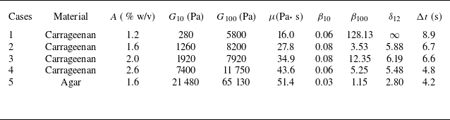
Rheometer measurements of hydrogel material properties under varying experimental conditions. Here,
 $A$
represents concentration, calculated by dividing the mass of the solute by the volume of the solvent,
 $G$
represents the shear modulus, with subscripts indicating the applied strain rate and
 $\mu$
denotes viscosity, which is measured at a strain rate of 10 rad s–1. The loss factor
 $\beta$
includes subscripts to indicate the corresponding strain rates during testing and
 $\delta _{12}$
represents the amplitude decay ratio between the first and second peaks, while
 $\Delta t$
denotes the time interval between these peaks.

In experiments, hydrogels with varying concentrations are prepared, and their rheological properties are characterised by the loss factor measured by a rheometer. The loss factor, defined as the ratio of the loss modulus
 $G^{\prime \prime }$
to the storage modulus
 $G^{\prime }$
in dynamic rheometer tests (
 $\beta =G^{\prime \prime }/G^{\prime }$
), provides insight into the material’s rheological behaviour. A higher loss factor indicates viscosity dominance, while a lower value suggests elasticity dominance. Specifically, the material behaves as a viscous fluid when
 $ \beta \gg 1$
, as an elastic solid when
 $\beta \ll 1$
, and exhibits a balance between viscous and elastic effects when
 $\beta \approx 1$
. Table 1 summarises the rheometer data for cases 1–5, which differ in polymer type (carrageenan vs. agar) and concentration. The significant differences between
 $\beta _{10}$
and
 $\beta _{100}$
, where the subscripts denote the strain rates applied during testing, indicates a pronounced strain-rate dependence of the hydrogel’s rheological properties. At low strain rates (10 rad s−1), the loss factor remains relatively constant across different concentrations, whereas at higher strain rates (100 rad s−1), significant variations are observed. This strong strain-rate sensitivity complicates the analysis of the present experimental results, where the strain rates are both high and time-dependent. Moreover, the hydrogel’s response to dynamic loading involves complex mechanisms such as polymer chain reorganisation, water migration within the network and potential structural damage, none of which are captured in steady-state rheometer measurements. Therefore, while the measured data serve as a useful reference, they do not fully represent the material properties under shock loading conditions.
High-speed photography is employed to directly capture interface evolution, as illustrated in figure 1(b), instead of using schlieren or shadowgraph techniques. This approach is chosen for two main reasons: first, the large difference in light transmittance between hydrogel and air enables direct imaging with good contrast; second, the water marks left by the sliding hydrogel block on the acrylic walls would interfere with schlieren or shadowgraph visualisation. While this method offers clearer interface visualisation with improved contrast and minimal surface artefacts, it cannot resolve the wave system. To compensate for this limitation, a series of shadowgraph experiments involving a planar shock wave interacting with a gas/hydrogel interface is conducted to accurately determine the incident shock conditions. The high-speed camera operates at a frame rate of 10 000 frames per second with an exposure time of 1
 $\unicode{x03BC} \mathrm{s}$
. The spatial resolution of the schlieren images is approximately 0.17 mm pixel−1. By maintaining a constant pressure ratio between the driver and driven sections of the shock tube, all tests achieve a consistent shock Mach number of
 $1.29 \pm 0.04$
.
3. Results and discussions
3.1. Interface morphology evolution
Figure 2 illustrates the evolution of the single-mode air/hydrogel interface accelerated by a planar shock for cases 1, 2, 4 and 5. The interface behaviour in case 3 falls between cases 2 and 4, and thus is not shown here to save space. The time origin is defined as the moment at which the incident shock arrives at the mean position of the interface. Initially, a planar shock wave propagates through air at an average speed of 442 m s−1 (measured experimentally) before reaching the sinusoidal air/hydrogel interface. Following shock impact, the interface translates downstream at approximately 7 m s−1 while undergoing considerable deformation. For hydrogels with high loss factors (cases 1 and 2), the amplitude of the single-mode perturbation initially rises, reaching a relatively high peak around 2.0 ms, and subsequently decays to zero by 12.0 ms. During this period, the entire interface progressively evolves into a V-shaped configuration. This evolution is primarily governed by a transverse velocity gradient induced by viscous effects. Specifically, the hydrogel velocity near the support contact regions is significantly lower than that in the central region, resulting in a shear-like deformation pattern. This mechanism is analogous to boundary layer development in viscous pipe flows. Throughout the deformation process, due to interface stretching and viscous dissipation, the single-mode perturbation maintains a negligibly small amplitude. In contrast, for hydrogels with low loss factors (cases 4 and 5), the initial single-mode perturbation exhibits pronounced periodic oscillations throughout the experimental duration, indicating an elasticity-dominated behaviour. In case 4, the interface initially shows a tendency toward V-shaped deformation (
 $t \lt 12.0$
ms) due to viscous effects, but this is subsequently suppressed by a strong elastic restoring force (
 $t = 15.0$
ms). Compared with case 4, case 5 displays a shorter oscillation period and smaller amplitude, implying a higher shear modulus, which is consistent with the rheometer data in table 1.
Evolution of the single-mode air/hydrogel interface accelerated by a planar shock for various cases. Interface
 $\mathrm{I}$
represents a sinusoidal interface with initial perturbations, while interface
 $\mathrm{II}$
denotes a flat, unperturbed interface. The inserted numbers are in ms.

During experimental preparation, stirring the polymer can introduce air, resulting in small bubbles. To address this issue, a dropper is used to remove bubbles from the liquid gel, ensuring that the solidified gel contains no bubbles visible to the naked eye, thus minimising potential effects such as cavitation or shock refraction. Nevertheless, some very small bubbles inevitably remain. After shock wave impact, the alternating loads of pressure and tension generated in the hydrogel can cause these bubbles to grow and expand (Barney, Dougan & McLeod Reference Barney, Dougan and McLeod2020). Additionally, stretching of the gel during motion can create a negative pressure region, leading to dissolved gases coming out of solution and the vaporisation of liquid water, further promoting bubble growth and eventual cavitation (Ando, Liu & Ohl Reference Ando, Liu and Ohl2012; Veysset, Gutiérrez-Hernández & Dresselhaus-Cooper Reference Veysset, Gutiérrez-Hernández and Dresselhaus-Cooper2018). This explains the formation and collapse of bubbles observed in figure 2. Overall, these bubbles are far away from the interface and have no apparent impact on interface evolution.
The coexistence of V-shaped deformation of the entire interface and periodic oscillation of the initial single-mode perturbation constitutes a distinctive signature of viscoelastic RMI, clearly distinguishing it from classical cases involving gas/gas or gas/liquid interfaces. To the best of our knowledge, this is the first definitive experimental observation of such viscoelastic RMI behaviour under well-controlled initial conditions. Another notable feature revealed by the present experiments is the generation of shear waves at the interface immediately following shock impact. These waves propagate outward from the interface and continuously transport energy away from it, acting as a key stabilising mechanism in viscoelastic RMI. This phenomenon aligns with previous findings on wave propagation in elastic media (Plohr & Plohr Reference Plohr and Plohr2005).
Temporal evolution of (a) the single-mode perturbation amplitude and (b) the width of the V-shaped perturbation.

3.2. Perturbation amplitude growth
To further characterise viscoelastic RMI, we quantify the growths of two types of perturbations observed in experiments: the amplitude of the initial single-mode perturbation, and the total width of the V-shaped perturbation, defined as the horizontal distance between the interface positions at the edge and the central region. As shown in figure 3(a), for viscosity-dominated cases (cases 1 and 2), the amplitude of the single-mode perturbation initially rises to a relatively high peak before gradually decaying. Although viscosity ultimately governs the overall evolution, the early-stage dynamics (
 $t \lt 2.0$
ms) is primarily influenced by elasticity. Beyond this point, viscous effects dominate, giving rise to a pronounced velocity gradient in the transverse direction. This gradient induces interface stretching, which progressively flattens the initial single-mode profile. As a result, the perturbation amplitude decays steadily and eventually vanishes. In contrast, for elasticity-dominated cases, the amplitude of the single-mode perturbation exhibits sustained oscillations throughout the experimental duration. Notably, with increasing shear modulus, both the peak amplitude and oscillation period decrease. These quantitative trends reflect a clear transition in interface evolution from case 1 to case 5. It is also found that, in case 5, the first oscillation period is noticeably shorter than the subsequent ones. This behaviour is primarily caused by high strain rates induced by shock loading, which, due to the hydrogel’s shear-thickening nature, significantly increase the shear modulus and accelerate the system’s response. As the strain rate decreases at later times, the modulus drops accordingly, resulting in longer oscillation periods. This strain-rate sensitivity underscores the complex response of hydrogels to shock loading, wherein material properties evolve dynamically throughout the interface evolution.
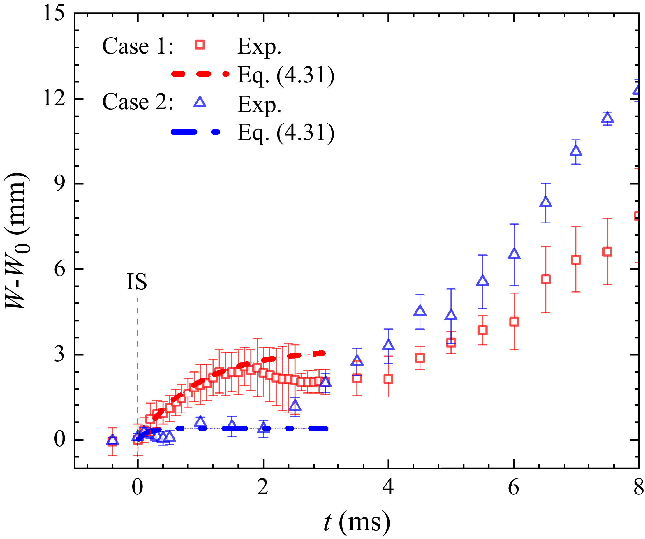
Temporal evolution of the total width of the entire interface reveals the distinct roles of viscosity and elasticity in governing the interfacial dynamics across different cases, as illustrated in figure 3(b). For cases 1 and 2, where viscosity dominates the material behaviour, the interface width (
 $W$
) increases persistently to a maximum value. Subsequently, it gradually decreases due to the restraining effect of elasticity. Notably, case 1 exhibits a higher peak value than case 2, suggesting a comparatively weaker elastic response. Interestingly, during a brief early stage (
 $1.5 \lt t \lt 2.4$
ms), the interface width exhibits a slight decrease, suggesting that elasticity can transiently influence the evolution even in viscosity-dominated systems. For cases 3–5, where elasticity becomes increasingly dominant, the interface width exhibits clear oscillatory behaviour, characterised by a lower growth rate and eventual decay into negative values. Notably, the peak value of
 $W$
decreases systematically with increasing shear modulus from case 3 to case 5. Although the loss factor obtained from rheometer measurements serves as a useful indicator of material dissipation, it does not fully capture the time-dependent strain response under high-rate, transient conditions. The quantitative trends from case 1 to case 5, both in the total width and in the amplitude of the initial small-scale perturbations, reveal a clear transition in interface evolution from viscosity-dominated to elasticity-dominated behaviour. It should also be mentioned that, from case 1 to case 5, both viscosity and shear modulus increase in absolute magnitude, yet their relative dominance shifts, leading to diverse evolution patterns observed in experiment. Note that, due to viscosity, the interface gradually deforms into a 3-D surface along the height direction. Since schlieren imaging provides only an integrated projection along this direction, the resulting overlap makes it difficult to precisely determine the interface position. Therefore, the primary source of experimental uncertainty arises from the 3-D deformation. In addition, the pixel resolution of the camera is approximately 0.17 mm pixel–1, which introduces a baseline measurement error.
4. Theoretical model for gas/viscoelastic RMI
In this section, our theoretical framework employs a scale-decoupled approach, separating the local interfacial dynamics from wall-induced effects. For single-mode perturbation growth, a model is developed based on normal-mode analysis to describe the local interfacial dynamics in the central region, far from the walls. This separation justifies the local application of periodic boundary conditions, under which standard normal-mode analysis and Helmholtz decomposition remain valid. In contrast, a wall-effect model is developed to explicitly account for wall-induced shear deformation by imposing no-slip boundary conditions, thereby capturing viscosity-driven large-scale deformations, such as the V-shaped deformation. The first model focuses on the evolution of initial single-mode perturbations based on potential flow theory, wherein the velocity field is decomposed into irrotational and rotational components following the methodology of Sun, Tao & He (Reference Sun, Tao and He2018). The second model addresses the growth of the V-shaped deformation observed in experiments, considering the interface motion between two parallel plates under no-slip boundary conditions. These two models are applied independently, each addressing distinct physical phenomena at their respective scales.
4.1. Model for single-mode perturbation growth
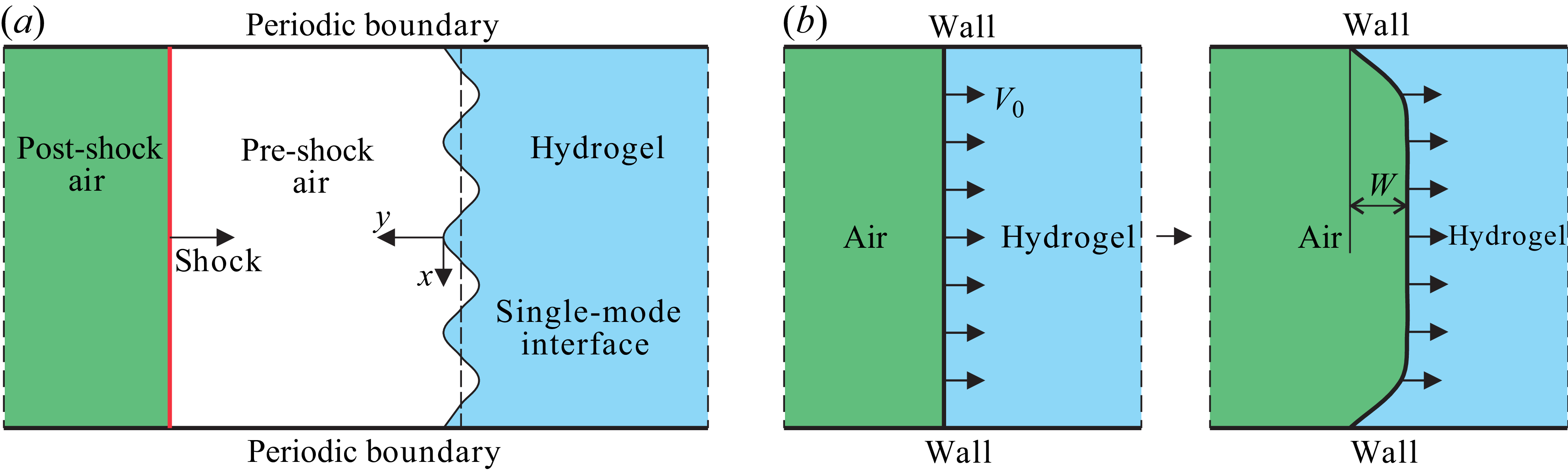
To analyse the evolution of small single-mode perturbations at the gas/hydrogel interface, as depicted in figure 4 (a), we begin with the incompressible 2-D momentum equation
 \begin{equation} \rho _i\frac {\partial U_i}{\partial t}+\rho _i U_i\boldsymbol{\cdot }\boldsymbol{\nabla }U_i=-\boldsymbol{\nabla }P_i+\varPi _i{\nabla} ^2U_i+F_i, \end{equation}
where
 $U_i$
(
 $i=1$
or 2) represents the perturbation velocity of material
 $i$
,
 $P_i$
is the pressure,
 $F_i$
represents external volume forces and
 $\varPi _i$
is a parameter characterising the material’s constitutive properties. Note that
 $F_i$
can be divided into two components: the conservative forces
 $F_{ci}$
and the non-conservative forces
 $F_{nci}$
. For small perturbations, the nonlinear convective term
 $U_i\boldsymbol{\cdot }\boldsymbol{\nabla }U_i$
can be neglected, yielding the linearised equation
 \begin{equation} \rho _i\frac {\partial U_i}{\partial t}=-\boldsymbol{\nabla }P_i+\varPi _i{\nabla} ^2U_i+F_i. \end{equation}
Following the approach of Bellman & Pennington (Reference Bellman and Pennington1954) and Sun et al. (Reference Sun, Tao and He2018), we apply the Helmholtz decomposition to the velocity field, expressing it as the sum of irrotational and rotational components
 $U_i=u_i+v_i$
. This decomposition enables the separation of (4.2) into two distinct parts
 \begin{align} \rho _i \frac {\partial u_i}{\partial t}&=-\boldsymbol{\nabla }P_i + F_{ci} , \end{align}
 \begin{align} \rho _i \frac {\partial v_i}{\partial t}&=\varPi _i\boldsymbol{\nabla} ^2 v_i + F_{nci} . \end{align}
(a) Schematic of the theoretical model. The interface between air and hydrogel is represented by a sinusoidal surface within an infinite plane. Initially, a shock wave travels from left to right, and later hits the air/hydrogel interface, triggering RMI. (b) The air/hydrogel interface starts abruptly between the two plates at velocity
 $V_0$
, subjected to no-slip boundary conditions.

Defining the vorticity as
 $\varOmega _i=\boldsymbol{\nabla }\times v_i$
, we obtain the following evolution equation:
 \begin{equation} \frac {\partial \varOmega _i}{\partial t}=\varPi _i{\nabla} ^2\varOmega _i+\boldsymbol{\nabla }\times F_{nci} . \end{equation}
The solutions to (4.4) and (4.5) can be formulated in terms of potential and streamfunctions
 \begin{align} \phi _i&=A_i e^{\mp ky+nt}\cos {kx}, \end{align}
 \begin{align} \psi _i&=B_i e^{m_iy+nt}\sin {kx}, \\[9pt] \nonumber \end{align}
where
 $k$
is the wavenumber,
 $n$
is the growth rate and
 $m_i$
is determined by the boundary conditions. The irrotational velocity components are given by
 \begin{equation} \left . \begin{aligned} &u_{ix}=\frac {\partial \phi _i}{\partial x}=-kA_ie^{\mp ky+nt}\sin {kx},\\ &u_{iy}=\frac {\partial \phi _i}{\partial y}=\mp k A_ie^{\mp ky+nt}\cos {kx}, \end{aligned} \right \} \end{equation}
while the rotational components are
 \begin{equation} \left . \begin{aligned} &v_{ix}=\frac {\partial \psi _i}{\partial y}=m_iB_ie^{m_iy+nt}\sin {kx},\\ &v_{iy}=-\frac {\partial \psi _i}{\partial x}=-kB_ie^{m_iy+nt}\cos {kx}. \end{aligned} \right \} \end{equation}
Here,
 $A$
and
 $B$
are coefficients to be determined. The total velocity field is given by
 $U_{ix}=u_{ix}+v_{ix}$
and
 $U_{iy}=u_{iy}+v_{iy}$
. The corresponding pressure field is determined from
 \begin{align} P_i&=P_i\vert _{y=y_0}+F_{ci}(y-y_0)+\rho _i\frac {\partial \phi _i}{\partial t}-\rho _i\frac {\partial \phi _i}{\partial t}\vert _{y=y_0}\nonumber\\ &=F_{ci}\int _0^tU_{iy}{\rm d}t+\rho _i\frac {\partial \phi _i}{\partial t}+P_i\vert _{y=y_0}-\rho _i\frac {\partial \phi _i}{\partial t}\vert _{y=y_0}\nonumber\\ &=F_{ci}\frac {U_{iy}}{n}+\rho _i\frac {\partial \phi _i}{\partial t}+C_i, \end{align}
where
 $C_i$
represents an integration constant. For the RMI scenario, we set
 $F=0$
. At the initial condition (
 $t=0$
,
 $y=y_0$
), we have
 $C_1=C_2$
. Across the interface, continuity conditions for both velocity and stress components are required
 \begin{equation} U_{1x}=U_{2x},\quad U_{1y}=U_{2y},\quad S_{1xy}=S_{2xy},\quad S_{1yy}=S_{2yy}, \end{equation}
where the stress components are
 \begin{align} S_{ixy}&=\varPi _i\left (\frac {\partial U_{iy}}{\partial x}+\frac {\partial U_{ix}}{\partial y}\right )+T_{ixy}, \end{align}
 \begin{align} S_{iyy}&=-P_i+2\varPi _i\frac {\partial U_{iy}}{\partial y}+T_{iyy}. \end{align}
Here,
 $T$
is the stress tensor caused by the non-conservative force
 $F_{nc}$
. By applying these boundary conditions and also performing algebraic simplifications, we derive the following system of equations:
 \begin{equation} \left \{ \begin{aligned} -kA_1+m_1B_1+kA_2-m_2B_2 &= 0,\\ A_1+B_1-A_2+B_2 &= 0,\\ \varPi _1(k^2A_1+k^2B_1+k^2A_1+m_1^2B_1) &= \varPi _2(k^2A_2+k^2B_2+k^2A_2+m_2^2B_2),\\ -\rho _1n+2\varPi _1(k^2A_1-km_1B_1) &= -\rho _2n+2\varPi _2(k^2A_2-km_2B_2). \end{aligned} \right . \end{equation}
Solving this system of equations analytically yields the dispersion relation for the growth rate
 $n$
 \begin{equation} n\left [\frac {1}{\varPi _1+\varPi _2\sqrt {1+\frac {\rho _2n}{\varPi _2k^2}}}+\frac {1}{\varPi _2+\varPi _1\sqrt {1+\frac {\rho _1n}{\varPi _1k^2}}}\right ]+\frac {4k^2}{\rho _1+\rho _2}=0. \end{equation}
When considering the friction between the hydrogel block and acrylic box (
 $F_{c}=f$
, the frictional force
 $f$
in one direction can be considered as a conservative force
 $F_{nc}$
), the dispersion relation becomes
 \begin{equation} \left (n+\frac {fk}{n}\right )\left (\frac {1}{\varPi _1+\varPi _2\sqrt {1+\frac {\rho _2 n}{\varPi _2 k^2}}}+\frac {1}{\varPi _2+\varPi _1\sqrt {1+\frac {\rho _1 n}{\varPi _1 k^2}}}\right )+\frac {4k^2}{\rho _1+\rho _2}=0, \end{equation}
with the additional assumption that
 $\dot {\rho }/\rho = \dot {\rho }_2/\rho _2 \approx \dot {\rho }_1/\rho _1$
. Assuming the initial conditions
 $U_{1y}|_{t=0}=U_{2y}|_{t=0}=v_0$
, where
 $v_0$
is the post-shock interface velocity, we derive expressions for the velocity components
 $U_{ix}$
and
 $U_{iy}$
. Neglecting nonlinear terms, the interface evolution equation
 $y=\eta (x,t)$
simplifies to
 \begin{equation} \eta = \int U_{iy} dt = \frac {k(\mp A_i e^{\mp ky} - B_i e^{m_iy})}{n} e^{nt} \cos kx. \end{equation}
To complete the model, it is necessary to specify the constitutive relations for the viscoelastic material. We consider two limiting cases. For a Hookean elastic solid, the stress tensor
 $\tau _{ij}$
obeys the relationship
 \begin{equation} \frac {\partial \tau _{ij}}{\partial t}=G\left (\frac {\partial U_i}{\partial x_{\!j}}+\frac {\partial U_{\!j}}{\partial x_i}\right ), \end{equation}
where
 $G$
is the shear modulus. For a viscous fluid, the stress tensor is given by
 \begin{equation} \tau _{ij}=\mu \left (\frac {\partial U_i}{\partial x_{\!j}}+\frac {\partial U_{\!j}}{\partial x_i}\right ), \end{equation}
where
 $\mu$
is the dynamic viscosity. To model viscoelastic materials, which exhibit both viscous and elastic characteristics, we adopt the Maxwell model. This model represents the material as an ideal viscous dashpot and an ideal elastic spring arranged in series. The corresponding stress–strain relationship is given by
 \begin{equation} \tau +\frac {\mu }{G}\dot {\tau }=\mu \dot {\varepsilon }. \end{equation}
During the initial growth phase, when perturbations grow as
 $e^{nt}$
, we have
 $\tau _{ij}=\frac {1}{n}\frac {\partial \tau _{ij}}{\partial t}$
. Substituting this into the Maxwell model yields
 \begin{equation} \tau _{ij}=\frac {1}{\dfrac {1}{\mu }+\dfrac {n}{G}}\left (\dfrac {\partial U_i}{\partial x_{\!j}}+\dfrac {\partial U_{\!j}}{\partial x_i}\right )\!. \end{equation}
Therefore, the material parameter
 $\varPi$
in our model is
 \begin{equation} \varPi =\frac {1}{\dfrac {1}{\mu }+\dfrac {n}{G}}. \end{equation}
By substituting the expression of
 $\varPi$
into the dispersion relation (4.16), we obtain the following equation governing the growth rate:
 \begin{align} \left (n+\frac {fk}{n}\right )\left (\frac {1}{\frac {1}{\frac {1}{\mu _1}+\frac {n}{G_1}}+\frac {1}{\frac {1}{\mu _2}+\frac {n}{G_2}}\sqrt {1+\frac {\rho _2 n}{\frac {1}{\frac {1}{\mu _2}+\frac {n}{G_2}} k^2}}}+\frac {1}{\frac {1}{\frac {1}{\mu _2}+\frac {n}{G_2}}+\frac {1}{\frac {1}{\mu _1}+\frac {n}{G_1}}\sqrt {1+\frac {\rho _1 n}{\frac {1}{\frac {1}{\mu _1}+\frac {n}{G_1}} k^2}}}\right ) \notag \\+\frac {4k^2}{\rho _1+\rho _2}=0, \end{align}
where
 $\mu _1$
and
 $G_1$
represent the dynamic viscosity and shear modulus of air, while
 $\mu _2$
and
 $G_2$
denote the corresponding properties for the gel. When combined with (4.17), the evolution of the initial single-mode perturbation at the interface can be obtained.
4.2. Model for V-shaped perturbation growth
To theoretically analyse the V-shaped perturbation growth, we focus on the post-shock behaviour of the hydrogel. Note that given the hydrogel block’s small height (6 mm) relative to its width (120 mm) and length (115 mm), the vertical deformations (3-D effects) are considered secondary effects and are excluded from the present analysis. This simplification is justified by the predominantly 2-D nature of the flow field under these geometric constraints. Here, we approximate it as a 2-D fluid confined between two infinitely large parallel plates, as depicted in figure 4(b). The fluid is suddenly set into motion with an initial velocity
 $V_0=u_0$
within its own plane, subject to no-slip boundary conditions.
The interface velocity
 $V(x,t)$
is governed by the following equation:
 \begin{equation} \frac {\partial V}{\partial t}=\nu \frac {\partial ^2 V}{\partial x^2}, \end{equation}
where
 $\nu$
represents the kinematic viscosity. No-slip boundary conditions are applied at the plates:
 $V(0,t)=V(l,t)=0$
, where
 $l$
denotes the height of the interface in the
 $x$
direction. Using the method of separation of variables, we assume a solution of the form
 $V(x,t) = Y(x)T(t)$
, which leads to the following equation:
 \begin{equation} \frac {Y''(x)}{Y(x)} = \frac {T'(t)}{\nu T(t)} = -\lambda . \end{equation}
This separation produces two ordinary differential equations. For the spatial function
 $Y(x)$
, we have
 \begin{align} Y''(x) + \lambda Y(x) &= 0, \end{align}
 \begin{align} Y(0) = Y(l) &= 0, \end{align}
and for the temporal component
 $T(t)$
, we have
 \begin{equation} T'(t) + \lambda \nu T(t) = 0. \end{equation}
The general solution for the velocity profile is then given by
 \begin{equation} V(x,t) = \sum _{n=0}^\infty C_n \exp \left (-\frac {n^2 \pi ^2 \nu }{l^2} t \right ) \sin \left (\frac {(n+\frac {1}{2})\pi }{l} x \right )\!. \end{equation}
To determine the coefficients
 $C_n$
, we use the initial velocity condition:
 $V(x,0) = u_0$
for
 $0 \lt x \lt l$
, where
 $u_0$
is the post-shock interface velocity
 \begin{equation} C_n = \frac {2}{l} \int _0^l V(x,0) \sin \left (\frac {n\pi }{l} x\right ) \, {\rm d}x. \end{equation}
This yields the complete solution for the velocity profile
 \begin{equation} V(x,t) = \sum _{n=0}^\infty C_n \exp \left (-\frac {n^2 \pi ^2 \nu }{l^2} t\right ) \sin \left (\frac {(n+\frac {1}{2})\pi }{l} x\right )\!. \end{equation}
Finally, the total width of the long-wavelength (V-shaped) perturbation
 $W$
can then be obtained by integrating the velocity field
 \begin{equation} W(t) = \int V(x=\frac {l}{2},t) \, {\rm d}t-\int V(x=l,t) \, {\rm d}t=\int V(x=\frac {l}{2},t) \, {\rm d}t \end{equation}.
5. Model validation against experiment
In the early stages, nonlinearity is negligible and the small perturbation amplitude grows almost linearly with time. For gas/gas interfaces, the linear growth rate can be estimated using the impulsive model
 \begin{equation} \dot {a}=kA\Delta V a_0. \end{equation}
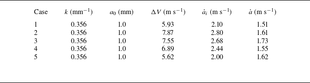
Table 2 shows that the experimental growth rates are consistently lower than the theoretical predictions from the impulsive model. This systematic discrepancy can be attributed to the complex mechanical response of the hydrogel block under shock loading. Specifically, upon impact, the hydrogel undergoes significant compression, generating a multi-directional stress field that propagates outward from the interface. This corresponds to the generation of shear waves in the hydrogel block (seen in figure 2), which transports energy away from the interface, acting as a dissipative mechanism.
The growth rates of single-mode perturbation for various cases. Here,
 $\Delta V$
is the jump velocity of the interface subjected to shock,
 $\dot {a}_i$
is growth rate calculated using the impulsive model and
 $\dot {a}$
is the measured one in experiments.

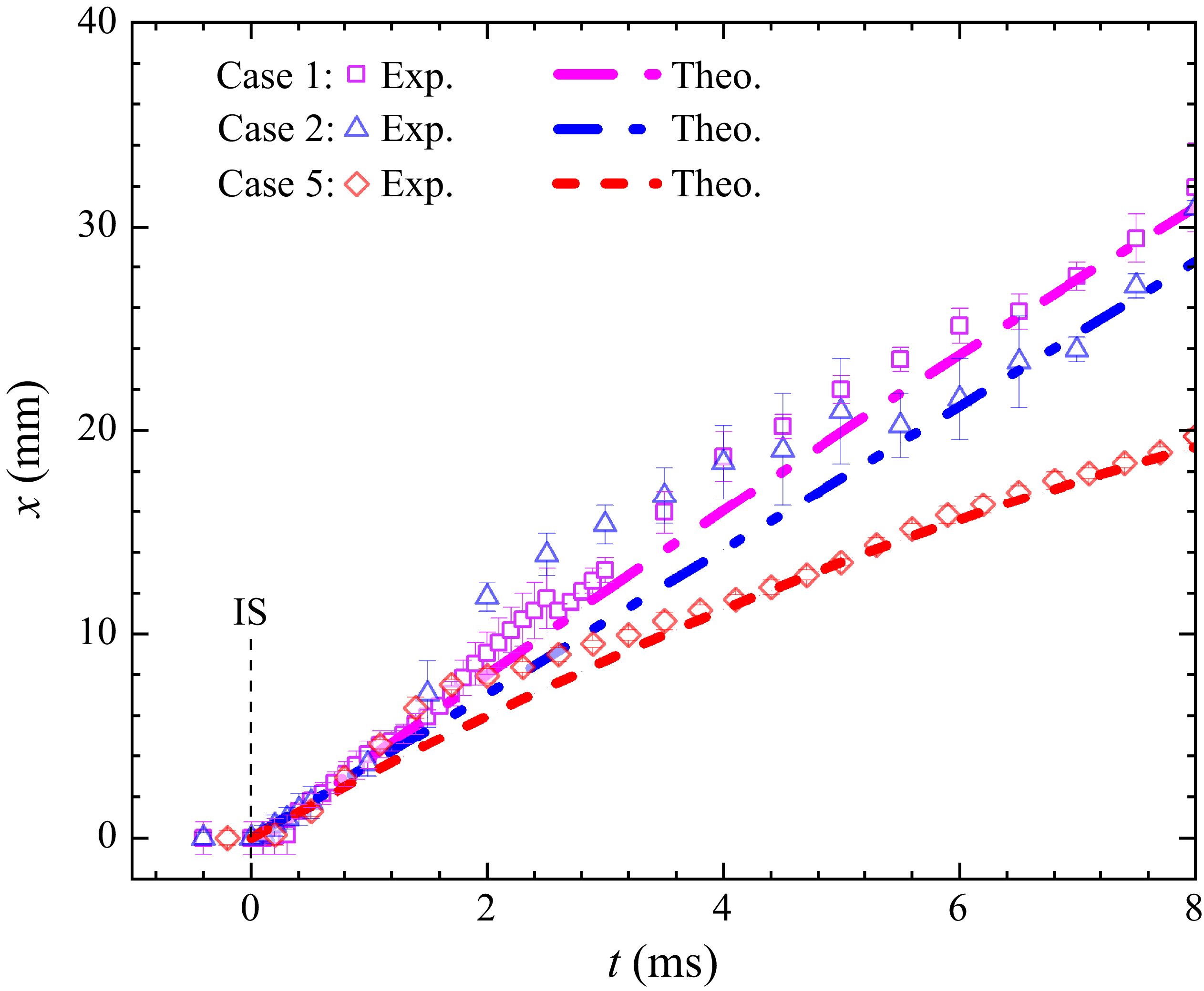
Displacement of the block’s left boundary, showing good agreement with the uniform deceleration model when an appropriate frictional force is applied. Here, IS indicates the incident shock.

The frictional forces exerted by the acrylic container on the hydrogel dominate the block’s motion, allowing its global motion to be approximated as uniformly decelerated. We estimate the effective frictional force by comparing the measured block displacement with the analytical solution for uniformly decelerated motion, iteratively adjusting the friction term until agreement is achieved. Incorporating the calculated friction forces, the uniform deceleration model gives reasonable predictions of the displacement of the block’s left boundary, as shown in figure 5. This approach provides a practical method to estimate the magnitude of the frictional force acting on the hydrogel block, which is a critical parameter subsequently incorporated into equation (4.23). It is generally found that under our experimental conditions, the resulting force is very small (
 $\lt$
10 N), such that its influence on interface evolution can be neglected. Figure 6(a) shows the time-dependent strain rate of the hydrogel for cases 3 and 5, where the shear rate is roughly estimated by the rate of change in single-mode perturbation amplitude. Immediately after shock impact, the interfacial strain rate reaches a peak and then gradually decreases with visible oscillations for each case. This behaviour underscores the importance of accounting for strain-rate effects on the hydrogel’s properties. As illustrated in figure 6(b), for all cases considered in this work, the shear modulus varies significantly with increasing the shear rate. It indicates that the strain-rate-dependent properties of the hydrogel are important for accurately predicting the RMI behaviour.
(a) Temporal evolution of strain rates under different experimental conditions; (b) shear modulus of various materials as a function of strain rate.

(a) Comparison of the single-mode perturbation growth for the viscous case with the prediction of (4.23); (b) comparison of the single-mode perturbation growth for the elastic case with the prediction of (4.23); (c) comparison of the single-mode perturbation growth for case 4 with (4.23) and its simplified version that neglects viscosity.

Figures 7(a) and 7(b) compare the evolution of single-mode perturbation amplitudes between experiments and predictions based on (4.23) for both viscosity-dominated and viscoelastic-dominated cases. As shown in table 1, rheological measurements for case 5 reveal a pronounced strain-rate dependence of the hydrogel’s shear modulus, increasing from 21 478 Pa at 10 rad s−1 to 65 130 Pa at 100 rad s−1. Considering this strain-rate dependence, different modulus values are adopted in the model to reflect the strain-rate variations: 65 130 Pa is applied during the early stage when strain rates reach up to 255 rad s−1, whereas 21 478 Pa is used in the later oscillatory phase, where strain rates range from 0 to 116 rad s−1, as shown in figure 6. For the intermediate regime where strain rates remain below 100 rad s−1, the model adopts material properties measured at 10 rad s−1 as a compromise. This simplified approach, relying on discrete shear modulus values, successfully captures the oscillatory behaviour of single-mode perturbations across all cases. However, it consistently underestimates the oscillation periods compared with experimental results. This discrepancy likely arises from the limitations of approximating continuously varying strain-rate behaviour using discrete material parameters. In addition, the shear-thickening behaviour of the material (e.g. strain-rate-dependent modulus) and viscosity, are not considered in the model. A deviation between the experimental and theoretical results for cases 1 and 2 is observed at later stages, which can also be attributed to plastic deformation. For viscoelastic materials, a precise theoretical prediction of the elastic deformation limit is not currently available. Following Piriz, López Cela & Tahir (Reference Piriz, López Cela and Tahir2008), for purely elastic materials, the amplitude
 $a_p$
at the elastic limit can be estimated as:
 $a_p-a_0=\sqrt {({2}/{3})}({1}/{2\vert M \vert })({Y}/{\textit{kG}})$
, where
 $Y$
is the yield strength, and
 $\vert M \vert$
is an empirical coefficient obtained from numerical calculations (
 $\vert M \vert = 0.91$
in elastic regime). According to this estimation, the elastic limits for the cases 1–5 are 1.6, 1.5, 1.6, 2.0 and 1.7 mm, respectively. These results indicate that plastic deformation takes place in cases 1 and 2, while cases 4 and 5 remain within the elastic regime. To further analyse the effects of elasticity and viscosity, the model is evaluated with viscosity set to zero. The results are compared with both experimental data and calculations using the full model with non-zero viscosity, as shown in figure 7(c). When viscosity is neglected, the amplitude shows almost no decay. The present analysis demonstrates that elasticity governs the oscillation period of the amplitude, while viscosity has minimal influence on the period but significantly contributes to amplitude attenuation.
Comparisons between experiments and model predictions for the V-shaped perturbation growth in viscosity-dominated cases. Error bars represent measurement uncertainties arising from the finite thickness of the interface.

Figure 8 presents a comparison of the temporal evolution of the total width of the V-shaped interface between the experiments and the model predictions based on (4.32) for cases 1 and 2. In the early stages, the experimental results exhibit good agreement with the theoretical predictions. However, the model predicts an earlier saturation of amplitude growth compared with the experimental data. This discrepancy can be attributed to several factors. First, the viscosity coefficient employed in the theoretical model may overestimate the actual value, especially under dynamic loading conditions. Second, the model neglects elasticity effects. Additionally, the hydrogel’s actual deformation field is three-dimensional, involving coupled lateral and longitudinal components that introduce mechanical responses not captured by the current 2-D theoretical framework.
The quantitative comparison between experiment and theory highlights both the strengths and the limitations of the model developed in this work. The model reproduces the amplitude oscillations reasonably well in elasticity-dominated cases, but significant discrepancies appear in viscosity-dominated cases, indicating that rate-dependent, dissipative mechanisms are not fully captured. A major simplification of our model is the incompressible-flow assumption: compressibility and EoS effects are crucial for RMI, especially in the early-time, pressure-wave-dominated regime. Previous studies have demonstrated that models developed under the incompressible-flow assumption (Richtmyer Reference Richtmyer1960; Meyer & Blewett Reference Meyer and Blewett1972; Vandenboomgaerde, Rouzier & Souffland Reference Vandenboomgaerde, Rouzier and Souffland2018) are generally accurate only for weak shocks or low-compressibility conditions. To establish a more reliable model applicable under various shock strengths, the exact linear problem must be solved (Napieralski et al. Reference Napieralski, Cobos and Velikovich2024). Also, as noted by Ward & Pullin (Reference Ward and Pullin2011), RMI development exhibits distinct features when comparing fluids obeying the perfect-gas EoS with those described by the non-ideal Mie–Grüneisen EoS, commonly used for solids and liquids. In the latter case, the much higher sound speed leads to faster perturbation propagation and response, and consequently, the growth-rate oscillation presents higher frequency and larger amplitude. Despite these, the current model’s applicability is primarily justified by two experimental conditions: (i) the post-start-up phase, where the flow approaches an incompressible state when the shock waves have moved away from the interface, as noted by Zhang et al. (Reference Zhang, Deng and Guo2018); and (ii) the relatively low shock Mach number (
 $Ma = 1.29 \pm 0.04$
) in our study, which limits compressibility effects compared with high-Mach-number scenarios. These factors explain the good agreement observed for post-start-up interface evolution, while also accounting for the model’s limitations at early times and in viscosity-dominated regimes. Future extensions will incorporate compressibility corrections, more realistic EoS and improved treatment of rate-dependent viscous responses, which should enhance predictive accuracy for early-time dynamics and higher-Mach regimes.
6. Conclusions
In this study, we systematically investigate the RMI at single-mode gas/hydrogel interfaces through shock tube experiments and theoretical analysis. By developing a novel experimental platform utilising hydrogels with tuneable viscoelastic properties, we revealed several key findings. First, we demonstrate that the growth of viscoelastic RMI is fundamentally determined by the material’s loss factor, which characterises the relative dominance of viscous and elastic effects. For materials with high loss factors, the interface evolution follows a characteristic viscosity-dominated pattern featuring V-shaped deformation and gradual attenuation of the single-mode perturbation. In contrast, materials with low loss factors exhibit distinct elastic-dominated behaviour, characterised by sustained oscillations of initial single-mode perturbations with reduced amplitudes. Second, we establish a theoretical framework based on linear stability analysis that incorporates both viscous and elastic effects through the Maxwell model. This model successfully captures the essential physics of viscoelastic RMI, particularly the transition from viscous to elastic dominated regimes. The model accurately predicts the growth of single-mode perturbation in viscoelastic-dominated cases and the oscillatory behaviour in elastic-dominated cases. However, quantitative deviations emerge at later times. Our experimental measurements reveal significant strain-rate dependence of the hydrogel’s mechanical properties, with shear modulus varying by up to 300 % across different loading rates. This strain-rate sensitivity, combined with potential microstructural evolution, contributes to the observed discrepancies between theoretical predictions and experimental results, particularly in the oscillation periods and late-time amplitude growth.
This study establishes RMI experiments as a promising technique for characterising viscoelastic material behaviour under dynamic loading conditions. The rich interfacial dynamics observed provides unique insights into material response that complement conventional rheological measurements. Our findings lay the groundwork for developing more accurate models for the evolution of viscoelastic materials under shock loading conditions.
Supplementary movies
Supplementary movies are available at https://doi.org/10.1017/jfm.2025.10954.
Acknowledgements
The authors gratefully acknowledge Professor Y. Sun for his valuable suggestions.
Funding
This work was supported by the National Natural Science Foundation of China (nos. 12388101, 12532013), the Science Challenge Projects (TZ2025016), the Strategic Priority Research Program of Chinese Academy of Science (XDB1100120, XDB0500301) and the National Key Research and Development Program of China (2022YFF0504500).
Declaration of interests
The authors report no conflict of interest.