1. Introduction
Turbulent boundary layers (TBLs) have been the focus of pioneering research since the nineteenth century. The technological advances in experimental techniques have played a major role in providing a deeper understanding of the characteristics of TBL. Some key aspects of open channel flows have been borrowed from classical TBLs due to the strong resemblance of the flow physics (Keulegan Reference Keulegan1938; Roussinova, Biswas & Balachandar Reference Roussinova, Biswas and Balachandar2008). Similar to a classical TBL, the near-wall boundary layer like zone in open channel flow is divided into four distinct regions: the viscous sublayer, buffer layer, logarithmic layer and defect layer. Taken together, the first three layers up to and including the logarithmic layer are called the inner layer and the outer layer is a combination of the logarithmic and defect layers. Therefore, the logarithmic layer is also known as the overlapping region between the inner and outer regions of the boundary layer. The flow velocities in the viscous sublayer can be predicted as  $U/{U_\tau } = y{U_\tau }/\upsilon $ (U is the mean streamwise velocity,
 ${U_\tau }$ is the wall-shear velocity, y is wall-normal coordinate,
 $\upsilon $ is kinematic viscosity) whereas the flow velocity in the overlap region is estimated by the ‘log law’ proposed by Clauser (Reference Clauser1956)
 \begin{equation}\begin{array}{*{20}{c}} {\dfrac{U}{{{U_\tau }}} = \dfrac{1}{\kappa }\ln \left( {\dfrac{{y{U_\tau }}}{\upsilon }} \right) + B} \end{array},\end{equation}
where y is distance from the wall and, for a smooth wall, the von Kármán constant  $\kappa $ varies in the range 0.39 to 0.42, and B is a constant between 5.0 and 5.5 (Steffler, Rajaratnam & Peterson Reference Steffler, Rajaratnam and Peterson1985; Nezu & Rodi Reference Nezu and Rodi1986; Kirkgöz & Ardiçlioğlu Reference Kirkgöz and Ardiçlioğlu1997; Balachandar & Ramachandran Reference Balachandar and Ramachandran1999; Balachandar et al. Reference Balachandar, Blakely, Tachie and Putz2001; Roussinova et al. Reference Roussinova, Biswas and Balachandar2008; Heidari et al. Reference Heidari, Balachandar, Roussinova and Barron2017; Miguntanna et al. Reference Miguntanna, Moses, Sivakumar, Yang, Enever and Riaz2020). A validation of the logarithmic law has been rigorously used by researchers as a measure to confirm a standardized flow behaviour. Since the log law is incapable of predicting the velocity distribution in the defect layer, Coles (Reference Coles1956) proposed a ‘velocity defect law’ where a wake function w is introduced to incorporate the deviation of the defect layer velocity data from the log law. This modified log law can be expressed in the form of ‘mean velocity deficit’ as a function of y/δ,
 \begin{equation}\begin{array}{*{20}{c}} {\dfrac{{{U_\infty } - U}}{{{U_\tau }}} = f(y/\delta ) ={-} \dfrac{1}{\kappa }\ln \left[ {\; \dfrac{y}{\delta }\; } \right] + \; \dfrac{{2\varPi }}{\kappa }\left[ {w\left( {\dfrac{y}{\delta }} \right)} \right],} \end{array}\end{equation}
where  $\delta $ is the boundary layer thickness and
 $\varPi$ is the wake parameter. However, there is no consensus among researchers on the nature of the wake function and the value of
 $\varPi$ as applied to both TBL and open channel flow. Chauhan, Monkewitz & Nagib (Reference Chauhan, Monkewitz and Nagib2009) proposed a modified defect law, referred to as the ‘velocity composite law’ where the wake function is derived by fitting a curve to the experimental data. It should also be noted that the above equations, although adopted in open channel flow, were initially developed for a canonical zero-pressure-gradient TBL.
The state of flow in a typical test section is mostly governed by two parameters, the flow development length and the nature of the upstream tripping to enhance the growth of the boundary layer. These two parameters can be finely adjusted to stimulate a well-behaved TBL. Erm & Joubert (Reference Erm and Joubert1991) varied the type of tripping using wire, distributed grit and cylindrical pins to match  $\varPi$ with that of a standard boundary layer. Marusic et al. (Reference Marusic, Chauhan, Kulandaivelu and Hutchins2015) showed that the flow characteristics at the same Reynolds number may differ if the tripping pattern and the flow development length are varied. On the other hand, Monkewitz, Chauhan & Nagib (Reference Monkewitz, Chauhan and Nagib2007) and Chauhan, Nagib & Monkewitz (Reference Chauhan, Nagib and Monkewitz2007) reported that there should be a state of equilibrium in zero-pressure-gradient (ZPG) TBLs where
 $\varPi$ becomes invariant. Therefore, any ZPG boundary layer flow with a trip can be divided into two regions in the streamwise span: (i) the development regime and (ii) the well-behaved flow regime. The flow development regime is the region immediately downstream of the trip where the turbulence generated by the roughness element can cause a different flow behaviour than what is expected in a boundary layer flow. This turbulence gets distributed and adequately dissipated to reach a well-behaved canonical state further downstream. As a matter of fact, a similarity in Reynolds number is a mandatory but not a sufficient criterion to compare two TBL flows since their turbulence distribution can be significantly different based on the tripping intensity and flow development length. In addition, the effect of the free surface plays a crucial role when the near-wall flow in an open channel is considered for analysis. Importantly, the effects of tripping and the free surface are often neglected in open channel flow studies and a proper guideline on this matter has not been set.
Tripping is widely used in open channel flumes to quicken the change of an initially laminar boundary layer to a turbulent state, and to achieve a fully developed state with a short flow development length. An open channel flow is termed fully developed if there is no streamwise variation of the flow variables. This is only possible when the boundary layer thickness is constant along the streamwise span of the flume, otherwise wall-normal distributions of the flow variables will vary between different streamwise positions. The primary method of generating a fully developed open channel flow is by allowing the flow to develop gradually from the inlet section of a flume until the boundary layer thickness is equal to the flow depth. Since this procedure requires a very long flow development length, in most laboratory flumes a fully developed state cannot be generated without inflow tripping. But tripping does not necessarily ensure a fully developed state in open channel flow as it can only reduce the required flow development length to a certain extent. The size and the roughness height of the trip can be optimally adjusted to ensure a fully developed flow in the measurement section, provided an adequate flow development length corresponding to the flow depth and the Reynolds number is available. With a lower level of tripping (referred to here as an under-tripped case) the flow can still be in a developing state at the measurement location. On the other hand, if the intensity of perturbations generated from the trip is very high (i.e. over-tripped case), it may take a longer distance to dissipate the additional energy before reaching a well-behaved canonical state. Therefore, if the other hydraulic parameters are held constant, to ensure a fully developed state, there should be one suitable trip condition (a narrow range of roughness height for the trip or the tripping intensity) for which the boundary layer thickness will be equal to the flow depth and simultaneously retain the canonical behaviour.
To identify if the flow has become fully developed, the simplest approach is to carry out measurements at several streamwise positions and study the variation in the profiles of velocity or other flow variables, but this approach is very tedious. It has become a common practice to use the validation of the logarithmic or defect law to ensure canonical behaviour. But this method can only confirm a well-behaved boundary layer, not a fully developed state. The fully developed flow is the state for which the boundary layer thickness is the same as flow depth, while retaining the properties of a standard boundary layer. Therefore, another widely used approach is to determine the boundary layer thickness accurately at the test location. The conventional way of estimating boundary layer thickness is to find the bed-normal coordinate at which streamwise velocity is  $0.99{U_\infty }$. This approach works reasonably well when there is a clear and undisturbed free-stream region. Since the turbulence intensity is negligible in the free-stream region and the velocity is fairly constant, it is possible to accurately determine δ and
 ${U_\infty }$ in a zero-pressure-gradient TBL. Hearst et al. (Reference Hearst, de Silva, Dogan and Ganapathisubramani2021) noticed issues with this approach and determined the boundary layer thickness using the streamwise Reynolds normal stress profile. In open channel flow,
 ${U_\infty }$ is commonly taken as the maximum velocity near the free surface. As a matter of fact, the estimation of boundary layer thickness in open channel flows is highly influenced by secondary currents, free surface perturbations and confinement of the upward momentum transfer, thus causing disparity among the experimental studies. The difficulty is compounded for the case of the fully developed open channel flow where no free-stream region is present. It is perhaps technically more suitable to quantify the boundary layer thickness using the wall-normal distribution of Reynolds stresses and higher-order moments which are directly related to the depth-wise variation of turbulence generation, intermittency, ejection and sweep events (Andreopoulos et al. Reference Andreopoulos, Durst, Zaric and Jovanovic1984; Gad-el Hak & Bandyopadhyay Reference Gad-el Hak and Bandyopadhyay1994; Balachandar & Patel Reference Balachandar and Patel2005; Balachandar & Bhuiyan Reference Balachandar and Bhuiyan2007). The boundary layer thickness can be more precisely defined as the wall-normal position above which Reynolds stresses and higher-order moments become nominally constant and this definition is consistent with previous studies (Flack, Schultz & Shapiro Reference Flack, Schultz and Shapiro2005; Roussinova et al. Reference Roussinova, Biswas and Balachandar2008). Using this approach will enable us to consistently define a fully developed state in open channel flow.
The wall-bounded flow in an open channel is found to differ from that of a classical TBL due to the existence of the free surface which behaves like a weak wall and can have a significant impact on the flow properties (Nezu Reference Nezu2005). The large-scale and very-large-scale fluid motion in open channel flow can also be different from that noticed in a well-behaved TBL and the free surface can have an impact on the inner flow properties by sustaining or promoting the formation of large-scale fluid motions (Duan et al. Reference Duan, Chen, Li and Zhong2020; Peruzzi et al. Reference Peruzzi, Poggi, Ridolfi and Manes2020). These dissimilarities can be seen prominently in the instantaneous flow characteristics if the boundary layer thickness is very close to the free surface such as that in the fully developed state. As mentioned earlier, an adequate tripping and an accurate estimate of boundary thickness can be used to generate a fully developed state based on the time-averaged characteristics of open channel flows. Once the depth-wise variation of time-averaged variables is consistent with the flow physics of a fully developed state, the instantaneous flow properties can be explored further to study the effect of the free surface.
The deviation in flow characteristics of a fully developed open channel flow from that of a developing flow or a classical TBL flow is mostly caused by the vertical confinement due to the free surface. As momentum transfer near the free surface is restricted in the vertical direction, it has to be transferred through the surrounding fluid to the other directions. A momentum zone analysis will be useful to gain insights into these attributes of the flow field. Momentum zone analysis has been previously carried out in ZPG TBLs (Adrian, Meinhart & Tomkins Reference Adrian, Meinhart and Tomkins2000; de Silva, Marusic & Hutchins Reference de Silva, Marusic and Hutchins2014; Eisma et al. Reference Eisma, Westerweel, Ooms and Elsinga2015; de Silva et al. Reference de Silva, Philip, Hutchins and Marusic2017; Laskari et al. Reference Laskari, de Kat, Hearst and Ganapathisubramani2018; Heisel et al. Reference Heisel, De Silva, Hutchins, Marusic and Guala2020) and in pipe flows (Chen, Chung & Wan Reference Chen, Chung and Wan2020), which has enhanced our understanding of large-scale motions. Meinhart & Adrian (Reference Meinhart and Adrian1995) observed layers of uniform momentum in TBLs. Each of the momentum zones corresponds to a ‘modal velocity’ and can be identified by the local peaks in the probability density function of streamwise velocity (Adrian et al. Reference Adrian, Meinhart and Tomkins2000). Chauhan et al. (Reference Chauhan, Philip, de Silva, Hutchins and Marusic2014b) proposed a method to differentiate between the rotational and irrotational regions, and the interface between these regions is commonly known as the turbulent/non-turbulent interface (TNTI). Uniform momentum zones lie inside the TNTI and Eisma et al. (Reference Eisma, Westerweel, Ooms and Elsinga2015) pointed out the co-existence of these momentum zones in the region between the bed and the TNTI. The momentum zones have been used to depict the flow characteristics by relating the number of momentum zones with the flow Reynolds number (de Silva, Hutchins & Marusic Reference de Silva, Hutchins and Marusic2016). The number of zones increases log–linearly with the increase of Reynolds number and the thickness of these zones increases away from the bottom wall. Laskari et al. (Reference Laskari, de Kat, Hearst and Ganapathisubramani2018) extended the analysis to the time evolution of the momentum zones. They observed large-scale quadrant 2 (Q2) events when the number of momentum zones is large and quadrant 4 (Q4) events with a smaller number of momentum zones. The Q2 and Q4 events correspond to ejections and sweeps, respectively, and thus create a coherence of large-scale fluid motions associated with the momentum zones. In this paper, the main purpose of the momentum zone analysis is to illustrate why adequate tripping is mandatory to achieve a fully developed flow and how the flow properties may vary when the flow is not truly fully developed.
Maintaining a fully developed state for the flow approaching the test section is an important consideration to achieve repeatability in flow behaviour and to directly compare results from different experimental facilities. If the approach flow is in a developing state, the vertical distribution of the mean and turbulence quantities will vary in the streamwise direction and be different from set-up to set-up. Therefore, the primary focus of the current research is to present a rational methodology for stimulating a fully developed open channel flow by varying the inflow tripping. The bed-normal distributions of mean velocity, Reynolds stresses and higher-order moments of the test cases corresponding to different trips are compared in this context. The self-similarity of the fully developed flow is also validated using results from the literature. The second objective of this paper is to investigate the differences in flow properties of a developing and a developed flow in an open channel which indirectly depicts the effects of tripping and the free surface. The variation in quadrant events between the developing and fully developed cases is identified using conditional averaging of the instantaneous flow variables corresponding to the different number of momentum zones and large-scale fluid motions.
2. Experiment set-up and test conditions
The present experiments were carried out in a recirculating open channel flume at the Hydraulic Engineering Research Laboratory at the University of Windsor. A schematic diagram of the flume is presented in figure 1. The flume has a rectangular cross-section with a length of 16 m, a width (b) of 1.2 m and a height of 0.8 m. The sides and bottom walls of the flume are made of transparent glass to provide optical access to the flow. The upstream settling tank ensures reduction of inflow perturbations and honeycomb flow straighteners are also used to manage the turbulence level. The tailgate at the downstream end of the flume controls the water depth. Since a clear free-stream region is not present in a fully developed open channel flow,  ${U_\infty }$ is commonly taken as the maximum velocity near the free surface. The flow characteristics were studied using two aspect ratios, b/H = 9 (H = 0.135 m) and 7 (H = 0.170 m) at a constant Reynolds number
 $(R{e_H})$ of 39 000 based on flow depth H and free-stream velocity
 ${U_\infty }$. These aspect ratios are high enough (>5) to minimize the effect of secondary flows (Nakagawa & Nezu Reference Nakagawa and Nezu1977; Nezu & Rodi Reference Nezu and Rodi1986; Yang, Tan & Lim Reference Yang, Tan and Lim2004; Bonakdari et al. Reference Bonakdari, Larrarte, Lassabatere and Joannis2008; Mahananda et al. Reference Mahananda, Hanmaiahgari, Ojha and Balachandar2019). For these aspect ratios, a section of the flow in the central region of the channel can be considered to be nominally two-dimensional (Nasif, Balachandar & Barron Reference Nasif, Balachandar and Barron2020). In this case there is no measurable spanwise variation in mean streamwise velocity profile over the mid 80 % of the flume width and the ratio of mean spanwise velocity to mean streamwise velocity is less than ±0.005. Over a streamwise length of 5 m, the change in water depth is approximately 0.5 mm, corresponding to a pressure-gradient parameter (β) of −1.3 in the low aspect ratio tests and −2.1 in the higher aspect ratio tests. These values for β indicate that the flow is mildly accelerating (Peruzzi et al. Reference Peruzzi, Poggi, Ridolfi and Manes2020). However, as suggested by Kironoto & Graf (Reference Kironoto and Graf1995), Song & Chiew (Reference Song and Chiew2001) and Pu et al. (Reference Pu, Tait, Guo, Huang and Hanmaiahgari2018), the effect of non-uniformity can be considered as negligible for the present values of β.
Schematic of the recirculating flume and test set-up.

The tests were conducted on a smooth bed with and without trips to generate the desired flow conditions. A primary trip (T1) made of a patch of coarse grain sand particles ( ${k_s} = 2.5\;\textrm{mm}$, width = 50 mm) was glued to the bed between the flow straightener and the test section, spanning the width of the flume. The trip was located 2 m downstream of the flow straightener. The measurement field of view (FOV) was set at 2.5 m downstream of the trip and the length and height of the FOV are 250 mm (
 $\mathrm{\sim }3000\nu /{U_\tau }$ for H = 0.135 m,
 $\mathrm{\sim }2250\nu /{U_\tau }$ for H = 0.17 m) and H
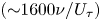 $(\mathrm{\sim }1600\nu /{U_\tau })$, respectively. An evaluation of the results indicated that this trip was not sufficient to generate a fully developed flow at the measuring section. An additional trip (denoted as T2 or T3) was used at a distance of 1 m upstream of the primary trip and the roughness height and width of this trip was varied at the two flow depths (H = 0.135 and 0.170 m). Details of the trips are provided in table 1. The flow parameters are shown only for the fully developed cases. The free-stream velocities (maximum velocities) are approximately 0.29 and 0.23 m s−1 at these two depths, which correspond to a constant value of
 $R{e_H} = 39\;000$. Reynolds numbers
 $(R{e_\theta })$ based on the momentum thickness
 $(\theta )$ (2.1) are 4205 and 3818, respectively. The experiments are carried out at a low Froude number (Fr ≈ 0.2) and the shape factors of the mean velocity profiles
 $({\delta ^\ast }/\theta )$ are approximately 1.3, where
 ${\delta ^\ast }$ is the displacement thickness (2.2)
 \begin{gather}\theta = \int_0^H {\frac{{U(x,y)}}{{{U_\infty }}}\left( {1 - \frac{{U(x,y)}}{{{U_\infty }}}} \right)\,\textrm{d}y}, \end{gather}
 \begin{gather}{\delta ^\ast } = \int_0^H {\left( {1 - \frac{{U(x,y)}}{{{U_\infty }}}} \right)\,\textrm{d}y} .\end{gather}
Details of the test conditions, trip characteristics and flow parameters.

Velocity measurements were carried out at the vertical mid-plane (x–y plane, where x and y are the streamwise and bed-normal directions, respectively) of the flume using a two-component planar particle image velocimetry (PIV) system consisting of dual pulse Nd:YAG lasers of 532 nm wavelength and 50 mJ pulse−1 with a maximum output of 800 mJ. Each laser pulse duration was 4 ns and the time interval between two pulses was set to be 2.3 ms. The laser emitter box was placed underneath the flume to illuminate the flow orthogonally from the bottom. Two cylindrical lenses with focal lengths of −15 mm and −25 mm were attached at the laser outlet to stretch the beam into a vertical laser sheet of 1 mm thickness. A spherical lens (focal length of 1000 mm) was mounted at the top of the cylindrical lenses, to maintain equal intensity at the edges of the laser sheet. A PowerViewPlus 8 MP CCD camera was installed on one side of the flume and aligned orthogonally with the laser sheet. A Nikon AF NIKKOR 50 mm f/1.8D lens was used to acquire the images of resolution 3320 pixels × 2496 pixels. The camera was operated in dual capture mode synchronized with the laser pulse repeat frequency of 2.9 Hz. Before starting the experiment, the flume water was circulated through a sand filter (~20 μm) for several days to remove unwanted particles from the tap water. The flow was then seeded with 10 μm spherical silver-coated hollow glass spheres with an effective density of 1100 kg m−3. The ability of the particles to faithfully follow the flow was assessed from the particles Stokes number (Stp) which was determined by the ratio of particle response time to turbulence time scale (Longmire & Eaton Reference Longmire and Eaton1992); Stp was found to be 5.31 × 10⁻⁵, which satisfies the criterion proposed by Clift, Grace & Weber (Reference Clift, Grace and Weber1978):  $S{t_p} \ll [2({\rho _p}/\rho ) + 1]/9 = 0.36$. The PIV image calibration was carried out by measuring the number of pixels between two dots of known distance on a calibration target. Four thousand image pairs were taken for each test condition and processed using PIVlab (Thielicke & Stamhuis Reference Thielicke and Stamhuis2014). After background subtraction, the images were pre-processed using the contrast-limited adaptive histogram equalization technique (Pizer et al. Reference Pizer, Amburn, Austin, Cromartie, Geselowitz, Greer, Ter Haar Romeny, Zimmerman and Zuiderveld1987). Intensity capping (Shavit, Lowe & Steinbuck Reference Shavit, Lowe and Steinbuck2007) and Wiener denoise filtering (Wiener Reference Wiener1964) were used to minimize the error. The particle illuminations between image pairs were correlated by a fast Fourier transform window deformation algorithm where the interrogation window of 64 × 64 pixels was reduced to 16 × 16 pixels with a spatial overlap of 50 %. The data were then post-processed using standard deviation and median filters with a predefined threshold value to remove and replace bad vectors. Less than 5 % of vectors were identified as bad and replaced by interpolated vectors. Each of the final snapshots consist of approximately 25 000 vectors at a uniform spacing of 1.3 mm in both the streamwise and wall-normal directions. MATLAB codes were developed to calculate mean and turbulence quantities, as well as for determining momentum zones and carrying out the quadrant analysis.
The reliability of the PIV measurements is highly dependent on the consistency in data acquisition and data processing. The inaccuracy in data can be quantified by uncertainty analysis that consists of bias or instrument uncertainty and precision or measurement uncertainty. Based on the studies of Forliti, Strykowski & Debatin (Reference Forliti, Strykowski and Debatin2000), Singha (Reference Singha2009), Roussinova (Reference Roussinova2009), total bias error (UNb) in the instantaneous velocity is considered to be the error in the estimation of velocity for a particle displacement of 0.1 pixel which is quantified as ±1.3 % of  ${U_\infty }$. Following the methods proposed by Coleman & Steele (Reference Coleman and Steele1995), the precision error (UNp) is calculated as t 95σ where t 95 is 1.96 corresponding to the 95 % confidence interval of the t distribution and σ is the standard deviation of the variable. The whole dataset is divided into 10 sets of 400 images and the standard deviation of all variables are calculated corresponding to each wall-normal position. The total uncertainty is estimated as
 ${(UN_b^2 + UN_p^2)^{1/2}}$ and the uncertainty corresponding to mean velocity, Reynolds normal stresses, Reynolds shear stress, skewness and flatness factor are approximately ±2 %, ±4.5 %, ±6 %, ±11 %, ±10 % of the time-averaged values of the corresponding variables, respectively. Further investigation was carried out to show the convergence of the higher-order moments and to quantify the deviation in the higher-order statistics with a change in sample size. The whole dataset was divided into five sets consisting of randomly chosen 500, 1000, 2000, 3000 and 4000 distinct samples and the flow variables were estimated for each sample size. The percentage deviation was estimated between each adjacent sample size and is presented in figure 2 to determine the convergence of the data. The deviations between two corresponding sample sizes tend to reach a converged value with the increase of sample size. For example, the mean deviation of Reynolds shear stress value between 500 and 1000 image pairs is 7 %, while it is reduced to 2 % between 3000 and 4000 image pairs. This ensures that the experimental data are within a reasonable range of variation and 4000 instances are sufficient to study the higher-order statistics for this type of flow field.
Deviation in the mean and turbulence quantities with increase in sample size.

3. Shear velocity
An accurate estimation of shear velocity is necessary for the inner scaling of the mean and turbulence parameters. In this paper, the value of  ${U_\tau }$ is estimated using a modified Clauser chart method that optimizes the double-averaged mean streamwise velocity profile (U) against the log law by an iterative curve fitting algorithm. The double-averaging technique involves both time and space averaging of the velocity data over the whole FOV (Nikora et al. Reference Nikora, Ian, Stephen, Stephen, Dubravka and Roy2007; Cameron, Nikora & Coleman Reference Cameron, Nikora and Coleman2008; Sarkar & Dey Reference Sarkar and Dey2010; Mignot, Hurther & Barthelemy Reference Mignot, Hurther and Barthelemy2011). The double averaging is carried out using the following equation:
 \begin{equation}\textrm{Double}\;\textrm{averaging}\;\textrm{of}\;p(x,y,t)\; = \frac{1}{{NL^{\prime}\; }}\sum\limits_1^N {\sum\limits_1^{L^{\prime}} {[p(x,y,t)]} }\end{equation}
where p is a variable dependent on spatial coordinates (x,y) and time (t), N is the total number of instances and  $L^{\prime}$ is the number of columns in the data matrix of each instance to cover the streamwise span of the whole FOV. Initially, the time averaging is done over 4000 instances at each data point. The time-averaged data are then spatially averaged in the streamwise direction. Thus, the whole FOV is collapsed into one double-averaged profile. In general, spatial averaging is not valid in the developing flow because the velocity profiles are varying in the streamwise direction. To check its validity, streamwise variation of time-averaged velocity and the turbulence quantities at three different vertical locations along the depth (y/H = 0.2, 0.5, 0.8) were monitored. The deviation over the 250 mm long FOV is negligible. Double averaging is used here as more data will provide better convergence of statistics of higher-order turbulence characteristics.
In the present study,  ${U_\tau }$ is determined by optimizing the functions f 1 and f 2 defined in (3.2) and (3.3). The optimization is carried out using the double-averaged mean streamwise velocity data in the range of the logarithmic layer:
 $30 \le {y^ + } \le 0.2R{e_\tau }$ (where
 $R{e_\tau } = {U_\tau }H/\upsilon $) (Balachandar & Patel Reference Balachandar and Patel2005). Initially,
 ${U_\tau }$ is calculated from the total stress in the overlap region following the equation:
 $U_\tau ^{\; 2} = (\upsilon \partial U/\partial y - \overline {u^{\prime}v^{\prime}} )$. This equation assumes a linear distribution of Reynolds shear stress throughout the depth and the value of
 ${U_\tau }$ is estimated by extrapolating the linear region of shear stress profile to the bed (Flack et al. Reference Flack, Schultz and Shapiro2005; Roussinova et al. Reference Roussinova, Biswas and Balachandar2008). However, this value is only used as an initial guess since the uncertainty in this method is high. The value of κ and B are taken as 0.41 and 5. In the beginning, the function f 1 (3.2) is optimized by a linear least squares fit in the form of y − mx = 0, forcing the intercept to be zero. The slope of this line is
 ${U_\tau }/\kappa $. In the next step, function f 2 (3.3) is optimized in a similar way to determine
 ${U_\tau }$. If both of the optimization processes provide the same value, the output is taken as the final value of
 ${U_\tau }$. Otherwise, if the difference between the two
 ${U_\tau }$ values is higher than a prescribed threshold value, the variable yo is adjusted until a good match is achieved. The parameter yo is introduced as a small correction to the y coordinate (yi) of the processed data as the location of the true y = 0 coordinate depends on the accuracy in masking the PIV images. The magnitude of yo is approximately 1.2 mm and this correction also helps to avoid the log-law mismatch near the transition region. The final y coordinates are modified with corresponding yo values as y = yi + yo
 \begin{gather}{f_1}({U_\tau }) = \frac{{\textrm{d}U}}{{\textrm{d}y}} - \frac{{{U_\tau }}}{\kappa }\frac{1}{{({y_i} + {y_o})}},\end{gather}
 \begin{gather}{f_2}({U_\tau }) = U - \frac{{{U_\tau }}}{\kappa }\ln \left[ {\frac{{({y_i} + {y_o})}}{\nu }} \right] - {U_\tau }B.\end{gather}
The values of  ${U_\tau }$ for different test conditions are presented in table 2. The deviations among them are calculated with a reference
 ${U_\tau }$ value at each depth, i.e. the test cases T1&T2 at H = 0.135 m and T1&T3 at H = 0.170 m. These two cases are fully developed conditions and will be discussed in detail in the following sections. The
 ${U_\tau }$ values for other test cases are compared with the values in corresponding fully developed states and show a variation of up to 5 %. Similarly,
 ${U_\tau }$ values for the two fully developed states are calculated for the time-averaged velocity profiles at each streamwise location and these values of
 ${U_\tau }$ (normalized by
 ${U_\infty }$) are presented in figure 3(a). The distribution of
 ${U_\tau }/{U_\infty }$ is similar in both tests and no significant variation is noticed over the span (L) of the FOV. Finally, the streamwise variation of the shape factor is presented in figure 3(b) since the integral quantity is a more reliable parameter in this context. The variation of shape factor over the FOV is found to be minor and the magnitude is close to the theoretical value of shape factor for a fully developed open channel flow which is 1.3 (shown by the dashed line in figure 3b). This ensures our expectation of the fully developed states and the validity of the double averaging.
Shear velocities for different test cases.

* Indicates fully developed conditions.
Streamwise variation of (a) normalized wall-shear velocity  $({U_\tau }/{U_\infty })$ and (b) shape factor for the fully developed states. Every seventh data point is shown for clarity.

4. Mean velocity
Mean velocity profiles for different test cases are presented with inner scaling ( ${U^ + } = U/{U_\tau }$ and
 ${y^ + } = y{U_\tau }/\upsilon $) in figure 4. A specific symbol is used for each of the four trip conditions and the velocity profiles for tests T1, T1&T2 and T1&T3 have been shifted by a constant value to enhance visualization. The dashed lines represent the log law in each case. In all cases, the mean velocity distribution shows good agreement with the log-law profile (shown by the dashed lines in figure 4) in the overlapping region. However, they start to deviate from each other near the free surface and the amount of deviation from the log law is different with different tripping conditions. The deviations are an indication that the strength of the wake changes with the change in trip size. Each of the trip conditions is likely to produce unique wake characteristics and it is difficult to identify the fully developed condition using only the log law.
Mean streamwise velocity profiles at H = 0.135 m normalized by inner scaling, compared with the log-law profile. Velocity profiles for tests T1, T1&T2 and T1&T3 are shifted vertically by a constant value to enhance visualization. The figure is generated using a subset of the total data points to avoid clutter.

As mentioned earlier, Coles (Reference Coles1956) was among the first to propose an additional term in the log law that consists of a wake strength parameter to quantify the deviation of the mean profile from the law of the wall in the defect flow region. This new equation with the additional term is widely known as the ‘velocity defect law’. The wake parameter  $\varPi$ can be derived from the upper and lower boundary conditions of velocity in the defect flow region. Several researchers have proposed different forms of the wake function (Coles Reference Coles1956; Cardoso, Graf & Gust Reference Cardoso, Graf and Gust1989; Guo, Julien & Meroney Reference Guo, Julien and Meroney2005). Based on Granville's (Reference Granville1976) formulation, Krogstad, Antonia & Browne (Reference Krogstad, Antonia and Browne1992) proposed an alternative velocity defect equation for a ZPG TBL, which can be expressed in the functional form
 $f(\varPi ) = 0$, where
 \begin{align}f(\varPi ) = \frac{{{U_\infty } - U}}{{{U_\tau }}} - \frac{{2\varPi }}{\kappa }\left[ {1 - \frac{1}{{2\varPi }}\left( {({1 + 6\varPi } ){{\left( {\frac{y}{\delta }} \right)}^2} - \; (1 + 4{\rm \pi}){{\left( {\frac{y}{\delta }} \right)}^3}} \right)} \right] - \frac{1}{\kappa }\ln \frac{y}{\delta }.\end{align}
The defect equation proposed by Krogstad et al. (Reference Krogstad, Antonia and Browne1992) consists of four unknown variables: κ,  ${U_\tau }$, δ and
 $\varPi$, and all these variables can ideally be optimized simultaneously for a given dataset. However, this optimization procedure is highly sensitive to the initial guess values and a wrong initial guess may converge the solution to an erroneous estimation of these parameters. This dependency can be made less critical by reducing the number of unknowns. Based on the discussion thus far, the magnitude of κ and
 ${U_\tau }$ are known and these variables can be removed from the optimization procedure. However, our aim is to estimate the value of
 $\varPi$ accurately without bias. The magnitude of δ varies between 0 and H and the value of
 $\varPi$ may vary significantly for any initial guess value of δ within this range. Therefore, we have chosen to use the classical definition of the boundary layer thickness to estimate δ so that the optimization process is independent of any guess value. It is worth mentioning here that the magnitude of
 $\varPi$ is still dependent on the value of κ,
 ${U_\tau }$ and δ but a small change in their values will not lead to an abrupt deviation and inaccurate estimation of
 $\varPi$ since these variables are not included in the optimization process. The magnitude of δ is determined following the standard procedure, i.e. by the bed-normal location where the mean streamwise velocity is 0.99U∞. Having set the values of κ,
 ${U_\tau }$ and δ, the value of
 $\varPi$ is estimated by minimizing function f (4.1). In figure 5(a), defect profiles for all trip conditions at a flow depth of 0.135 m are plotted against the profiles predicted from the Krogstad's defect equation (shown by the dashed lines in figure 5). The profiles for T1, T1&T2 and T1&T3 are shifted vertically by a constant value to enhance visualization. The figure shows that there is good agreement between the experimental data and the defect equation for all test cases. The wake parameter varies between 0.3 and 0.55. The Reynolds number based on displacement thickness (Reδ*) is 4200. A reasonable value of
 $\varPi$ at this value of Reδ* is 0.4 ± 0.15 as reported by several studies in open channel flow and TBLs (Balachandar & Patel Reference Balachandar and Patel2005; Chauhan et al. Reference Chauhan, Monkewitz and Nagib2009). In figure 5(a), it can be seen that the velocity defect law is corroborated by the experimental data in all cases. Since the value of
 $\varPi$ (see table inset in figure 5a) is different among the test cases, some distinction must be present in their wake characteristics. Therefore, the flow in all four tests cannot be in the fully developed state although they may follow a canonical boundary layer like behaviour. Hence, conforming to the velocity defect law is mandatory but not sufficient to ensure a fully developed state. In a standard TBL, a clear free-stream region is present where the streamwise velocity is constant, permitting a precise definition of boundary layer thickness. But in the case of open channel flow, the free surface acts as a weak wall (Nezu Reference Nezu2005) and provides a vertical constraint which may influence the inner flow significantly. This influence is more prominent when the boundary layer edge is very close to the free surface and a deduction of boundary layer thickness based on 0.99U∞ can be deceiving as seen in figure 5(a).
Collapse onto Krogstad's velocity defect law (VDL) for different trip conditions at H = 0.135 m with the normalization of y coordinate by (a) δ and (b) δ′. The profiles of T1, T1&T2 and T1&T3 are shifted by a constant value. Every fifth point is shown for clarity.

As suggested in previous studies, the boundary layer thickness is directly related to the turbulence characteristics (Balachandar & Patel Reference Balachandar and Patel2005; Flack et al. Reference Flack, Schultz and Shapiro2005; Roussinova et al. Reference Roussinova, Biswas and Balachandar2008; Marusic et al. Reference Marusic, Chauhan, Kulandaivelu and Hutchins2015). Based on this observation, the boundary layer thickness (δ′) can be redefined as the bed-normal position above which the streamwise Reynolds stress becomes constant and the turbulence intensity is minimum. The distributions of Reynolds stresses are presented in the following sections and used to determine the values of δ′ for difference test cases. The estimated boundary layer thickness based on the two definitions are compared below in table 3.
Boundary layer thickness.

With the revised definition of boundary layer thickness, the defect profiles for all test cases are presented in figure 5(b). Except for the test case T1&T2 (at H = 0.135 m), the defect profiles start to deviate from the theoretical profile near the boundary layer edge although the value of  $\varPi$ is readjusted, which establishes the presence of a unique fully developed condition. It is worth noting that the magnitude of the wake parameter (shown in the table insets in figure 5) and the boundary layer thickness (table 3) are similar in test T1&T2 for both definitions of the boundary layer thickness and the flow state in this test can be considered as the most fully developed among the four cases. However, the difference between figures 5(a) and 5(b) is minor and any conclusion made based solely on this may not be reliable. The true purpose of this analysis is to reveal the root cause of the ambiguity while matching the defect law. It is quite clear from this discussion that the corroboration of the experimental data with the log law and the defect law may not be sufficient to identify a fully developed flow if the boundary thickness is not accurately estimated. Nevertheless, when the boundary layer thickness is known, this validation is mandatory in a fully developed open channel flow.
5. Reynolds stresses and higher-order moments
The Reynolds stresses normalized by  ${U_\infty }$ and
 ${U_\tau }$ are presented for flow depths H = 0.135 m (figure 6a–c) and H = 0.170 m (figure 6d–f). A specific symbol is used for each of the four trip conditions and the fully developed states are denoted by the darker symbols (grey diamond symbols for H = 0.135 m and black square symbols for H = 0.170 m). The fully developed states are identified when the boundary layer thickness is nearly equal to the flow depth based on the value of δ′. The magnitudes of the Reynolds stresses are the highest near the wall then gradually decrease moving towards the edge of the boundary layer. The expected zero-turbulence intensity at the edge of the boundary layer seen in a standard TBL does not occur in open channel flow due to the influence of the free surface. Instead, a zone of nearly constant-turbulence intensity can be found adjacent to the free surface. The magnitude of δ′ is estimated based on the point of inflection where the slope of the profiles in the outer boundary layer changes and above which the variation in the Reynolds stresses is minimal. In figure 6, the wall-normal distributions of Reynolds stresses fall on top of each other close to bed for
 $y/H \le 0.2$ at both depths. This location is marked as A, B and C in figures 6(a), 6(b) and 6(c), respectively and they correspond to the edge of the logarithmic layer for the fully developed state. For
 $y/H\; > 0.2$, the magnitude of the Reynolds stresses gradually decreases until the boundary layer edge. Above the edge of the boundary layer, the Reynolds stresses become nearly constant which can be more prominently seen for the profiles of T0, T1 and T1&T2 at the higher flow depth (figure 6d–f). This indicates that the boundary layer thickness is at a much lower position than the flow depth and these test cases are identified as developing flow (or under-tripped cases). It is to be noticed here that the magnitude of wall-normal component of the Reynolds stress in figure 6(e) starts to decrease close to the free surface at y/H > 0.8 since the velocity fluctuations v′ must be zero at the free surface. This effect can be seen in the profiles of
 $\overline {{{v^{\prime}}^2}} $ and
 $- \overline {u^{\prime}v^{\prime}} $ for the developing test cases at the lower flow depth (T0 and T1&T2) where the magnitude reduces continuously above the boundary layer thickness instead of being constant. This is likely to happen since the thickness of the free-stream region of these test cases is much lower compared with the developing test cases of higher flow depth. However, in the fully develop test cases (T1&T2 at H = 0.135 m and T1&T3 at H = 0.170 m), the magnitude of the stresses continuously decreases linearly in the outer boundary layer up to the free surface since the boundary layer thickness is nearly equal to the flow depth. Finally, the test case T1&T3 at H = 0.135 m is identified as an over-tripped case since the turbulence generated by the trip is much higher than the fully developed flow and this excess turbulence is not dissipated over the upstream flow length. Marusic et al. (Reference Marusic, Chauhan, Kulandaivelu and Hutchins2015) have mentioned that a unique tripping is required to stimulate a well-behaved TBL flow at a specific free-stream velocity. They found a deviation from canonical behaviour when the velocity measurements are conducted close to the trip, which is equivalent to the over-tripped case T1&T3 (at H = 0.135 m) in the present study.
Distribution of normalized streamwise, bed-normal and shear stresses: (a–c) H = 0.135 m and (d–f) H = 0.170 m. Every fifth point is shown for clarity.

Based on the constant-turbulent intensity zone, the magnitude of δ′ is estimated for each test case and compared with the values of δ in table 3. Interestingly, the values of δ are in a similar range irrespective of the trip size used in the tests. When the boundary layer thickness (δ′) is estimated using the Reynolds stresses, a clear variation with tripping intensity is noticed. The magnitude of δ′ consistently increases with the increment of the trip size. While comparing the two definitions of the boundary layer thickness, the value of δ and δ′ are found to be close to each other in case of fully developed flows (T1&T2 at H = 0.135 m and T1&T3 at H = 0.17 m) and a large deviation is observed in all under-tripped cases. The test case T1&T3 at H = 0.135 m cannot be considered in this context since the flow does not retain a canonical behaviour and the value of δ′ is assumed to be equal to the flow depth. The present analysis demonstrates that a fully developed open channel flow can be stimulated experimentally by using the largest trip size that can retain the characteristics of canonical flow. For a lower trip size, the flow in the test section will be in the developing regime and the boundary layer thickness will not be of the same order as the flow depth. On the other hand, a larger trip generates excess turbulence which takes a longer streamwise length to dissipate. However, the validity of these comments depends on two parameters: (i) flow development length and (ii) aspect ratio. There must be a minimum flow development length available upstream of the test section to let the flow develop fully. Also, the aspect ratio of the flow should be high enough so that the effect of the side walls is negligible in the central region. Otherwise, if the channel is too narrow, the flow may deviate from the canonical behaviour due to secondary currents.
Velocity triple products retain the sign of velocity fluctuations and provide useful information related to coherent events. In figure 7, the bed-normal distributions of third-order moments are presented in the form of skewness which is defined as  ${S_u} = (\overline {{{u^{\prime}}^3}} )/{(\overline {{{u^{\prime}}^2}} )^{3/2}}$ and
 ${S_v} = (\; \overline {{{\nu ^{\prime}}^3}} \; )/{(\; \overline {{{\nu ^{\prime}}^2}} )^{3/2}}$. The value of skewness of a normal distribution is zero due to symmetry in the distribution of the data points. Any value apart from zero reveals temporal asymmetry in the signal (Balachandar & Bhuiyan Reference Balachandar and Bhuiyan2007), which is directly related to the turbulence characteristics of the flow. In figure 7(a,e),
 ${S_u}$ shifts from a positive to a negative value close to the bed, then continuously decreases in the upward direction away from the bed until it reaches a peak value. This represents a strong directional preference by the higher magnitude of the velocity fluctuations of extreme events, indicating a strong coherence in the flow structures. On the other hand, the
 ${S_v}$ profiles (figure 7b,f) also show a similar trend although the skewness value is positive throughout the depth except near the bed. Above the point of maximum skewness, the skewness value reduces and finally reverts back to zero (or a very small value) at a specific height based on the tripping intensity (except the over-tripped case). These specific bed-normal coordinates above which the skewness values are nearly constant can represent the edge of the boundary layer and the value of δ′ so determined is consistent with the Reynolds stress profiles. Since, the distribution of
 $u^{\prime}$ is negatively skewed and of
 $v^{\prime}$ is positively skewed, the shear stress contribution by ejections is likely to be higher than the sweep events in the boundary layer except in the region very close to the bed and this is consistent with the canonical behaviour of a boundary layer flow (Flack et al. Reference Flack, Schultz and Shapiro2005; Roussinova et al. Reference Roussinova, Biswas and Balachandar2008). However, in the over-tripped case (T1&T3 at H = 0.135 m),
 $|{S_u}|$ continuously increases up to the free surface due to excess turbulence generated by the trip which can be distributed in the vertical direction and create free surface perturbations. This behaviour is consistent with what is seen in figure 6(a), where the Reynolds stress at the free surface is found to be much higher than in the other test cases.
Distribution of normalized third-order and fourth-order moments: (a–d) H = 0.135 m and (e–h) H = 0.170 m. Every fifth point is shown for clarity.

Similarly, fourth-order turbulence statistics are illustrated in figure 7(c,d,g,h) in the form of flatness factors, defined as  ${F_u} = (\overline {{{u^{\prime}}^4}} )/{(\; \overline {{{u^{\prime}}^2}} )^2}$ and
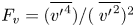 ${F_v} = (\overline {{{v^{\prime}}^4}} )/{(\; \overline {{{v^{\prime}}^2}} )^2}$. The flatness value of three corresponds to the normal distribution. Any value other than three describes the nature of intermittency in the distribution of the velocity (Balachandar & Bhuiyan Reference Balachandar and Bhuiyan2007). The curves in figure 7(c,d,g,h) show that the flatness profiles have a peak in a similar location as the skewness profiles which implies that the quadrant events make strong intermittent contributions to the turbulence production (Grass Reference Grass1971). Except for the over-tripped case, Fu has a value close to three near the bed, then gradually increases to the peak value and returns to three at the water surface. However, in the over-tripped case (T1&T3 at H = 0.135 m), Fu and Fv are close to three throughout the depth except near the free surface.
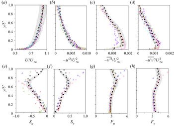
To check for similarity between the two fully developed flows, the bed-normal distribution of the flow variables of test cases T1&T2 at H = 0.135 m and T1&T3 at H = 0.170 m are compared in figure 8 along with the velocity data of previous research (see table 4 for details). For the present experimental data, δ′ is used as the scaling factor of the y coordinates as it provides an accurate estimation of boundary layer thickness. The grey region represents a deviation of ±10 % from the fully developed flow data at H = 0.170 m which are used to demonstrate the range of variability among the datasets. In each of the graphs, the fully developed profiles collapse onto each other and show good agreement with the datasets of previous research, confirming the validity of the current definition of boundary layer thickness based on the distributions of Reynolds stresses. This implies that identification of the fully developed flow in the current research is accurate and δ′ can be used as the proper length scale and a viable parameter for defining boundary layer thickness. It is to be noticed here that the distributions of skewness and flatness show a difference in magnitude between the present fully developed flow data and the standard TBL results near the edge of the boundary layer and this is expected due to the influence of the vertical restriction provided by the free surface (figures 8e,f,g,h).
Comparison of fully developed profiles with previous studies: (a) mean streamwise velocity  $(U/{U_\infty })$, (b–d) Reynolds stresses
 $(\overline {{{u^{\prime}}^2}} /U_\infty ^{\; 2},\overline {{{v^{\prime}}^2}} /U_\infty ^{\; 2}, - \overline {u^{\prime}v^{\prime}} /U_\infty ^2)$, (e–h) third- and fourth-order moments of streamwise velocity fluctuation (Su, Sv, Fu, Fv). The grey region presents a variation of ±10 % from the fully developed flow data of test case T1&T3 at H = 0.170 m. Every seventh point of the current experimental data is shown for clarity.

Details of previous studies used to check the self-similarity of the fully developed state (OCF: open channel flow, CF: channel flow, TBL: turbulent boundary layer).

6. Uniform momentum zones
In the previous sections, the role of the trip size in accurately stimulating the flow to a fully developed state was provided by observing the distributions of Reynolds stresses and higher-order moments. Once the fully developed state is ensured, different aspects of the flow can now be characterized using the uniform momentum zone (UMZ) analysis. In incompressible flows, UMZs can be simply defined as the zones of similar streamwise velocity (Adrian et al. Reference Adrian, Meinhart and Tomkins2000). The streamwise momentum is nearly constant within such a zone and the velocity variation between adjacent zones is higher than the velocity fluctuation within a zone. As suggested by de Silva et al. (Reference de Silva, Hutchins and Marusic2016), these zones of uniform momentum are identified by the peaks in the probability density function (PDF) generated by the instantaneous streamwise vectors below the TNTI. The details of the detection methodology for determining TNTI position and the UMZs are provided in the following sections.
6.1. Detection of the TNTI
The TNTI is a thin zone that separates the region of significant turbulence from the region of negligible turbulence. Detecting the location of the TNTI is essential to eliminate the irrotational non-turbulent region from the momentum zone analysis. UMZs are identified by the local maxima in the PDF of the instantaneous streamwise velocities. If the velocity values in the non-turbulent zone are not removed, there is a possibility of having a large outer peak in the PDF which may overshadow the smaller peaks inside the turbulent domain. These peaks correspond to the region with higher momentum, but with insignificant contribution to turbulence generation (de Silva et al. Reference de Silva, Hutchins and Marusic2016).
The detection criteria for the TNTI have been an issue of debate among researchers for years. One of the well-established methods of identifying the TNTI is to consider the vorticity distribution and this method is widely used in jet studies. However, it is more difficult to implement this criterion in boundary layer type flows because of the noisy free stream (Laskari et al. Reference Laskari, de Kat, Hearst and Ganapathisubramani2018). The method of local instantaneous kinetic energy deficit as described in Chauhan, Philip & Marusic (Reference Chauhan, Philip and Marusic2014a), Chauhan et al. (Reference Chauhan, Philip, de Silva, Hutchins and Marusic2014b) has been suggested to eliminate any effect of external perturbations. However, this method was tested and found to be well suited for TBL flows where a significant domain of free stream is present. In open channel flows, the influence of free surface must be taken into consideration, especially in the case of fully developed state where the edge of the boundary layer is very close to the free surface. Therefore, we propose a modified form of the equation suggested by Chauhan et al. (Reference Chauhan, Philip and Marusic2014a,Reference Chauhan, Philip, de Silva, Hutchins and Marusicb) where the wall-normal free-stream velocity  $({V_\infty })$ is also taken into consideration along with the streamwise velocity
 $({U_\infty })$ for better accuracy. Here,
 ${U_\infty }$ and
 ${V_\infty }$ are taken as the velocity at the edge of the boundary layer to maintain consistency. It must be noted here that the magnitude of
 ${V_\infty }$ in the free-stream region should ideally be zero, which is practically not true in open channel flow due to the influence of free surface. The kinetic energy deficit (K) at each point of the flow domain is calculated with respect to a reference frame that is moving with the mean free-stream velocity
 $({U_\infty },{V_\infty })$. For each point on the grid, the average energy deficit over a 3 × 3 window (all surrounding points) is computed by modifying the equation of Chauhan et al. (Reference Chauhan, Philip and Marusic2014a,Reference Chauhan, Philip, de Silva, Hutchins and Marusicb) as
 \begin{equation}K = 100 \times \frac{1}{{9(U_\infty ^2 + V_\infty ^2)}}\sum\limits_{m,n ={-} 1}^1 {[{{({U_{m,n}} - {U_\infty })}^2} + {{({V_{m,n}} - {V_\infty })}^2}]} .\end{equation}
Once the kinetic energy deficit is calculated throughout the flow domain, a threshold value (Kth) is required to demarcate between the turbulent and the non-turbulent flow. A domain inside the FOV corresponds to the non-turbulent zone if K is lower than the threshold value and to the zone of significant turbulence if K is higher. Therefore, a variable (Kb) is defined in such a way that it is zero in the turbulent zone and one in the non-turbulent zone. A contour algorithm is employed to estimate the Kb = 0.5 contour line which represents the TNTI location. The wall-normal coordinates of the local TNTI positions are extracted from all instances and used to calculate the mean  ${Y_{TNTI}}$ and standard deviation (σ). Chauhan et al. (Reference Chauhan, Philip, de Silva, Hutchins and Marusic2014b) initially defined the magnitude of Kth to be equal to the free-stream turbulent intensity and then increased by a small amount to match
 ${Y_{TNTI}} + 3\sigma \approx \delta $, since they assumed a Gaussian distribution with a 95 % confidence interval. Laskari et al. (Reference Laskari, de Kat, Hearst and Ganapathisubramani2018) reported setting Kth in such a way so that the intermittency profile is constant above δ and
 ${Y_{TNTI}} + 3\sigma < 1.4\delta $. A similar approach is adapted in the present research where
 ${Y_{TNTI}}$ is calculated over a range of threshold values (0.2 ≤ Kth ≤ 5.0). The final value of Kth is determined to be 0.9 for which
 ${Y_{TNTI}} + 3\sigma \le \delta ^{\prime}$ in the fully developed test cases. In figure 9, the magnitudes of
 ${Y_{TNTI}}$ are plotted against the corresponding threshold values for all test cases. Interestingly, all the profiles collapse onto each other when Kth is higher than 0.9 but deviate significantly for a threshold value lower than 0.9. Therefore, this value is likely to provide an optimum estimation of Kth which differentiates two different types of attributes in the flow field in terms of TNTI positions. If the value of Kth was chosen to be much smaller (i.e. of the order of free surface turbulence intensity), the TNTI location will be highly sensitive to the value of Kth since the variation of K is small near the free surface because the mean velocity components are close to
 ${U_\infty }$ and
 ${V_\infty }$. Consequently, any external noise and free surface perturbation will have a strong influence on the location of the TNTI. On the other hand, if Kth is set to be a much larger value, the TNTI will be at a lower position and important information on turbulence and momentum transfer will be lost in the outer domain. Furthermore, the effect of a smaller variation (up to 20 %) in the value of Kth was tested by carrying out the momentum zone analysis for five values of Kth (0.7, 0.8, 0.9, 1.0, 1.1) and the number of momentum zones (NUMZ) was found to be similar in each case (see Appendix A). Therefore, a small variation in the value of Kth has only a minor influence on the UMZ analysis and cannot alter the findings that are achieved by keeping a constant value of Kth as 0.9 for all test cases. This value is used in all further analyses on UMZs. The wall-normal positions of TNTI are determined using this threshold value of K and the probability distribution of
 ${Y_{TNTI}}$ over 4000 snapshots is presented in figure 9(b) for test cases T0 and T1&T3 at H = 0.170 m. In both cases, the probability distributions are skewed towards the bottom wall, similar to what was observed by Laskari et al. (Reference Laskari, de Kat, Hearst and Ganapathisubramani2018) and the magnitude of the skewness for the developing flow (skewness = 2.8) is higher compared with the fully developed state (skewness = 0.8).
(a) Normalized mean TNTI location  $({Y_{TNTI}})$ for all test cases at H = 0.170 m and the distribution of
 ${Y_{TNTI}} + 3\sigma $ for the fully developed state T1&T3 (inset) corresponding to a value of Kth between 0.3 to 5.0. (b) The probability distribution of
 ${Y_{TNTI}}$ for test cases T0 and T1&T3 at H = 0.170 m, estimated using Kth = 0.9.

6.2. Detection of UMZs
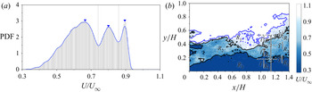
The UMZs are detected by the PDF of instantaneous streamwise velocity vectors that lies inside the turbulent region i.e. the region in the FOV where K is greater than Kth. The probability densities are determined by dividing the velocity data of each instance (U) into small bins, and the bars corresponding to each bin in the velocity histogram (figure 10a) represent the probability that the velocity lies in that specific bin. The peak probability density values (as shown by ‘▾ - blue’ in figure 10a) in the histogram correspond to each of the momentum zones and the value of  $U/{U_\infty }$ corresponding to each peak is the modal velocity (MV) of that zone. Each peak is confined by two local minima and these minimum values are used as the contour levels of the momentum zones. These contour lines demarcate the area of each momentum zone and are presented in figure 10(b). The blue contour line in figure 10(b) represents the location of TNTI at the specific instance, whereas the black line separates two momentum zones. The zones are ranked
 $({R_i})$ based on their bed-normal position, i.e. the UMZ adjacent to the TNTI is ranked one and that adjacent to the bed is ranked the highest. The value of highest rank depends on the number of UMZs present in that specific instance. The average bed-normal position (i.e. the adjacent upper contour level) and the thickness of the momentum zones are represented by
 ${Y_{UMZ}}{|_{{R_i}}}$ and
 ${t_{UMZ}}{|_{{R_i}}}$ where i is the rank of the corresponding momentum zone.
(a) PDF of streamwise velocities below TNTI for a single instance. The inverted triangles ‘▾ - blue’ indicate the modal velocities and the dashed lines differentiate the UMZs. The continuous blue line represents the curve fitted over the probability data to find the modal velocities. (b) Corresponding contour plot of the UMZs. The average bed-normal position (i.e. the adjacent upper contour level) and the thickness of the momentum zones are presented by  ${Y_{UMZ}}{|_{{R_i}}}$ and
 ${t_{UMZ}}{|_{{R_i}}}$, where i is the rank of the corresponding momentum zone.

The instances with a similar number of peaks in the PDF (i.e. a similar number of UMZs) are likely to have a similar type of coherent event. As shown by Laskari et al. (Reference Laskari, de Kat, Hearst and Ganapathisubramani2018), the large-scale Q2 and Q4 events are associated with the instances of higher and lower than average number of momentum zones, respectively. The variation in flow characteristics with the change in number of momentum zones (NUMZ) is shown in the following sections by conditional averaging of flow variables of the instances that belong to a similar number of momentum zones. Therefore, some important considerations must be taken to ensure a consistent identification of the magnitude of NUMZ. Firstly, an optimum selection of the bin size is mandatory in this context since the number of momentum zones may vary significantly with the bin size. Similar to Laskari et al. (Reference Laskari, de Kat, Hearst and Ganapathisubramani2018), a bin size of  $0.5{U_\tau }$ is used here for a range of velocities,
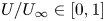 $U/{U_\infty } \in [0,1]$. However, a non-zero probability density is found only in the range,
 $U/{U_\infty } \in [0.25,1]$ since the flow velocities very close to the bed cannot be captured due to the spatial resolution of the data acquisition tool. A smaller and a larger bin size (
 $0.25{U_\tau }$ and
 $0.75{U_\tau }$) were also employed for a similar UMZ analysis to study the influence of bin size on the momentum zone analysis. A consistent output is attained for these two bin sizes (see Appendix B) and the current selection of the bin size is not likely to alter the findings of this paper.
The method of identifying UMZ contour levels is also dependent on the length of the FOV (L) and the number of vectors taken into consideration. Adrian et al. (Reference Adrian, Meinhart and Tomkins2000) and de Silva et al. (Reference de Silva, Hutchins and Marusic2016) have chosen a streamwise length of δ, which corresponds to a viscous wall unit  ${L^ + } = L{U_\tau }/\upsilon = 2000$. Laskari et al. (Reference Laskari, de Kat, Hearst and Ganapathisubramani2018) have also used a similar L + instead of using the whole FOV for better comparability. In the present analysis, the streamwise extent of the FOV is approximately 250 mm (~1.4H) that corresponds to 2250 viscous wall units and approximately 25 000 vectors are present in every snapshot with a spatial resolution of ~1.3 mm. Since the value of L + corresponding to the whole FOV is in a similar range as mentioned in the previous research, we have chosen to use the whole FOV at the highest data resolution for maximum utilization of our data. Further, the momentum zone analysis is also carried out varying the length of the FOV in the range of 1250 ≤ L + ≤ 2250 at similar data resolution, which reduces the number of vectors present in the FOV keeping the vector density the same. A minor variation in the number of momentum zones is noticed with the change in streamwise extent of the FOV, but this has a negligible impact on the qualitative trend of the dataset (see Appendix A).
Once the PDFs of the velocity data are generated, a peak-detection algorithm is required to identify the modal velocities and eliminate other minor peaks. A moving-average filter and a weighted linear least square based local regression algorithm are used to fit a smooth curve (shown by the blue line in figure 10a) over the data points (bi, Pi) where bi is the ith bin and Pi is the corresponding probability density. As suggested by Laskari et al. (Reference Laskari, de Kat, Hearst and Ganapathisubramani2018) and Chen et al. (Reference Chen, Chung and Wan2020), the algorithm involves filtering using three important criteria:  ${F_d}$ (allowed distance between two peaks),
 ${F_h}$ (minimum of the height of each peak) and
 ${F_p}$ (prominence of each peak based on the relative height to its neighbouring bins). The peaks in the PDF diagram are only recognized if
 ${F_d} > 5$ bins (~10 % of
 ${U_\infty }$),
 ${F_h} > 1$ and
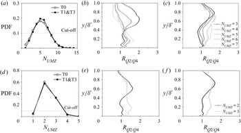
 ${F_p} > 25\,\%$. The validity of this algorithm is also taken into consideration while adjusting the bin size and the value of these thresholding parameters are finely adjusted to get the best output. This process merges the peaks in close proximity and removes the peaks whose relative probability density is not significantly higher than the neighbouring bins. The peaks corresponding to very small probability density are also eliminated, which also discards any minor peaks generated artificially by the curve fitting algorithm. The PDF of NUMZ is estimated by identifying the peaks using this algorithm and presented in figure 11(a). A maximum of 6 peaks are identified over 4000 instances. The instances corresponding to NUMZ between 2 and 4 are considered for the UMZ analysis based on a cutoff of the probability density value of 0.1 (10 % of overall dataset) since conditional averaging over a small dataset will not provide a consistent comparison of the flow characteristics. The accuracy of the peak-detection algorithm is tested by estimating the mean contour levels corresponding to the average bed-normal positions of UMZs
 $({Y_{UMZ}}{|_{{R_i}}})$ and the modal velocities
 $({Y_{MV}}{|_{{R_i}}})$. It is to be noticed here that
 ${Y_{UMZ}}$ represents the wall-normal position of upper edge of the corresponding momentum zone, whereas,
 ${Y_{MV}}$ is estimated by extracting the wall-normal position of the velocity contours corresponding to the modal velocities of specific momentum zones. The distribution of
 ${Y_{UMZ}}{|_{{R_i}}}$ and
 ${Y_{MV}}{|_{{R_i}}}$ (shown by ‘
 $\bullet$ - black’ and ‘▴ - ash’, respectively) are presented in figure 11 for the fully developed flow (test case T1&T3 at H = 0.17 m). The circles at the highest bed-normal positions indicate the position of the TNTI of the corresponding column. The space between two circles or a circle and the bottom wall in each column represents the average thickness of each of the momentum zones. The average momentum zone thickness gradually decreases with the events of larger number of peaks which helps in accommodating more layers of UMZs. In each case, the average wall-normal positions of the MV contour levels lie within the corresponding momentum zones showing a consistent behaviour and proving validity of the peak-detection algorithm. Here, YUMZ and YMV are determined based on the mean wall-normal positions of the contour lines at each instance which correspond to the minima and maxima of the PDF diagram of the instantaneous velocities (such as in figure 10a), respectively. At each instant, the velocity magnitude of the MV is limited by the minima around it. When a time averaging of a number of instances is carried out, it is not mandatory that the mean wall-normal position of the contour line corresponding to the MV will lie in between the contour lines corresponding to the velocity minima. This depends on several parameters, such as velocity distribution in instantaneous snapshots, adequacy of the bin size, accuracy in identifying the distinct peaks, accuracy in extracting the wall-normal coordinate of the contour lines etc. In the present experimental data, YMV always lies in between two YUMZ which proves the accuracy and validity of the analysis.
(a) PDF of NUMZ corresponding to bin size  $0.5{U_\tau }$; (b) bed-normal distributions of
 ${Y_{UMZ}}{|_{{R_i}}}$ and
 ${Y_{MV}}{|_{{R_i}}}$ (shown by ‘
 $\bullet$ - black’ and ‘▴ - ash’, respectively) for the fully developed flow (test case T1&T3 at H = 0.170 m). The subscript i indicates the value of the rank.

6.3. Characterization of fully developed flow
In this section, flow properties of the fully developed open channel flow (test case T1&T3 at H = 0.17 m) is characterised by analysing different attributes of the momentum zones. As mentioned earlier, the velocity data of each instance are used to generate the PDFs and the number of peaks in the PDF indicates the number of momentum zones present at that particular instance. The momentum zones at each instance are ranked based on their bed-normal position. For example, if the PDF of velocity data of a specific instance correspond to NUMZ = 3, there will be three momentum zones which are ranked one to three. The rank is one for the zone at the highest bed-normal position and three for the zone closest to the bed. The instances with similar number of UMZs are grouped together to see an overall characteristic of these events. The normalized mean modal velocities  $({U_{MV}}{|_{{R_i}}})$, UMZ contour levels
 $({Y_{UMZ}}{|_{{R_i}}})$ and momentum zone thickness
 $({t_{UMZ}}{|_{{R_i}}})$ of each group are estimated by the conditional averaging of the data corresponding to their ranks and presented in figure 12(a–c). The data corresponding to a specific value of NUMZ are represented by the same colour and the data of the same rank are shown by similar markers. Each of the markers indicate the mean values of modal velocities and the bar represents the distribution around the mean value. The length of the bar is estimated by the magnitudes of the 25th and 75th percentiles of the distribution, which show the extent of centred 50 % of the data. The PDFs in figure 12(c–e) represent one such example of the distribution of
 ${U_{MV}}$,
 ${Y_{UMZ}}$ and
 ${t_{UMZ}}$ for
 ${R_1}$ at NUMZ = 3 and the corresponding 25th and 75th percentile positions are marked with the dashed lines.
Conditional averaging of the data corresponding to a specific value of NUMZ based on their rank  $({R_i})$ of (a) modal velocities
 $({U_{MV}}{|_{{R_i}}})$, (b) bed-normal position of the mean contour level of UMZs
 $({Y_{UMZ}}{|_{{R_i}}})$ and (c) the corresponding thickness of UMZs
 $({t_{UMZ}}{|_{{R_i}}})$. Same markers are used for the same rank whereas similar colours are used for a specific value of NUMZ. The markers represent the centred values and the bars show the distribution around the centred value based on the magnitude of 25th and 75th percentiles. The distributions corresponding to NUMZ = 3 are presented for (d)
 ${U_{MV}}{|_{{R_1}}}$, (e)
 ${Y_{UMZ}}{|_{{R_1}}}$ and (f)
 ${t_{UMZ}}{|_{{R_1}}}$. The magnitudes of the 25th and 75th percentiles are shown by the dashed lines and the zone between them presents the centred 50 % of the data.

The centred value and the distributions of  ${U_{MV}}$,
 ${Y_{UMZ}}$ and
 ${t_{UMZ}}$ are used to predict the flow characteristics and fluid motions. Although, the present experimental data are not time resolved (data acquisition rate 2.9 Hz), these predictions are made based on the similarity with the analyses of time-resolved data acquired by Laskari et al. (Reference Laskari, de Kat, Hearst and Ganapathisubramani2018) and Chen et al. (Reference Chen, Chung and Wan2020). The magnitudes of
 ${U_{MV}}$ and
 ${Y_{UMZ}}$ for
 ${R_1}$ are nearly constant (figure 12a,b) although the distribution around the centred value gradually reduces when the number of momentum zones increases. There is only the possibility of less variation since the thickness of the momentum zones for
 ${R_1}$ significantly reduces (figure 12c) with the increment of NUMZ to accommodate the additional zones. On the other hand, the magnitudes of
 ${U_{MV}}$ and
 ${Y_{UMZ}}$ for
 ${R_2}$ and
 ${R_3}$ increase significantly with the increment of NUMZ keeping the thickness similar, which indicates the zones corresponding to
 ${R_2}$ and
 ${R_3}$ move upwards and this cause shrinking of the outer-most momentum zone. The difference in magnitudes of the adjacent
 ${U_{MV}}$ and
 ${Y_{UMZ}}$ values at a specific NUMZ also reduces to accommodate this new zone. This indicates that the new zone appears near the bed which is consistent with the observations of Laskari et al. (Reference Laskari, de Kat, Hearst and Ganapathisubramani2018) and Chen et al. (Reference Chen, Chung and Wan2020). Since the fluid parcels near the bed are lifted upward, they gain higher momentum in this process. This upward movement of slow-moving fluid towards the zone of higher momentum reveals the existence of large-scale Q2 events near the bed. On the contrary, if we consider a transition from higher NUMZ to a lower value, the existence of large-scale Q4 events can be found. When a momentum zone disappears, the MV of a similar ranked UMZ reduces and it moves towards the bed, which indicates the downward motion of higher momentum fluid parcels or large-scale sweeping motion near the bed. Therefore, instances with higher number of momentum zones are likely to be highly influenced by large-scale Q2 events, whereas large-scale Q4 events are dominant in the case of a smaller number of momentum zones. Interestingly, these large-scale fluid motions can be found very close to the bed, possibly within the logarithmic layer and the flow in the domain above shows different characteristics. For example, the magnitudes of
 ${U_{MV}}$ and
 ${Y_{UMZ}}$ for
 ${R_i} > 1$ increase significantly with an increment in NUMZ, whereas they are nearly constant for
 ${R_i} = 1$. But in case of a canonical boundary layer flow, similar characteristics as seen in
 ${R_i} > 1$ are found for UMZs at any rank (Laskari et al. Reference Laskari, de Kat, Hearst and Ganapathisubramani2018) which can be safely assumed to be equivalent to the developing flow in test T0. Therefore, it can be concluded that there is a possibility of variation in characteristics between the developing and the fully developed open channel flows and this aspect is further explored in the following sections using quadrant analysis.
7. Comparison of developing and developed flow
In fully developed open channel flow, the boundary layer thickness is nearly equal to the flow depth, which imposes a restriction on the transfer of turbulence and momentum by the free surface. This may cause an internal heterogeneity in the flow characteristics and affect the hierarchical pattern of the energy distribution. To characterize any differences, a developing case is compared with a fully developed case. To this end, the UMZs of the streamwise velocities in the fully developed state (test case T1&T3 at H = 0.170 m depth) are compared with that of the developing flow (test case T0 at H = 0.170 m depth). The objective of this comparison is to bring forth the variation in flow characteristics if tripping is not adequate or the flow is not fully developed. The test case T0 is chosen as the developing flow since this is the closest representation of a standard TBL among the four test cases with a clear free stream. The boundary layer thickness in case T0 is nearly half of the flow depth, enabling a momentum exchange between the boundary layer and free stream without any large influence from the free surface. This comparison demonstrates the effect of the free surface on the variation of instantaneous boundary layer flow variables and quadrant events in fully developed open channel flow.
7.1. Quadrant events
Herein, the focus of the quadrant analysis is to connect the momentum zone analysis with the dynamics of ejections and sweeps, and the traditional quadrant analysis procedure of Lu & Willmarth (Reference Lu and Willmarth1973) is followed. Reynolds stresses at each point are calculated and assigned to the corresponding quadrants by the sign of the velocity fluctuations u′ and v′. The velocity fluctuations are calculated by subtracting the globally averaged (i.e. time averaged over 4000 snapshots) from the instantaneous velocities. The second quadrant (Q2) corresponds to ejections (u′ < 0, v′ > 0) while the fourth (Q4) relates to sweeps (u′ > 0, v′ < 0). Total shear stress contribution from each quadrant and to a specific value of NUMZ is calculated using the following equation:
 \begin{equation}{\overline {u^{\prime}v^{\prime}} _{Qi}}{|_{{N_{UMZ}}}} = \frac{1}{{{n_{UMZ}}L^{\prime}\; }}\mathop \sum \limits_1^{{n_{UMZ}}} \mathop \sum \limits_1^{L^{\prime}} {[u^{\prime}(x,y,t)v^{\prime}(x,y,t)]_{Qi}}\quad \textrm{for}\;i = 2\;\textrm{or}\;4,\end{equation}
where  ${n_{UMZ}}$ is the number of instances corresponding to a specific NUMZ and
 $L^{\prime}$ is the number of columns in the data matrix of each instance to cover the streamwise span of the whole FOV. The hole size is set to be zero so as to include the contributions from all events and not just the extreme events. In order to determine the dominant quadrant events with a variation in NUMZ, the ratio of shear stress contributions from Q2 and Q4
 $({R_{Q2/Q4}} = {\overline {u^{\prime}v^{\prime}} _{Q2}}{|_{{N_{UMZ}}}}/{\overline {u^{\prime}v^{\prime}} _{Q4}}{|_{{N_{UMZ}}}})$ is presented in figure 13 for both the developed (T1&T3 at H = 0.17 m) and the developing flow (T0 at H = 0.17 m).
(a) PDF of NUMZ corresponding to bin size 0.5Uτ for the developing flow (T0 at H = 0.170 m) and the fully developed flow (T1&T3 at H = 0.170 m). Distributions of conditionally averaged (based on the value of NUMZ) ratio of shear stress contribution from Q2 and Q4 events for (b) the fully developed flow and (c) the developing flow. For clarity, plots are generated using a subset of total data points. In (b,c), every fifth point is shown.

Firstly, the PDFs of NUMZ for both cases are presented in figure 13(a) to provide a comparison between the probability of occurrence of instances corresponding to different number of peaks in the PDF. Interestingly, a similar number of instances (out of total 4000 instances) corresponding to a specific value of NUMZ are found for both the developed and developing flow which can be seen in the probability distribution in figure 13(a). A cutoff probability density value of 0.1 is implemented here and the instances with NUMZ = 2, 3 and 4 are taken into consideration for further analyses. The ratio of  ${\overline {u^{\prime}v^{\prime}} _{Q2}}$ and
 ${\overline {u^{\prime}v^{\prime}} _{Q4}}$ provides an indication of the dominant event, i.e. the maximum shear stress is generated by the ejection events if RQ 2/Q4 > 1 and by the sweep events when RQ 2/Q4 < 1. The bed-normal distribution of RQ 2/Q4 is presented for both the fully developed flow (figure 13b) and the developing flow (figure 13c). The fully developed flow shows a vertical variability of the coherent events. For NUMZ = 2, the magnitude of RQ 2/Q4 is the highest at
 $y/\delta ^{\prime} \approx 0.6$ and indicates strong dominance of ejections over sweeps at this depth. Below this depth, the value of RQ 2/Q4 gradually decreases and becomes nearly equal to one near the bed
 $(y/\delta ^{\prime} < 0.3)\; $. However, in the case of NUMZ = 4, the bed-normal position of this peak value of RQ 2/Q4 moves towards the bed
 $(y/\delta ^{\prime} \approx 0.2)$ and the value of RQ 2/Q4 is nearly equal to one at
 $y/\delta ^{\prime} > 0.35\; $. The distribution of NUMZ = 3 provides an intermediate characteristic exhibiting two peaks at
 $y/\delta ^{\prime} \approx 0.6$ and
 $y/\delta ^{\prime} \approx 0.2$. In the case of developing flow, the maximum value of RQ 2/Q4 is observed near
 $y/\delta ^{\prime} \approx 0.75$ (irrespective of the number of momentum zones) which is much closer to the boundary layer thickness in comparison with the fully developed flow and the distributions of NUMZ = 2, 3 and 4 appear to be similar in pattern. Some similarity with the developed flow can be seen since the magnitude of RQ 2/Q4 gradually decreases in the range
 $0.45 < y/\delta ^{\prime} < 1.0$ and increases in the lower flow domain with the increment of NUMZ. However, the vertical shifting of the peak value of RQ 2/Q4 is not present in the developing flow. This comparison of vertical variability can be more prominently seen when the bin size is reduced to 0.25Uτ and a higher range of values of NUMZ is available (see Appendix B). However, we choose to present the results corresponding to the bin size 0.5Uτ since a higher number of instances are present corresponding to each value of NUMZ making this analysis more reliable. Also, the peak-detection algorithm may provide some inconsistency in determining the number of peaks for some specific instances for a smaller bin size, although this is unlikely to alter the overall conclusion.
7.2. Velocity deficits
In the previous analysis, the shear stress contributions to the ejections and sweeps are determined based on the instantaneous velocity fluctuations at each point. In the present section, the main objective is to depict the large-scale fluid motions by the distributions of instantaneous velocity deficits which are estimated as  ${U_{def}} = {U_{DA}}{|_{{N_{UMZ}}}} - {U_{DA}}$ and
 ${V_{def}} = {V_{DA}}{|_{{N_{UMZ}}}} - {V_{DA}}$, where UDA and VDA are double-averaged velocity for all 4000 snapshots and
 ${U_{DA}}{|_{{N_{UMZ}}}}$ and
 ${U_{DA}}{|_{{N_{UMZ}}}}$ indicate the conditionally double-averaged velocities over the instances for a specific value of NUMZ. The distribution of the normalized streamwise and bed-normal velocity deficits (Udef /U∞ and Vdef /U∞) are presented for the fully developed flow in figure 14(a,b) and the developing flow in figure 14(c,d). Based on the signs of the velocity deficits at a specific zone inside the flow domain, the large-scale fluid motions can be identified. In the wall-normal profiles of velocity deficit, if there is significant region with Udef < 0 and Vdef > 0, this indicates the existence of large-scale Q2 events and similarly, large-scale Q4 events can be identified if there is a significant region for Udef > 0 and Vdef < 0. For NUMZ = 2 (i.e. for a lower number of momentum zones), the streamwise velocity deficit is positive and the bed-normal velocity deficit is mostly negative near the bottom wall (approximately at
 $y/\delta ^{\prime} \le 0.4$), which indicates the existence of large-scale Q4 events. Correspondingly, for a higher number
 ${U_{def}}$ is negative and
 ${V_{def}}$ is positive which shows the presence of large-scale Q2 events near the bed. Near the bed, this variation in large-scale fluid motion with the change in number of momentum zones is present in both the fully developed and the developing flow. However, in the case of fully developed flow, an opposite nature of large-scale fluid motion is also observed within the boundary layer above
 $y/\delta ^{\prime} = 0.4$, i.e. large-scale Q4 events are present for a higher number of momentum zones and large-scale Q2 events for a lower number of momentum zones. This opposing characteristic between the logarithmic layer and the flow domain above it is not prominent in the developing flow. The magnitudes of the streamwise velocity deficits in developing flow are nearly zero at
 $y/\delta ^{\prime} \ge 0.6$ (figure 14c), which is similar to the findings of Laskari et al. (Reference Laskari, de Kat, Hearst and Ganapathisubramani2018). However, the bed-normal velocity deficit profiles in the developing flow (figure 14d) corresponding to NUMZ = 2 and 4 are clearly not zero and change signs approximately at
 $y/\delta ^{\prime} = 0.5$, since the boundary layer flow in the developing state may also have some influence of the free surface. In open channel flow, the constraint imposed by the free surface always exists although its influence on the flow varies depending on the bed-normal position of the edge of the boundary layer relative to the flow depth.
Distributions of conditionally averaged (based on the value of NUMZ) normalized streamwise and wall-normal velocity deficit for (a,b) the fully developed flow (T1&T3 at H = 0.170 m) and (c,d) the developing (T0 at H = 0.170 m). Every fifth point is shown for clarity.

It is seen in the present analysis that the large-scale fluid motion near the wall is comparable between the developing and the developed flow since the effect of vertical constraint provided by the free surface is negligible in this region. Moving upward, the effect of free surface becomes more prominent, especially in the fully developed state. Since there is no free-stream region in the fully developed state, no vertical momentum exchange is possible at the edge of the boundary layer. Therefore, additional turbulence in the outer boundary layer (for example, a patch of ejected fluid) must be dispersed through the surrounding fluid, which may cause internal fluid motion which is likely to cause an opposing large-scale fluid motion in the defect flow domain compared with the near-wall domain.
7.3. Large-scale fluid motions
In §§ 7.1 and 7.2, the instances were grouped together based on the number of momentum zones, whereas, in the present section, the grouping of the instances is done depending on the similarity in the large-scale fluid motion inside the logarithmic layer  $(y/\delta ^{\prime} \le 0.2)$. It is known from the study of Laskari et al. (Reference Laskari, de Kat, Hearst and Ganapathisubramani2018) that there is an existence of large-scale Q2 and Q4 fluid motions within the logarithmic layer of a canonical TBL, which is likely to be similar in open channel since the effect of free surface on the logarithmic layer is minimum. However, it is difficult to predict the large-scale fluid motion in the flow domain above the logarithmic layer since the flow in this region can be subjected to a varied influence of free surface depending on the relative position of the boundary layer edge with respect to the flow depth. To this end, an analysis considering only the near-wall large-scale events is undertaken. We denote the near-wall large-scale Q2 as belonging to E 1 and Q4 belonging to E 2 and used as a basis to study the effect of free surface on the flow properties away from the wall. Between the developing (T0) and fully developed (T1&T3) test cases, the flow characteristics in E 1 and E 2 are expected to be similar near the wall but may vary significantly in the region above the logarithmic layer. The events E 1 and E 2 are determined based on the signs of the integrals of the velocity deficits inside the logarithmic layer. For a specific time instance, the flow near the bed can be considered to belong to E 1 if
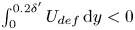 $\int_0^{0.2\delta ^{\prime}} {{U_{def}}\,\textrm{d}y} < 0$ and
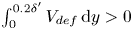 $\int_0^{0.2\delta ^{\prime}} {{V_{def}}\,\textrm{d}y} > 0$, whereas E 2 occurs when
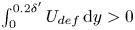 $\int_0^{0.2\delta ^{\prime}} {{U_{def}}\,\textrm{d}y} > 0$ and
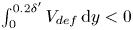 $\int_0^{0.2\delta ^{\prime}} {{V_{def}}\,\textrm{d}y} < 0$. The probabilities of occurrences of E 1 and E 2 were verified and found to be similar for both developed and the developing flow. In both cases, the number of instances corresponding to E 1 and E 2 combined, covers 65 %–70 % of the total number of snapshots. Similar to the analysis presented in § 7.1, the traditional pointwise quadrant analysis is carried out on the instances that belong to E 1 (i.e. estimation of
 ${\overline {u^{\prime}v^{\prime}} _{Q2}}{|_{{E_1}}}$ and
 ${\overline {u^{\prime}v^{\prime}} _{Q4}}{|_{{E_1}}}$) and then on the instances corresponding to E 2 (i.e. estimation of
 ${\overline {u^{\prime}v^{\prime}} _{Q2}}{|_{{E_2}}}$ and
 ${\overline {u^{\prime}v^{\prime}} _{Q4}}{|_{{E_2}}}$). This can be interpretated as a conditional averaging of the instances based on the type of large-scale quadrant events in the logarithmic layer. It is also to be noticed here that only ejections and sweeps are considered for the quadrant analysis since they are the major contributors to shear generation. The quantity
 $- {\overline {u^{\prime}v^{\prime}} _{Qi}}{|_{{E_j}}}$ is estimated by conditional averaging of the shear stress using the following equation:
 \begin{equation}{\overline {u^{\prime}v^{\prime}} _{Qi}}{|_E} = \frac{1}{{{n_E}L^{\prime}\; }}\mathop \sum \limits_1^{{n_E}} \mathop \sum \limits_1^{L^{\prime}} {[u^{\prime}(x,y,t)v^{\prime}(x,y,t)]_{Qi}}\quad \textrm{for}\;i = 2\;\textrm{or}\;4,\end{equation}
where  ${n_E}$ is the number of instances corresponding to a specific event E (E 1 or E 2). The magnitude of
 $- \; {\overline {u^{\prime}v^{\prime}} _{Qi}}{|_E}$ can be interpreted as average shear contribution of all instances that belong to a specific event E and contributes towards Qj. The ratio of shear stress contribution
 $({R_{Q2/Q4}})$ from Q2 and Q4 for a specific event E can be calculated as
 $- {\overline {u^{\prime}v^{\prime}} _{Q2}}{|_E}/{-} {\overline {u^{\prime}v^{\prime}} _{Q4}}{|_E}$ and presented for the developed (figure 15a) and the developing (figure 15b) flow. The solid line corresponding to
 ${R_{Q2/Q4}} = 1$ represents the similar contribution from ejections and sweeps. The dashed line in figures 15(a) and 15(b) separates the logarithmic layer from the defect flow region. Within the logarithmic layer, the pointwise quadrant analysis corresponds well with the identification of large-scale fluid motions based on the velocity deficits. In this region,
 ${R_{Q2/Q4}}$ is greater than one (domination of ejections) for large-scale Q2 events and less than one (domination of sweeps) for large-scale Q4 events. While the distributions of
 ${R_{Q2/Q4}}$ are compared between the developed and developing flow, it is seen that the event E 2 appears to be similar in trend, whereas maximum difference in shear contribution can be found for E 1. Figure 15(b) shows the magnitude of
 ${R_{Q2/Q4}}$ for the developing flow oscillate around one in the region
 $y/\delta ^{\prime} \ge 0.3$ which suggests a balance between the shear generation from ejections and sweeps. But in case of fully developed flow (figure 15a), the magnitude of
 ${R_{Q2/Q4}}$ is much lower than one throughout the domain above the logarithmic layer, which indicates a significant domination of sweeps over ejections. It can be concluded from figure 15 that the shear contribution from the sweeps (as seen over the instances that belong to near-wall ejection events, E 1) is comparatively more prominent in case of fully developed flow.
Distributions of conditionally averaged (based on large-scale ejection events, E 1 or large-scale sweep events, E 2) ratio of shear stress contribution from Q2 and Q4 events for (a) the fully developed flow (T1&T3 at H = 0.170 m) and (b) the developing flow (T0 at H = 0.170 m). The dashed line represents the edge of the logarithmic layer. Every fifth point is shown for clarity.

Further, the distributions of  $- {\overline {u^{\prime}v^{\prime}} _{Q2}}{|_{{E_1}}}$,
 $- {\overline {u^{\prime}v^{\prime}} _{Q4}}{|_{{E_1}}}$,
 $- {\overline {u^{\prime}v^{\prime}} _{Q2}}{|_{{E_2}}}$and
 $- {\overline {u^{\prime}v^{\prime}} _{Q4}}{|_{{E_2}}}$ are presented in figure 16 for both the developed (T1&T3 at H = 0.170 m) and the developing (T0 at H = 0.170 m) flow. These parameters are already used in figure 15 to calculate
 ${R_{Q2/Q4}}$, but are presented separately in figure 16 to depict the variation in the shear distribution. One can recall that the large-scale events are identified based on the velocity deficits in the logarithmic layer which is only used for grouping of the instances. In the present context, there are two groups of instances (E 1 and E 2) and the traditional pointwise quadrant analysis is carried out on each of these groups separately. Importantly, the pointwise quadrant analysis uses the velocity fluctuations, and it is a different concept from the method of identifying large-scale quadrant events. In the logarithmic layer
 $(y/\delta ^{\prime} \le 0.2)$, the large-scale Q2 events can contribute to all four quadrants (based on the pointwise quadrant analysis), however, the contribution to second quadrant can be expected to be dominant over other quadrants as seen in figure 15. The same concept is also valid for large-scale Q4 events. For the ease of the discussion, the significant shear generation in the logarithmic region (contribution to Q2 by large-scale Q2 events,
 $- {\overline {u^{\prime}v^{\prime}} _{Q2}}{|_{{E_1}}}$ and contribution to Q4 by large-scale Q4 events,
 $- {\overline {u^{\prime}v^{\prime}} _{Q4}}{|_{{E_2}}}$) is denoted as direct shear generation, whereas, the contribution to Q4 by large-scale Q2 events
 $( - {\overline {u^{\prime}v^{\prime}} _{Q4}}{|_{{E_1}}})$ and contribution to Q2 by large-scale Q4 events,
 $( - {\overline {u^{\prime}v^{\prime}} _{Q2}}{|_{{E_2}}})$ are named as cross-shear generation.
The distribution of conditionally averaged (based on the large-scale Q2 events defined as  ${E_1}$ and the large-scale Q4 events defined as
 ${E_2}$ in the logarithmic layer) shear stress contribution (a)
 $- {\overline {u^{\prime}v^{\prime}} _{Q2}}{|_{{E_1}}}$, (b)
 $- {\overline {u^{\prime}v^{\prime}} _{Q4}}{|_{{E_1}}}$, (c)
 $- {\overline {u^{\prime}v^{\prime}} _{Q2}}{|_{{E_2}}}$and (d)
 $- {\overline {u^{\prime}v^{\prime}} _{Q4}}{|_{{E_2}}}$) for the fully developed flow (T1&T3 at H = 0.170 m) the developing flow (T0 at H = 0.170 m). The subscript Qi indicates the contribution in ejection and sweep events for i = 2 and 4, respectively. Every fifth point is shown for clarity.

The distributions of direct and cross-shear generation show a contrast in the flow characteristics of a developing and a developed flow. If the direct shear generations in the developed and the developing flow are compared, ejections in the logarithmic layer are found to be the major contributor in fully developed state (figure 16a), whereas figure 16(d) shows that sweeps dominate in generating direct shear stress in the logarithmic layer of the developing flow. Also in figure 16(a,d), a significant shear contribution is found to be restricted to the region adjacent to the bed (i.e.  $y/\delta ^{\prime} \le 0.3$ for
 $- {\overline {u^{\prime}v^{\prime}} _{Q2}}{|_{{E_1}}}$ and
 $y/\delta ^{\prime} \le 0.4$ for
 $- {\overline {u^{\prime}v^{\prime}} _{Q4}}{|_{{E_2}}}$) in the case of fully developed flow, whereas it is distributed over a larger depth in the developing flow (i.e.
 $y/\delta ^{\prime} \le 0.7$ for
 $- {\overline {u^{\prime}v^{\prime}} _{Q2}}{|_{{E_1}}}$ and
 $y/\delta ^{\prime} \le 0.6$ for
 $- {\overline {u^{\prime}v^{\prime}} _{Q4}}{|_{{E_2}}}$). This is likely because of the scale effect of the normalization which helps to depict the constraint provided by the free surface based on their relative location of the boundary layer edge with respect to the total depth of flow. In contrast to the direct shear generation, the cross-shear generations are the major contributors to the shear generation away from the bed and thus control the majority of the quadrant events in the defect flow region. Interestingly, the bed-normal distributions of
 $- {\overline {u^{\prime}v^{\prime}} _{Q2}}{|_{{E_2}}}$ in figure 16(c) are similar in magnitude for both developed and developing flow, indicating a similar contribution to ejections by E 2. However, the ejected fluid parcels in the developing flow can move upward and reach the free-stream flow through momentum exchange between the boundary layer and the outer flow domain. This is not possible in the fully developed flow state and the ejected fluid must be swept away through the surrounding fluid causing higher shear generation due to sweeping events, the evidence of which can be found in the distribution of
 $- {\overline {u^{\prime}v^{\prime}} _{Q4}}{|_{{E_1}}}$ (figure 16b). This shear stress component in fully developed flow is found to be significantly higher than that of developing flow throughout the depth of flow (except very close to the bed). The discussion of figure 16 illustrates the dissimilarities in the shear generation between a developing and a developed open channel flow especially in the defect flow region.
8. Summary and conclusions
The characteristics of the fully developed flow in an open channel are explored using planar PIV measurements. Four different upstream tripping arrangements (T0, T1, T1&T2, T1&T3) are used at two channel aspect ratios, keeping the flow Reynolds number the same. T2 and T3 are additional trips that are used along with a standard trip T1 to stimulate the fully developed flow at aspect ratios of nine and seven, respectively. In fully developed open channel flows, the free-stream region is absent and the flow in the defect layer is influenced by the presence of the free surface. Although free surface velocity or the maximum velocity has been widely used as the equivalent free-stream velocity, uncertainty caused by the free surface perturbations is reasonably high, thus causing inaccuracy in the calculation of boundary layer thickness as compared with a standard TBL. A validation of the ‘log law’ and ‘velocity defect law’ may not be sufficient to identify a fully developed state. Therefore, a revised boundary layer thickness (δ′) based on the turbulence characteristics and higher-order moments is used in the present research since this definition is more reliable than the classical definition of boundary layer thickness based on the wall-normal position of 0.99U∞. T1&T2 is the fully developed state at an aspect ratio of nine (H = 0.135 m) while T1&T3 is the comparable flow at an aspect ratio of seven (H = 0.170 m) in this study. The bed-normal distribution of mean velocity, Reynolds stresses and higher-order turbulence of the two fully developed test cases are evaluated to check and validate for similarity. This ensures that δ′ is the more reliable and acceptable choice of the boundary layer thickness in open channel flow studies.
Once the fully developed open channel flow is achieved, the characteristics of the state of the flow are explored by identifying the zones of uniform momentum. The number of momentum zones in each instance is determined by the peaks in the PDF diagram, which is created by using the velocity data below the TNTI. The position of the TNTI is estimated using the method of Chauhan et al. (Reference Chauhan, Philip and Marusic2014a,Reference Chauhan, Philip, de Silva, Hutchins and Marusicb) with some modifications to suit open channel flow. The PDFs of U/U∞ show a maximum of six peaks for a bin size of 0.5Uτ but only the instances with 2 ≤ NUMZ ≤ 4 are considered for the momentum zone analysis based on a cutoff probability density. The characterization of momentum zones reveals the existence of large-scale Q2 events in the logarithmic layer for the higher number of momentum zones and large-scale Q4 events for a lower number of momentum zones, which is substantiated by the distributions of the velocity deficit. In fully developed state, the characteristics of large-scale fluid motion above the logarithmic layer are opposite i.e. large-scale Q2 events are present for lower number of momentum zones and large-scale Q4 events can be found when number of momentum zones is higher. The conditional averaging of RQ 2/Q4 based on the value of NUMZ shows a vertical variability in the flow characteristics in the fully developed state which is not present in the developing flow. Finally, large-scale ejections and sweep motions and the pointwise quadrant analysis are used simultaneously to demonstrate important differences between the developing and the developed flow condition. In the defect flow region, the sweeping events for the near-wall ejection events, E 1 in the fully developed flow have higher shear generation compared with the developing flow due to the influence of the free surface.
In fully developed flow, the boundary layer thickness is of the order of the total depth of the flow and this restriction causes changes in the flow characteristics. Although the alteration of flow properties cannot be depicted in the time-averaged statistics, present results clearly point to the need to ensure the verification of a fully developed state using some of the procedures indicated herein. In the case of developing open channel flow, the effect of the free surface may vary significantly depending on the relative thickness of boundary layer compared with the depth of the flow. Therefore, it is mandatory to use adequate tripping and stimulation of the fully developed state in any open channel flow study in order maintain the universality of the acquired data.
Declaration of interests
The authors report no conflict of interest.
Appendix A. Dependence of UMZ analysis on threshold kinetic energy deficit and streamwise extent of FOV
In this appendix, we explore the sensitivity and dependency of UMZ analysis to the assigned values of Kth and L +. With a variation in the magnitude of Kth, the position of the TNTI varies and a region of flow may be included in or excluded from the analysis. Similarly, the number of velocity vectors in each instance varies when a different extent of the FOV is chosen in the UMZ analysis. If there is a significant streamwise variation in the flow properties, the number of momentum zones corresponding to each instance may vary significantly with the change in L +. The average number of peaks  $({\bar{N}_{peaks}})$ was estimated for a range of values of Kth (0.7 ≤ Kth ≤ 0.9) and L +(1250 ≤ L + ≤ 2250) for test cases T0 and T1&T3 at H = 0.170 m and no significant deviation is noticed (figure 17) for the current experimental data. Therefore, our current choices of Kth and L + can be safely used without losing generality and changing these choices will not alter the current findings.
Variation of  ${\bar{N}_{peaks}}$ with the change in (a) threshold kinetic energy deficit
 $({K_{th}})$ and (b) length of FOV (L +).

Appendix B. Dependence of UMZ analysis on the bin size
One of the crucial parameters in the momentum zone analysis is the bin size used to generate the PDFs of the streamwise velocities. The number of modal velocities (i.e. the number of momentum zones) for a specific instance will largely depend on the bin size. Since the flow properties are analysed based on the conditional averaging of the instances corresponding to a specific value of NUMZ, it is necessary to ensure that our concluding remarks do not depend on the selection of the bin size (0.5Uτ). Therefore, the momentum zone analysis was carried out with two alternative bin sizes: (i) 0.25Uτ and (ii) 0.75Uτ to check the dependence of UMZ analysis on the bin size. The corresponding PDFs for the bin sizes of 0.25Uτ and 0.75Uτ are presented for the fully developed state and the developing flow (figure 18a,d) and a similar distribution is noticed in both test cases. As a representative flow variable, the bed-normal distributions of RQ 2/Q4 are shown, which are evaluated by conditional averaging of the instances in a range of 3 ≤ NUMZ ≤ 7 (figure 18b,c) and 2 ≤ NUMZ ≤ 3 (figure 18e,f) for the bin sizes of 0.25Uτ and 0.75Uτ, respectively. In case of fully developed flow, the peak magnitude of RQ 2/Q4 moves from y/δ′ ≈ 0.6 to y/δ′ ≈ 0.15 with an increment of NUMZ (figure 18b,e). On the other hand, the peak magnitude of RQ 2/Q4 is located near y/δ′ ≈ 0.7 (figure 18c,f) in the developing flow and does not vary with a change in the number of momentum zones. This follows a similar trend to what was seen earlier with the bin size of 0.5Uτ in § 6.4, proving our findings to be independent of the bin size. A variation in bin size can change the range of NUMZ (or  ${\bar{N}_{peaks}}$) but the comparison between overall flow properties corresponding to higher and lower numbers of momentum zones will be still the same. There may be a possibility of inconsistency in some specific instances, but the impact of this can be nullified when averaging over a large number of datasets.
PDF of NUMZ corresponding to bin size (a) 0.25Uτ and (d) 0.75Uτ for the fully developed flow (T1&T3 at H = 0.170 m) and the developing (T0 at H = 0.170 m). Corresponding bed-normal distribution of  ${R_{Q2/Q4}}$ for bin size 0.25Uτ and 0.75Uτ for (b,e) the fully developed flow and (c,f) the developing flow. In (b,c,e,f), every third point is shown for clarity.