


What’s in a letter like W? A great deal, it turns out, when it comes to modeling spatial dependence. W, the connectivity matrixFootnote 1 that links observations with each other, by definition determines which observations spatially depend on each other—and to what degree they do so. This matrix is often specified according to convenience and spatial econometric modeling conventions rather than based on expectations derived from theory.
In this article we show that for reliable causal inferences about spatial dependence, five aspectsFootnote 2 of the specification of W are crucial and ought to be theoretically justified.Footnote 3 First, the choice of connectivity variable entering W needs to capture the causal mechanism through which spatial dependence works. Second, W determines whether total exposure to spatial dependence is specified as homogenous or heterogeneous. Third, the specification of W needs to capture the relative relevance of each of the sender subjects from whom spatial dependence emanates. In other words, W should specify how important each sender of a spatial stimulus is for each recipient. This may include distinguishing between relevant and irrelevant potential senders. Fourth, in W researchers specify the dimensionality of spatial dependence: whether there is a unique causal channel or multiple ones and, if the latter, whether these are independent of each other, substitutes for one another or conditional on each other. Lastly, the modeling of W determines the directionality of the spatial effect. Subjects can experience a spatial stimulus from senders that is exclusively positive, exclusively negative or positive from some senders, but negative from others.
All theories of spatial dependence need to address these five aspects of W specification. Yet, common practice uncritically follows modeling conventions instead of basing specification choices on theoretical considerations. First, applied researchers often use proxies for the true causal mechanism of connectivity, such as geographical proximity or contiguity. However, spatial effects are caused by transactions, contact, or interactions between the sources and recipients of spatial stimulus. As with all proxies, proximity and contiguity may be useful shortcuts if the true connectivity variable is difficult or impossible to measure, and if the true connectivity variable is highly correlated with proximity. However, since in many cases the true interactions can be observed, there is no reason to use proxies.
Second, row-standardizing W imposes the assumption of homogenous total exposure to spatial stimulus, which flatly contradicts most theories of spatial dependence (Neumayer and Plümper Reference Neumayer and Plümper2012). It achieves this by imposing the restriction that if one subject has fewer ties to other subjects, then each tie is assumed to be more important, which again may run counter to theoretical predictions. Therefore, outside the case in which it is theoretically justified, W should not be row-standardized. There exist alternatives that offer similarly convenient statistical properties without imposing the assumption of homogenous total exposure, and without changing the relative relevance of senders across recipients (see the Exposure section below).
Third, the scaling of the connectivity variable that enters into W does not necessarily match the relative relevance of the senders of spatial stimulus for recipients. It cannot be taken for granted that the measurement scale of connectivity variables accurately approximates the scaling of true connectivity between the senders and recipients of spatial effects.Footnote 4 Scholars typically either employ connectivity variables in their original measurement scale or transform the scale in a rather arbitrary way (for example, by taking the logarithm), whereas they should carefully consider which connectivity variable transformation, if any, is needed to capture the relative relevance of the sources of spatial effects.
Fourth, applied researchers also often neglect the dimensionality of spatial dependence by either assuming there is a unique causal mechanism or insufficiently grasping the challenges posed by multi-dimensionality. The assumption of uni-dimensionality may be appropriate in fields such as epidemiology, in which a spatial effect may depend on a unique type of contact as a causal mechanism. However, other fields, including theories of spatial policy dependence, are usually not characterized by simple, uni-dimensional connectivities.
Fifth, applied researchers nearly always assume that spatial effects are uni-directional. Subjects are either assumed to follow others—as in the international tax competition literature, in which countries are assumed to lower their corporate tax rates in response to others lowering theirs (Plümper, Troeger and Winner Reference Plümper, Troeger and Winner2009)—or, less commonly, to be negatively influenced by others, for example in Franzese and Hays’ (Reference Franzese and Hays2006) analysis of spending on active labor market policies in which higher spending by contiguous neighbors results in lower spending by the recipients of this spatial stimulus. However, neither of these types of studies allows a positive spatial stimulus from some senders and a negative stimulus from others. In many fields of research, this specification is a conceptual mistake. For example, governments can be eager to adopt the policies of other governments with a similar political orientation, but may actively avoid the policies of governments with opposing political orientations. Thus spatial dependence can be positive for some sources of spatial stimulus, but negative for others.
This article explains how W should be specified. We start by demonstrating the restrictive specification choices imposed by the standard modeling conventions for W. We then discuss each of the five crucial aspects for modeling W in detail. Specification choices should follow theory rather than convention. Theory also trumps data mining, which is why we find attempts that estimate W based on the data to be unappealing (see, for example, Aldstadt and Getis Reference Aldstadt and Getis2006; Beenstock and Felsenstein Reference Beenstock and Felsenstein2012; Lam and Souza Reference Lam and Souza2013). Yet we appreciate that theories will typically be under-specified, providing some (but insufficiently detailed) guidance. Theoretically derived specification dominates modeling conventions, but when theories are under-specified, researchers can adopt the flexible specifications we propose here to test the robustness of their inferences to equally plausible model specification choices.
Modeling Conventions For The Specification Of W
In this section, we show how the standard modeling conventions for specifying W impose certain assumptions on four of the five crucial specification choices that affect inferences in the analysis of spatial dependence. The use of geographical proximity as a connectivity variable functioning as a proxy for the causal mechanism of spatial dependence is not part of standard modeling conventions as such, but is nevertheless a fairly widespread practice.
Anselin, Le Gallo and Jayet (Reference Anselin, Le Gallo and Jayet2008, 627) define spatial dependence as being present “whenever correlation across cross-sectional units is non-zero, and the pattern of non-zero correlations follows a certain spatial ordering.” Yet such a spatially ordered pattern does not imply spatial dependence in a strict sense. It can also emerge when the similarity of units follows a spatially ordered pattern. Thus spatial dependence should be distinguished from spatial clustering—for both econometric and theoretical reasons.
If we make this distinction, then the analysis of spatial dependence proper is confined to spatial lag and spatial-x models, while spatial error models may be used to correct for spatial clustering. Spatial lag or spatial autoregressive models model spatial dependence in the dependent variable, spatial-x models in one or more explanatory variables and spatial error models in the error term. For expositional simplicity, we will focus on spatial lag models, the most common model of spatial dependence, but all of our arguments apply to the other types of models of spatial dependence as well as combinations of these.Footnote 5
Using a scalar notation, the standard modeling convention for specifying W in a spatial lag model based on a monadicFootnote 6 cross-sectional time-series or panelFootnote 7 dataset is as follows:
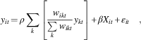 $$y_{{it}} \,{\rm =}\,\rho \mathop{\sum}\limits_k {\left[ {{{w_{ikt} } \over {\mathop{\sum}\limits_k {w_{{ikt}} } }}y_{kt} } \right]} {\rm {\plus}}\beta X_{{it}} {\rm {\plus}}{\varepsilon}_{{it}}\quad ,$$
where  $i=1,2,..,N$
,
 $t=1,2,..,T$
,
 $k=1,2,..N$
. Notation is standard so that y it is the value of the dependent variable in unit i at time t, and
 $$\mathop{\sum}\limits_k {\left[ {{{w_{ikt} } \over {\mathop{\sum}\limits_k {w_{{ikt}} } }}y_{kt} } \right]} ,$$
is a row-standardized spatial lag variable, X it is a vector of unit-specific variables influencing y it, and  ${e}_{{it}} $
is an identically and independently distributed (i.i.d.) error process.Footnote 8
The spatial autoregression parameter ρ represents the estimated degree of spatial dependence. The spatial effect Variable 2 consists of the product of two elements. The first element is the  $N \cdot N \cdot T$
block-diagonal row-standardized spatial weighting matrix W, which measures the relative connectivity between N number of units i (call them recipients of spatial stimulus) and N number of units k (call them senders of spatial stimulus) in T number of time periods in the off-diagonal cells of the matrix as represented by the connectivity variable w ikt, which takes on strictly non-negative values only (Anselin 2002, 258).
This standard modeling convention implicitly imposes assumptions about four of the five aspects of the specification of W that, we argue, need to be derived from theory instead of convention. By row-standardizing W—each w ikt is divided by  $$\mathop{\sum}\nolimits_k {w_{{ikt}} } $$
, the row sum of connectivities—the assumption of homogenous total exposure to spatial stimulus is imposed across all recipient subjects. The relative relevance of the senders of spatial stimulus is represented by different values of w ikt for different dyads of recipient i and sender k. Yet the relative relevance of senders across recipients is transformed by row-standardizing W in ill-understood and often theoretically unappealing ways. Also, transformations of the connectivity variables severely impact the relative relevance of senders for each recipient (see the Exposure section below).
At least implicitly, Equation 1 assumes that spatial dependence is uni-dimensional. If researchers deviate from the assumptions underlying Specification 1 and employ several connectivity variables, these are typically employed in separate spatial effect variables with no theoretical justification for the ensuing implicit assumption that the multiple dimensions are independent of each other, rather than substitutes for (or conditional on) each other.
Finally, by requiring w ikt to take on strictly non-negative values only, and by estimating one coefficient for one single spatial lag variable, Specification 1 assumes that spatial dependence is uni-directional. The implicit assumption of uni-directionality seems strongly embedded in spatial econometric applications in political science. In fact, outside the field of spatial dependence in arms races and military expenditures, we know of only one analysis that allows for bi-directional spatial effects (Brooks and Kurtz Reference Brooks and Kurtz2012).Footnote 9
Specification Choices From A Generalized Theory Of Spatial Dependence
Having shown which assumptions standard modeling conventions impose on the specification choices of W, we now discuss in detail each of the five modeling aspects that any theory of spatial dependence needs to address. As will become clear, modeling conventions often conflict with appropriate specification choices derived from theories of spatial dependence.
The Causal Mechanism of Spatial Dependence
Theories of spatial dependence require a causal mechanism by which outcomes of sender subjects k—behavior, policies, events or whatever else is spatially dependent—affect recipient subjects i. This causal mechanism must be captured by the connectivity variable w ikt and its specification in W.
Traditionally, spatial analysts, including those in political science, have employed measures of geographical proximity as connectivity variables. A search of articles published in political science journals over the last four years suggests that many applications still do (for example, Leeson and Dean Reference Leeson and Dean2009; Flores Reference Flores2011; De Francesco Reference De Francesco2012; Faber and Gerritse Reference Faber and Gerritse2012), even if some applications now explicitly include non-geographical connectivity variables thought to capture the causal mechanism of spatial dependence among jurisdictions (for example, Cao and Prakash Reference Cao and Prakash2010; Linos Reference Linos2011; Baccini and Dür Reference Baccini and Dür2012). Beck, Gleditsch and Beardsley (Reference Beck, Gleditsch and Beardsley2006, 42) trace this dominance to the geographic heritage of spatial econometric models: “their primary application has been to incorporate physical notions of space (distance) into political models, and, particularly, to argue that geographically nearby units are linked together (…).” Despite the call by Beck, Gleditsch and Beardsley (Reference Beck, Gleditsch and Beardsley2006), ourselves (Neumayer and Plümper Reference Neumayer and Plümper2012) and others (for example, Zhukov and Stewart Reference Zhukov and Stewart2013) to employ connectivity variables that directly capture the causal mechanism of spatial dependence, contiguity and geographical proximity are still widely used. Spatial econometricians have also been slow in accepting non-geographical connectivity variables in spatial models. Some explicitly favor geographical connectivity variables on the grounds that they are typically not endogenous to the variable being spatially lagged, whereas substantive connectivity variables can be (for example, LeSage and Pace Reference LeSage and Pace2011, 18). While we recognize the need for further research into inferential threats caused by potentially endogenous connectivity variables, we disagree that this suggests that geographical proximity is a good connectivity variable. A misspecified connectivity variable is still misspecified, even if it is “exogenous.”
The reason why employing geographical proximity typically results in misspecification is that geographical proximity is not the causal mechanism that causes spatial dependence. Rather, connectivity is. Space is not only “more than geography” (Beck, Gleditsch and Beardsley Reference Beck, Gleditsch and Beardsley2006); spatial dependence is clearly not caused by geography, proximity and contiguity itself. Rather, it is caused by connectivitiy, i.e. contact in its various forms, transactions, interactions and relations. Employing geographical proximity is thus nothing more than based on the functionalistic assumption that proximity is correlated with contact intensity or contact frequency. Thus atheoretical connectivity variables such as geographical proximity typically cannot provide insights into the true causal mechanism of spatial dependence, and are therefore often inappropriate for testing theories of spatial dependence.
The use of geographical proximity as a connectivity variable threatens the reliability of inferences in spatial models in two major ways. First, the functionalistic logic of using geographical proximity as a substitute for measures of contact is vaguely based on Tobler’s first law of geography, according to which “everything is related to everything else, but near things are more related than distant things” (Tobler Reference Tobler1970, 236). The functional equivalence between proximity, on the one hand, and relation, contact or interaction on the other hand may well hold in many applications. However, in other applications they are truly independent of proximity. More importantly, in many more applications, proximity is only weakly correlated with connectivity. Yet unless proximity is sufficiently highly correlated with relation, contact, transactions or interaction, a spatial analysis that uses proximity as a connectivity variable is likely to result in wrong inferences not merely about the estimated degree of spatial dependence, but even with regards to inferences about the very existence of spatial dependence.
Second, unless geographical proximity is sufficiently highly correlated with connectivity, its use as a connectivity variable poses a particular risk to reliable inferences, because the geographical proximity of two subjects is likely to be correlated with similarity. Thus, as a caveat to Tobler’s first law and very much in his language, we suggest the following second law of geography: Everything resembles everything else, but near things are more similar than distant things. If our second law of geography holds, then geographical proximity between subjects is likely to be correlated with any misspecification of the econometric model (Quah Reference Quah1993). Consider the example of an omitted variable: if the omitted variable is spatially correlated (if close things are more similar), a spatial lag that uses geographic proximity as a connectivity variable is likely to be correlated with the omitted variable, in which case the estimation of the effect of the spatial lag would be biased, and any inferences would be potentially wrong.
For most theories of spatial dependence, geographical proximity is a poor proxy for connectivity. Three broad causal mechanisms can be distinguished (Neumayer and Plümper Reference Neumayer and Plümper2012, 822–7): learning, which is indistinguishable from emulation; externalities, which include competition; and coercion. Closer units are likely, but not certain, to interact more with each other and thus able to learn from each other. Subjects can be physically very close and not learn from each other at all. Learning occurs through observation, interaction and communication (Hall Reference Hall1993; Dolowitz and March Reference Dolowitz and Marsh1996; Gilardi Reference Gilardi2010). Thus ideally, measures of these ties would be directly employed as connectivity variables.
The same holds for externality-based theories of spatial dependence. Direct externalities require the exchange of goods, services, capital, persons or pollutants between senders and recipients, which transmit the externality from the former to the latter. Closer units may be more likely to impose externalities onto other units or impose larger externalities. However, there is no guarantee that proximity is strongly correlated with externalities. This becomes even clearer when we consider indirect externalities transmitted through economic competition (Elkins, Guzman and Simmons Reference Elkins, Guzman and Simmons2006; Cao and Prakash Reference Cao and Prakash2010). Japan and Germany are in many respects close competitors, though the countries are geographically very distant.
Coercion as a causal mechanism of spatial dependence depends on the leverage that senders have over recipients. Geographical proximity is likely to be uncorrelated (or at best weakly correlated) with such leverage. Former colonial masters might have substantial leverage over their ex-colonies that can be located in distant places, for example. Developed country aid donors might have substantial leverage over aid recipients in the developing world, but the extent of their leverage is unlikely to be closely related to geographical proximity.
Exposure
Spatial econometricians find it convenient to “row-standardize” the weighting matrix. It is a convention that is “typically” (Anselin 2002, 257), “commonly” (Franzese and Hays Reference Franzese and Hays2006, 174), “generally” (Darmofal Reference Darmofal2006, 8), or “usually” (Beck, Gleditsch and Beardsley Reference Beck, Gleditsch and Beardsley2006, 28) followed. As we have shown above, row-standardization is a mathematical transformation that divides the observed connection between the subject under observation i and other subjects k by the sum of connections of each i.
While econometrically convenient, the convention of row-standardization often clashes with theories of spatial dependence and their predictions about heterogeneity in the total exposure of subjects to spatial stimulus (Neumayer and Plümper Reference Neumayer and Plümper2012). Row-standardization takes out all level effects from the connectivity matrix—for each recipient i, the sum of connectivities to all sources k equals 1. Row-standardization thus imposes the assumption that total exposure to the spatial stimulus is equal for all units i. It implies that if two different recipients are linked to the same senders, but one has barely any connectivity to senders and the other is strongly connected to them, they will end up with the exact same row-standardized spatial stimulus (same value of the spatial effect variable).Footnote 10 We call this homogeneity of total exposure to spatial stimulus.
Table 1 gives an example. Note that w ik denotes the unstandardized values of the weights, while we use  $w'_{{ik}} $
to mark the row-standardized weights for two units, i 1 and i 2, which receive a spatial stimulus from the same five senders, k 1…k 5. Observe that i 2 has links to k 1…k 5 that are 10 times smaller than those of i 1. However, if we row-standardize W, then the resulting spatial lag variable takes on the same value for both i 1 and i 2. Accordingly, if theories predict that recipient i 2 receives a far weaker spatial stimulus from k 1 to k 5 than i 1 due to its lower overall level of connectivity, then row-standardizing the weighting matrix is clearly not the way to go.
The Homogenous Total Exposure Assumption of Row-Standardization

A second consequence of row-standardization is equally consequential but arguably less known. In order to achieve homogenous total exposure, row-standardization implicitly imposes the atheoretical and often implausible assumption that if one receiver has fewer (more) connections to senders of spatial influence, each sender becomes more (less) important. Table 2 provides a different example.
Adding Further Contacts Reduces the Spatial Weight of Each One

Observe that the number of contacts that i 2 has with k 1 to k 5 is one larger than the number of contacts that i 1 has. As a consequence, the weight of each individual contact in the row-standardized weighting matrix declines from 0.50 for i 1 to 0.33 for i 2. Consider the case of learning theories: row-standardization would be appropriate if (and only if) the learning success of recipients i was independent of the number of senders k but only depended on being a recipient of spatial stimulus at all. If, however, recipients learn more if they are in contact with more senders, then row-standardization leads to a misspecified model.
How plausible is the assumption of homogenous total exposure to spatial stimulus imposed by row-standardizing W? Whether one expects the total exposure to spatial stimulus to be homogenous or heterogeneous across subjects is principally a theoretical question. If theory predicts that total exposure is homogenous, W has to be row-standardized. Yet in the majority of applications, theories of spatial dependence suggest heterogeneous total exposure, which would mean that row-standardizing W misspecifies the theoretical model. For example, any theory of regulatory or policy competition is likely to predict that total exposure to spatial stimulus varies from jurisdiction to jurisdiction (Garrett Reference Garrett1995; Genschel and Plümper Reference Genschel and Plümper1997; Basinger and Hallerberg Reference Basinger and Hallerberg2004; Schmitt Reference Schmitt2011). Thus a globally integrated country like South Korea is much more exposed to the imperatives of regulatory competition than an economically closed one such as North Korea. Similarly, in dyadic analysis, total exposure is likely to vary from country dyad to country dyad—see, for example, Baccini and Dür (Reference Baccini and Dür2012), who explicitly decide against row-standardizing W in their analysis of spatial dependence in preferential trade agreement formation. In Neumayer and Plümper (Reference Neumayer and Plümper2012), we make a detailed case for heterogeneous total exposure for all causal mechanisms of spatial dependence.
In Plümper and Neumayer (Reference Plümper and Neumayer2010) we demonstrated that row-standardization is not inferentially neutral and will, unless theoretically justified, result in misspecified spatial models. Few spatial econometricians seem to recognize this. Kelejian and Prucha (Reference Kelejian and Prucha2010) are a notable and laudable exception. They state:
[I]n row-normalizing a matrix one does not use a single normalization factor, but rather a different factor for the elements of each row. Therefore, in general, there exists no corresponding re-scaling factor for the autoregressive parameter that would lead to a specification that is equivalent to that corresponding to the un-normalized weight matrix. Consequently, unless theoretical issues suggest a row-normalized weight matrix, this approach will in general lead to a misspecified model (Kelejian and Prucha Reference Kelejian and Prucha2010, 56)
There is no excuse for row-standardization based on statistical convenience either, since convenient properties such as matrix nonsingularity can instead be achieved by a min-max-normalized matrix: each cell is divided by m=min{max(r i), max(c i)}, where max(r i) is the largest row sum of W and max(c i) the largest column sum of W (Kelejian and Prucha Reference Kelejian and Prucha2010, 56; Drukker et al. Reference Drukker, Peng, Prucha and Raciborski2013, 251). By dividing the matrix W by a single scalar rather than the row sum for each observation i, which differs across all spatial effect recipients i, min-max normalization does not impose the assumption of homogenous total exposure and therefore does not change the relative relevance of senders across recipients. Alternatively, as Neumayer and Plümper (Reference Neumayer and Plümper2012) demonstrate, one can test whether a row-standardized spatial effect becomes stronger as the total exposure to spatial stimuli increases across subjects. This is possible with a model in which a row-standardized spatial effect variable is interacted with a measure of exposure z it:Footnote 11
 $$y_{{it}} =\rho _{1} \mathop{\sum}\limits_k {\left[ {{{w_{ikt} } \over {\mathop{\sum}\limits_k {w_{{ikt}} } }}y_{kt} } \right]} {\plus}\rho _{2} \mathop{\sum}\limits_k {\left[ {{{w_{ikt} } \over {\mathop{\sum}\limits_k {w_{{ikt}} } }}y_{kt} } \right]} \cdot z_{{it}} {\plus}\rho _{3} z_{{it}} {\plus}\beta X_{{it}} {\plus}{\varepsilon}_{{it}} \,\,\,\,\,\,.$$
Evidence for heterogeneous total exposure would follow if the effect of the row-standardized spatial lag variable were conditioned by the measure of exposure. This model specification leaves open the decision of whether heterogeneous or homogenous total exposure is appropriate to the data.
In sum, it is important to understand that row-standardization is not theoretically neutral—it is not a transformation that leaves the estimates unchanged, but rather one that exerts a potentially strong influence on estimates and inferences. Researchers cannot hide behind econometric conventions. They have to derive a prediction about the total exposure to spatial stimulus from their theory. In most cases, row-standardization conflicts with theory and there is no excuse based on statistical convenience for it. This should bring the discussion about row-standardization to an effective halt: it typically results in misspecification and should therefore be abandoned.
Relative Relevance
Determining the relative relevance of sources is a broader specification issue, which is not only influenced by whether or not to row-standardize W. Its starting point is considering whether any of the potentially sending subjects k are entirely irrelevant for recipient subject i under observation. If so, this results in a value of zero for the cell in W representing the link between subject i and subject k.Footnote 12
Assuming that spatial dependence emanates from only one group of observations (a subset of k) can make sense—for example, in epidemiology, where the transmission of a disease is impossible unless two units have had direct prior physical contact. Neumayer, Plümper and Epifanio (Reference Neumayer, Plümper and Epifanio2014) provide an example from political science by arguing that the implementation of counterterrorist regulations in developed Western democracies is solely influenced by the implementation of such policies in countries with a similar threat level. If this holds, then the spatial effect emanating from unlinked units is zero and the model is correctly specified. If the theory is correct, and there is no spatial effect from units with which there was no previous physical contact, then the coefficient of the spatial effect variable employing a dummy variable coded 1 for units with which no prior physical contact was had will be zero (assuming the estimation model is otherwise correctly specified).
More generally, however, there will be some uncertainty over whether the theory is correct or whether the group that is irrelevant for spatial dependence has been established without non-negligible measurement error. Therefore, if researchers are uncertain whether the spatial effect of the group deemed to be irrelevant is actually zero, they can estimate the following specification (we show all specifications without row-standardization):
 $$y_{{it}} =\rho ^{1} \mathop{\sum}\limits_k {{w^{1} _{{ikt}} y}_{kt} } {\plus}\rho ^{2} \mathop{\sum}\limits_k {w^{2} _{{ikt}} y_{kt} } {\plus}\beta X_{{it}} {\plus}{\varepsilon}_{{it}} \,\,\,\,\,\,,$$
where 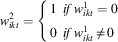 $w^{2} _{{ikt}} =\left\{ \matrix{ 1\,\;if\,w^{1} _{{ikt}} =0 \hfill \cr 0\,\;if\,w^{1} _{{ikt}} \,\ne\,0 \hfill \cr} \right.$
. Where
 $$w^{1} _{{ikt}} $$
is a dichotomous variable, this would simplify to
 $$w^{2} _{{ikt}} =(1{\minus}w^{1} _{{ikt}} )$$
.Footnote 13 In principle, it is not a bad idea to estimate Equation 4 even in cases in which researchers are convinced that the group of subjects, for which
 $$w^{1} _{{ikt}} =0$$
and therefore
 $$w^{2} _{{ikt}} =1$$
, exerts no spatial effect. Rather than imposing this constraint on the model specification, it can be better to test this hypothesis and estimate Equation 4.
Going beyond the specification choice that determines which potential sending subjects are entirely irrelevant, the second crucial specification that determines relative relevance is specifying the relative weight assigned to each relevant sending subject k for each receiving subject i under observation. The relative weight of sending subjects k is principally determined by the range and scale of the connectivity variable, to which we turn our attention now.
Connectivity variables are measured in specific units—for example, trade in USD or some other currency, or social contact by the number of visits. Any transformation of connectivity variables that leaves the distribution of the variable intact—in the sense that the ratio of all variable values to each other remains the same—is inferentially neutral. Multiplication by a constant factor is an example of such an inferentially neutral transformation. It thus does not matter whether a connectivity variable is measured in, say, USD or thousands or millions of USD or is held in euros or yen instead.
Other transformations change the relative weight of sending subjects, however. Thus taking the log, the square root or raising the connectivity variable to some power all affect the distribution of weights and thereby the relative relevance of sending subjects k. Most importantly, adding or subtracting a constant is not an inferentially neutral transformation either. This latter aspect reveals how the connectivity variable differs from variables in the estimation model: a constant added to or subtracted from the connectivity variable cannot be absorbed in the intercept. That adding a constant is not inferentially neutral also has consequences for the use of categorical connectivity variables, which cannot be employed as if they were cardinal.Footnote 14 Instead, separate spatial effect variables need to be created based on dummy variables as connectivity variables for each category. There is one exception to this: if, for relevant senders, the average value (row-standardized W) or sum (not row-standardized W) of the variable to be spatially lagged is the same in one category of source units k as in another category of units k. In this case, one should merge the two categories into one.
To illustrate how transformations other than multiplication by a constant factor change the relative relevance of sending subjects, consider proximity among countries, here defined as 1/distance, as a connectivity variable. We choose proximity for illustrative purposes only, notwithstanding our argument that geographical proximity should best be avoided as a connectivity variable since it typically fails to capture the underlying causal mechanism (see the Exposure section above). The closest countries are neighboring each other and thus have a distance of 0 or—if measuring the distance between capitals—10.5 kilometers (Kinshasa in the Democratic Republic of Congo and Brazzaville in the Republic of Congo). The two countries that are furthest apart are Mali and Samoa, with just over 19,900 kilometers between them. The range of the connectivity variable 1/distance varies by a factor of 190. In other words: using 1/distance as a proxy for the intensity of relations, the influence of the two Congos on each other would be assumed to be 190 times bigger than the influence of Mali and Samoa on each other. This assumption changes drastically if we do what researchers using distance often do: take the natural log of distance. If we do this, we assume that the influence of the two Congos on each other is only 4.21 times stronger than the influence of Mali on Samoa, and vice versa.
However, variable transformation is not the only way in which connectivity variables are rescaled. As stated in the previous sub-section, row-standardization also results in changes to relative weights. After row-standardization, the country dyad that is furthest apart has changed to Kiribati as the receiver and the Republic of Congo as the sender of spatial stimulus (the two Congos remain the dyads closest to each other), and the ratio of largest to smallest distance has increased to a factor of 1,676 for 1/distance as a connectivity variable. The row-standardization thus not only attributes the smallest weight to a different dyad—the dyad of maximum distance to any other country (which happens to be the Republic of Congo) to Kiribati as the recipient, which is the most isolated country in the world in the sense that it is, on average, the furthest apart from other countries—it has also dramatically decreased the weight that far-away countries have for such isolated countries. Not surprisingly, for 1/(ln distance) as a connectivity variable, the ratio between the highest to lowest weight increases only a little, to a factor of 4.34. Taking the log massively contracts the range of distances among countries, such that the distances of relatively isolated countries to other countries translate into proximity weights that are much more similar to those of centrally located countries compared to the row-standardized proximity in levels.
Importantly, row-standardization also breaks the symmetry of weights between two countries of one dyad. Whereas, as already pointed out, Kiribati as recipient and the Republic of Congo as sender takes on the minimum value if 1/distance is row-standardized, the link between the Republic of Congo as recipient and Kiribati as sender is not even in the lowest quartile of row-standardized proximity! The reason is Congo’s relatively central position on the globe, which makes large absolute distances to senders much smaller after row-standardization compared to large absolute distances in isolated recipient countries. This is yet another example of how row-standardization changes the relative relevance of senders across recipients in ill-understood ways.
While both variable transformations and row-standardization thus affect the relative relevance of senders, they do so in very different ways. Variable transformation changes the relative relevance of senders for each recipient, but it leaves the order of weights exactly the same across all recipient-sender dyads. The dyads of least and most proximity, and the rank ordering of all dyads in between these two extremes, will be exactly the same regardless of whether 1/distance or 1/(ln distance) is used. Row-standardization, on the other hand, leaves the relative relevance of senders for each recipient intact (weights are merely divided by a constant factor for each recipient), but it changes the order of weights across recipient–sender dyads and thus changes the relative relevance of senders across recipients.
In Plümper and Neumayer (Reference Plümper and Neumayer2010) we have shown that estimation results (and thus inferences) can be very different for a spatial lag variable that is based on the inverse of distance as opposed to being based on the inverse of logged distance. We have shown the same for row-standardized versus not row-standardized W. Row-standardization and transformations other than multiplication by a constant factor change the distribution of the connectivity variable and thereby the relative weight of senders. Row-standardization does so implicitly and across recipients, whereas power transformations do so explicitly and for each recipient.
Different distributions after a variable has been rescaled either via a transformation or row-standardization can be understood as imposing different functional forms onto the connectivity between senders and recipients. The “correct” functional form for connectivity may exist, but unfortunately it remains unknown and cannot be estimated. Most spatial applications employ the untransformed connectivity variable and row-standardize it. However, there is no a priori reason why the strength of spatial stimulus needs to decay linearly with increasing geographical distance if proximity is one’s connectivity variable. The strength of spatial stimulus could decay as a function of the logarithm of distance, distance squared or distance plus distance squared, and so on.
Depending on one’s theory, a different functional form in accordance with a specific transformation may therefore be theoretically warranted. If one has strong reasons to assume a specific functional form, then one can impose this functional form and transform the connectivity variable accordingly, using the resulting transformed variable as the new connectivity variable in W. Generally speaking, however, theory rarely provides such detailed specification advice.
With under-specified theories, researchers have great leeway in picking a transformation that suits them in terms of finding support for their tested hypothesis, which in turn is one of the reasons why models of spatial dependence have a problematic “anything goes” character. Given this under-specification problem, a semi-parametric approach represents a promising alternative. One divides one’s connectivity variable into several categories, creating separate dummy variables for each. For example, for distance one would create separate dummies for bands of distance (for example, from 0 to 1,000 kilometers, 1,001 to 2,000 kilometers, etc.) and then create separate spatial effect variables, one for each category. This would allow the strength of the spatial stimulus to vary flexibly across the range of the connectivity variable rather than imposing a particular functional form. The approach is semi-parametric, in the sense that no specific functional form is parametrically imposed on the connectivity between units i and k. In general, m categories allow for at most m−1 turning or inflection points in the connectivity between i and k.
Such semi-parametrically operationalized spatial effect variables qualify our verdict in Plümper and Neumayer (Reference Plümper and Neumayer2010, 434) that “the correct operationalization and functional form of connectivity must be known (based on theoretical reasoning) by the researcher.” The semi-parametric approach in fact allows researchers to let the data determine the functional form of connectivity rather than imposing a specific functional form.
Into how many categories should the connectivity variable be grouped, and how should one group observations into distinct categories? Starting with the latter question, for continuous variables one can group observations into categories of equal width or into percentiles. Equal width means grouping observations into categories of equal size in terms of the unit of measurement of the variable, such as equally wide bands of distance (0 to 1,000, 1,001 to 2,000; 2,001 to 3,000 kilometers and so on). Percentiles require creating dummy variables for, say, the 25th percentile, 50th percentile and so on. For count variables and for interval variables that are not strictly continuous or not strictly continuously recorded, splitting the variable’s range into percentiles does not make much sense since observations cannot, unless by chance, be split into value ranges that are equally inhabited by observations. How many categories should researchers build? Not too many: connectivity is unlikely to have many inflection and turning points, and the spatial effect variables created for each category will be correlated with each other, leading to efficiency losses. Hence, 3–5 categories will often suffice, but more categories can be warranted.
The semi-parametric approach is not without problems. Within categories, weights are assumed to be the same, which may not be appropriate. More importantly, the choice of the number of categories (and the thresholds between them) is arbitrary. Therefore, the semi-parametric approach needs to be conducted along with extensive robustness tests that demonstrate the independence of inferences from both arbitrary decisions.
Dimensionality
Connectivity can be multi-dimensional. Sometimes, theory will require multi-dimensional connectivity if several causal mechanisms exist that transmit a spatial stimulus from sources to recipients. Empirically, connectivity can be multi-dimensional even if theory suggests there is a single causal mechanism that cannot be directly measured and is instead approximated by more than one proxy variable.
Multiple dimensions of connectivity can represent links between i and k that are independent of each other, substitutive for each other or conditional on each other. Multiple dimensions of connectivity that are truly independent of each other—that is, neither substitutive for each other nor conditional on each other—are probably rare, since even different causal mechanisms may not be entirely independent of each other. But where multiple dimensions are approximately independent of each other, they should be modeled by separate spatial effect variables. Only by estimating the coefficients of separate spatial effect variables will one be able to test whether there is evidence for spatial dependence working via a specific causal mechanism and test which of the causal mechanisms is substantively stronger than others. Note, however, that due to the interdependencies among subjects that is inherent to spatial dependence, it is not possible to completely separate out the effect estimates of each of several individual spatial effect variables (Elhorst, Lacombe and Piras Reference Elhorst, Lacombe and Piras2012).
Multiple dimensions of connectivity that are not independent of each other likely exist where one has several connectivity measures that capture the same causal mechanism. Different connectivities can be substitutes for each other, even perfect substitutes. If the latter, one can simply add up the measures of the various connectivity variables. For example, one may employ international visitor flows as connectivity. Unless one has reason to believe that incoming visitors from countries k to country i represented a different causal mechanism or the same causal mechanism, but of different strength, compared to outgoing visitors from country i to countries k, then one can simply add the visitor flows in both directions into one overall variable representing total bilateral visitor contact. As another example, when it comes to the exchange of information, visits of one actor by another, telephone calls, email exchanges, old-fashioned letters and fax messages can all substitute for each other. In reality, the amount of shared information may vary, but as an approximation, the best measure of total interaction may well be a simple sum of all these activities. An example of three connectivity variables—superscripted 1, 2, 3 and assumed to be perfect substitutes for each other—leads to the following specification:
 $$y_{{it}} =\rho \left[ {\mathop{\sum}\limits_k {\left( {w_{{ikt}}^{1} {\plus}w_{{ikt}}^{2} {\plus}w_{{ikt}}^{3} } \right)y_{{kt}} } } \right]{\plus}\beta X_{{it}} {\plus}{\varepsilon}_{{it}} \,\,\,\,\,\,.$$
Yet scholars will often be uncertain whether multiple connectivities are perfect substitutes for each other. Two further options are then available. One is to create three separate spatial effect variables that employ each of these connectivity variables separately. The third option is to create a principal component from the connectivity variables and use the resulting variable as a measure of aggregate connectivity. For our example of three connectivity variables, the second option would lead to
 $$y_{{it}} =\rho ^{1} \mathop{\sum}\limits_k {w_{{ikt}}^{1} y_{{kt}} } {\plus}\rho ^{2} \mathop{\sum}\limits_k {w_{{ikt}}^{2} y_{{kt}} } {\plus}\rho ^{3} \mathop{\sum}\limits_k {w_{{ikt}}^{3} y_{{kt}} } {\plus}\beta X_{{it}} {\plus}{\varepsilon}_{{it}} \,\,\,\,\,\,,$$
whereas the third option would result in
 $$y_{{it}} =\rho \mathop{\sum}\limits_k {\Phi _{{ikt}}^{{}} y_{{kt}} } {\plus}\beta X_{{it}} {\plus}{\varepsilon}_{{it}} \,\,\,\,\,\,,$$
where  $$\Phi _{{ikt}}^{{}} $$
is a principal component of
 $$w_{{ikt}}^{1} $$
,
 $$w_{{ikt}}^{2} $$
and
 $$w_{{ikt}}^{3} $$
.
Specification 6 estimates more parameters and thus imposes the fewest constraints. It also has drawbacks, however. It assumes that the multiple dimensions of connectivity are not conditional on each other, and are thus either independent or substitutive. If this assumption is wrong, then Specification 6 is wrong and should be replaced by one that includes interaction effects among the connectivities—discussed further below. If the assumption is correct, then a comparison of the estimated degrees of spatial dependence in this specification can in principle also indicate whether the three forms of connectivity are perfect substitutes for each other, which can be inferred if the estimated degrees of spatial dependence do not statistically significantly differ from each other. The practical problem, however, is that the spatial effect variables based on each of the separate connectivity variables will be correlated with each other, and potentially strongly so. This can result in substantial efficiency losses and even multicollinearity problems. If such problems are detected, then scholars can move to one of the other options. If the multiple connectivity variables are found to be perfect substitutes for each other, then the first option of adding up the multiple connectivity variables into a single connectivity variable is an attractive one. Note that this specification is not available if the multiple connectivity variables are measured in different units.
So far, we have discussed multi-dimensional connectivity where the multiple dimensions are either independent of each other or substitutive for each other. The multiple dimensions can also be conditional on each other, such that a particular value of connectivity on one individual variable results in a higher overall connectivity value if the other individual connectivity variables take on higher values. Such conditionality can be captured by a multiplicative relationship between two (or more) connectivity variables, which results in the following specification (for notational simplicity we assume only two individual connectivity variables):
 $$y_{{it}} =\rho \mathop{\sum}\limits_k {\left( {w_{{ikt}}^{1} \cdot w_{{ikt}}^{2} } \right)y_{{kt}} } {\plus}\beta X_{{it}} {\plus}{\varepsilon}_{{it}} \,\,\,\,\,\,.$$
An extreme version of Equation 8 is if one of the weights, say  $$w_{{ikt}}^{2} $$
, is a dummy variable, in which case the effect of spatial dependence working via connectivity
 $$w_{{ikt}}^{1} $$
is conditional on
 $w_{{ikt}}^{2} =1$
. Multiplication is not the only way to represent conditional relationships among individual connectivity variables, however. In principle, any combination that is not linearly additive could be used (or some logical operation combining the individual connectivity variables), and the combination could also potentially include higher-order terms of the individual connectivity variables (see Anselin 2002, 259 for some examples).
An alternative way of capturing a conditional relationship among multiple connectivity variables is to create separate spatial effect variables built on each one and then to model a conditional relationship via an interaction effects model, which would result in the following specification:
 $$y_{{it}} =\rho ^{1} \mathop{\sum}\limits_k {w_{{ikt}}^{1} y_{{kt}} } {\plus}\rho ^{2} \mathop{\sum}\limits_k {w_{{ikt}}^{2} y_{{kt}} } {\plus}\,\rho ^{3} \left\{ {\mathop{\sum}\limits_k {w_{{ikt}}^{1} y_{{kt}} } \cdot \mathop{\sum}\limits_k {w_{{ikt}}^{2} y_{{kt}} } } \right\}{\plus}\beta X_{{it}} {\plus}{\varepsilon}_{{it}} \,\,\,\,\,\,.$$
In fact, if the two connectivity variables are not measured in the same unit, then Specification 9 is the only way to capture conditionality between them.
Note that Specifications 8 and 9 are different ways of capturing conditional relationships, but that 9 does not contain 8 and is thus not its less-constrained version, since
 $$\mathop{\sum}\limits_k {\left( {w_{{ikt}}^{1} \cdot w_{{ikt}}^{2} } \right)y_{{kt}} } \,\ne\,\mathop{\sum}\limits_k {w_{{ikt}}^{1} y_{{kt}} } \cdot \mathop{\sum}\limits_k {w_{{ikt}}^{2} y_{{kt}} } \quad.$$
Specification 8 assumes that the variables  $$w_{{ikt}}^{1} $$
and
 $$w_{{ikt}}^{2} $$
together represent connectivity (and specifically so in multiplicative form), whereas Specification 9 assumes that the causal mechanism runs through each connectivity variable separately, but that the spatial effect of the causal mechanism running through
 $$w_{{ikt}}^{1} $$
is conditioned by the spatial effect of the causal mechanism running through
 $$w_{{ikt}}^{2} $$
, and vice versa.
In some applications, theories will remain inconclusive on whether the causal mechanisms running via  $$w_{{ikt}}^{1} $$
and
 $$w_{{ikt}}^{2} $$
are substitutive for each other or conditional on each other. For such cases, Equation 9 represents a possible specification as it allows for, but does not impose, a conditional relationship. If there is evidence of an interaction effect in Equation 9, then one can infer a conditional relationship; if there is no such evidence then one can employ the more parsimonious specification as represented by Equation 6 or even 5.
Directionality
With few exceptions (see, for example, Brooks and Kurtz Reference Brooks and Kurtz2012), analyses of spatial dependence assume that spatial effects are uni-directional. For all senders and all recipients, the spatial stimulus that emanates from relevant senders k to the recipient i is assumed to be in the same direction—either consistently positive or consistently negative—for relevant senders and zero for irrelevant senders (see the Exposure section). In reality, however, the stimulus from sub-group k 1 of relevant senders can be in the opposite direction of the stimulus coming from sub-group k 2 of relevant senders. Moreover, the sub-groups k 1 and k 2 can be different for different groups of recipients and, in the extreme case, can even be different for each recipient i.
Spatial dependence in military spending provides a good example of the existence of bi-directional spatial effects. As the theory of military alliances argues (Olson Reference Olson1965; Olson and Zeckhauser Reference Olson and Zeckhauser1966), smaller allies have an incentive to free-ride on the military efforts of larger ally members. This would result in negative spatial dependence emanating from larger ally members for (some) alliance members: as military spending by larger allies goes up, spending by smaller allies goes down. Yet at the same time, these smaller allies that free-ride on the larger allies’ military efforts are likely to react to larger military spending by enemies with larger military spending of their own, even if some additional free-riding on the larger allies may occur in the degree to which they respond. This would imply positive spatial dependence deriving from enemies: military spending increases by the enemy exert a positive spatial stimulus and induce alliance members to respond with higher military spending. Such bi-directional spatial dependence is exactly what we find in our analysis of military spending by the smaller NATO alliance members during the Cold War period. These countries tended to react negatively to spending increases by the United States and positively to spending increases by the Soviet Union and other Warsaw Pact nations if they were in excess of US spending increases (Plümper and Neumayer Reference Plümper and Neumayer2015).
Bi-directional spatial effects are likely to exist in many settings. For example, governments may emulate the policies of other governments with a similar political orientation, but steer away from policies adopted by other governments with the opposite political orientation. Some countries will react to lower corporate tax rates in foreign countries by lowering their own corporate tax rate, while others might respond with a higher rate in order to maintain the total revenue from the remaining tax base. In the field of environmental regulation, some countries may react positively to stricter environmental standards in other countries, whereas others may react negatively. For example, European Union (EU) countries have enacted unilateral greenhouse gas emission reduction policies in the belief that other countries will follow and adopt similar policies. Some have done so, particularly those over which the EU has some leverage, but other countries over which the EU has little leverage are likely to have responded to the greater contribution to the pure global public good of climate stability emanating from these unilateral EU climate change policies by lowering their own climate protection efforts. Even within the countries covered by the EU carbon trading scheme, unilateral policies in some countries aimed at further carbon reduction can exert both positive and negative spatial dependence in terms of pollution outcomes, if not policies. For example, some countries seem to have emulated variants of the German feed-in tariff system for subsidizing renewable energy technologies, which has resulted in a massive expansion of the renewable energy share of electricity production in Germany. Yet, in a European-wide market for carbon emission certificates, the overall pollution level is fixed, such that emission reductions in Germany will result in reductions in some countries adopting similar policies, but will inevitably result in emission increases in other countries: the decline in emissions reduces the demand for emission certificates in these countries, which lowers the price of certificates, allowing polluters in other countries to buy more of them.
If theory predicts a bi-directional spatial effect, then researchers need to specify for each subject i the group of senders k 1 that exerts a positive spatial effect, the group of senders k 2 that exerts a negative spatial effect (as well as, where applicable, another group of senders that is irrelevant).Footnote 15 These group identities can be the same for all i, can differ across groups of subjects i or even differ across all receiving subjects i.
There are two ways of modeling bi-directional spatial effects. The first option is to create two separate spatial effect variables, one for the group k 1 from which spatial dependence emanates in a positive direction, and another for the group k 2 from which it emanates in a negative direction:
 $$y_{{it}} =\rho ^{1} \mathop{\sum}\limits_{k^{1} } {w_{{ik^{1} t}}^{1} y_{{kt}} } {\plus}\rho ^{2} \mathop{\sum}\limits_{k^{2} } {w_{{ik^{2} t}}^{2} y_{{kt}} } {\plus}\beta X_{{it}} {\plus}{\varepsilon}_{{it}} \,\,\,\,\,\,.$$
For our example of military spending by smaller NATO members, one would expect  $\rho ^{1} \gt 0$
and
 $\rho ^{2} \lt 0$
, indicating that smaller NATO members increase their military spending when Warsaw Pact members increase theirs and decrease their military spending when the (larger) NATO members increase theirs.
Note that in general, the connectivity variables that link observations i to groups k 1 and k 2 could represent different causal mechanisms and can thus differ from each other, which is why Equation 10 is specified in terms of two separate connectivity variables w 1 and w 2. However, the causal mechanism for bi-directional spatial effects might be the same, in which case the connectivity variable would be the same (w 1=w 2).
The second option for modeling bi-directional spatial effects is to allow the connectivity variable to take on negative values, such that connectivity is positive for links from i to senders of the k 1 group and negative for links from i to senders of the k 2 group. This specification would result in a single spatial effect variable:Footnote 16
 $$y_{{it}} =\rho \mathop{\sum}\limits_k {\left[ {w_{{ikt}} y_{kt} } \right]} {\plus}\beta X_{{it}} {\plus}{\varepsilon}_{{it}} \,\,\,\,\,\,.$$
We recommend that researchers use Specification 10 rather than 11 to model bi-directional spatial effects, because specifying a single spatial effect variable forces the degree of positive spatial dependence to be the same as the degree of negative spatial dependence, which is something one would like to estimate and test. Also, Specification 11 does not allow the connectivity variable for positive spatial dependence to be different from the one for negative spatial dependence.
Conclusion
Reliable tests of causal theories of spatial dependence require an appropriate operationalization and modeling of the weighting matrix W. The causal mechanism underlying the theoretical spatial model is in the connectivity variable and its specification in W, and not in the spatially lagged variable. Unless researchers use a theoretically derived connectivity variable, they merely test whether a spatial effect exists rather than test hypotheses that correspond to their theory of spatial dependence. Spatial dependence models should thus take the causal mechanism seriously. Models with distance or contiguity as a connectivity variable tell us little more than that the world is likely to become increasingly dissimilar the further we travel.
Correctly specifying the connectivity variable in W is as important as choosing the right variable—one that maps closely onto the causal mechanism of spatial dependence. Any theory of spatial dependence must address whether receiving subjects are assumed to experience the same or differential total exposure to the spatial stimulus from sending subjects. Unless homogenous exposure is theoretically warranted, W should not be row-standardized. If researchers are uncertain, the assumption of homogenous exposure can be tested against the assumption of heterogeneous exposure. For each recipient, researchers need to determine which potential senders are irrelevant and specify the relative importance of all relevant senders. Row-standardization changes the relevant relevance of senders across recipients, while connectivity variable transformations other than multiplication by a constant factor change the relative relevance of senders for each recipient. Both change the implicit functional form of the connectivity variable, which can have a large impact on inferences. The semi-parametric approach offers an attractive alternative when theory provides little guidance on the functional form of connectivity.
Spatial dependence can be multi-dimensional, which requires researchers to model multiple connectivity variables as either independent, substitutive of each other or conditional on each other. We have suggested several flexible modeling options to allow researchers to test these assumptions against each other, in case they are uncertain which modeling assumption is most appropriate. Finally, spatial dependence can be bi-directional, with some recipients experiencing a positive spatial stimulus from some senders, but negative stimulus from other senders. We have recommended modeling bi-directionality using two separate spatial effect variables.
W and its specification are thus much more important than meets the eye. The variable that is spatially lagged determines what is assumed to be spatially dependent, but everything else is in W. The theory of spatial dependence is therefore a theory of W. Reliable causal inferences about spatial dependence require well-specified theories rather than modeling conventions and, failing that, require flexible models that contain competing specifications as special cases and allow us to test the robustness of inferences toward (theoretically) equally plausible specification choices.






