



1. Introduction
Understanding of the dynamic and thermodynamic characteristics in compressible turbulent boundary layers is of essential importance for the design and optimisation of high-speed vehicles, as turbulent structures are highly related to the generation of wall friction and aerodynamic heating (Smits & Dussauge Reference Smits and Dussauge2006; Cogo et al. Reference Cogo, Baù, Chinappi, Bernardini and Picano2023). In such flows, velocity, density and temperature fluctuations are strongly coupled through Mach-number and wall-heat-transfer effects, making the near-wall turbulent field both dynamically complex and practically important (Wenzel et al. Reference Wenzel, Gibis and Kloker2022). Direct numerical simulation (DNS) can provide complete flow information, but its cost increases rapidly with Reynolds number, Mach number and wall thermal complexity (Pirozzoli & Bernardini Reference Pirozzoli and Bernardini2011; Zhang et al. Reference Zhang, Duan and Choudhari2018). On the other hand, experiments and practical sensing strategies can usually provide only sparse measurements at limited locations. These constraints motivate the development of efficient estimation methods that enable the reconstruction of velocity and thermodynamic fluctuations in compressible turbulent boundary layers from limited information.
Transfer-function-based estimation methods have been widely developed for wall-bounded turbulence, motivated by the fact that large energy-containing motions leave coherent footprints over a broad wall-normal extent and can therefore be inferred from measurements at another wall-normal location (Townsend Reference Townsend1976; Marusic et al. Reference Marusic, Mathis and Hutchins2010; Mathis et al. Reference Mathis, Hutchins and Marusic2011; Gupta et al. Reference Gupta, Madhusudanan, Wan, Illingworth and Juniper2021). Within this class of methods, linear stochastic estimation (LSE) provides a classical statistical route, which was originally introduced to infer conditional turbulent structures from unconditional two-point statistics (Adrian Reference Adrian1979; Adrian & Moin Reference Adrian and Moin1988). It constructs the best linear, mean-square estimation of an unmeasured quantity from available measurements. Its spectral counterpart, spectral LSE (SLSE), performs the estimation mode by mode in Fourier space, preserving the scale dependence of the transfer function and avoiding contamination between energetically distinct spectral components (Tinney et al. Reference Tinney, Coiffet, Delville, Hall, Jordan and Glauser2006; Baars et al. Reference Baars, Hutchins and Marusic2016; Encinar & Jiménez Reference Encinar and Jiménez2019). Recent applications have further extended SLSE-type analyses to multiphysics couplings in compressible wall turbulence, including the relation between velocity and temperature fluctuations (Cheng & Fu Reference Cheng and Fu2023). For LSE-type estimation methods, a central issue is how to obtain the second-order statistics required to construct the transfer function, e.g. the cross-spectra between the measured and estimated quantities.
Resolvent analysis, as a Navier–Stokes-based linear modelling framework, provides one route to generate these statistics from the mean flow and limited measurements, thereby reducing the dependence on previously collected two-point data (Madhusudanan et al. Reference Madhusudanan, Illingworth and Marusic2019). In this framework, the Navier–Stokes equations are linearised around the mean flow, leading to an input–output linear dynamical system, with all the high-order nonlinear terms being treated as an input forcing and the resolvent operator as a transfer function from the forcing to the response (McKeon & Sharma Reference McKeon and Sharma2010; Taira et al. Reference Taira, Brunton, Dawson, Rowley, Colonius, McKeon, Schmidt, Gordeyev, Theofilis and Ukeiley2017; Jovanović Reference Jovanović2021; Rolandi et al. Reference Rolandi, Ribeiro, Yeh and Taira2024). The classical use of this framework focuses on the amplification mechanisms embedded in the mean-flow-dependent linear operator, and has been successful in identifying and modelling coherent structures in wall-bounded turbulence (Moarref et al. Reference Moarref, Sharma, Tropp and McKeon2013; Sharma & McKeon Reference Sharma and McKeon2013). Its compressible extensions further include density and temperature in the response state, revealing the distinct amplification behaviour of supersonic and hypersonic turbulent boundary layers and the role of thermodynamic fluctuations in the input–output dynamics (Dawson et al. Reference Dawson, McKeon and Saxton-Fox2018; Bae et al. Reference Bae, Dawson and McKeon2020; Fan et al. Reference Fan, Li and Sandberg2023, Reference Fan, Kozul, Li and Sandberg2024). Building upon this input–output interpretation, resolvent analysis has gradually been used not only to identify amplified response modes but also to estimate turbulent fluctuations and model their second-order statistics, via relating the response statistics to the nonlinear forcing through the linearised dynamics. On the other hand, from a statistical perspective, spectral proper orthogonal decomposition can provide data-driven modes that optimally represent the response cross-spectral density (CSD) at each frequency. The connection established by Towne et al. (Reference Towne, Schmidt and Colonius2018) shows that the correspondence between spectral proper orthogonal decomposition modes and resolvent response modes depends on the statistics of the nonlinear forcing. Consequently, deviations between the two modes can be attributed to the colour and cross-correlations of the forcing, further motivating an explicit treatment of the forcing CSD when quantitative estimation, rather than qualitative mode identification, is in demand.
The simplest way is to take the forcing CSD as spatially white noise, and then the response can be obtained conveniently from the resolvent operator. However, the resulting energy distribution is only qualitatively correct because the real nonlinear forcing is coloured, structured and scale-dependent (Gupta et al. Reference Gupta, Madhusudanan, Wan, Illingworth and Juniper2021; Morra et al. Reference Morra, Nogueira, Cavalieri and Henningson2021; Nogueira et al. Reference Nogueira, Morra, Martini, Cavalieri and Henningson2021). One practical technique is to model part of the nonlinear process by incorporating an eddy viscosity into the linear operator, which improves the response shapes and the estimation of energetic structures (Symon et al. Reference Symon, Madhusudanan, Illingworth and Marusic2023; Fan et al. Reference Fan, Kozul, Li and Sandberg2024; Ying et al. Reference Ying, Chen, Li and Fu2024a ). Besides white-noise and eddy-viscosity-embedded approximations, the remaining forcing statistics can be extracted from a large-eddy-simulation database, which is generally less expensive to generate than DNS. Amaral & Cavalieri (Reference Amaral and Cavalieri2023) constructed a large-eddy-simulation-informed resolvent estimator for turbulent pipe flow by extracting the statistics of the nonlinear terms from large-eddy-simulation databases. They showed that large-eddy-simulation databases with approximately one order of magnitude fewer grid points than the reference DNS could retain comparable estimation accuracy. This provides a practical route for representing coloured nonlinear forcing without requiring an additional high-fidelity DNS database. Recent studies of compressible wall turbulence further show that the forcing associated with density, temperature and turbulent heat fluxes introduces additional complexity (Fan et al. Reference Fan, Kozul, Sandberg and Li2025), especially considering that acoustic and vortical components may contribute differently to the response (Chen et al. Reference Chen, Ying, Gan and Fu2025). Once the CSD of the nonlinear forcing is specified or modelled, the resolvent operator is able to provide a direct map to the response CSD, from which the energy spectra, wall-normal distributions and two-point correlations can be obtained. This kind of method has motivated a series of studies on how the forcing statistics should be specified for response prediction. For turbulent channel flow, Morra et al. (Reference Morra, Semeraro, Henningson and Cossu2019) showed that a flat, white-noise forcing spectrum is not sufficient to reproduce the measured spatio-temporal spectra, even when the resolvent operator includes an eddy-viscosity correction. The agreement is improved when the forcing spectrum is made consistent with the measured statistics, indicating that the forcing model directly controls the predicted response CSD. Towne et al. (Reference Towne, Lozano-Durán and Yang2020) then formulated resolvent-based estimation of space–time flow statistics by using available statistical information to infer the forcing statistics and propagating them through the resolvent operator to recover unknown response statistics. In this approach, the forcing CSD is estimated from the known data rather than prescribed as white noise.
Time-resolved extensions use frequency-domain transfer functions to estimate turbulent flow fields from sparse measurements. Martini et al. (Reference Martini, Cavalieri, Jordan, Towne and Lesshafft2020) derived an optimal non-causal resolvent-based estimator, whereas Martini et al. (Reference Martini, Jung, Cavalieri, Jordan and Towne2022) imposed causality through a Wiener–Hopf formulation using only present and past measurements. Amaral et al. (Reference Amaral, Cavalieri, Martini, Jordan and Towne2021) applied the non-causal formulation to turbulent channel flow using wall measurements. Causal and real-time estimation of turbulent velocity fluctuations was also enabled in an aerofoil wake from limited surface shear-stress measurements (Jung & Towne Reference Jung and Towne2026). Related approaches have incorporated near-wall energy information or arbitrarily sampled temporal measurements (Ying et al. Reference Ying, Liang, Li and Fu2023, Reference Ying, Li and Fu2024b ). Such methods exploit measurement histories and frequency-dependent statistics to recover temporal dynamics. In contrast, the present study deliberately considers a more restricted information setting, i.e. the simultaneous spatial reconstruction from a single instantaneous measurement plane. The objective is not to outperform causal, non-causal or sequential estimators, but to determine which wall-normal motions remain recoverable without temporal information and how this recovery is affected by the operator and forcing closures in the present linear framework.
To this end, statistical information from the response CSD is used to construct LSE or SLSE kernels for the reconstruction of instantaneous flow fields. In incompressible wall turbulence, Madhusudanan et al. (Reference Madhusudanan, Illingworth and Marusic2019) used linearised Navier–Stokes models, taking into account the eddy-viscosity model, to estimate coherent large-scale velocity structures from measurements at another wall-normal location. Gupta et al. (Reference Gupta, Madhusudanan, Wan, Illingworth and Juniper2021) further showed that improved stochastic forcing, together with modified eddy-viscosity models, is needed to obtain more accurate LSE transfer functions and to estimate velocity fluctuations. In their formulations, the forcing CSD is given as an input to a linearly stable system, and the response statistics used in the LSE procedure can be subsequently obtained through solving the associated Lyapunov equation. For compressible wall turbulence, the estimation problem additionally involves the coupling between dynamic and thermodynamic variables. Cheng & Fu (Reference Cheng and Fu2023) examined the velocity–temperature coupling represented by linear models. Chen et al. (Reference Chen, Cheng, Gan and Fu2023) employed stochastically forced linear models to estimate coherent velocity and temperature structures in compressible turbulent channel flows. More recent studies have characterised the forcing components associated with density and temperature, and have assessed the contributions of acoustic and vortical motions to the response (Chen et al. Reference Chen, Ying, Gan and Fu2025; Fan et al. Reference Fan, Kozul, Sandberg and Li2025). These results indicate that temperature estimation is generally more sensitive to both the thermodynamic closure and the assumed forcing statistics than velocity estimation. These studies have already established resolvent-based estimation for canonical flows and have demonstrated the feasibility of estimating velocity and temperature structures in compressible channel flows. However, it remains unclear how the accuracy of such estimators is jointly constrained by inter-layer coherence, eddy-viscosity modelling and nonlinear-forcing closure in compressible turbulent boundary layers, particularly when Mach number and wall cooling substantially modify the thermal field.
The present study extends the existing linear-model-based estimation framework primarily in its physical scope and in the assessment of its modelling ingredients. Hence, its contribution is not simply a new estimator in the mathematical sense, but mainly lies in three aspects. First, it establishes the scale-dependent limits on reconstructing near-wall velocity and temperature fluctuations from a logarithmic-region measurement plane, and quantifies how these limits vary with Mach number and wall cooling. Second, by comparing the estimation results based on the baseline linear operator, the eddy-viscosity-corrected operator and the combined eddy-viscosity and forcing model with the same single-plane measurement, it separates the respective effects of inter-layer coherence, operator modelling and forcing statistics on the reconstruction. Third, it demonstrates that these modelling ingredients play different roles in instantaneous large-scale reconstruction and full-scale energy estimation, with temperature fluctuations under cold-wall conditions exhibiting substantially greater sensitivity to the forcing closure.
The remainder of the paper is organised as follows. Section 2 describes the DNS databases used for estimation and validation in the present study. Section 3 introduces the linear-model formulation, the eddy-viscosity correction and the LSE framework. Section 4 first examines the linear coherence spectra (LCS), then presents large-scale velocity and temperature estimations, and finally discusses the full-scale reconstruction of fluctuation-energy profiles. Conclusions are summarised in § 5.
2. Direct numerical simulation databases of compressible turbulent boundary layers
Five DNSs of compressible turbulent boundary layers are newly performed using the open-source solver STREAmS-2.0, which is specifically designed for high-fidelity simulations of compressible wall-bounded turbulent flows (Bernardini et al. Reference Bernardini, Modesti, Salvadore and Pirozzoli2021, Reference Bernardini, Modesti, Salvadore, Sathyanarayana, Della Posta and Pirozzoli2023). STREAmS-2.0 employs a hybrid numerical approach. Convective terms are discretised with a sixth-order kinetic energy and entropy preserving central scheme in smooth-flow region (Tamaki et al. Reference Tamaki, Kuya and Kawai2022), switching to a fifth-order weighted essentially non-oscillatory scheme (Jiang & Shu Reference Jiang and Shu1996) with Roe flux splitting near shocks based on a Ducros-type sensor with threshold 0.2. Since the present configuration is a smooth, zero-pressure-gradient flat-plate boundary layer without leading-edge or externally imposed compression effects, no persistent physical shock is expected within the computational domain. The shock-capturing branch of the numerical scheme is retained as a robustness measure. It is activated locally when the Ducros-type sensor detects sufficiently strong compressive gradients. Viscous terms employ a sixth-order central difference scheme in conservative form. Time integration uses a low-storage third-order Runge–Kutta method. Periodic boundary conditions are employed in the spanwise direction. Non-reflecting boundary conditions are imposed at the upper boundary, isothermal no-slip conditions are used at the wall and inflow boundary conditions based on the recycling/rescaling approach are implemented to produce a realistic turbulent boundary within a short distance from the inflow (Pirozzoli et al. Reference Pirozzoli, Bernardini and Grasso2010).
The simulations are conducted for three different Mach numbers, i.e.
 $M = 2$
,
 $4$
and
 $6$
. For each Mach number, an adiabatic case with
 $\varTheta = 1.00$
(
 $T_w/T_r = 1.00$
) is included, where
 $\varTheta = (T_w-T_\infty )/(T_r-T_\infty )$
with
 $T_w$
being the wall temperature,
 $T_\infty$
the free-stream temperature and
 $T_r$
the recovery temperature defined by
 $T_r=T_\infty ( 1 + r(\gamma -1)M^2 /2 )$
. The specific heat ratio
 $\gamma =1.4$
and the recovery coefficient
 $r=0.9$
. In addition, two cold-wall cases at
 $M = 2$
and
 $M = 6$
with the diabatic parameter
 $\varTheta = 0.25$
are considered to exert a similar degree of wall cooling, yielding wall-to-recovery temperature ratios of
 $T_w/T_r = 0.69$
and
 $T_w/T_r = 0.35$
, respectively, and a common Eckert number
 $\textit{Ec} = 2.96$
. For all of the five cases, the friction Reynolds number
 $\textit{Re}_\tau$
is approximately 430 at selected positions. The momentum-thickness Reynolds number
 $\textit{Re}_\theta$
ranges from 1966 at
 $M=2$
to 7547 at
 $M=6$
for the adiabatic cases, whereas the cold-wall cases have lower values of 1251 (
 $M2\varTheta 0.25$
) and 2636 (
 $M6\varTheta 0.25$
). These variations reflect the combined changes in the mean density, viscosity and boundary-layer growth associated with Mach number and wall thermal condition, including the suppression of boundary-layer growth by wall cooling (Zhang et al. Reference Zhang, Duan and Choudhari2017), rather than an independently prescribed variation of
 $\textit{Re}_\theta$
. Similarly, the displacement-thickness Reynolds number
 $\textit{Re}_{\delta _2}$
and shape factor
 $H_{12}$
exhibit significant dependence on both Mach number and wall thermal condition. For the adiabatic cases,
 $H_{12}$
increases from 3.17 at
 $M=2$
to 14.85 at
 $M=6$
, indicating strong compressibility effects on boundary-layer structure at higher Mach numbers while the wall cooling decreases
 $H_{12}$
. The key simulation parameters for the five cases are summarised in table 1. The selection of stations with approximately matched
 $\textit{Re}_\tau$
is deliberate as the measurement and estimation locations, as well as the wavelengths of interest, are specified in viscous units. Keeping
 $\textit{Re}_\tau \approx 430$
places the measurement plane in comparable inner-layer regions and reduces Reynolds-number-induced differences in the near-wall scale separation, thereby providing a consistent basis for examining the effects associated with Mach number and wall cooling. Nevertheless, the substantial variation of
 $\textit{Re}_\theta$
may still influence the outer-layer energetic scales, the extent of scale separation and the inter-layer coherence. Therefore, the Mach-number trends reported below should be understood as comparisons among the present cases at approximately matched
 $\textit{Re}_\tau$
, rather than as a complete isolation of Mach-number effects from all Reynolds-number influences. An independent variation of Reynolds number at fixed Mach number and wall thermal condition would be required to separate these contributions systematically.
Direct numerical simulation parameters for compressible turbulent boundary layers.

Table 1. Long description
The table presents simulation parameters for compressible turbulent boundary layers, focusing on variations in Mach numbers and wall thermal conditions. It includes five cases with different Mach numbers and wall conditions. The table has 6 rows and 15 columns. Column headers are: Case, M, Theta, Re_theta, Re_theta_3, H_12, T_w/T_r, Ec, N_1 x N_2 x N_3, Delta_x1+, Delta_x2+, Delta_x2_w, Delta_x3+, Delta_z+, T_aug u_∞/δ_in. Row 1: Case, M, Theta, Re_theta, Re_theta_3, H_12, T_w/T_r, Ec, N_1 x N_2 x N_3, Delta_x1+, Delta_x2+, Delta_x2_w, Delta_x3+, Delta_z+, T_aug u_∞/δ_in. Row 2: M2 Theta 1.00, 2.0, 1.00, 0.439, 1966, 1290, 3.17, 1.00, 3072 x 220 x 200, 7.47, 0.81, 5.74, 0.81, 5.45, 291.07. Row 3: M2 Theta 0.25, 2.0, 0.25, 0.421, 1251, 1092, 2.41, 0.69, 296 3072 x 220 x 200, 7.26, 0.79, 5.57, 0.79, 5.28, 283.88. Row 4: M4 Theta 1.00, 4.0, 1.00, 0.427, 4264, 1629, 7.88, 1.00, 2560 x 220 x 256, 9.17, 0.83, 4.59, 0.83, 5.51, 287.46. Row 5: M6 Theta 1.00, 6.0, 1.00, 0.429, 7547, 1962, 14.85, 1.00, 3072 x 220 x 256, 7.89, 0.86, 4.73, 0.86, 5.65, 219.42. Row 6: M6 Theta 0.25, 6.0, 0.25, 0.415, 2636, 1291, 9.45, 0.35, 296 3072 x 240 x 256, 7.30, 0.75, 4.38, 0.75, 4.56, 432.35.
Sketch of the simulation domain for the present DNS.

The computational domain is configured as a rectangular box with dimensions
 $L_1 \times L_2 \times L_3$
, representing the streamwise, wall-normal and spanwise directions, respectively, as shown in figure 1. The domain sizes are standardised across all cases to
 $100\delta _{\textit{in}} \times 12\delta _{\textit{in}} \times 5\delta _{\textit{in}}$
, where
 $\delta _{\textit{in}}$
denotes the inflow boundary-layer thickness. This configuration provides sufficient streamwise extent for turbulence development to capture the largest turbulent structures. To further prove the adequacy of the spanwise domain size, we check the two-point correlation of streamwise velocity fluctuations
 $R_{u_1' u_1'}$
in the spanwise direction at two wall-normal positions
 $x_2^+=10$
and
 $x_2^+=100$
, where the superscript
 $+$
represents normalisation by inner units. As shown in figure 2, the correlations are limited to small values at large spanwise separations which are denoted by
 $r_3$
, indicating that the domain sizes are sufficiently wide. In the following,
 $x_1$
,
 $x_2$
and
 $x_3$
represent the streamwise, wall-normal and spanwise coordinates, respectively. For all five cases, the DNS data used in the subsequent statistical and spectral analyses are extracted from the streamwise sampling region
 $30 \leqslant x_1/\delta _{\textit{in}} \leqslant 70$
, thereby reducing the influence of inflow adjustment and outflow effects on the statistics, and the full spanwise extent
 $0\leqslant x_3/\delta _{\textit{in}}\leqslant 5$
. Note that the boundary-layer parameters containing wall units reported in table 1 are approximated at the centre of the sampling region,
 $x_1/\delta _{\textit{in}}=50$
. Grid resolution is carefully chosen to resolve the smallest turbulent scales across all these cases. The computational grids consist of
 $N_1 \times N_2 \times N_3$
grid points. The grid spacing in wall units satisfies
 $\Delta x_1^+ \lt 10$
,
 $\Delta x_3^+ \lt 6$
,
 $\Delta x_{2,w}^+ \lt 1$
at the wall, and
 $\Delta x_{2,\delta }^+ \lt 6$
at the boundary-layer height. The adequacy of the mesh is examined in figure 3, showing the spanwise spectral distributions of streamwise velocity fluctuations
 $E_{u_1u_1}$
at
 $x_2^+=10$
and
 $x_2^+=100$
. There is no energy pileup at the high-wavenumber end, indicating that numerical energy drain is absent in the current DNS and hence the spanwise grid resolution is sufficient to resolve all energetically relevant scales. The wall-normal grid is appropriately clustered near the wall to capture the steep gradients in the viscous sublayer and buffer region.
Spanwise two-point correlation of streamwise velocity fluctuations at (
 $a$
)
 $x_2^+=10$
and (
 $b$
)
 $x_2^+=100$
for the five cases.

Spectral distributions of streamwise velocity fluctuations in the spanwise direction at (
 $a$
)
 $x_2^+=10$
and (
 $b$
)
 $x_2^+=100$
for the five cases. Here
 $u_\tau$
denotes the friction velocity,
 $\delta _\nu$
is the viscous length scale and
 $\kappa _3$
is the spanwise wavenumber.

All simulations are run for sufficient time to achieve statistical convergence, with data collected over multiple flow-through times to ensure reliable statistics. The averaging time normalised by the outer-flow time scale
 $T_{{avg}}u_\infty /\delta _{\textit{in}}$
is also reported in table 1 for each case. Here
 $u_\infty$
denotes the free-stream velocity. The temporal sampling intervals
 $\Delta t_{\textit{samp}}u_\infty /\delta _{\textit{in}}$
for the five cases are 0.48, 0.47, 0.38, 0.35 and 0.53, respectively, yielding approximately 600–800 snapshots for statistical averaging. As shown in figure 4(a,b), the statistical profiles of the mean streamwise velocity with van Driest transformation
 $\{u_1\}_{vd}^+$
, where
 $\{\boldsymbol{\cdot }\}$
denotes the Favre-averaging operator, are compared with the corresponding results in Cogo et al. (Reference Cogo, Baù, Chinappi, Bernardini and Picano2023) at matched Mach numbers and diabatic parameters. The DNS results here show good agreement with the pioneering profiles. In figure 4(c,d), the density-weighted Reynolds stresses (
 $u_i^* = \left \langle \rho u_i''u_i''\right \rangle /\rho _w u_\tau ^2$
,
 $(u_1u_2)^*=\left \langle \rho u_1''u_2''\right \rangle /\rho _w u_\tau ^2$
, with
 $\langle \boldsymbol{\cdot } \rangle$
being the Reynolds-averaging operator, the double prime denoting the variable fluctuation corresponding to its Favre average,
 $\rho _w$
the wall density and
 $u_\tau$
the friction velocity) are also inspected with respect to the semi-locally scaled wall-normal coordinates (
 $x_2^*=x_2/\delta _\nu ^*$
with the semi-local viscous scale
 $\delta _\nu ^* = \bar {\nu }/\sqrt {\tau _w \bar {\rho }}$
,
 $\bar {\nu }$
the mean kinematic viscosity,
 $\bar {\rho }$
the mean density and
 $\tau _w$
the wall shear stress), in comparison with the previous results. Good alignment is also found, though a slight and acceptable deviation is seen for the profiles of streamwise Reynolds stress at
 $M=6$
in the outer region. This agreement therefore confirms the reliability of the present DNS database.
Wall-normal profiles of (
 $a,b$
) mean streamwise velocity with van Driest transformation and (
 $c,d$
) density-weighted Reynolds stresses. The dashed lines in (
 $a,b$
) denote the linear law of the wall
 $\{u_1\}_{vd}^+=x_2^+$
and the logarithmic law
 $\{u_1\}_{vd}^+=2.5 \ln x_2^+ + 5.2$
.

Figure 4. Long description
Panel A: A line graph shows the mean streamwise velocity with van Driest transformation. The x-axis is labeled x2+ and the y-axis is labeled (u1)+vd. The graph includes three data series: M2Θ1.00, M4Θ1.00, and M6Θ1.00, represented by blue circles, red squares, and blue triangles, respectively. The dashed lines denote the linear law of the wall and the logarithmic law. Panel B: Another line graph shows the mean streamwise velocity with van Driest transformation for M2Θ0.25 and M6Θ0.25, represented by red circles and green triangles, respectively. The x-axis is labeled x2+ and the y-axis is labeled (u1)+vd. Panel C: A line graph displays density-weighted Reynolds stresses. The x-axis is labeled x2* and the y-axis is labeled ui*2, (u1u2)*. The graph includes multiple data series for u1*2, u2*2, u3*2, and (u1u2)*, represented by different symbols and colors. Panel D: Another line graph shows density-weighted Reynolds stresses for M2Θ0.25 and M6Θ0.25, represented by red circles and green triangles, respectively. The x-axis is labeled x2* and the y-axis is labeled ui*2, (u1u2)*.
3. Methodology
This section introduces the complete estimation procedure, which consists of two connected steps. First, the DNS mean profiles define the wall-parallel Fourier-transformed linear operator, either in its baseline form or with the eddy-viscosity correction. For a prescribed covariance of temporally white nonlinear forcing, the statistically stationary response covariance is obtained directly from the associated Lyapunov equation. Second, observation and target operators extract the measured and estimated quantities from this model-predicted covariance to construct the LSE transfer function, which is then applied to instantaneous single-plane measurements to reconstruct large-scale flow fields.
3.1. Linear-model formulation
For compressible turbulent boundary layers, the non-dimensionalised linearised Navier–Stokes equations are written as
 \begin{equation} \frac {\partial \hat {\boldsymbol{q}}}{\partial t}+\boldsymbol{L}\hat { \boldsymbol{q}} =\hat {\boldsymbol{f}}, \end{equation}
where
 $t$
is time and
 $\boldsymbol q=[u_1,u_2,u_3,\rho ,T]^\top$
is the primitive-variable state vector. Here
 $u_k$
 $(k=1,2,3)$
denote the streamwise, wall-normal and spanwise velocity components, and
 $\rho$
and
 $T$
denote density and temperature, respectively. The system is closed with the ideal gas state equation
 $p=\rho T$
, with
 $p$
being pressure. The term
 $\boldsymbol f$
collects the higher-order nonlinear contributions in the fluctuating governing equations, and
 $\boldsymbol L$
is the linear operator constructed from the base flow specified below. The hat
 $(\hat {\boldsymbol{\cdot }})$
denotes a two-dimensional spatial Fourier coefficient in the streamwise and spanwise directions.
3.1.1. Base flow and averaging
The base state used to construct
 $\boldsymbol L$
is
 \begin{equation} \overline {\boldsymbol q}(x_2) =\left [\overline {u}_1(x_2),0,0,\overline {\rho }(x_2),\overline {T}(x_2)\right ]^\top \!, \end{equation}
where the overbar denotes the Reynolds average of each primitive variable. Note that, in § 2, the Favre average was used for DNS diagnostics. The estimation framework, however, targets Reynolds fluctuations of the primitive variables and their unweighted second-order statistics. Hence, the Reynolds-averaged primitive-variable state is chosen here as the reference for the linear model. Actually, Favre-based linear formulations are also possible, as demonstrated by Chen et al. (Reference Chen, Ying, Gan and Fu2025), who explicitly separated the linear and nonlinear contributions about a Favre-averaged reference state. More generally, Karban et al. (Reference Karban, Bugeat, Martini, Towne, Cavalieri, Lesshafft, Agarwal, Jordan and Colonius2020) showed that as the Navier–Stokes equations can be equivalently written with many different sets of dependent variables, the mean-flow-based linear analysis depends on the variables used to define the mean state. Correspondingly, the associated nonlinear forcing must be accounted for consistently. Therefore, the choice of the averaging operator is part of the model specification, rather than an assumption that Reynolds- and Favre-based operators are interchangeable.
Although the DNS boundary layer is spatially developing and its mean quantities generally depend on both
 $x_1$
and
 $x_2$
, a quasi-parallel-flow assumption is adopted when constructing
 $\boldsymbol L$
(Bae et al. Reference Bae, Dawson and McKeon2020; Fan et al. Reference Fan, Kozul, Li and Sandberg2024). This approximation is appropriate for the present zero-pressure-gradient turbulent boundary layers as their mean profiles evolve on a much longer viscous time scale than that of turbulent fluctuations. Consequently, the streamwise gradients of the mean state are small enough to neglect in comparison with the rapid convection process of turbulent fluctuations. The fluctuation field can therefore be decomposed as
 \begin{equation} \boldsymbol q'(x_1,x_2,x_3,t) =\iint _{-\infty }^{+\infty } \hat {\boldsymbol q}(x_2,t;\kappa _1,\kappa _3) \exp \left [\mathrm{i}(\kappa _1x_1+\kappa _3x_3)\right ] \,\mathrm{d}\kappa _1\,\mathrm{d}\kappa _3, \end{equation}
where
 $\kappa _1$
and
 $\kappa _3$
are the streamwise and spanwise wavenumbers, and the single prime denotes the fluctuation with respect to its Reynolds average. At the selected streamwise station,
 $\overline {u}_1$
,
 $\overline {\rho }$
and
 $\overline {T}$
are obtained directly from the DNS database by averaging the sampled instantaneous fields in time and in the statistically homogeneous spanwise direction. The mean wall-normal and spanwise velocities are set to zero as part of the quasi-parallel representation. The molecular viscosity and thermal conductivity entering
 $\boldsymbol L$
are evaluated from the Reynolds-averaged temperature. More generally, the quasi-parallel approximation is expected to remain valid when the characteristic streamwise development length of the mean flow is much larger than the streamwise wavelengths of the energetic motions considered. This scale separation may break down under strong favourable or adverse pressure gradients, shock/boundary layer interactions, separation or reattachment, where the streamwise mean gradients and mean wall-normal velocity directly influence the perturbation dynamics. Neglecting these terms can alter the amplification and phase relations between different wall layers, thereby biasing the response covariance and consequently reducing the estimation accuracy. For non-parallel flows, the present framework could be extended using a streamwise-varying or global form of the linear operator.
3.1.2. Boundary conditions and wall-normal discretisation
The perturbation boundary conditions follow the linearised compressible boundary-layer formulation of Bae et al. (Reference Bae, Dawson and McKeon2020) and Fan et al. (Reference Fan, Li and Sandberg2023). At the solid wall, no slip and impermeability are imposed on the velocity perturbations, together with a zero temperature perturbation:
 \begin{equation} \hat u_1=\hat u_2=\hat u_3=0 \quad \text{ and } \quad \hat T=0, \quad \text{at } \ x_2=0. \end{equation}
No additional wall condition is prescribed for
 $\hat \rho$
in this formulation. It should be noted that (3.4) specifies the boundary conditions for perturbations in the linear model. It is distinct from the thermal boundary condition used to generate each DNS base flow. The effects of the adiabatic- and cold-wall conditions enter the linear operator through their respective mean thermodynamic profiles. At the outer boundary, a free boundary condition is applied:
 \begin{equation} \hat u_1=\hat u_2=\hat u_3=0, \quad \hat \rho =0 \quad \text{and} \quad \hat T=0, \quad \text{as } \ x_2\rightarrow \infty . \end{equation}
For the present quasi-parallel boundary-layer flow, only the inhomogeneous wall-normal direction requires physical-space discretisation. Following the implementation used in the preceding compressible-boundary-layer resolvent analyses (Fan et al. Reference Fan, Li and Sandberg2023), the present operator is discretised using
 $N=201$
Chebyshev collocation points for all the cases under scrutiny. A rational mapping transforms the finite Chebyshev interval to the semi-infinite physical domain
 $0\leqslant x_2\lt \infty$
, with the mapping parameter chosen such that half of the collocation points lie below
 $x_2 \approx 2\delta _{99}$
,
 $\delta _{99}$
being the 99 % boundary-layer thickness at the selected sampling locations. The first- and second-order wall-normal derivatives are formed from the corresponding mapped differentiation matrices.
3.1.3. Modelling of forcing statistics
After the wall-parallel Fourier transformation and wall-normal discretisation described above, (3.1) forms a finite-dimensional linear stochastic system for each wavenumber pair
 $(\kappa _1,\kappa _3)$
. Its statistically stationary response covariance can be determined jointly by the linear operator
 $\boldsymbol L$
and the covariance
 $\boldsymbol S_{\!\boldsymbol{ff}}$
of the residual nonlinear forcing through the Lyapunov equation introduced below. It is therefore necessary to specify consistently how the statistics of the forcing are represented. In the current study, the nonlinear forcing in (3.1) is treated in two complementary steps.
First, the part associated with the oscillations of Reynolds stresses and turbulent heat flux is represented through gradient-diffusion closures. In this way, this contribution can be incorporated into the linear dynamics by augmenting the molecular viscosity and thermal conductivity with an additional eddy viscosity and a turbulent heat conductivity, respectively. Moving this modelled contribution from the forcing side to the linear part modifies the linear operator
 $\boldsymbol L$
, where the coefficient of the molecular viscosity
 $\mu$
is replaced by its sum with turbulent viscosity, i.e.
 $\mu +\mu _t$
, the coefficient of the second viscosity
 $\lambda$
is replaced by
 $\lambda +\lambda _t$
(satisfying
 $\lambda =-2/3\mu$
and
 $\lambda _t=-2/3\mu _t$
) and the heat conduction coefficient
 $k$
is replaced by
 $k+k_t$
. The subscript
 $t$
denotes the corresponding turbulent counterpart. Following our previous work (Fan et al. Reference Fan, Kozul, Li and Sandberg2024), a semi-empirical eddy-viscosity model is used:
 \begin{equation} \mu _t = \left \{ \begin{aligned} &\frac {\mu _w}{\textrm {d} \bar {u}_1^+/\textrm {d} {x}_2^+}\frac {-1.3x_2+1}{1-x_2} -\bar {\mu } , \quad &\textrm {for} \quad x_2\leqslant 0.5, \\[11pt] &\textit{Re}\bar {\rho } l_m^2 \left |\frac {\textrm {d}\bar {u}_1}{\textrm {d}x_2}\right | \!, \quad &\textrm {for} \quad x_2\gt 0.5, \end{aligned} \right . \end{equation}
where
 $\textit{Re}$
is the inflow Reynolds number defined by
 $\textit{Re}=\rho _\infty u_\infty \delta _{99}/\mu _\infty$
. Mixing length
 $l_m$
is determined ensuring the profile continuity, i.e. that
 $\mu _t$
at
 $x_2=0.5$
calculated from the second part of (3.6) equals that calculated from the first part. The subscript
 $w$
denotes the variable at the wall and the subscript
 $\infty$
denotes the free-stream variable. All state variables are non-dimensionalised using their corresponding free-stream values and the coordinates, including
 $x_2$
, are non-dimensionalised by the local 99 % boundary-layer thickness
 $\delta _{99}$
, with specific exceptions noted where applicable.
The turbulent heat conduction coefficient is modelled through
 $k_t=\mu _t/\textit{Pr}_t$
, to relate the fluctuating turbulent heat flux to the temperature gradient in the energy equation, where
 $\textit{Pr}_t=0.85$
(Zhang et al. Reference Zhang, Bi, Hussain and She2014; Zhang et al. Reference Zhang, Duan and Choudhari2018). These closures are incorporated into
 $\boldsymbol L$
, hence leading to eddy-viscosity-corrected operator elements which are given in Appendix A, in contrast to the molecular-viscosity operator reported by Fan et al. (Reference Fan, Li and Sandberg2023).
Second, for the remaining nonlinear terms, which are not represented by these constitutive relations, they are retained as a residual stochastic forcing. Their amplitude and wall-normal distribution are subsequently prescribed through an algebraic model for
 $\boldsymbol S_{\!\boldsymbol{ff}}$
. For a temporally white forcing and a statistically stationary response, their covariances at each streamwise–spanwise wavenumber pair are related through the algebraic Lyapunov equation:
 \begin{equation} \boldsymbol{L} \boldsymbol{S}_{\!\boldsymbol{qq}} + \boldsymbol{S}_{\!\boldsymbol{qq}} \boldsymbol{L}^\dagger - \boldsymbol{S}_{\!\boldsymbol{ff}} =0, \end{equation}
where
 $\boldsymbol{S}_{\!\boldsymbol{qq}}= \langle \hat {\boldsymbol q}\hat {\boldsymbol q}^{\dagger } \rangle$
and
 $\boldsymbol{S}_{\!\boldsymbol{ff}}=\langle \hat {\boldsymbol f}\hat {\boldsymbol f}^{\dagger }\rangle$
denote the stationary response covariance and the covariance intensity of the temporally white forcing at each wavenumber pair, respectively. Here
 $\langle \boldsymbol{\cdot }\rangle$
denotes ensemble averaging and
 $\dagger$
denotes the conjugate transpose. Thus, once
 $\boldsymbol L$
and
 $\boldsymbol S_{\!\boldsymbol{ff}}$
are specified, (3.7) directly predicts the required wall-normal auto- and cross-spectral quantities, without resolving temporal frequency. For consistency with the spatial spectral representation, this wavenumber-resolved covariance is referred to as the response CSD in the following. Here, temporally white forcing means that the forcing is uncorrelated at distinct times, i.e.
 $\langle \hat {\boldsymbol f}(t)\hat {\boldsymbol f}^{\dagger }(t')\rangle =\boldsymbol S_{\!\boldsymbol{ff}}\delta (t-t')$
, which formally corresponds to a frequency-independent forcing spectrum. This assumption provides a tractable closure for the equal-time stationary covariance considered here without requiring a temporal Fourier transformation. Nevertheless, the actual nonlinear forcing is generally temporally coloured. Hence, its frequency-dependent correlations and the associated frequency-resolved response dynamics are not represented in the present formulation.
Three estimation methods are considered in this study and they differ only in the linear operator and forcing closures. First, the baseline model uses the molecular-viscosity operator and
 $\boldsymbol S_{\!\boldsymbol{ff}}=\boldsymbol I$
, where
 $\boldsymbol I$
is an identity matrix. In this way, the components of forcing are assumed to be spatially uncorrelated and have equal intensity. Second, the eddy-viscosity model uses the corrected operator, where the eddy viscosity is modelled by (3.6) and
 $\boldsymbol S_{\!\boldsymbol{ff}}=\boldsymbol I$
. Third, the combined model uses the eddy-viscosity-corrected operator together with the spatially non-uniform forcing covariance specified below. Following Fan et al. (Reference Fan, Kozul, Sandberg and Li2025), the forcing covariance is modelled algebraically and only the diagonal components are retained in the present model, which are sufficient to represent the dominant characteristics considered here, i.e.
 \begin{equation} \boldsymbol{S}_{\!\boldsymbol{ff}}=\operatorname {diag}\big (S_{\!f_{u_1}f_{u_1}},S_{\!f_{u_2}f_{u_2}},S_{\!f_{u_3}f_{u_3}},S_{\!f_{\rho }f_{\rho }},S_{\!f_Tf_T}\big), \end{equation}
where
 $\boldsymbol f=[f_{u_1},f_{u_2},f_{u_3},f_{\rho },f_T]^{\mathsf T}$
contains the residual nonlinear contributions to the fluctuating momentum, mass and energy equations. Generally, it is not feasible to fully recover the wall-normal distributions of these forcing components with limited flow information known. However, it is possible that we only highlight their essential features, e.g. in terms of the peak location and the component-wise ratios. In this sense, the wall-normal distribution of the streamwise-forcing intensity is prescribed by the hat function
 \begin{equation} S_{\!f_{u_1}f_{u_1}}= \begin{cases} {x_2^+}/{x_{2,\textit{peak}}^+}, & 0\leqslant x_2^+\leqslant x_{2,\textit{peak}}^+,\\[2ex] {1-(x_2^+-x_{2,\textit{peak}}^+)}/{(\delta _{99}^+-x_{2,\textit{peak}}^+)}, & x_{2,\textit{peak}}^+\lt x_2^+\lt \delta _{99}^+,\\[2ex] 0, & x_2^+\geqslant \delta _{99}^+, \end{cases} \end{equation}
where
 $\delta _{99}^+$
denotes the boundary-layer edge in wall units and the peak intensity is normalised to unity. The peak location is fixed at
 $x_{2,\textit{peak}}^+=20$
, as varying it within
 $10\leqslant x_{2,\textit{peak}}^+\leqslant 30$
has only a mild effect on the estimation accuracy for the present Mach numbers and wall thermal conditions. Based on empirical relations for turbulent fluctuations (Pope Reference Pope2000) and the generalised Reynolds analogy (Zhang et al. Reference Zhang, Bi, Hussain and She2014), the relative intensities of the remaining components are prescribed as
 \begin{equation} \frac {S_{\!f_{u_2}f_{u_2}}}{S_{\!f_{u_1}f_{u_1}}}=0.2, \quad \frac {S_{\!f_{u_3}f_{u_3}}}{S_{\!f_{u_1}f_{u_1}}}=0.2, \quad \frac {S_{\!f_{\rho }f_{\rho }}}{S_{\!f_{u_1}f_{u_1}}}=\frac {1}{\textit{Pr}_t}\left (\frac {\textrm {d}\bar {\rho }}{\textrm {d}\bar {u}_1}\right )^2 \!, \quad \frac {S_{\!f_Tf_T}}{S_{\!f_{u_1}f_{u_1}}}=\frac {1}{\textit{Pr}_t}\left (\frac {\textrm {d}\bar {T}}{\textrm {d}\bar {u}_1}\right )^2 \!. \end{equation}
The model therefore prescribes both the wall-normal distribution of the forcing intensity and the relative amplitudes of the dynamic and thermodynamic forcing components. Substitution of this covariance into (3.7) yields the response covariance used in both reconstruction branches shown in figure 5.
Both the eddy-viscosity correction and the algebraic forcing model are formulated using the Reynolds-averaged reference state. They constitute approximate closures for the selected linear model. Changing the reference state changes both the linear operator and the forcing components required to reproduce the response. Consequently, the same prescribed forcing covariance does not yield equivalent estimation results for Reynolds- and Favre-based operators. This sensitivity may become more pronounced when the Favre and Reynolds averages differ appreciably, particularly when strong density or temperature fluctuations produce appreciable density–velocity or density–temperature correlations in high-Mach-number cases under wall cooling. The present study does not separately quantify the contribution of the averaging choice to the estimation error.
Schematic diagram of the complete estimation procedure. The left branch constructs an LSE transfer function from the model-predicted stationary covariance and applies it to instantaneous single-plane measurements. The right branch uses the measured spectral level to calibrate the model-predicted energy ratio and reconstruct full-scale fluctuation-energy profiles.

3.2. Linear stochastic estimation of turbulent fluctuations
Linear stochastic estimation provides a powerful framework for reconstructing turbulent flow fields from limited measurements by exploiting statistical correlations between measured and unmeasured (which are to be estimated) quantities. The basic principle of LSE is that an unmeasured flow variable can be approximated as a linear function of the measured variables, minimising the mean-square error of the estimation.
To connect the full-state response covariance to the available measurement and the reconstruction target, we introduce an observation operator
 $\boldsymbol C_{\!m}$
and a target operator
 $\boldsymbol C_{\!e}$
. For each wavenumber pair, they select the measured and estimated variables from the full state according to
 \begin{equation} \hat {\boldsymbol q}^{\textit{meas}}=\boldsymbol C_{\!m}\hat {\boldsymbol q}, \qquad \hat {\boldsymbol q}^{\textit{est}}=\boldsymbol C_{\!e}\hat {\boldsymbol q}, \end{equation}
where
 $\hat {\boldsymbol q}^{\textit{meas}}$
only contains the fluctuation measured at
 $x_2^{\textit{meas}}$
and
 $\hat {\boldsymbol q}^{\textit{est}}$
contains the quantity to be estimated at
 $x_2^{\textit{est}}$
. In the present single-variable reconstructions,
 $\boldsymbol C_{\!m}$
and
 $\boldsymbol C_{\!e}$
select the flow information at the corresponding wall-normal location. Measurement noise is neglected in the present DNS-based assessment. Applying
 $\boldsymbol C_{\!m}$
and
 $\boldsymbol C_{\!e}$
to the model-predicted full-state response covariance extracts the target-measurement cross-covariance and the measurement auto-covariance as
 \begin{equation} \boldsymbol S_{qq} (x_2^{\textit{meas}},x_2^{\textit{est}})=\boldsymbol C_{\!e}\boldsymbol S_{\!\boldsymbol{qq}}\boldsymbol C_{\!m}^\dagger , \qquad \boldsymbol S_{qq} (x_2^{\textit{meas}},x_2^{\textit{meas}})=\boldsymbol C_{\!m}\boldsymbol S_{\!\boldsymbol{qq}}\boldsymbol C_{\!m}^\dagger . \end{equation}
At a specific wavenumber pair, the minimum-mean-square-error linear estimator (Adrian Reference Adrian1979) is consequently
 \begin{equation} \hat {{q}}(x_2^{\textit{est}},t;\kappa _1,\kappa _3) = {H}_L(x_2^{\textit{meas}},x_2^{\textit{est}};\kappa _1,\kappa _3) \hat {{q}}(x_2^{\textit{meas}},t;\kappa _1,\kappa _3), \end{equation}
where
 \begin{equation} {H}_L(x_2^{\textit{meas}},x_2^{\textit{est}};\kappa _1,\kappa _3)=\frac {S_{qq}(x_2^{\textit{meas}},x_2^{\textit{est}};\kappa _1,\kappa _3)}{S_{qq}(x_2^{\textit{meas}},x_2^{\textit{meas}};\kappa _1,\kappa _3)}. \end{equation}
The observation operator serves to extract from
 $\boldsymbol S_{\!\boldsymbol{qq}}$
the measurement auto-spectrum and the measurement-estimation cross-spectrum needed to construct the estimator. The scalar
 $q$
is selected according to the quantity to be reconstructed. In the present study,
 $q=u_1$
for streamwise-velocity estimation and
 $q=T$
for temperature estimation. As the current framework uses the same physical variable at the measurement and estimation locations, reconstruction of a given
 $q$
requires the corresponding instantaneous value of that variable at
 $x_2^{\textit{meas}}$
. Its spatial Fourier coefficient,
 $\hat q(x_2^{\textit{meas}},t;\kappa _1,\kappa _3)$
, is then supplied as the input to (3.13).
The effectiveness of LSE depends critically on the cross-coherence between the two wall-normal locations, defined as
 \begin{equation} \gamma _{{qq}}^2(x_2^{\textit{meas}},x_2^{\textit{est}};\kappa _1,\kappa _3) = \frac {| S_{qq}(x_2^{\textit{meas}},x_2^{\textit{est}};\kappa _1,\kappa _3) |^2}{|S_{qq}(x_2^{\textit{meas}},x_2^{\textit{meas}};\kappa _1,\kappa _3)| \boldsymbol{\cdot }|S_{qq}(x_2^{\textit{est}},x_2^{\textit{est}};\kappa _1,\kappa _3)|}, \end{equation}
where
 \begin{align} S_{qq}(x_2^{\textit{meas}},x_2^{\textit{est}};\kappa _1,\kappa _3) &= \big \langle \hat {{q}}(x_2^{\textit{est}},t;\kappa _1,\kappa _3) \hat {{q}}^{\dagger }(x_2^{\textit{meas}},t;\kappa _1,\kappa _3)\big \rangle , \\[-12pt]\nonumber \end{align}
 \begin{align} S_{qq}(x_2^{\textit{meas}},x_2^{\textit{meas}};\kappa _1,\kappa _3) &= \big \langle \hat {{q}}(x_2^{\textit{meas}},t;\kappa _1,\kappa _3) \hat {{q}}^{\dagger }(x_2^{\textit{meas}},t;\kappa _1,\kappa _3)\big \rangle , \\[-12pt]\nonumber \end{align}
 \begin{align} S_{qq}(x_2^{\textit{est}},x_2^{\textit{est}};\kappa _1,\kappa _3) &= \big \langle \hat {{q}}(x_2^{\textit{est}},t;\kappa _1,\kappa _3) \hat {{q}}^{\dagger }(x_2^{\textit{est}},t;\kappa _1,\kappa _3)\big \rangle . \end{align}
The term
 $\gamma _{{qq}}^2$
in (3.15) quantifies the linear correlation between fluctuations at different wall-normal positions. High cross-coherence indicates strong linear relationships that can be effectively captured by the LSE framework, while low coherence suggests limitations in linear predictability. In this way, the magnitude of the transfer function is also written as
 \begin{equation} |{H}_L(x_2^{\textit{meas}},x_2^{\textit{est}};\kappa _1,\kappa _3)| = \sqrt {\gamma _{{qq}}^2(x_2^{\textit{meas}},x_2^{\textit{est}};\kappa _1,\kappa _3) \frac {|S_{qq}(x_2^{\textit{est}},x_2^{\textit{est}};\kappa _1,\kappa _3)|}{|S_{qq}(x_2^{\textit{meas}},x_2^{\textit{meas}};\kappa _1,\kappa _3)|} }. \end{equation}
The connection among the methodological components is now explicit and it is summarised in figure 5. The mean flow and eddy-viscosity closure determine
 $\boldsymbol L$
. The prescribed forcing covariance and the Lyapunov equation then determine
 $\boldsymbol S_{\!\boldsymbol{qq}}$
. In the left branch,
 $\boldsymbol C_{\!m}$
and
 $\boldsymbol C_{\!e}$
extract
 $\boldsymbol S_{qq} (x_2^{\textit{meas}},x_2^{\textit{est}})$
and
 $\boldsymbol S_{qq} (x_2^{\textit{meas}},x_2^{\textit{meas}})$
. These projected statistics form
 $\boldsymbol H_L$
, which maps the measured spatial Fourier coefficient at time
 $t$
to the estimated coefficient at the same time. An inverse two-dimensional spatial Fourier transformation then produces the reconstructed wall-parallel instantaneous field. As this linear reconstruction recovers only the component coherent with the measurement, its reliable spectral range will be assessed using (3.15) in § 4.1.
In the present study, the so-called measurements refer to a spatially resolved wall-parallel plane at a prescribed wall-normal location, rather than a fixed number of point sensors. The required sensor number and spacing therefore depend on the field of view and the shortest wavelength to be retained. A single simultaneous plane measurement is sufficient for an instantaneous reconstruction. Measurement noise could in principle be incorporated by adding its covariance to the measurement auto-covariance in the LSE transfer function (3.12), although the associated noise sensitivity is not assessed here.
The offline calculations required by the present estimator are modest. For the present cases, the dimension of the linear operator is
 $5N\times 5N$
, with
 $N=201$
for the wall-normal discretisation. Construction of the linear operators and solution of the associated algebraic Lyapunov equations for all the wavenumber pairs of one case can be readily completed on a desktop PC. Each operator and Lyapunov equation is constructed and solved only once, and the calculations for different wavenumber pairs are independent and can be performed in parallel. Once the transfer functions have been stored, the online reconstruction requires only spatial Fourier transformations and matrix-vector operations. As an illustrative comparison, advancing the DNS of
 $M2\varTheta 1.00$
, as an example, by a single time step requires approximately 0.1158 core-hours using 256 CPU cores, which indicates that the offline estimation calculation is negligible relative to the generation and statistical sampling of the reference DNS database. Nevertheless, it should be noted that the present validation uses DNS-derived mean profiles and snapshots at the measurement plane, and the comparison concerns the marginal cost of applying the estimation framework once these inputs are available.
Note that in figure 5, there is a right branch introducing another method for a separate full-scale statistical reconstruction. In this framework, the predicted wall-normal energy ratio is instead calibrated by the measured spectral density at the observation plane and integrated over all resolved wavenumbers. Details are introduced in § 4.4. These two branches share the same model-predicted response covariance but produce different outputs and impose different information requirements.
In the following, the DNS databases presented in § 2 are post-processed to extract the mean-flow profiles and single-plane fluctuation signals used as inputs to the linear-model-based estimators. Statistics and two-point correlations involving the estimation planes are used only for the coherence analysis and validation of the estimated fields. Specifically, the instantaneous branch uses the measured Fourier coefficient
 $\hat q(x_2^{\textit{meas}},t;\kappa _1,\kappa _3)$
in (3.13), whereas the full-scale statistical branch uses the measured spectral density in (4.4).
4. Results and discussion
4.1. Linear coherence spectra
The LCS of streamwise velocity with the measurement plane at
 $x_2^{\textit{meas+}}=50$
and the estimation location at (
 $a$
)
 $x_2^{\textit{est}+}=10$
and (
 $b$
)
 $x_2^{\textit{est}+}=30$
. The LCS of temperature with the measurement plane at
 $x_2^{\textit{meas+}}=50$
and the estimation location at (
 $c$
)
 $x_2^{\textit{est}+}=10$
and (
 $d$
)
 $x_2^{\textit{est}+}=30$
. The contour levels are indicated in each panel.

Figure 6. Long description
Panel A: A line graph shows the relationship between velocities as a function of lambda1+ (x-axis, ranging from 10^2 to 10^4) and lambda3+ (y-axis, ranging from 10^2 to 10^3). Different contour levels are indicated by labels such as 0.1, 0.5, and 0.9. The graph includes multiple lines representing different conditions: M2Θ1.00, M4Θ1.00, M6Θ1.00, M2Θ0.25, and M6Θ0.25. Panel B: Another line graph shows a similar relationship between velocities as a function of lambda1+ and lambda3+ with the same axis ranges and contour levels. Panel C: This line graph also depicts the relationship between temperatures as a function of lambda1+ and lambda3+ with the same axis ranges and contour levels, but with different data patterns. Panel D: The final line graph shows the relationship between temperatures as a function of lambda1+ and lambda3+ with the same axis ranges and contour levels, highlighting different trends and patterns.
Figure 6 presents the LCS,
 $\gamma _{u_1u_1}^2$
and
 $\gamma _{TT}^2$
, in the streamwise–spanwise wavelength plane
 $(\lambda _1^+, \lambda _3^+)$
for all five cases, with the measurement plane fixed in the logarithmic region (at
 $x_2^{\textit{meas+}} = 50$
) and the estimation planes at
 $x_2^{\textit{est}+} = 10$
and
 $x_2^{\textit{est}+} = 30$
, respectively. Contour levels are shown at 0.1, 0.5 and 0.9 of each case’s maximum. The measurement location
 $x_2^{\textit{meas+}}=50$
is selected as a common and physically representative lower-logarithmic-layer reference for the five cases, rather than as the result of a sensor-location optimisation. Since their friction Reynolds numbers are comparable (
 $\textit{Re}_\tau =415$
–
 $439$
given in table 1), this choice places the measurement plane in a similar wall-normal region for all Mach numbers and wall thermal conditions, while separating it from the near-wall cycle. Such downward estimation is a statistical reconstruction rather than an assumption of causal propagation. Motions extending across the inner and logarithmic layers leave a measurable footprint at
 $x_2^{\textit{meas+}}=50$
, and their cross-covariance permits reconstruction of the coherent near-wall component. In practice, wall-parallel data away from the wall may be obtained experimentally using planar particle image velocimetry for velocity or an appropriate planar thermometry technique for temperature, and in numerical applications the logarithmic-region large scales are generally less demanding to resolve than the near-wall small-scale motions. We provide two non-trivial levels of downward reconstruction. The target at
 $x_2^{\textit{est}+}=30$
is relatively close to the measurement plane, whereas that at
 $x_2^{\textit{est}+}=10$
has a larger wall-normal separation and correspondingly more limited inter-layer coherence. The present results therefore assess reconstruction from a representative logarithmic-region measurement and do not establish
 $x_2^{\textit{meas+}}=50$
as a universally optimal location. In practical applications, the specific measurement location should be determined according to the available experimental conditions, sensor accessibility and arrangement, and the spatial coverage and resolution of the computational data, among other practical constraints. For the streamwise velocity component, figure 6(
 $a$
) shows that at the farther estimation distance (
 $x_2^{\textit{est}+} = 10$
), the coherent region is mostly confined to large scales, with the 0.1-contour spanning approximately
 $\lambda _1^+ \gtrsim 500$
and
 $\lambda _3^+ \gtrsim 100$
. The five cases with different Mach numbers and wall thermal conditions exhibit broadly similar contour topology throughout. Minor differences are seen in the streamwise extent of the contours under the cold-wall condition (in particular at
 $M=6$
), indicating that the strong wall cooling may decrease the streamwise coherence between the velocity structures at
 $x_2^{\textit{est}+} = 10$
and
 $x_2^{\textit{meas+}} =50$
. As the estimation target moves to
 $x_2^{\textit{est}+} = 30$
(figure 6
 $b$
), the coherent region broadens substantially towards smaller scales and the contours adopt a well-defined L-shaped pattern. The coherent region (0.1-contour) now reaches as small as
 $\lambda _1^+ \sim 200$
and
 $\lambda _3^+ \sim 40$
. This broadening is consistent with closer wall-normal proximity enhancing the spatial overlap of turbulent structures across the two planes, thereby strengthening linear correlations over a wider range of scales.
The temperature coherence spectra in figure 6(
 $c$
,
 $d$
) contrast sharply with their velocity counterparts in figure 6(
 $a$
,
 $b$
). At the farther estimation distance (
 $x_2^{\textit{est}+} = 10$
, figure 6
 $c$
), the large-scale coherent region expands as Mach number increases, reflecting the enhanced temperature coupling at elevated Mach numbers. With wall cooling, remarkable deviations are observed at both Mach numbers 2 and 6. For these two cases, the mean temperature profiles exhibit non-monotonic tendency across the turbulent boundary layer. As shown in figure 7, the estimation plane at
 $x_2^{\textit{est}+}=10$
is located close to the turning point of the non-monotonic mean-temperature profile, whereas the measurement plane at
 $x_2^{\textit{meas+}}=50$
lies on its outer branch. Beneath (or around) the location with the highest mean temperature, the direction of conductive and turbulent heat transfer reverses within the boundary layer. Therefore, these two planes experience different mean thermal environments, which distinguishes the characteristics of temperature correlation from their adiabatic counterparts (Wenzel et al. Reference Wenzel, Gibis and Kloker2022). Consequently, temperature fluctuations at the two planes no longer share a common thermal footprint across scales (Gibis et al. Reference Gibis, Sciacovelli, Kloker and Wenzel2024), which weakens their cross-spectral relation and produces the non-monotonic coherence observed under wall cooling. When the estimation plane is at
 $x_2^{\textit{est}+} = 30$
(figure 6
 $d$
), all three cases develop pronounced L-shaped contours that extend to considerably smaller scales, indicating that the temperature coherence broadens further with stronger coherence across a wider band of small-to-intermediate scales.
These observations collectively suggest that large-scale motions serve as the primary conduit for inter-layer information transfer in compressible turbulent boundary layers, and that the scale range over which coherent reconstruction via linear spectral estimation is feasible is sensitive to the wall-normal separation, underlying the scale-selective linear estimation framework in the following subsections.
Wall-normal profiles of mean temperature at two Mach numbers under the cold-wall condition.

(
 $a,b$
) Streamwise and (
 $c,d$
) spanwise LCS of streamwise velocity with the measurement plane at
 $x_2^{\textit{meas+}}=50$
and the estimation location at (
 $a,c$
)
 $x_2^{\textit{est}+}=10$
and (
 $b,d$
)
 $x_2^{\textit{est}+}=30$
.

Figure 8. Long description
Panel A: A line graph shows Streamwise LCS on the y-axis and lambda 1 on the x-axis. Different lines represent various conditions labeled as M2Theta1.00, M4Theta1.00, M6Theta1.00, M2Theta0.25, and M6Theta0.25. The lines generally show an upward trend as lambda 1 increases. Panel B: Another line graph displays Streamwise LCS on the y-axis and lambda 1 on the x-axis with similar conditions as Panel A. The lines also exhibit an upward trend. Panel C: A line graph illustrates Spanwise LCS on the y-axis and lambda 3 on the x-axis. The conditions are the same as in previous panels, and the lines show varying trends with some peaks. Panel D: The final line graph presents Spanwise LCS on the y-axis and lambda 3 on the x-axis under the same conditions. The lines show an upward trend with some fluctuations.
(
 $a,b$
) Streamwise and (
 $c,d$
) spanwise LCS of temperature with the measurement plane at
 $x_2^{\textit{meas+}}=50$
and the estimation location at (
 $a,c$
)
 $x_2^{\textit{est}+}=10$
and (
 $b,d$
)
 $x_2^{\textit{est}+}=30$
.

To gain further insight into the streamwise and spanwise dependence of the coherence structure, figures 8 and 9 present one-dimensional LCS along the streamwise (
 $\lambda _1^+$
) and spanwise (
 $\lambda _3^+$
) directions. For the streamwise velocity (figure 8), the streamwise coherence
 $\gamma _{u_1u_1}^2(\lambda _1^+)$
increases monotonically with
 $\lambda _1^+$
, remaining negligible for
 $\lambda _1^+ \lesssim 500$
before rising steeply and approaching a plateau of approximately
 $0.55$
–
 $0.60$
at the largest resolved scales (Baars et al. Reference Baars, Hutchins and Marusic2017). Profiles for these five cases are nearly indistinguishable throughout this range. By contrast, the spanwise coherence
 $\gamma _{u_1u_1}^2(\lambda _3^+)$
exhibits a peak at
 $\lambda _3^+ \approx 600$
, suggesting a high correlation between the measurement and estimation planes for coherent structures at this spanwise spacing. A clear Mach number ordering is also seen in the peak amplitude for the adiabatic cases, i.e. the peak value increases as Mach number increases. When the estimation plane moves to
 $x_2^{\textit{est}+} = 30$
(figure 8
 $b,d$
), both the streamwise plateau level and the spanwise peak are dramatically elevated, consistent with the broader coherent footprint observed in the two-dimensional maps.
The temperature coherence spectra (figure 9) share the same qualitative structure as their velocity counterparts but exhibit notable quantitative differences. At
 $x_2^{\textit{est}+} = 10$
shown in figure 9(a), the streamwise coherence
 $\gamma _{TT}^2(\lambda _1^+)$
increases monotonically and reaches a plateau of approximately
 $0.52$
–
 $0.62$
for the adiabatic cases, with higher-Mach-number cases (
 $M4\varTheta 1.00$
and
 $M6\varTheta 1.00$
) marginally exceeding the case
 $M2\varTheta 1.00$
at the largest scales. As shown in figure 9(c), the spanwise coherence
 $\gamma _{TT}^2(\lambda _3^+)$
again shows a primary peak at
 $\lambda _3^+ \approx 600$
with the same Mach-number effect on its magnitude. Their peak amplitudes (
 ${\approx } 0.40$
,
 $0.33$
and
 $0.22$
for cases
 $M6\varTheta 1.00$
,
 $M4\varTheta 1.00$
and
 $M2\varTheta 1.00$
, respectively) are noticeably lower than those of the streamwise velocity component in figure 8(c), indicating that thermal fluctuations are less spatially coherent than the velocity fluctuations in the spanwise direction at this wall-normal separation. Remarkable differences occur in the cold-wall cases, where both the spanwise and streamwise coherence are dramatically altered relative to the adiabatic counterparts. For the spanwise coherence
 $\gamma _{TT}^2(\lambda _3^+)$
, the cold-wall cases exhibit substantially attenuated magnitudes of LCS and a monotonically increasing trend with respect to the spanwise wavelength. Whereas for the streamwise coherence
 $\gamma _{TT}^2(\lambda _1^+)$
, the cold-wall cases lose the monotonically increasing character seen in the adiabatic profiles and instead develop a distinct peak at
 $\lambda _1^+ \approx 1000$
(reaching approximately
 $0.18$
and
 $0.13$
for
 $M2\varTheta 0.25$
and
 $M6\varTheta 0.25$
, respectively) followed by a clear decay at larger scales. These behaviours are consistent with the discussion of the two-dimensional LCS maps, that in the cold-wall cases, the mean temperature attains its maximum near
 $x_2^+ \approx 10$
, precisely where the estimation plane is located and where the signs of both conductive and turbulent heat transfer change (Wenzel et al. Reference Wenzel, Gibis and Kloker2022). The thermal fluctuations at this wall-normal location are therefore governed by dynamics that is physically distinct from that in the logarithmic region, leading to a dramatic qualitative change of the inter-layer temperature coherence. Moving the estimation plane to
 $x_2^{\textit{est}+} = 30$
(figure 9
 $b,d$
) substantially elevates both LCS components. The streamwise plateau rises to
 $0.83$
–
 $0.88$
and the spanwise peak amplitudes increase to levels comparable to those of the velocity case in figure 8(d). Compressibility modulates the amplitude of coherence for both velocity and temperature components but leaves the most-coherent scales largely unaffected, that is, the spanwise coherence peak remains fixed at
 $\lambda _3^+ \approx 600$
and the onset of appreciable streamwise coherence (e.g.
 ${\gt } 0.6$
) persists near
 $\lambda _1^+ \sim 1000$
across all three Mach numbers and two wall thermal conditions. Further, the difference between the streamwise and spanwise LCS of temperature is also alleviated, which is consistent with the gradually isotropic nature of the thermal structures away from the wall (Pirozzoli & Bernardini Reference Pirozzoli and Bernardini2011).
4.2. Linear estimation of large-scale velocity fluctuations
Building upon the coherence analysis of the preceding subsection, which identified a large-scale spectral window as the primary range of inter-layer linear correlation, we now apply linear-model-based LSE to reconstruct streamwise velocity fluctuations at two near-wall locations from measurements at
 $x_2^{\textit{meas+}} = 50$
in the logarithmic region. The estimation targets are
 $x_2^{\textit{est}+} = 10$
, located deep in the near-wall region where the coherence with the logarithmic layer is limited to large scales, and
 $x_2^{\textit{est}+} = 30$
, located in the viscous wall region where the coherent scale range broadens substantially. In this subsection, four representations of the estimated field are compared, i.e. the large-scale-filtered DNS field (with the transfer function constructed by DNS data) serves as the reference, while three levels of linear-model-based estimation are evaluated with increasing model fidelity, i.e. the baseline linear-model estimation, the eddy-viscosity-corrected linear-model estimation and the eddy-viscosity- and forcing-corrected linear-model estimation. This progressive comparison isolates the individual contributions of eddy-viscosity correction (3.6) and forcing modelling to the overall estimation accuracy. For the baseline and eddy-viscosity-corrected linear-model estimations, the remaining forcing is assumed to be stochastic and white in time, and its CSD in the Lyapunov equation (3.7) is set to the identity matrix. Whereas for the eddy-viscosity- and forcing-corrected estimation, not only does the linear operator take into account the eddy-viscosity model (3.6), but also the remaining forcing term is modelled. Note that in the present study, the estimated turbulent fluctuations are compared with the large-scale-filtered DNS fields, which serve solely as validation references as LSE can recover only the component that is linearly coherent with the measurement. All three estimation methods require the same flow data, that is, the mean velocity, density and temperature profiles for constructing the linear operator, and turbulent-fluctuation data from a single measurement plane, which may be obtained from either numerical simulations or experiments. Specifically, the Fourier coefficients of the measured fluctuations are used for the instantaneous LSE. In the present a posteriori assessment, these inputs are extracted from DNS to emulate single-plane measurements. However, neither the filtered DNS fields nor any turbulent statistics at the estimation planes are supplied to the estimators. The three methods differ only in their prescribed modelling assumptions. The DNS fields at the estimation planes are used only to assess estimation accuracy and are not required for practical application of the methods. The operator and forcing assumptions for the three estimators, together with the construction of the resulting response covariance and LSE transfer function, have been defined systematically in § 3. For the sake of brevity, this section only shows estimated results for the adiabatic cases across three Mach numbers. As for the cold-wall cases, the roles of the different models in the estimation performance are qualitatively similar, hence their results are provided in Appendix B.
Estimation of streamwise velocity fluctuations with the measurement plane at
 $x_2^{\textit{meas+}} =50$
and the estimation location at
 $x_2^{\textit{est}+}=10$
, for the case
 $M2\varTheta 1.00$
. (
 $a$
) Filtered DNS, (
 $b$
) baseline linear-model estimate, (
 $c$
) eddy-viscosity-corrected estimate, (
 $d$
) eddy-viscosity- and forcing-corrected estimate. The four panels share a common colourmap.

Estimation of streamwise velocity fluctuations with the measurement plane at
 $x_2^{\textit{meas+}} =50$
and the estimation location at
 $x_2^{\textit{est}+}=30$
, for the case
 $M2\varTheta 1.00$
. (
 $a$
) Filtered DNS, (
 $b$
) baseline linear-model estimate, (
 $c$
) eddy-viscosity-corrected estimate, (
 $d$
) eddy-viscosity- and forcing-corrected estimate.

Figures 10 and 11 present estimated instantaneous snapshots of the streamwise velocity fluctuations in the streamwise–spanwise (
 $x_1$
–
 $x_3$
) plane for the
 $M2\varTheta 1.00$
case, at
 $x_2^{\textit{est}+} = 10$
and
 $x_2^{\textit{est}+} = 30$
, respectively. The four panels in each figure share a common colourmap. The filtered DNS fields serve as the reference and exhibit the expected large-scale elongated structures alternating between high- and low-speed regions in the streamwise direction. At the estimation location
 $x_2^{\textit{est}+} = 10$
, as shown in figure 10, the baseline linear-model estimation (figure 10
 $b$
) performs poorly in that the fluctuation amplitude is substantially underestimated and the field exhibits pronounced horizontal striping with no clear correspondence to the DNS topology. It indicates that the classical linear operator which ignores the nonlinear turbulent diffusion (Symon et al. Reference Symon, Madhusudanan, Illingworth and Marusic2023) is insufficient to represent the inner-layer coherence with the logarithmic region. This phenomenon was also manifest by the poor performance of resolvent response mode in comparison with its corresponding spectral proper orthogonal decomposition mode at energetic scales (Fan et al. Reference Fan, Kozul, Li and Sandberg2024). Incorporating the eddy-viscosity model into the linear operator yields a remarkable improvement. As shown in figure 10(
 $c$
), the dominant large-scale high- and low-speed alternating structures are clearly recovered and their spatial arrangement is in qualitatively good agreement with the DNS results. Physically, the eddy viscosity represents the nonlinear turbulent diffusion and energy redistribution omitted from the baseline linearised operator defined without eddy viscosity. Its inclusion modifies the relative amplification and wall-normal shapes of the response modes, thereby yielding a more realistic modelled cross-covariance between the measurement and estimation planes. The further addition of modelled forcing (figure 10
 $d$
) produces a result comparable to figure 10(
 $c$
), with marginal additional refinement in the structural details. This difference follows from how these two corrections enter the framework. The eddy viscosity modifies the linear operator and hence the response structures, whereas the algebraic forcing model modifies
 $\boldsymbol S_{\!\boldsymbol{ff}}$
and primarily reweights the amplitudes of these structures through the Lyapunov equation. The forcing model therefore mainly changes the amplitudes of the reconstructed fluctuations, while having a smaller effect on the shapes and spatial arrangement of the dominant structures. This phenomenon is more clearly seen in supplementary movie 1 available at https://doi.org/10.1017/jfm.2026.12205, where the movement of turbulent structures and their spatial organisation is reconstructed and compared with DNS results over a time span of
 $291.07\delta _{\textit{in}}/u_\infty$
using 122 snapshots.
Estimation of spanwise pre-multiplied spectra of streamwise velocity fluctuations with the measurement plane at
 $x_2^{\textit{meas+}} =50$
and the estimation location at (
 $a$
)
 $x_2^{\textit{est}+}=10$
and (
 $b$
)
 $x_2^{\textit{est}+}=30$
, for the case
 $M2\varTheta 1.00$
. Baseline, EV and EV + F denote the baseline, eddy-viscosity-corrected and eddy-viscosity- and forcing-corrected linear models, respectively.

To gain a quantitative insight into the estimation accuracy of various techniques, figure 12 presents the spanwise pre-multiplied energy spectra
 $\kappa _3^+ E_{u_1u_1}^+$
of the estimated streamwise velocity at
 $x_2^{\textit{est}+} = 10$
and
 $x_2^{\textit{est}+} = 30$
, in comparison with their counterparts obtained from DNS reference. At
 $x_2^{\textit{est}+} = 10$
(figure 12
 $a$
), the filtered DNS reference (grey dashed line) exhibits a broad spectral peak near
 $\lambda _3^+ \approx 190$
. It is larger than the characteristic spanwise scale of the near-wall turbulence cycle (
 $\lambda _3^+ \approx 100$
for this case), where the correlation between the measurement and estimation plane is too mild to fully recover these small-scale fluctuations. The baseline linear-model estimation yields a nearly flat and featureless spectrum at an energy level roughly two orders of magnitude below the DNS reference, confirming quantitatively the severe underestimation observed in the instantaneous snapshots (figure 10
b). Incorporating the eddy-viscosity correction dramatically elevates the spectral energy and recovers a pronounced peak, but the peak shifts to
 $\lambda _3^+ \approx 380$
, which is approximately twice the dominant wavelength of the filtered DNS results and the peak amplitude exceeds the DNS reference by a factor of approximately
 $2.7$
. The further inclusion of the modelled forcing acts to moderate the over-amplification at large scales while retaining the peak wavelength at
 $\lambda _3^+ \approx 380$
, indicating that both corrected linear-model-based estimation methods underestimate the linear coherence at smaller scales relative to the larger scales.
Whereas at
 $x_2^{\textit{est}+} = 30$
shown in figure 11, the baseline linear-model estimation (figure 11
 $b$
) is already able to capture the large-scale structural pattern reasonably well, indicating that the linear operator recovers the substantially higher coherence between the two planes. The eddy-viscosity-improved estimation (figure 11
 $c$
) further improves the alignment with the reference, reproducing both the streamwise extent and the spanwise spacing of the dominant structures more faithfully. The modelled-forcing- and eddy-viscosity-improved result (figure 11
 $d$
) is visually comparable to figure 11(
 $c$
). Supplementary movie 2 compares DNS and the three estimation results at
 $x_2^{\textit{est}+} = 30$
. For both estimation planes, the progressive improvement of the streamwise velocity estimation follows the same rule, confirming that the eddy-viscosity correction is the dominant contributor to the overall estimation fidelity, while the forcing model provides a secondary contribution (which is non-negligible at
 $x_2^{\textit{est}+} = 10$
). A similar conclusion can be drawn from figure 12(b). The baseline linear-model estimation now captures approximately
 $27\,\%$
of the DNS peak energy, a remarkable improvement over the
 $x_2^{\textit{est}+} = 10$
estimation result, which indicates a higher inter-layer coherence recovered at this closer wall-normal separation. The eddy-viscosity-improved estimation overshoots the DNS peak by a factor of approximately
 $1.5$
and shifts the peak to
 $\lambda _3^+ \approx 284$
. The further addition of the forcing model achieves the best agreement especially for scales
 $\lambda _3^+\gt 400$
, demonstrating that the combined eddy-viscosity and forcing model substantially improves the spectral fidelity at this wall-normal distance.
Estimation of streamwise velocity fluctuations with the measurement plane at
 $x_2^{\textit{meas+}} =50$
and the estimation location at
 $x_2^{\textit{est}+}=10$
, for the case
 $M4\varTheta 1.00$
. (
 $a$
) Filtered DNS, (
 $b$
) baseline linear-model estimate, (
 $c$
) eddy-viscosity-corrected estimate, (
 $d$
) eddy-viscosity- and forcing-corrected estimate.

Estimation of streamwise velocity fluctuations with the measurement plane at
 $x_2^{\textit{meas+}} =50$
and the estimation location at
 $x_2^{\textit{est}+}=30$
, for the case
 $M4\varTheta 1.00$
. (
 $a$
) Filtered DNS, (
 $b$
) baseline linear-model estimate, (
 $c$
) eddy-viscosity-corrected estimate, (
 $d$
) eddy-viscosity- and forcing-corrected estimate.

Estimation of spanwise pre-multiplied spectra of streamwise velocity fluctuations with the measurement plane at
 $x_2^{\textit{meas+}} =50$
and the estimation location at (
 $a$
)
 $x_2^{\textit{est}+}=10$
and (
 $b$
)
 $x_2^{\textit{est}+}=30$
, for the case
 $M4\varTheta 1.00$
.

Figures 13 and 14 present the corresponding results for the
 $M4\varTheta 1.00$
case at a given time step. Given that the results yield analogous conclusions, the animation of turbulent motions is omitted to reduce supplementary file size. Similar to the phenomena observed in the
 $M2\varTheta 1.00$
case, the reference DNS fields (figures 13
a and 14
a) exhibit well-organised streamwise-elongated streaks with alternating high- and low-speed regions. At
 $x_2^{\textit{est}+} = 10$
, shown in figure 13, the baseline linear-model estimation (figure 13
 $b$
) again yields a substantially underestimated amplitude of the streamwise velocity fluctuations and pronounced horizontal striping artefacts, with no clear physical correspondence to the DNS field. Adding the eddy-viscosity correction (figure 13
 $c$
) restores the dominant large-scale structures and brings the spatial organisation into good qualitative agreement with the reference. Further incorporating the modelled forcing (figure 13
 $d$
) preserves the reconstructed streaky pattern while improving its alignment with DNS results in the magnitude of the estimated fluctuations. At
 $x_2^{\textit{est}+} = 30$
, shown in figure 14, the baseline estimation (figure 14
 $b$
) already captures the large-scale structural pattern to a reasonable degree, although the fluctuation intensity remains lower than in the DNS reference. This improvement relative to
 $x_2^{\textit{est}+} = 10$
is consistent with the stronger inter-layer coherence recovered at the smaller wall-normal separation from the measurement plane. The eddy-viscosity-improved result (figure 14
 $c$
) further enhances the structural alignment, and the modelled-forcing addition (figure 14
 $d$
) produces a field that is visually comparable to figure 14(
 $c$
).
A quantitative evaluation of the estimation performance is further conducted through the spanwise pre-multiplied spectra of streamwise velocity fluctuations, as depicted in figure 15. At
 $x_2^{\textit{est}+} = 10$
(figure 15
 $a$
), the filtered DNS reference exhibits a spectral peak near
 $\lambda _3^+ \approx 170$
with a peak amplitude of approximately
 $3.0\times 10^{-4}$
. Similar to the
 $M2\varTheta 1.00$
case, the baseline linear model severely underestimates the spectral energy over almost the entire range of spanwise wavelengths, indicating that the baseline linear operator alone is insufficient to capture the linear coherence between the measurement and estimation planes in the inner region. The eddy-viscosity-improved result substantially increases the spectral level and recovers a distinct energetic range. However, it still underestimates the DNS spectrum for
 $\lambda _3^+\lt 110$
, while overestimating the energy at larger spanwise wavelengths. This scale-dependent discrepancy suggests that the eddy-viscosity correction mainly enhances the large-scale response, but does not fully recover the relative contribution of the smaller spanwise scales. The modelled-forcing estimation further reduces the deviation from the DNS reference, especially by moderating the over-amplification at larger wavelengths, leading to the best spectral agreement among the three linear-model-based estimates at this wall-normal location. At
 $x_2^{\textit{est}+} = 30$
(figure 15
 $b$
), the same overall tendency is observed, but the agreement is improved for all three estimation methods due to the closer estimation plane to the measurement plane. The baseline linear model recovers more of the DNS spectral distribution than at
 $x_2^{\textit{est}+} = 10$
, confirming that the increased linear coherence between the two wall-normal locations is recovered by the linear model. The eddy-viscosity correction raises the spectral energy and improves the representation of the energetic spanwise scales, although the mismatch in the peak position and amplitude remains. With the additional forcing model, the estimated spectrum moves closer to the DNS reference across the dominant wavelength range. Together with the instantaneous fields in figures 13 and 14, these spectra demonstrate that the eddy-viscosity correction provides the primary improvement in the
 $M4\varTheta 1.00$
velocity estimation, while the modelled forcing offers a secondary but useful refinement of the spectral energy distribution.
Estimation of streamwise velocity fluctuations with the measurement plane at
 $x_2^{\textit{meas+}} =50$
and the estimation location at
 $x_2^{\textit{est}+}=10$
, for the case
 $M6\varTheta 1.00$
. (
 $a$
) Filtered DNS, (
 $b$
) baseline linear-model estimate, (
 $c$
) eddy-viscosity-corrected estimate, (
 $d$
) eddy-viscosity- and forcing-corrected estimate.

Estimation of streamwise velocity fluctuations with the measurement plane at
 $x_2^{\textit{meas+}} =50$
and the estimation location at
 $x_2^{\textit{est}+}=30$
, for the case
 $M6\varTheta 1.00$
. (
 $a$
) Filtered DNS, (
 $b$
) baseline linear-model estimate, (
 $c$
) eddy-viscosity-corrected estimate, (
 $d$
) eddy-viscosity- and forcing-corrected estimate.

Estimation of spanwise pre-multiplied spectra of streamwise velocity fluctuations with the measurement plane at
 $x_2^{\textit{meas+}} =50$
and the estimation location at (
 $a$
)
 $x_2^{\textit{est}+}=10$
and (
 $b$
)
 $x_2^{\textit{est}+}=30$
, for the case
 $M6\varTheta 1.00$
.

The
 $M6\varTheta 1.00$
estimation results shown in figures 16 and 17 follow the same overall trend and are therefore discussed more briefly here. The filtered DNS fields (figures 16
a and 17
a) still display clear streamwise-elongated streaks. This is consistent with previous DNS studies showing that coherent streaky motions remain an important feature of supersonic and hypersonic turbulent boundary layers (Ringuette et al. Reference Ringuette, Wu and MARTÍN2008; Duan et al. Reference Duan, Beekman and Martin2011). At
 $x_2^{\textit{est}+} = 10$
in figure 16, the baseline estimation (figure 16
 $b$
) suffers from a severely underestimated fluctuation amplitude and cross-hatch artefacts, a feature distinct from the predominantly horizontal striping observed at lower Mach numbers. With the eddy-viscosity correction introduced (figure 16
 $c$
), the dominant large-scale streaks are recovered and the spatial organisation becomes much closer to the DNS reference. The modelled-forcing result (figure 16
 $d$
) remains similar in streaky patterns, with a moderate adjustment of the fluctuation magnitude. At
 $x_2^{\textit{est}+} = 30$
in figure 17, the baseline result (figure 17
 $b$
) already retains the main large-scale structures owing to the stronger coherence with the measurement plane identified by the linear model. The eddy-viscosity-improved estimates, both without and with the forcing model (figure 17
 $c$
,
 $d$
), further improve the visual agreement with the reference, and the difference between the two corrected results is relatively small. The corresponding spanwise pre-multiplied spectra in figure 18 provide a compact quantitative confirmation of these observations. For
 $x_2^{\textit{est}+} = 10$
(figure 18
 $a$
), the baseline linear model remains far below the DNS spectrum over the energetic wavelength range, consistent with the weakly reconstructed field in figure 16(b). The eddy-viscosity correction substantially increases the spectral energy and recovers the large-scale energetic range, and the additional forcing model is able to further refine the amplitude. For
 $x_2^{\textit{est}+} = 30$
(figure 18
 $b$
), all estimates move closer to the DNS reference, again reflecting that the enhanced linear coherence can be better captured due to the shorter wall-normal separation. The eddy-viscosity- and forcing-corrected spectra provide the best agreement around the energetic spanwise scales, although small deviations in peak magnitude and wavelength remain.
Finally, to supplement the instantaneous-field comparisons with a quantitative measure, the reconstruction error is evaluated using the time-averaged mean-square difference between the estimated snapshots and the large-scale-filtered DNS reference:
 \begin{equation} \mathcal{E}_{u_1}(x_2^{\textit{est}})= \frac {1}{N_t}\sum _{n=1}^{N_t} \left \langle \left [ u_{1,\textit{est}}'(x_1,x_2^{\textit{est}},x_3,t_n) -u_{1,\textit{ref}}'(x_1,x_2^{\textit{est}},x_3,t_n) \right ]^2 \right \rangle _{x_1,x_3}\!, \end{equation}
where
 $N_t$
is the number of instantaneous samples and
 $\langle \boldsymbol{\cdot }\rangle _{x_1,x_3}$
denotes spatial averaging over the wall-parallel plane. Here,
 $u_{1,\textit{est}}'$
denotes the instantaneous large-scale streamwise-velocity fluctuation reconstructed by each model-based method, while
 $u_{1,\textit{ref}}'$
is the corresponding large-scale-filtered DNS reference obtained using the DNS-based LSE transfer function. The errors for the three estimation strategies at the two estimation locations considered in this subsection are summarised in table 2.
Time-averaged mean-square errors
 $\mathcal{E}_{u_1}$
of the instantaneous large-scale streamwise-velocity reconstructions, with the measurement plane at
 $x_2^{\textit{meas+}}=50$
.

Table 2. Long description
A table comparing time-averaged mean-square errors of streamwise-velocity reconstructions. The table has six rows and five columns. The columns are labeled ‘Case’, ‘x2^est+’, ‘Baseline’, ‘Eddy-viscosity-corrected’, and ‘Eddy-viscosity- and forcing-corrected’. The rows are labeled with different cases and values. Row 1: Case M2Θ1.00, x2^est+ 10, Baseline 3.4 x 10^-3, Eddy-viscosity-corrected 4.2 x 10^-3, Eddy-viscosity- and forcing-corrected 1.3 x 10^-3. Row 2: Case M2Θ1.00, x2^est+ 30, Baseline 2.6 x 10^-3, Eddy-viscosity-corrected 1.1 x 10^-3, Eddy-viscosity- and forcing-corrected 9.9 x 10^-4. Row 3: Case M4Θ1.00, x2^est+ 10, Baseline 3.9 x 10^-3, Eddy-viscosity-corrected 4.9 x 10^-3, Eddy-viscosity- and forcing-corrected 1.6 x 10^-3. Row 4: Case M4Θ1.00, x2^est+ 30, Baseline 2.0 x 10^-3, Eddy-viscosity-corrected 9.0 x 10^-4, Eddy-viscosity- and forcing-corrected 7.1 x 10^-4. Row 5: Case M6Θ1.00, x2^est+ 10, Baseline 4.6 x 10^-3, Eddy-viscosity-corrected 4.3 x 10^-3, Eddy-viscosity- and forcing-corrected 2.5 x 10^-3. Row 6: Case M6Θ1.00, x2^est+ 30, Baseline 3.0 x 10^-3, Eddy-viscosity-corrected 9.6 x 10^-4, Eddy-viscosity- and forcing-corrected 9.4 x 10^-4.
The errors in table 2 further distinguish the roles of the eddy-viscosity correction and the forcing model. At
 $x_2^{\textit{est}+}=10$
, the eddy-viscosity correction alone increases
 $\mathcal{E}_{u_1}$
from
 $3.4\times 10^{-3}$
to
 $4.2\times 10^{-3}$
for
 $M2\varTheta 1.00$
and from
 $3.9\times 10^{-3}$
to
 $4.9\times 10^{-3}$
for
 $M4\varTheta 1.00$
, despite the substantial recovery of the velocity streaks observed in the instantaneous fields. This behaviour is consistent with the spectral over-amplification and displacement of the energetic peak discussed above, showing that improved structural organisation does not necessarily produce a lower mean-square error. The additional forcing model corrects these amplitude- and scale-dependent discrepancies, reducing the errors to
 $1.3\times 10^{-3}$
,
 $1.6\times 10^{-3}$
and
 $2.5\times 10^{-3}$
for the
 $M2\varTheta 1.00$
,
 $M4\varTheta 1.00$
and
 $M6\varTheta 1.00$
cases, respectively. These values are approximately
 $46\,\%$
–
 $62\,\%$
lower than those of the baseline linear model and
 $42\,\%$
–
 $69\,\%$
lower than those obtained with the eddy-viscosity correction alone. At
 $x_2^{\textit{est}+}=30$
, the eddy-viscosity correction already reduces the baseline errors by approximately
 $55\,\%$
–
 $68\,\%$
, whereas the forcing model provides a smaller additional reduction. This result agrees with the close visual and spectral correspondence between the two corrected estimates at this location. Moreover, the combined model yields a lower error at
 $x_2^{\textit{est}+}=30$
than at
 $x_2^{\textit{est}+}=10$
for all three Mach numbers, indicating that smaller separation from the measurement plane leads to a better performance of estimation. It should also be noted that
 $\mathcal{E}_{u_1}$
is not normalised by the reference velocity-fluctuation energy. Its absolute variation with Mach number and wall-normal position therefore reflects changes in both reconstruction accuracy and the underlying fluctuation level, thus comparisons across different cases or estimation planes should be made with caution. Nevertheless, at each fixed condition, the error ranking confirms the eddy-viscosity correction primarily recovers the coherent large-scale organisation in the qualitative sense, while the forcing model is able to obtain the lowest overall reconstruction error, especially in the near-wall region.
4.3. Linear estimation of large-scale temperature fluctuations
In compressible turbulent boundary layers, temperature fluctuations are strongly coupled to the velocity field through aerodynamic heating and compressibility effects, and their accurate estimation is essential for thermal load assessment and flow control design in high-speed applications. In the present formulation, temperature is not treated as an independently transported passive scalar. Since the response state contains velocity, density and temperature fluctuations, the linearised continuity, momentum and energy equations, together with the ideal-gas relation, retain their mutual coupling through the mean density and temperature gradients, velocity dilatation and pressure fluctuations. Consequently, this model-based estimation of temperature CSD,
 $S_{TT}$
, takes into account the effects of the coupled dynamic and thermodynamic response. Previous studies have shown that velocity–temperature coupling is dependent on both wall-normal positions and scales, with the coupling away from the wall being increasingly associated with attached-eddy and very-large-scale motions (Cheng & Fu Reference Cheng and Fu2023). Chen et al. (Reference Chen, Cheng, Gan and Fu2023) have also demonstrated that linear estimates of temperature are more sensitive than their velocity counterparts to the modelled modal composition and stochastic forcing. It should also be noted that the present reconstruction remains a single-variable estimator, i.e. temperature measured at
 $x_2^{\textit{meas+}}=50$
is the only instantaneous input used to estimate temperature at other wall-normal locations.
Estimation of temperature fluctuations with the measurement plane at
 $x_2^{\textit{meas+}} =50$
and the estimation location at
 $x_2^{\textit{est}+}=10$
, for the case
 $M2\varTheta 1.00$
. (
 $a$
) Filtered DNS, (
 $b$
) baseline linear-model estimate, (
 $c$
) eddy-viscosity-corrected estimate, (
 $d$
) eddy-viscosity- and forcing-corrected estimate.

Estimation of temperature fluctuations with the measurement plane at
 $x_2^{\textit{meas+}} =50$
and the estimation location at
 $x_2^{\textit{est}+}=30$
, for the case
 $M2\varTheta 1.00$
. (
 $a$
) Filtered DNS, (
 $b$
) baseline linear-model estimate, (
 $c$
) eddy-viscosity-corrected estimate, (
 $d$
) eddy-viscosity- and forcing-corrected estimate.

Figures 19 and 20 present the temperature fluctuation estimation results for the
 $M2\varTheta 1.00$
case, with the same measurement and estimation locations set for the velocity field. The filtered DNS reference fields at both estimation locations display elongated thermal structures with alternating hot and cold regions, qualitatively resembling the velocity streaks. At
 $x_2^{\textit{est}+} = 10$
, the baseline linear-model estimation (figure 19
b) severely underestimates the temperature fluctuation amplitude and produces horizontal striping artefacts, due to the poor thermal coherence from the logarithmic region to the inner layer reproduced by the baseline linear operator. The eddy-viscosity-improved result (figure 19
c) substantially recovers the dominant thermal structures, achieving good spatial correspondence with the reference. Notably, the modelled-forcing-added result (figure 19
d) shows a relatively lower fluctuation amplitude than figure 19(
 $c$
), indicating that the forcing model corrects the amplitude overestimation introduced by the eddy-viscosity model alone and brings the estimated level into better agreement with the reference. It suggests that the forcing model which adopts generalised Reynolds analogy (Zhang et al. Reference Zhang, Bi, Hussain and She2014) plays a more pronounced role in temperature estimation than in velocity estimation at this wall-normal location. At
 $x_2^{\textit{est}+} = 30$
, the baseline estimation (figure 20
b) captures the large-scale thermal pattern with moderate fidelity, and incorporating the eddy-viscosity model into the linear operator (with the results shown in figure 20
c) makes the structural details into closer alignment with the DNS. The modelled-forcing result (figure 20
d) is visually comparable to figure 20(c), indicating that the contribution of the forcing model to temperature estimation is less prominent at this wall-normal location. Compared with the velocity estimation in figures 10 and 11, the temperature field exhibits a similar improvement through the eddy-viscosity correction, while the forcing model has a more discernible effect on temperature estimation at
 $x_2^{\textit{est}+} = 10$
. For the same
 $M2\varTheta 1.00$
case, supplementary movies 3 and 4 compare the temporal evolution of the filtered DNS field with the three temperature reconstructions at
 $x_2^{\textit{est}+}=10$
and
 $30$
, respectively. Unlike the streamwise-velocity response, which is driven mainly through the momentum dynamics and mean shear, the temperature response receives coupled contributions from the mean temperature gradients, velocity dilatation and pressure and viscous-work terms in the energy equation. Errors in the modelled forcing can therefore propagate through several thermodynamic coupling routes, combined with the limited inter-layer coherence recovered from the linear operator, which consequently makes the estimated temperature amplitude more sensitive than its velocity counterpart.
Estimation of spanwise pre-multiplied spectra of temperature fluctuations with the measurement plane at
 $x_2^{\textit{meas+}} =50$
and the estimation location at (
 $a$
)
 $x_2^{\textit{est}+}=10$
and (
 $b$
)
 $x_2^{\textit{est}+}=30$
, for the case
 $M2\varTheta 1.00$
.

The spanwise pre-multiplied spectra of temperature fluctuations are also plotted in figure 21 to quantitatively assess the performance of the three estimation methods at different spanwise scales. At
 $x_2^{\textit{est}+}=10$
, the baseline linear-model estimation significantly underpredicts the spectral energy over the energetic spanwise wavelength range, consistent with the weak fluctuation amplitude and striping artefacts observed in figure 19(b). Introducing the eddy-viscosity correction greatly increases the spectral level and recovers the dominant large-scale contribution, consistent with the role of eddy viscosity in improving the response shapes and the two-layer correlation through modelling the nonlinear energy transfer (Symon et al. Reference Symon, Madhusudanan, Illingworth and Marusic2023; Fan et al. Reference Fan, Kozul, Li and Sandberg2024). However, this correction alone tends to over-amplify the temperature fluctuation spectrum, especially around the energetic large-scale range. After the modelled forcing is further incorporated, the spectrum is reduced towards the DNS reference, indicating that the forcing model provides an important amplitude modification for temperature fluctuations as well, with the generalised Reynolds analogy adopted in the forcing construction (Zhang et al. Reference Zhang, Bi, Hussain and She2014). At
 $x_2^{\textit{est}+}=30$
(figure 21
b), the three predictions are all closer to the DNS reference than at
 $x_2^{\textit{est}+}=10$
, due to the stronger temperature coherence recovered at the smaller wall-normal separation. Herein, the baseline linear model still underestimates the spectrum over most wavelengths, but the discrepancy is reduced relative to figure 21(
 $a$
). The eddy-viscosity-improved result captures the magnitude of the energetic spanwise scales more accurately, while the additional forcing model again moderates the spectral level and yields the closest overall agreement with the DNS especially in the large-scale range.
Estimation of temperature fluctuations with the measurement plane at
 $x_2^{\textit{meas+}} =50$
and the estimation location at
 $x_2^{\textit{est}+}=10$
, for the case
 $M4\varTheta 1.00$
. (
 $a$
) Filtered DNS, (
 $b$
) baseline linear-model estimate, (
 $c$
) eddy-viscosity-corrected estimate, (
 $d$
) eddy-viscosity- and forcing-corrected estimate.

Estimation of temperature fluctuations with the measurement plane at
 $x_2^{\textit{meas+}} =50$
and the estimation location at
 $x_2^{\textit{est}+}=30$
, for the case
 $M4\varTheta 1.00$
. (
 $a$
) Filtered DNS, (
 $b$
) baseline linear-model estimate, (
 $c$
) eddy-viscosity-corrected estimate, (
 $d$
) eddy-viscosity- and forcing-corrected estimate.

The
 $M4\varTheta 1.00$
temperature estimation results shown in figures 22 and 23 follow the same trend as the
 $M2\varTheta 1.00$
case. The baseline linear-model estimation (figure 22
b) at
 $x_2^{\textit{est}+} = 10$
represents severely underestimated amplitude and prominent horizontal striping. The eddy-viscosity-improved result (figure 22
c) recovers the thermal structures well, and forcing-corrected result (figure 22
d) shows a reduced amplitude relative to figure 22(c), consistent with the amplitude correction observed in the
 $M2\varTheta 1.00$
case. At
 $x_2^{\textit{est}+} = 30$
, the baseline (figure 23
b) captures the large-scale pattern with moderate fidelity, and figures 23(c) and 23(d) are in close agreement with each other and with the DNS reference.
Estimation of spanwise pre-multiplied spectra of temperature fluctuations with the measurement plane at
 $x_2^{\textit{meas+}} =50$
and the estimation location at (
 $a$
)
 $x_2^{\textit{est}+}=10$
and (
 $b$
)
 $x_2^{\textit{est}+}=30$
, for the case
 $M4\varTheta 1.00$
.

Similar to the discussion for the case
 $M2\varTheta 1.00$
, the estimated results of spanwise pre-multiplied spectra of temperature fluctuations are also shown in figure 24, in comparison with the counterparts obtained from DNS data. At
 $x_2^{\textit{est}+}=10$
, the baseline linear-model estimation remains far below the filtered DNS spectrum, suggesting its inability to recover the thermal energy. The eddy-viscosity-improved result strongly amplifies the spectrum and restores the energetic spanwise range, but it overestimates the spectral level over most large scales. The additional forcing model moderates this over-amplification and gives a closer amplitude estimate, again indicating the importance of forcing modelling for temperature fluctuation magnitudes. At
 $x_2^{\textit{est}+}=30$
, all three estimates approach the DNS spectrum more closely due to the closer wall distance, while the eddy-viscosity- and modelled-forcing-improved result still provides the best overall agreement in both spectral magnitude and energetic spanwise scales.
A very similar phenomenon is also seen in figures 25 and 26 at Mach number 6. The baseline linear-model estimation at
 $x_2^{\textit{est}+} = 10$
fails to recover the thermal structures. The eddy-viscosity correction brings the estimated field into qualitatively good alignment with the DNS reference, while the inclusion of the forcing model further modulates the amplitude of the temperature fluctuations. At
 $x_2^{\textit{est}+} = 30$
, the structural pattern has already been roughly recovered by the baseline linear-model estimation, and figures 26(c) and 26(d) are in close agreement with each other. The spanwise pre-multiplied spectra in figure 27 further support the above conclusions and are therefore not discussed in detail here for brevity.
Estimation of temperature fluctuations with the measurement plane at
 $x_2^{\textit{meas+}} =50$
and the estimation location at
 $x_2^{\textit{est}+}=10$
, for the case
 $M6\varTheta 1.00$
. (
 $a$
) Filtered DNS, (
 $b$
) baseline linear-model estimate, (
 $c$
) eddy-viscosity-corrected estimate, (
 $d$
) eddy-viscosity- and forcing-corrected estimate.

To quantify the accuracy of the instantaneous temperature reconstructions, an error measure analogous to (4.1) is defined as
 \begin{equation} \mathcal{E}_{T}(x_2^{\textit{est}})= \frac {1}{N_t}\sum _{n=1}^{N_t} \left \langle \left [ T_{\textit{est}}'(x_1,x_2^{\textit{est}},x_3,t_n) -T_{\textit{ref}}'(x_1,x_2^{\textit{est}},x_3,t_n) \right ]^2 \right \rangle _{x_1,x_3}, \end{equation}
where
 $T_{\textit{est}}'$
is the instantaneous large-scale temperature fluctuation reconstructed by each model-based method and
 $T_{\textit{ref}}'$
is the corresponding large-scale-filtered DNS reference. The resulting errors at the two estimation locations are summarised in table 3.
Time-averaged mean-square errors
 $\mathcal{E}_{T}$
of the instantaneous large-scale temperature-fluctuation reconstructions, with the measurement plane at
 $x_2^{\textit{meas+}}=50$
.

Table 3. Long description
The table presents the time-averaged mean-square errors of instantaneous large-scale temperature-fluctuation reconstructions. It has five columns: Case, x_2^est+ Baseline, Eddy-viscosity-corrected, and Eddy-viscosity- and forcing-corrected. The rows are labeled with different cases and conditions. Row 1: Case M 2 theta 1.00, x 2 subscript est plus equals 10, Baseline 1.2 times 10 to the power of negative 3, Eddy-viscosity-corrected 4.2 times 10 to the power of negative 3, Eddy-viscosity- and forcing-corrected 5.8 times 10 to the power of negative 4. Row 2: Case M 2 theta 1.00, x 2 subscript est plus equals 30, Baseline 2.4 times 10 to the power of negative 3, Eddy-viscosity-corrected 1.0 times 10 to the power of negative 4, Eddy-viscosity- and forcing-corrected 1.0 times 10 to the power of negative 4. Row 3: Case M 4 theta 1.00, x 2 subscript est plus equals 10, Baseline 3.0 times 10 to the power of negative 2, Eddy-viscosity-corrected 5.0 times 10 to the power of negative 2, Eddy-viscosity- and forcing-corrected 1.0 times 10 to the power of negative 2. Row 4: Case M 4 theta 1.00, x 2 subscript est plus equals 30, Baseline 3.8 times 10 to the power of negative 2, Eddy-viscosity-corrected 1.1 times 10 to the power of negative 2, Eddy-viscosity- and forcing-corrected 1.1 times 10 to the power of negative 2. Row 5: Case M 6 theta 1.00, x 2 subscript est plus equals 10, Baseline 2.0 times 10 to the power of negative 1, Eddy-viscosity-corrected 2.1 times 10 to the power of negative 1, Eddy-viscosity- and forcing-corrected 5.3 times 10 to the power of negative 2. Row 6: Case M 6 theta 1.00, x 2 subscript est plus equals 30, Baseline 3.2 times 10 to the power of negative 1, Eddy-viscosity-corrected 6.6 times 10 to the power of negative 2, Eddy-viscosity- and forcing-corrected 7.2 times 10 to the power of negative 2.
Estimation of temperature fluctuations with the measurement plane at
 $x_2^{\textit{meas+}} =50$
and the estimation location at
 $x_2^{\textit{est}+}=30$
, for the case
 $M6\varTheta 1.00$
. (
 $a$
) Filtered DNS, (
 $b$
) baseline linear-model estimate, (
 $c$
) eddy-viscosity-corrected estimate, (
 $d$
) eddy-viscosity- and forcing-corrected estimate.

Estimation of spanwise pre-multiplied spectra of temperature fluctuations with the measurement plane at
 $x_2^{\textit{meas+}} =50$
and the estimation location at (
 $a$
)
 $x_2^{\textit{est}+}=10$
and (
 $b$
)
 $x_2^{\textit{est}+}=30$
, for the case
 $M6\varTheta 1.00$
.

Results in table 3 quantitatively support the different roles of the eddy-viscosity correction and the forcing model inferred from the instantaneous fields and spectra. At
 $x_2^{\textit{est}+}=10$
, the eddy-viscosity correction alone increases
 $\mathcal{E}_{T}$
from
 $1.2\times 10^{-3}$
to
 $4.2\times 10^{-3}$
for
 $M2\varTheta 1.00$
, from
 $3.0\times 10^{-2}$
to
 $5.0\times 10^{-2}$
for
 $M4\varTheta 1.00$
and slightly from
 $2.0\times 10^{-1}$
to
 $2.1\times 10^{-1}$
for
 $M6\varTheta 1.00$
. This is consistent with the recovery of the dominant thermal structures accompanied by the spectral over-amplification described above, indicating that the eddy-viscosity correction improves the spatial organisation but does not provide the correct fluctuation amplitude. This over-amplification is sufficiently pronounced to dominate the pointwise discrepancy from the reference, leading to a larger mean-square error than that of the underestimated baseline result. Incorporating the forcing model reduces the corresponding errors to
 $5.8\times 10^{-4}$
,
 $1.0\times 10^{-2}$
and
 $5.3\times 10^{-2}$
, which are approximately
 $52\,\%$
–
 $74\,\%$
lower than the baseline errors and
 $75\,\%$
–
 $86\,\%$
lower than the eddy-viscosity-corrected errors. The forcing statistics constructed using the generalised Reynolds analogy therefore play an essential role in the near-wall temperature reconstruction. At
 $x_2^{\textit{est}+}=30$
, in contrast, the eddy-viscosity correction already reduces the baseline errors by approximately
 $71\,\%$
–
 $96\,\%$
. The forcing model produces no discernible further changes for
 $M2\varTheta 1.00$
and
 $M4\varTheta 1.00$
at the reported precision, while the error for
 $M6\varTheta 1.00$
increases slightly from
 $6.6\times 10^{-2}$
to
 $7.2\times 10^{-2}$
. This limited sensitivity agrees with the close visual and spectral alignment between the two corrected estimation results at this location. In this sense, the eddy viscosity primarily restores the coherent thermal structures, whereas forcing modelling is particularly important for correcting the amplitude of the estimated temperature fluctuations in the near-wall region.
4.4. Single-plane-calibrated statistical estimation of streamwise velocity and temperature fluctuation-energy profiles
The LSE results above reconstruct, at each instant, only the part of the flow field that is linearly correlated with the simultaneous measurement. This subsection instead estimates the fluctuation-energy spectrum for each spatial wavenumber pair and then integrates it over all resolved wavenumbers to obtain the wall-normal energy profile. This output is not a temporal power spectral density and contains no phase information for reconstructing an instantaneous fine-scale field. Unlike the preceding LSE, this statistical procedure does not use the cross-coherence between the measurement and target planes.
For each wavenumber pair, the measured spectrum at the measurement plane supplies the absolute energy, while the linear-model covariance supplies its normalised wall-normal distribution. Following the covariance formulation of Fan et al. (Reference Fan, Kozul, Sandberg and Li2025), this model-predicted energy ratio between two planes for a variable
 $q$
is defined as
 \begin{equation} \mathcal{R}_{q}(x_2^{\textit{meas}},x_2^{\textit{est}};\kappa _1,\kappa _3) = \frac {S_{qq}(x_2^{\textit{est}},x_2^{\textit{est}};\kappa _1,\kappa _3)} {S_{qq}(x_2^{\textit{meas}},x_2^{\textit{meas}};\kappa _1,\kappa _3)} , \end{equation}
where
 $S_{qq}$
denotes the wavenumber-resolved covariance obtained from (3.7) for a statistically stationary response under the temporally white-in-time forcing closure. The target-plane spectrum is then predicted by rescaling the measured spectrum at
 $x_2^{\textit{meas}}$
:
 \begin{equation} E_{qq}^{\textit{est}}(x_2^{\textit{est}};\kappa _1,\kappa _3)=\mathcal{R}_{q}(x_2^{\textit{meas}},x_2^{\textit{est}};\kappa _1,\kappa _3) E_{qq}^{\textit{meas}}(x_2^{\textit{meas}};\kappa _1,\kappa _3). \end{equation}
This single-plane calibration does not infer coherent or incoherent motions from the measurement. Rather, their statistical energy is supplied by the closure at all resolved spatial wavenumbers. Its essential assumption is that the model predicts the normalised wall-normal energy ratio with sufficient accuracy even if its absolute energy is imperfect, especially at high-energy-containing wavenumbers. In the present a posteriori assessment, the measured spectrum is the DNS spectrum at the measurement/observation plane. Upon integration over all wavenumbers, the wall-normal distribution of statistical fluctuation energy can consequently be obtained.
Estimated profiles of (
 $a,c,e$
) streamwise-velocity and (
 $b,d,f$
) temperature fluctuation energy with the measurement plane at
 $x_2^{\textit{meas+}} =50$
, for the case (
 $a,b$
)
 $M2\varTheta 1.00$
, (
 $c,d$
)
 $M4\varTheta 1.00$
, (
 $e,f$
)
 $M6\varTheta 1.00$
.

Figure 28. Long description
The image contains six line graphs arranged in a 3x2 grid. Each graph shows the estimated profiles of either streamwise-velocity or temperature fluctuation energy. The x-axis is labeled x2+ and spans from 10^-1 to 10^3. The y-axis varies between graphs: Panels (a), (c), and (e) have y-axis labeled Eu1u1, while Panels (b), (d), and (f) have y-axis labeled ETT. Each graph includes four lines representing different methods: DNS (black solid line), Baseline (green solid line), EV (red dotted line), and EV + F (blue dashed line). The graphs compare the performance of these methods in estimating the profiles for different cases.
Figure 28 presents the wall-normal profiles of the estimated streamwise velocity and temperature fluctuation energy in the physical space, for all three adiabatic turbulent boundary layers. For the energy of streamwise velocity fluctuations (figure 28
 $a$
,
 $c$
,
 $e$
), the DNS profiles exhibit a near-wall peak around
 $x_2^+ \approx 10{-}15$
, which shifts to a lower
 $x_2^+$
with increasing Mach number due to the rapid variation in the near-wall region, consistent with the phenomenon in Wenzel et al. (Reference Wenzel, Selent, Kloker and Rist2018). The baseline linear-model estimation significantly underpredicts the energy in the near-wall and buffer-layer regions for all three Mach numbers, although it gradually approaches the DNS level near the measurement plane. This behaviour indicates that the baseline linear model without the addition of eddy viscosity and forcing model does not provide the correct wall-normal redistribution of turbulent energy, even with the absolute spectral level at
 $x_2^{\textit{meas+}}=50$
provided. Note that here only the estimation beneath the measurement plane is given, since downward estimation from the logarithmic region is both more practically relevant for near-wall turbulence estimation and generally more reliable than estimation above the measurement plane, where large-scale turbulent information can be missed (Fan et al. Reference Fan, Kozul, Sandberg and Li2025). With the eddy-viscosity model introduced into the linear operator, the near-wall energy is strongly amplified, with the peak value overestimated by approximately a factor of two to three. Such over-amplification suggests that the eddy-viscosity-corrected operator improves the shape of the response but still requires a realistic forcing covariance to recover the correct fluctuation amplitude, consistent with the response of forcing statistics analysed by Fan et al. (Reference Fan, Kozul, Sandberg and Li2025). The further addition of the forcing model gives the best agreement between the estimated and the DNS velocity fluctuation profiles. For
 $M2\varTheta 1.00$
(figure 28
 $a$
), the result considering both the eddy-viscosity and forcing model (blue dash-dotted line) almost collapses onto the DNS curve near the near-wall peak and remains close to the reference over the inner region. Similar behaviour is observed for the cases
 $M4\varTheta 1.00$
and
 $M6\varTheta 1.00$
(figure 28
 $c$
,
 $e$
), where the addition of the forcing model corrects most of the excessive amplification introduced by the eddy-viscosity-only model while well preserving the peak location and the overall trend. This confirms that, for the full-scale fluctuation energy reconstruction, the forcing model plays a more central role than in the large-scale LSE snapshots.
The temperature fluctuation energy (figure 28
 $b$
,
 $d$
,
 $f$
) shows the same qualitative performance ranking among the three linear models, but the quantitative sensitivity to the forcing model is much stronger. As the Mach number increases, the DNS temperature energy rises rapidly, reflecting the enhanced compressibility and aerodynamic heating effects in high-speed turbulent boundary layers (Cogo et al. Reference Cogo, Baù, Chinappi, Bernardini and Picano2023). The baseline linear model again underestimates the near-wall and buffer-layer energy, whereas the eddy-viscosity-only estimate produces a severe overshoot, especially for
 $M4\varTheta 1.00$
and
 $M6\varTheta 1.00$
. Incorporating the modelled forcing substantially reduces this error and brings both the peak magnitude and the wall-normal profile into close agreement with the DNS. Therefore, figure 28 demonstrates that the full-scale reconstruction depends critically on an appropriate model for
 $S_{\!ff}$
, particularly for temperature fluctuations at higher Mach numbers.
Estimated profiles of (
 $a,c$
) streamwise-velocity and (
 $b,d$
) temperature fluctuation energy with the measurement plane at
 $x_2^{\textit{meas+}} =50$
, for the case (
 $a,b$
)
 $M2\varTheta 0.25$
, (
 $c,d$
)
 $M6\varTheta 0.25$
.

Figure 29 further examines the full-scale estimation under the cold-wall condition and highlights several differences from the adiabatic cases. For the streamwise velocity fluctuation energy (figure 29
 $a$
,
 $c$
), the relative performance of the three linear models remains broadly similar to that in the adiabatic cases. The baseline linear-model estimation severely underpredicts the inner-layer energy, the eddy-viscosity-improved result over-amplifies it and the combination of eddy viscosity and the forcing model provides the closest agreement with DNS. Herein, the forcing-corrected result nevertheless tends to slightly overpredict the peak, especially for
 $M6\varTheta 0.25$
, indicating that the cold-wall cases may require a wall-temperature-dependent amplitude modification strategy in the full-scale modelling. The difference from the adiabatic cases is more pronounced for the temperature fluctuation energy (figure 29
 $b$
,
 $d$
). Under the cold-wall condition, the DNS profiles exhibit two distinct local peaks. The inner temperature-energy peak occurs beneath the turning point of the mean-temperature profile shown in figure 7, where the wall-normal temperature gradient changes sign. This spatial correspondence suggests that the dual-peak distribution is associated with the modified thermal environment induced by wall cooling (Cogo et al. Reference Cogo, Baù, Chinappi, Bernardini and Picano2023). The baseline linear model is gradually closer to the DNS when approaching the measurement plane but still misses the inner-layer contribution, whereas the eddy-viscosity-only estimation result substantially overestimates the temperature energy over a wide wall-normal range. Finally, the addition of the modelled forcing markedly improves the magnitude of the estimate and can roughly recover the dual-peak feature in the temperature fluctuation profiles, even though residual discrepancies in the wall-normal distribution remain. This contrast with the adiabatic cases shows that wall thermal conditions, incurring the non-monotonic temperature profile and two-way turbulent heat flux (Pirozzoli & Bernardini Reference Pirozzoli and Bernardini2011; Fan et al. Reference Fan, Li and Pirozzoli2022) within the boundary layer, would challenge the temperature reconstruction, even when the current forcing model is included.
To quantify the discrepancy over the complete wall-normal profile, a normalised global
 $L_2$
error is defined for
 $q\in \{u_1,T\}$
as
 \begin{equation} \mathcal{E}_{q}^{\textit{global}} = \left [ \frac {\displaystyle \int _{0}^{x_2^{\textit{meas+}}} \left (E_{qq}^{\textit{est}}(x_2^+)-E_{qq}^{\textit{DNS}}(x_2^+)\right )^2\,\mathrm{d}x_2^+} {\displaystyle \int _{0}^{x_2^{\textit{meas+}}} \left (E_{qq}^{\textit{DNS}}(x_2^+)\right )^2\,\mathrm{d}x_2^+} \right ]^{1/2} \!, \end{equation}
where the integration extends from the wall to the measurement plane at
 $x_2^{\textit{meas+}}=50$
. This definition measures the overall difference in both the magnitude and wall-normal distribution of the fluctuation energy, without cancellation between local underprediction and overprediction.
Normalised global errors of the full-scale (
 $a$
) streamwise-velocity and (
 $b$
) temperature fluctuation energy profiles for the five cases.

Figure 30 provides a quantitative comparison corresponding to the profiles in figures 28 and 29. For the streamwise-velocity fluctuation energy, the baseline errors range from
 $0.570$
to
 $0.813$
, while the eddy-viscosity-only errors range from
 $0.964$
to
 $1.832$
due to the near-wall over-amplification described above. Incorporating the modelled forcing reduces the errors to
 $0.025$
–
 $0.097$
for the adiabatic cases and to
 $0.238$
and
 $0.415$
for the two cold-wall cases, respectively. Thus, the forcing-corrected model gives the lowest velocity error for every case, although its larger errors under wall cooling indicate a reduced quantitative accuracy relative to the adiabatic conditions.
For the temperature fluctuation energy, the eddy-viscosity-only error increases from
 $1.400$
at
 $M2\varTheta 1.00$
to
 $5.043$
at
 $M6\varTheta 1.00$
, quantitatively confirming the increasingly severe overshoot observed in figure 28. The forcing model reduces the errors to
 $0.144$
–
 $0.174$
for the three adiabatic cases, compared with
 $0.584$
–
 $0.733$
for the baseline estimation. Under wall cooling, however, the forcing-corrected errors are
 $0.845$
and
 $0.331$
for
 $M2\varTheta 0.25$
and
 $M6\varTheta 0.25$
, respectively. In particular, for
 $M2\varTheta 0.25$
, the forcing model substantially lowers the eddy-viscosity-only error of
 $1.880$
but remains less accurate than the baseline, owing to the residual overprediction over part of the wall-normal profile. This exception is consistent with the preceding comparisons that the eddy-viscosity correction improves the response structure but can introduce excessive energy, whereas the forcing model generally corrects its amplitude but remains less transferable for temperature fluctuations under cold-wall conditions.
The applicability of the present forcing model to cold-wall cases should be understood in a structural rather than a strictly quantitative sense. The model, (3.8)–(3.10), is designed to take into account the leading-order wall-normal dependence and the relative amplitude of the nonlinear forcing components, while the effects of wall cooling on the mean thermodynamic state are incorporated into the linear operator primarily through the mean thermodynamic quantities. In addition, the density- and temperature-related forcing amplitudes are also evaluated from the local mean density–velocity and temperature–velocity relations based on the generalised Reynolds analogy. Therefore, the same forcing closure can be applied to different wall thermal conditions. The cold-wall results provide evidence for this limited transferability. The modelled forcing reduces the excessive temperature-fluctuation energy produced by the eddy-viscosity-only model and approximately recovers the dual-peak structure observed in the DNS results. However, the present model retains only the diagonal components of the forcing CSD, uses a simplified wall-normal hat-function distribution and employs a constant turbulent Prandtl number. It therefore does not consider possible cross-component correlations, scale-dependent thermal forcing or the detailed redistribution of forcing associated with the non-monotonic mean-temperature profile under wall cooling. The remaining discrepancies in the cold-wall cases as shown in figure 29 are consequently regarded as limitations of the present forcing closure. More accurate wall-temperature-dependent forcing models will be required for quantitative estimation of the detailed thermal fluctuation distribution.
5. Conclusion
This study systematically extended and assessed a linear-model-based estimation framework for reconstructing velocity and temperature fluctuations in compressible turbulent boundary layers from a logarithmic-region measurement plane. The framework combines linear stochastic estimation with response CSDs estimated from the Lyapunov formulation, enabling large-scale instantaneous reconstruction. The individual methodological components are based on existing resolvent, LSE, eddy-viscosity and stochastic-forcing formulations. The advance of the present study lies in their controlled evaluation across Mach number and wall thermal conditions, and in separating the effects of scale-dependent coherence, operator correction and forcing closure. The DNS databases at
 $M=2$
, 4 and 6, including both adiabatic- and cold-wall conditions, were used to assess the estimation performance.
The linear coherence analysis first clarified the scale range of flow information that can be recovered from the logarithmic-region measurement. When the estimation plane is located close to the wall, the coherent information is mainly confined to large streamwise and spanwise scales, indicating that locally generated small-scale motions cannot be reconstructed reliably by any linear estimator based on this measurement. As the estimation location moves towards the measurement layer, the coherent scale range broadens substantially and the reconstruction becomes less restrictive. The streamwise velocity coherence shows relatively weak sensitivity to Mach number and wall thermal condition, whereas the temperature coherence is much more strongly affected by both parameters. This sensitivity is particularly evident in the cold-wall cases, where the non-monotonic mean temperature profile may change the inter-layer thermal correlation and make the temperature reconstruction more challenging.
Based on these coherence characteristics, large-scale velocity and temperature fields were reconstructed using three levels of linear-model-based LSE. The baseline linear operator with white stochastic forcing generally underestimates the fluctuation amplitude in the near-wall region and can produce artificial striping patterns, especially when the estimation plane is far from the measurement plane. Introducing the eddy-viscosity correction provides the primary improvement in the instantaneous reconstructions, recovering the dominant coherent streaky structures and extending the energetic scale range. The additional modelled forcing is able to modify the fluctuation amplitudes of large-scale velocity snapshots, with its effect becoming more evident for temperature estimation. This difference indicates that the coherent structure of velocity is primarily improved by the eddy-viscosity correction, whereas the thermal field is more sensitive to the specification of the forcing statistics.
Unlike the large-scale linearly estimated snapshots, the full-scale statistical reconstruction of the wall-normal velocity- and temperature-energy profiles uses the response CSD predicted by the Lyapunov formulation. Contributions from all resolved wavelengths are included in the spectral integration once the absolute spectral level at the measurement plane is supplied. For both adiabatic- and cold-wall cases, the baseline linear-model estimation strongly underpredicts the inner-layer energy, while the eddy-viscosity-only model tends to over-amplify the near-wall response. The combined eddy-viscosity and forcing model gives the closest agreement with DNS for both streamwise velocity and temperature fluctuations, showing that the forcing model is essential for obtaining the correct amplitude and wall-normal energy redistribution. The remaining discrepancies are largest for the cold-wall temperature profiles, where the dual-peak feature and strong wall-normal heat transfer impose additional constraints on the forcing model.
Overall, the results distinguish three levels of performance in linear-model-based reconstruction. Inter-layer coherence sets the information-theoretic limit on the recoverable scales. The eddy-viscosity modelling improves the organisation and scale range of the linear response. Finally, the forcing model determines the quantitative amplitude and wall-normal redistribution of fluctuation energy. The relative importance of these mechanisms depends on the reconstruction objective and is substantially greater for thermodynamic fluctuations under strong wall cooling.
Several assumptions delimit the applicability of the present framework. First, a single wall-normal measurement plane can recover only the motions represented in the estimated relation with the target plane. Structures with weak inter-layer coherence or without a measurable footprint remain inaccessible. Second, statistical stationarity and a locally homogeneous, quasi-parallel representation in the wall-parallel directions are used to construct the wavenumber-resolved covariance. These assumptions are appropriate for the selected stations of the present zero-pressure-gradient boundary layers, but they may become restrictive for rapidly developing boundary layers, strong pressure-gradient or separated flows, where streamwise variations enter the dynamics directly. Such configurations would require a streamwise-varying or global form of the linear operator and covariance model. Third, finite sensor spacing, measurement-window size and noise in practical experiments would restrict the resolved wavelength range and may degrade the conditioning of the estimator. Although sensor footprints and noise covariance can in principle be incorporated into the observation model, their effects have not been assessed here. Finally, the present results do not establish the forcing model as universal beyond the tested range of Mach number, wall thermal condition and Reynolds number. Its inner-scaled wall-normal form may retain the leading-order behaviour over a moderate Reynolds-number range, but this expectation requires independent validation. Future improvements should therefore consider spatially developing operators and realistic measurement constraints, together with more accurate forcing models for thermal fluctuations, especially under cold-wall conditions and in configurations with strong heat-transfer effects.
Supplementary movies
Supplementary movies are available at https://doi.org/10.1017/jfm.2026.12205.
Funding
Funding support from the National Natural Science Foundation of China (under grant nos. 123B2030 and 12372221) is acknowledged.
Declaration of interests
The authors report no conflict of interest.
Appendix A. Linear operator
The linear operator
 $\boldsymbol{L}$
in the governing equations for compressible turbulent boundary layers is written as
 \begin{equation} \boldsymbol{L}= \left [ \begin{matrix} L_{11} & L_{12} & L_{13} & L_{14} & L_{15} \\[3pt] L_{21} & L_{22} & L_{23} & L_{24} & L_{25} \\[3pt] L_{31} & L_{32} & L_{33} & L_{34} & L_{35} \\[3pt] L_{41} & L_{42} & L_{43} & L_{44} & L_{45} \\[3pt] L_{51} & L_{52} & L_{53} & L_{54} & L_{55} \end{matrix} \right ]\!, \end{equation}
with its elements in the spectral domain given by
 \begin{equation} L_{11}=\left (\mathrm{i}k_1\right )\bar {u}_1-\frac {\bar {T}}{ \textit{Re}}\left [\bar {\mu }_T\big (-2k_1^2-k_3^2+\mathcal{D}^2\big )+\bar {\lambda }_T \big (-k_1^2\big )+\frac {\partial \bar {\mu }_T}{\partial x_2}\mathcal{D} \right ]\!, \end{equation}
 \begin{equation} L_{12}=\frac {\partial \bar {u}_1}{\partial x_2}-\frac {\bar {T}}{ \textit{Re}}\left [\bar {\mu }_T\left (\mathrm{i}k_1\right )\mathcal{D}+\frac {\partial \bar {\mu }_T}{\partial x_2}(\mathrm{i}k_1)+\bar {\lambda }_T\left (\mathrm{i}k_1\right )\mathcal{D} \right ]\!, \end{equation}
 \begin{equation} L_{13}=-\frac {\bar {T}}{ \textit{Re}}\left [\bar {\mu }_T \left (-k_1k_3\right )+\bar {\lambda }_T \left (-k_1k_3\right ) \right ]\!, \end{equation}
 \begin{equation} L_{14}=\frac {1}{\gamma M^{2}}\big(\bar {T}^2\left (\mathrm{i}k_1\right )\big ), \end{equation}
 \begin{equation} L_{15}=\frac {1}{\gamma M^{2}}\left (\mathrm{i}k_1\right )-\frac {\bar {T}}{\textit{Re}}\left [\frac {\partial \bar {\mu }_T}{\partial \bar {T}} \frac {\partial ^2 {\bar {u}_{1}}}{\partial x_2^2}+ \frac {\partial \bar {\mu }_T}{\partial \bar {T}}\frac {\partial \bar {u}_{1}}{\partial x_2}\mathcal{D}+\frac {\partial ^2 {\bar {\mu }_T}}{\partial \bar {T}^2}\frac {\partial \bar {T}}{\partial x_2}\frac {\partial \bar {u}_{1}}{\partial x_2} \right ]\!; \end{equation}
 \begin{equation} L_{21}=-\frac {\bar {T}}{\textit{Re}}\left [\bar {\mu }_T\left (\mathrm{i}k_1\right )\mathcal{D}+\bar {\lambda }_T \left (\mathrm{i}k_1\right )\mathcal{D}+\frac {\partial \bar {\lambda }_T}{\partial x_2}\left (\mathrm{i}k_1\right ) \right ]\!, \end{equation}
 \begin{equation} L_{22}=\left (\mathrm{i}k_1\right )\bar {u}_1-\frac {\bar {T}}{\textit{Re}}\left [\bar {\mu }_T \big (-k_1^2-k_3^2+2\mathcal{D}^2\big )+2\frac {\partial \bar {\mu }_T }{\partial x_2}\mathcal{D}+\bar {\lambda }_T \mathcal{D}^2+\frac {\partial \bar {\lambda }_T }{\partial x_2}\mathcal{D} \right ]\!, \end{equation}
 \begin{equation} L_{23}=-\frac {\bar {T}}{\textit{Re}}\left [\bar {\mu }_T \left (\mathrm{i}k_3\right )\mathcal{D}+\bar {\lambda }_T \left (\mathrm{i}k_3\right )\mathcal{D}+\frac {\partial \bar {\lambda }_T }{\partial x_2}\left (\mathrm{i}k_3\right ) \right ]\!, \end{equation}
 \begin{equation} L_{24}=\frac {1}{\gamma M^{2}}\left (\bar {T}\frac {\partial \bar {T}}{\partial x_2}+\bar {T}^2\mathcal{D}\right )\!, \end{equation}
 \begin{equation} L_{25}=\frac {1}{\gamma M^{2}}\left ( \mathcal{D}+\bar {T}\frac {\partial \bar {\rho }}{\partial x_2}\right )-\frac {\bar {T}}{\textit{Re}}\left [\frac {\partial \bar {\mu }_T}{\partial \bar {T}}\left (\mathrm{i}k_1\right )\frac {\partial \bar {u}_{1}}{\partial x_2} \right ]\!; \end{equation}
 \begin{equation} L_{31}=-\frac {\bar {T}}{\textit{Re}}\left [\bar {\mu }_T \left (-k_1k_3\right )+\bar {\lambda }_T \left (-k_1k_3\right ) \right ]\!, \end{equation}
 \begin{equation} L_{32}=-\frac {\bar {T}}{\textit{Re}}\left [ \bar {\mu }_T \left (\mathrm{i}k_3\right )\mathcal{D}+\frac {\partial \bar {\mu }_T }{\partial x_2}\left (\mathrm{i}k_3\right ) + \bar {\lambda }_T \left (\mathrm{i}k_3\right )\mathcal{D} \right ]\!, \end{equation}
 \begin{equation} L_{33}=\left (\mathrm{i}k_1\right )\bar {u}_1-\frac {\bar {T}}{\textit{Re}}\left [ \bar {\mu }_T \big (-k_1^2-2k_3^2+\mathcal{D}^2\big )+\frac {\partial \bar {\mu }_T }{\partial x_2}\mathcal{D}+\bar {\lambda }_T \big (-k_3^2\big ) \right ]\!, \end{equation}
 \begin{equation} L_{34}=\frac {1}{\gamma M^{2}}\big (\bar {T}^2\left (\mathrm{i}k_3\right )\big ) ,\end{equation}
 \begin{equation} L_{35}=\frac {1}{\gamma M^{2}}\left (\mathrm{i}k_3\right ); \end{equation}
 \begin{equation} L_{41}=\left (\mathrm{i}k_1\right )\bar {\rho }, \end{equation}
 \begin{equation} L_{42}=\frac {\partial \bar {\rho }}{\partial x_2}+\bar {\rho }\mathcal{D}, \end{equation}
 \begin{equation} L_{43}=\left (\mathrm{i}k_3\right )\bar {\rho }, \end{equation}
 \begin{equation} L_{44}=\left (\mathrm{i}k_1\right )\bar {u}_{1}, \end{equation}
 \begin{equation} L_{45}=0; \end{equation}
 \begin{equation} L_{51}=\left (\gamma -1\right )\bar {T}\left (\mathrm{i}k_1\right )-2\gamma \left (\gamma -1\right )\frac {M^2\bar {T}}{\textit{Re}}\bar {\mu }_T \frac {\partial \bar {u}_{1}}{\partial x_2}\mathcal{D}, \end{equation}
 \begin{equation} L_{52}=\frac {\partial \bar {T}}{\partial x_2}+\left (\gamma -1\right )\bar {T}\mathcal{D}-2\gamma \left (\gamma -1\right )\frac {M^2\bar {T}}{\textit{Re}}\bar {\mu }_T \frac {\partial \bar {u}_{1}}{\partial x_2}\left (\mathrm{i}k_1\right ), \end{equation}
 \begin{equation} L_{53}=\left (\gamma -1\right )\bar {T}\left (\mathrm{i}k_3\right ), \end{equation}
 \begin{equation} L_{54}=0, \end{equation}
 \begin{align} L_{55}&=\bar {u}_{1}\left (\mathrm{i}k_1\right )-\frac {\gamma \bar {T}}{\textit{Re}} \left [\bar {k}_T \big (-k_1^2-k_3^2+\mathcal{D}^2\big )+\frac {\partial ^2 {\bar {k}_T }}{\partial \bar {T}^2}\left (\frac {\partial \bar {T}}{\partial x_2}\right )^2+2\frac {\partial \bar {k}_T }{\partial \bar {T}}\frac {\partial \bar {T}}{\partial x_2}\mathcal{D}+\frac {\partial \bar {k}_T }{\partial \bar {T}}\frac {\partial ^2 {\bar {T}}}{\partial x_2^2} \right ]\nonumber \\&\quad -\gamma \left (\gamma -1\right )\frac {M^2\bar {T}}{\textit{Re}}\frac {\partial \bar {\mu }}{\partial \bar {T}}\left (\frac {\partial {\bar {u}_{1}}}{\partial x_2}\right )^2\!. \end{align}
Here
 $k_1$
and
 $k_3$
are the streamwise and spanwise wavenumbers,
 $\partial /\partial x_2$
represents the wall-normal gradient,
 ${u}_1$
is the streamwise velocity,
 $T$
and
 $\rho$
are the temperature and density,
 $\gamma$
is the specific heat ratio,
 $M$
is the inflow Mach number,
 $ \textit{Re}$
is the inflow Reynolds number,
 $ {Pr}$
is the Prandtl number,
 $\mathrm{i} = \sqrt {-1}$
is the imaginary unit and
 $\mathcal{D}$
is the Chebyshev first-order difference matrix. The bar over the variables denotes mean quantities. The total viscosity
 ${\mu }_T=\mu +\mu _t$
includes the molecular dynamic viscosity and the turbulent eddy viscosity, which is modelled by (3.6), the total turbulent second viscosity coefficient
 ${\lambda }_T=\lambda +\lambda _t$
following the Stokes assumption
 ${\lambda }=-2/3\mu$
and
 ${\lambda }_t=-2/3\mu _t$
, and the total turbulent thermal conductivity
 ${k}_T=k+k_t=\mu / {Pr} + \mu _t/ {Pr}_t$
with
 $ {Pr}_t$
being the turbulent Prandtl number.
Appendix B. Linear estimation of large-scale velocity and temperature fluctuations under cold-wall condition
This appendix provides the large-scale estimation results for the two cold-wall cases,
 $M2\varTheta 0.25$
and
 $M6\varTheta 0.25$
. Since the primary trends are consistent with the adiabatic cases discussed in the main text, only a brief description is given here to avoid repetition.
Figures 31–33 show the estimation of streamwise velocity fluctuations for the
 $M2\varTheta 0.25$
case. At
 $x_2^{\textit{est}+}=10$
, the baseline estimation is much weaker than the filtered DNS and misses most of the streak amplitude, while the eddy-viscosity-improved result strongly restores the coherent streaks but over-amplifies the spectra. The forcing-corrected estimation reduces this over-amplification and moves the energetic range closer to the DNS reference. At
 $x_2^{\textit{est}+}=30$
, the baseline already recovers part of the large-scale organisation, and the forcing-corrected spectrum provides the closest overall amplitude among the three linear-model-based estimation results.
Estimation of streamwise velocity fluctuations with the measurement plane at
 $x_2^{\textit{meas+}} =50$
and the estimation location at
 $x_2^{\textit{est}+}=10$
, for the case
 $M2\varTheta 0.25$
. (
 $a$
) Filtered DNS, (
 $b$
) baseline linear-model estimate, (
 $c$
) eddy-viscosity-corrected estimate, (
 $d$
) eddy-viscosity- and forcing-corrected estimate.

Estimation of streamwise velocity fluctuations with the measurement plane at
 $x_2^{\textit{meas+}} =50$
and the estimation location at
 $x_2^{\textit{est}+}=30$
, for the case
 $M2\varTheta 0.25$
. (
 $a$
) Filtered DNS, (
 $b$
) baseline linear-model estimate, (
 $c$
) eddy-viscosity-corrected estimate, (
 $d$
) eddy-viscosity- and forcing-corrected estimate.

Estimation of spanwise pre-multiplied spectra of streamwise velocity fluctuations with the measurement plane at
 $x_2^{\textit{meas+}} =50$
and the estimation location at (
 $a$
)
 $x_2^{\textit{est}+}=10$
and (
 $b$
)
 $x_2^{\textit{est}+}=30$
, for the case
 $M2\varTheta 0.25$
.

Estimation of streamwise velocity fluctuations with the measurement plane at
 $x_2^{\textit{meas+}} =50$
and the estimation location at
 $x_2^{\textit{est}+}=10$
, for the case
 $M6\varTheta 0.25$
. (
 $a$
) Filtered DNS, (
 $b$
) baseline linear-model estimate, (
 $c$
) eddy-viscosity-corrected estimate, (
 $d$
) eddy-viscosity- and forcing-corrected estimate.

Estimation of streamwise velocity fluctuations with the measurement plane at
 $x_2^{\textit{meas+}} =50$
and the estimation location at
 $x_2^{\textit{est}+}=30$
, for the case
 $M6\varTheta 0.25$
. (
 $a$
) Filtered DNS, (
 $b$
) baseline linear-model estimate, (
 $c$
) eddy-viscosity-corrected estimate, (
 $d$
) eddy-viscosity- and forcing-corrected estimate.

Estimation of spanwise pre-multiplied spectra of streamwise velocity fluctuations with the measurement plane at
 $x_2^{\textit{meas+}} =50$
and the estimation location at (
 $a$
)
 $x_2^{\textit{est}+}=10$
and (
 $b$
)
 $x_2^{\textit{est}+}=30$
, for the case
 $M6\varTheta 0.25$
.

Figures 34–36 present the corresponding velocity estimation results for
 $M6\varTheta 0.25$
. The performance is very close to that in the
 $M2\varTheta 0.25$
case. The baseline field at
 $x_2^{\textit{est}+}=10$
has a severely reduced amplitude, whereas the eddy-viscosity correction recovers energetic large-scale motions but produces an excessive spectral peak. Adding the forcing model moderates the level and generally improves the agreement with the DNS spectra. At
 $x_2^{\textit{est}+}=30$
, all three estimations are improved, although the baseline still underpredicts the spectral energy and the eddy-viscosity-only result remains more energetic for
 $\lambda _3^+\gt 120$
.
Estimation of temperature fluctuations with the measurement plane at
 $x_2^{\textit{meas+}} =50$
and the estimation location at
 $x_2^{\textit{est}+}=10$
, for the case
 $M2\varTheta 0.25$
. (
 $a$
) Filtered DNS, (
 $b$
) baseline linear-model estimate, (
 $c$
) eddy-viscosity-corrected estimate, (
 $d$
) eddy-viscosity- and forcing-corrected estimate.

Estimation of temperature fluctuations with the measurement plane at
 $x_2^{\textit{meas+}} =50$
and the estimation location at
 $x_2^{\textit{est}+}=30$
, for the case
 $M2\varTheta 0.25$
. (
 $a$
) Filtered DNS, (
 $b$
) baseline linear-model estimate, (
 $c$
) eddy-viscosity-corrected estimate, (
 $d$
) eddy-viscosity- and forcing-corrected estimate.

Estimation of spanwise pre-multiplied spectra of temperature fluctuations with the measurement plane at
 $x_2^{\textit{meas+}} =50$
and the estimation location at (
 $a$
)
 $x_2^{\textit{est}+}=10$
and (
 $b$
)
 $x_2^{\textit{est}+}=30$
, for the case
 $M2\varTheta 0.25$
.

Figures 37–39 report the temperature-fluctuation estimation for
 $M2\varTheta 0.25$
. At
 $x_2^{\textit{est}+}=10$
, the baseline field is relatively weaker than the DNS reference, whereas the eddy-viscosity-improved result produces overly strong thermal patches and the spectra well above the DNS level. The modelled forcing clearly reduces this excess, although the estimated temperature spectra remain higher than the reference over the energetic spanwise scales. At
 $x_2^{\textit{est}+}=30$
, the baseline captures less energy than the DNS reference, and the forcing-corrected result gives a more reasonable amplitude than the eddy-viscosity-only estimation.
Finally, figures 40–42 give the temperature results for the cold-wall Mach 6 case. This is the most demanding case among the large-scale estimations shown here. The baseline result at
 $x_2^{\textit{est}+}=10$
is extremely weak. The eddy-viscosity-improved field is strongly over-amplified, and the forcing model reduces the amplitude but still overpredicts the DNS spectrum. At
 $x_2^{\textit{est}+}=30$
, the forcing-corrected estimation becomes closer to the DNS than those of the other two techniques, where the baseline remains too weak and the eddy-viscosity-only result is too energetic. These trends confirm that cold-wall temperature reconstruction would be particularly sensitive to the forcing statistics.
To provide a quantitative assessment consistent with that for the adiabatic cases, the errors of the cold-wall velocity and temperature reconstructions are also evaluated using (4.1) and (4.2). The results for both variables and the two estimation locations are summarised together in table 4. They show that the forcing-corrected model generally provides the lowest velocity error, except for
 $M6\varTheta 0.25$
at
 $x_2^{\textit{est}+}=30$
, where the eddy-viscosity-only result is slightly better. For temperature, the baseline gives the lowest error at
 $x_2^{\textit{est}+}=10$
as the corrected fields remain strongly over-amplified, whereas the forcing-corrected model performs best at
 $x_2^{\textit{est}+}=30$
. The near-wall temperature estimation under cold-wall conditions therefore remains the main limitation of the present forcing model.
Time-averaged mean-square errors of the instantaneous large-scale velocity and temperature reconstructions for the cold-wall cases, with the measurement plane at
 $x_2^{\textit{meas+}}=50$
.

Table 4. Long description
The table presents error metrics for different cases and models in cold-wall scenarios. It has 6 columns and 8 rows. The columns are labeled Error metric, Case, x2ext+, Baseline, Eddy-viscosity-corrected, and Eddy-viscosity-and-forcing-corrected. The rows are labeled with different error metrics and cases. Row 1: Error metric, Eu1; Case, M2Theta0.25; x2ext+, 10; Baseline, 3.1 x 10^-3; Eddy-viscosity-corrected, 5.2 x 10^-3; Eddy-viscosity-and-forcing-corrected, 1.2 x 10^-3. Row 2: Case, M2Theta0.25; x2ext+, 30; Baseline, 2.5 x 10ˆ- 3; Eddy-viscosity-corrected, 1.3 x 10ˆ-3; Eddy-viscosity-andforcing-corrected, 1.1 x 10ˆ-3. Row 3: Case, M6Theta0.25; x2ext+, 10; Baseline, 3.5 x 10ˆ-3; Eddy-viscosity-corrected, 6.2 x 10ˆ-3; Eddy-viscosity-and-forcing-corrected, 2.5 x 10ˆ-3. Row 4: Case, M6Theta0.25; x2ext+, 30; Baseline, 2.7 x 10ˆ-3; Eddy-viscosity-corrected, 1.5 x 10ˆ-3; Eddy-viscosity-and-forcing-corrected, 1.9 x 10ˆ-3. Row 5: Error metric, E_T; Case, M2Theta0.25; x2ext+, 10; Baseline, 4.5 x 10^-5; Eddy-viscosity-corrected, 1.4 x 10^-3; Eddy-viscosity-and-forcing-corrected, 2.4 x 10^-4. Row 6: Case, M2Theta0.25; x2ext+, 30; Baseline, 4.2 x 10ˆ-4; Eddy-viscositycorrected, 2.8 x 10ˆ-4; Eddy-viscosity-and-forcing-corrected, 1.8 x 10ˆ-4. Row 7: Case, M6Theta0.25; x2ext+, 10; Baseline, 3.7 x 10^-3; Eddy-viscosity-corrected, 1.1 x 10^-1; Eddy-viscosity-and-forcing-corrected, 1.1 x 10^-2. Row 8: Case, M6Theta0.25; x2ext+, 30; Baseline, 2.9 x 10^-2; Eddy-viscosity-corrected, 2.7 x 10^-2; Eddy-viscosity-and-forcing-corrected, 1.1 x 10^-2.
Estimation of temperature fluctuations with the measurement plane at
 $x_2^{\textit{meas+}} =50$
and the estimation location at
 $x_2^{\textit{est}+}=10$
, for the case
 $M6\varTheta 0.25$
. (
 $a$
) Filtered DNS, (
 $b$
) baseline linear-model estimate, (
 $c$
) eddy-viscosity-corrected estimate, (
 $d$
) eddy-viscosity- and forcing-corrected estimate.

Estimation of temperature fluctuations with the measurement plane at
 $x_2^{\textit{meas+}} =50$
and the estimation location at
 $x_2^{\textit{est}+}=30$
, for the case
 $M6\varTheta 0.25$
. (
 $a$
) Filtered DNS, (
 $b$
) baseline linear-model estimate, (
 $c$
) eddy-viscosity-corrected estimate, (
 $d$
) eddy-viscosity- and forcing-corrected estimate.

Estimation of spanwise pre-multiplied spectra of temperature fluctuations with the measurement plane at
 $x_2^{\textit{meas+}} =50$
and the estimation location at (
 $a$
)
 $x_2^{\textit{est}+}=10$
and (
 $b$
)
 $x_2^{\textit{est}+}=30$
, for the case
 $M6\varTheta 0.25$
.


 a
 x2+=10
 b
 x2+=100

 a
 x2+=10
 b
 x2+=100
 uτ
 δν
 κ3

 a,b
 c,d
 a,b
 {u1}vd+=x2+
 {u1}vd+=2.5lnx2++5.2


 x2meas+=50
 a
 x2est+=10
 b
 x2est+=30
 x2meas+=50
 c
 x2est+=10
 d
 x2est+=30


 a,b
 c,d
 x2meas+=50
 a,c
 x2est+=10
 b,d
 x2est+=30

 a,b
 c,d
 x2meas+=50
 a,c
 x2est+=10
 b,d
 x2est+=30

 x2meas+=50
 x2est+=10
 M2Θ1.00
 a
 b
 c
 d

 x2meas+=50
 x2est+=30
 M2Θ1.00
 a
 b
 c
 d

 x2meas+=50
 a
 x2est+=10
 b
 x2est+=30
 M2Θ1.00

 x2meas+=50
 x2est+=10
 M4Θ1.00
 a
 b
 c
 d

 x2meas+=50
 x2est+=30
 M4Θ1.00
 a
 b
 c
 d

 x2meas+=50
 a
 x2est+=10
 b
 x2est+=30
 M4Θ1.00

 x2meas+=50
 x2est+=10
 M6Θ1.00
 a
 b
 c
 d

 x2meas+=50
 x2est+=30
 M6Θ1.00
 a
 b
 c
 d

 x2meas+=50
 a
 x2est+=10
 b
 x2est+=30
 M6Θ1.00
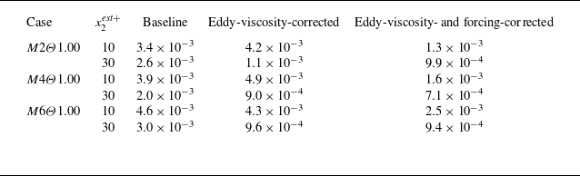
 Eu1
 x2meas+=50

 x2meas+=50
 x2est+=10
 M2Θ1.00
 a
 b
 c
 d

 x2meas+=50
 x2est+=30
 M2Θ1.00
 a
 b
 c
 d

 x2meas+=50
 a
 x2est+=10
 b
 x2est+=30
 M2Θ1.00

 x2meas+=50
 x2est+=10
 M4Θ1.00
 a
 b
 c
 d

 x2meas+=50
 x2est+=30
 M4Θ1.00
 a
 b
 c
 d

 x2meas+=50
 a
 x2est+=10
 b
 x2est+=30
 M4Θ1.00

 x2meas+=50
 x2est+=10
 M6Θ1.00
 a
 b
 c
 d
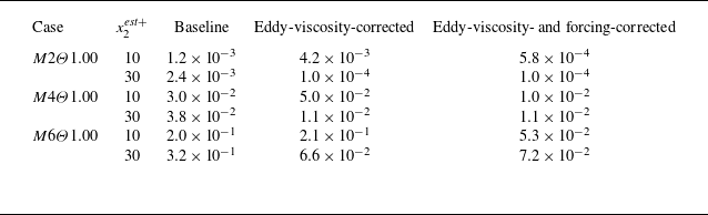
 ET
 x2meas+=50

 x2meas+=50
 x2est+=30
 M6Θ1.00
 a
 b
 c
 d

 x2meas+=50
 a
 x2est+=10
 b
 x2est+=30
 M6Θ1.00

 a,c,e
 b,d,f
 x2meas+=50
 a,b
 M2Θ1.00
 c,d
 M4Θ1.00
 e,f
 M6Θ1.00

 a,c
 b,d
 x2meas+=50
 a,b
 M2Θ0.25
 c,d
 M6Θ0.25

 a
 b

 x2meas+=50
 x2est+=10
 M2Θ0.25
 a
 b
 c
 d

 x2meas+=50
 x2est+=30
 M2Θ0.25
 a
 b
 c
 d

 x2meas+=50
 a
 x2est+=10
 b
 x2est+=30
 M2Θ0.25

 x2meas+=50
 x2est+=10
 M6Θ0.25
 a
 b
 c
 d

 x2meas+=50
 x2est+=30
 M6Θ0.25
 a
 b
 c
 d

 x2meas+=50
 a
 x2est+=10
 b
 x2est+=30
 M6Θ0.25

 x2meas+=50
 x2est+=10
 M2Θ0.25
 a
 b
 c
 d

 x2meas+=50
 x2est+=30
 M2Θ0.25
 a
 b
 c
 d

 x2meas+=50
 a
 x2est+=10
 b
 x2est+=30
 M2Θ0.25
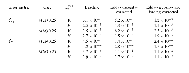
 x2meas+=50

 x2meas+=50
 x2est+=10
 M6Θ0.25
 a
 b
 c
 d

 x2meas+=50
 x2est+=30
 M6Θ0.25
 a
 b
 c
 d

 x2meas+=50
 a
 x2est+=10
 b
 x2est+=30
 M6Θ0.25



