1. Introduction

Selection can relate traits to environments in broadly two ways. On the one hand, a trait can evolve as an adaptation to the total undifferentiated environment. On the other hand, a trait can evolve as an adaptation to particular environmental conditions. The case of Endler’s (Reference Endler1983) guppies adapting to predation conditions seems to be such an example. The two are not mutually exclusive. Presumably, an adaptation to particular environmental conditions must also be an adaptation to the rest of the environment, if it is to fix by natural selection for it. Yet the converse need not be true. An adaptation to the entire environment need not be an adaptation to anything in particular; it might simply be advantageous to its bearers no matter the environment. Adaptations driven by pure r-selection (Lennox and Wilson Reference Lennox and Wilson1994) seem to be examples. I will call those traits that are also adaptations to particular environmental conditions adaptations to and will use adaptation simpliciter to denote traits that are at least adaptations to the total environment and possibly, in addition, adaptations to particular environmental conditions.

In this article, I offer an account of adaptation simpliciter that accommodates all cases of adaptation to particular environmental conditions sensu Glymour (Reference Glymour2011). Assuming adaptations to particular environmental conditions are a proper subset of adaptations simpliciter, I argue that the traditional account of adaptations handed down from Sober (Reference Sober1984; but see also Brandon Reference Brandon1990)—that it must be advantageous in some contexts and disadvantageous in none—is too stringent.Footnote ¹ I argue for a novel theory of adaptation in its place. I then consider the implications of this position.

Before beginning, some terminology needs to be emphasized. First, I assume the conception of causation from the causal modeling framework (Pearl Reference Pearl2000; Spirtes, Glymour, and Schienes Reference Spirtes, Glymour and Schienes2000; Woodward Reference Woodward2003). This will aid in understanding the relationship between the positions of Sober and Glymour. A trait variable Z and at least one environmental variable X (with values x codifying particular environmental features or conditions of kind X), for example, cause a reproductive success variable R if and only if there is some set of background conditions of which X = x (Z = z) is an element and in which changing Z (X) from Z = z′ (X = x′) to Z = z (X = x) would change the probability distribution over R. This can be expressed graphically as $Z\to R\leftarrow X$. The strength of these causal relationships can be, for our purposes, characterized in terms of the difference a hypothetical intervention on the exogenous causes makes to the expected reproductive success—or fitness—of organisms.

Second, in what follows it will be essential to distinguish between distinct environments. There are, in the literature, two ways of doing this. One can, as is commonly done, distinguish environments by the fitnesses of types in them (Brandon Reference Brandon1990; but see also Sober Reference Sober1984). This strategy conflates locations in which different causes operate to produce the same expectations for reproductive success. The presence or absence of interactions between such environmental causes of success and phenotypic causes of success will play a crucial role in the arguments to come. Hence, I instead adopt the alternative strategy (Glymour Reference Glymour2011) and individuate environments in terms of the values taken by variables measuring environmental causes of reproductive success.Footnote ²

2. Sober on Adaptations

For Neo-Darwinists, selection and luck—drift in its sundry forms—are distinct sources of evolution. Adaptations are to be explained by appeals to selection rather than drift. Sober seeks to define ‘adaptation’ so as to preserve the intuition that adaptations are driven to fixation by selection alone. So, he rules out averaging across certain environments that types happen to find themselves in by insisting that adaptations be positive causal factors for reproductive success. That is, adaptations must have increased expected reproductive success for some bearers and decreased it for none in the environments actually occupied by the species in which the adaptations arose. He defines an adaptation as follows: trait z is an adaptation in population p if and only if z became prevalent in p because there was evolution by natural selection for z (cf. Sober Reference Sober1984, 208).

Sober holds that there is selection for Z = z if and only if individuals vary with respect to whether they have Z = z and having Z = z is a positive causal factor for the reproductive successes of individuals in the population (Reference Sober1984, 280). Finally, according to Sober, a trait is a positive causal factor for an outcome if and only if the trait increases the probability of the outcome for some individuals and decreases it for none (294).

Sober employs a conception of causation on which properties are the causal relata rather than variables. Interpreting Sober’s view on adaptation in the causal modeling framework used here, we have what follows. Let X be a set of environmental variables (a set of kinds of features or conditions) each of which causes reproductive success R but none of which has a causal connection to trait variable Z. These comprise the “causally relevant background conditions” (Sober Reference Sober1984, 289–91). Then, Sober’s view requires that fixed trait Z = z is an adaptation only if, for all $X\in X$, Z causes R such that

• (S1) for some environmental condition X = x the fitness of organisms with Z = z in X = x is higher than that of organisms with any alternative Z = z′ and

• (S2) for no environmental condition X = x is there some alternative Z = z′ such that the fitness of organisms with Z = z in X = x is less than that of organisms with Z = z′.

Constraints S1 and S2 imply that the adaptation was a positive causal factor for reproductive success. Z = z is not an adaptation if, for some $X\in X$, the expected reproductive success of organisms with Z = z was ever lower than that of organisms with any alternative Z = z′ across the values of X. In such an instance, Z = z fixed not as the result of selection but as the result of the chancy distribution of environments over types.Footnote ³

Sober’s account of adaptation has been widely accepted, in part because it is explicitly causal and in part because of the way in which it uses the requirement that traits be positive causal facts to avoid counterintuitive results that would otherwise follow from so-called illicit averaging. In other words, it makes sense of ‘common environments’ in which fitnesses comparisons are to be conducted (see also Brandon’s [Reference Brandon1990] formulation of adaptation). Virtually everyone agrees that selection requires a common environment in which to act, and the conditions encoded in S1 and S2 make good on this idea.Footnote ⁴ Consider an example. Suppose we have a population of spotted guppies with two different spot color types, one muted type with five bright spots (S = 5) and another gaudy type that has 15 bright spots (S = 15). Assume S has heritability 1. Suppose the number of offspring F is caused by the number of spots S an individual has, the number of predators P (0, 1, or 2) in the individual’s surroundings, and the temperature T (with values 10°C and 20°C) in the individual’s surroundings, according to the equation

$\text{E}\left(F|S,P,T\right)=20+S-SP+T\mathrm{.}$

Importantly, assume there is no causal connection between any of the causes of number of offspring so that they are all exogenous, and note that, whereas S makes a contribution to F that depends on the value of P, there is not any context dependency between S and T or between P and T. Finally, suppose that parents are replaced by offspring at random from the offspring pool, with a probability that is independent of type, so that the population size is constant.

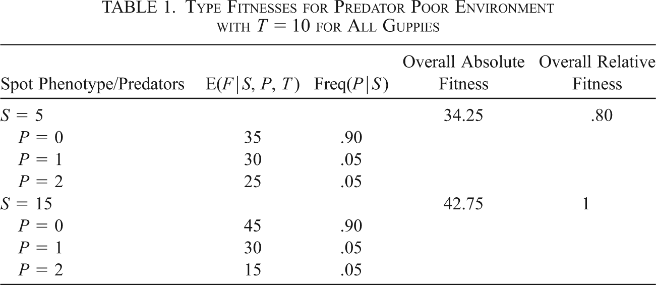
Suppose that the initial population was an even mix of the two types. Assume that T = 10 for all guppies and that mostly no predators (P = 0) characterize the initial environment. Suppose that in P = 0 environments the gaudy individuals stand out from their muted peers and attract more mates, such that changing from S = 5 to S = 15 would increase fitness. By contrast, under the condition of P = 2 the muted individuals blend in to their background better than their gaudy cousins and have a greater chance of surviving to reproductive age, such that changing from S = 15 to S = 5 would increase fitness. Because P is biased toward 0 under the initial conditions, the gaudy S = 15 type probably outcompetes the muted S = 5 type. This can be seen from the “overall absolute fitness” column calculated as the arithmetic mean given specific frequencies 0.90, 0.05, and 0.05 for P = 0, P = 1, and P = 2, respectively, as in table 1.Footnote ⁵

Table 1.

Type Fitnesses for Predator Poor Environment with T = 10 for All Guppies

Spot Phenotype/Predators	E(F|S, P, T)	Freq(P|S)	Overall Absolute Fitness	Overall Relative Fitness
S = 5			34.25	.80
P = 0	35	.90
P = 1	30	.05
P = 2	25	.05
S = 15			42.75	1
P = 0	45	.90
P = 1	30	.05
P = 2	15	.05

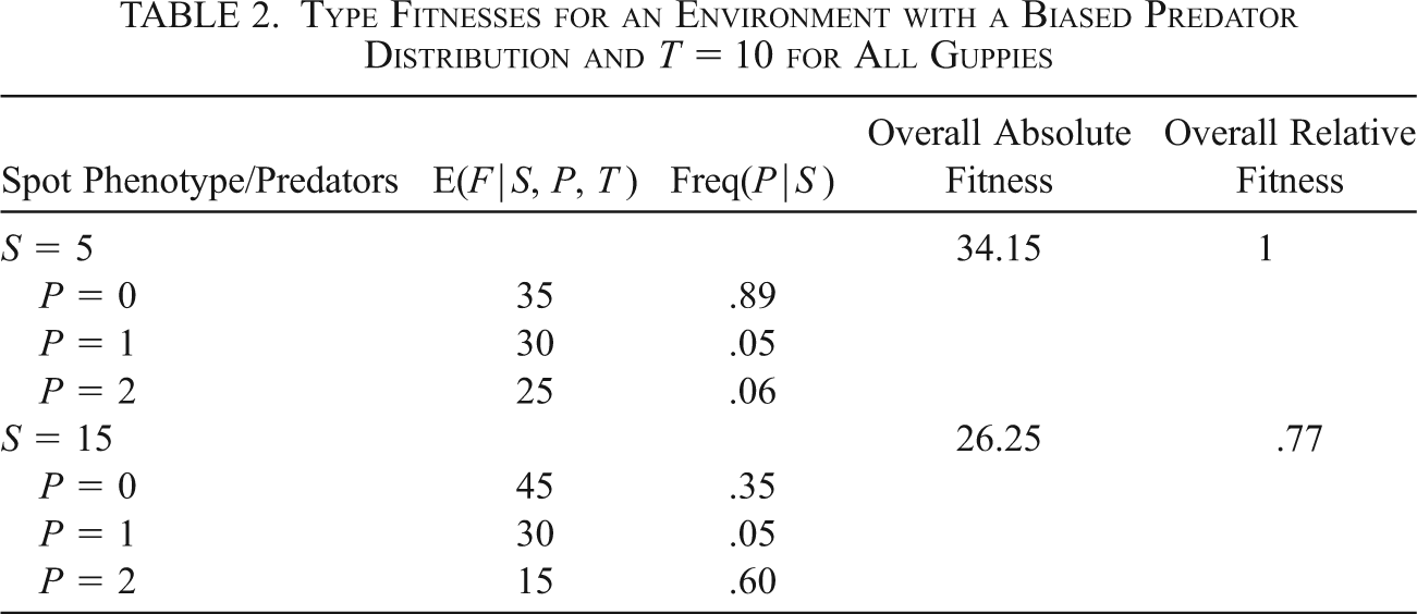
Type S = 15 has the higher fitness, and so, absent drift, it is expected to evolve. Suppose, however, that the distribution of the environmental variable P changes after some number of generations (say five). Subsequent to the change P is distributed over S such that S = 5’s are disproportionately in P = 0 and S = 15’s are disproportionately in P = 2. If the bias is sufficiently large, then when overall reproductive successes are calculated by averaging over the realized environmental conditions the muted five-spot type clearly has the advantage and will evolve if the environment does not revert. This can be gleaned from table 2.Footnote ⁶ Assume that the five-spot type does in fact fix in the novel environment. Given that a trait evolved that had the higher fitness, we might regard the fixed type as an adaptation (cf. Millstein Reference Millstein2002). However, this cannot be quite right.

Table 2.

Type Fitnesses for an Environment with a Biased Predator Distribution and T = 10 for All Guppies

Spot Phenotype/Predators	E(F|S, P, T)	Freq(P|S)	Overall Absolute Fitness	Overall Relative Fitness
S = 5			34.15	1
P = 0	35	.89
P = 1	30	.05
P = 2	25	.06
S = 15			26.25	.77
P = 0	45	.35
P = 1	30	.05
P = 2	15	.60

The envisaged fixation of the S = 5 type depends on two things: the trait variable’s causal influence on the number of offspring under each level of predation and the chancy or accidental distribution of environments, qua number of predators, over types. Intuitively, the frequency of the five-spot type did not increase because there was unequivocal selection for muted types. Rather, there was evolution toward the muted types because of the chance draw of environments for the types. The five-spot type merely got lucky for many generations.

Sober’s theory delivers the intuitively correct result exactly because he requires adaptations to have been positive causal factors for reproductive success. In the case of our toy example, S2 is not met with respect to the environments the evolving population occupied in the latter part of the lineage before fixation. There were some members of the evolving population that experienced conditions under which having trait S = 5 was disadvantageous. So, it is not the case that S = 5 is an adaptation on fixation. It evolves merely because of the chancy distribution of types into environments in favor of the muted type.

3. Glymour on Adaptations to Particular Environmental Conditions

Sober’s theory is naturally read as an account of adaptation simpliciter. Certainly when a trait was a positive causal factor for reproductive success, the trait is an adaptation no matter the environment. But Glymour’s view is one that (at least sometimes) diagnoses traits as adaptations to specific environmental features. Biologists are sometimes intent on showing how traits are adaptations to particular environmental variables. For example, as I mentioned before, Endler’s (Reference Endler1983) research on guppies is paradigmatic in this respect. Other famed cases include Darwin’s finches (Price et al. Reference Price, Grant, Gibbs and Boag1984; Gibbs and Grant Reference Gibbs and Grant1987) and Kettlewell’s (Reference Kettlewell1973) moths. Recent studies on high-crowned teeth in ungulates in grassland environments are revealing as well (Heywood Reference Heywood2010). These studies make no sense unless they are responsive to concern for adaptations to. The two conceptions of adaptations are not strictly incompatible. Yet adaptations to are importantly different from adaptations simpliciter, and sometimes Sober’s and Glymour’s theories deliver conflicting diagnoses of traits.

To see this, let us start with what Glymour takes to be necessary for the concept ‘adaptation to’. For Glymour if we are to identify one rather than another set of features of the environment as features to which a species is adapting, those features must explain why the differences in fitness among phenotypes is one way rather than another, even when those features are homogeneously distributed over types in the population. This is only possible if the environmental features are an interactive cause of reproductive success (cf. Glymour Reference Glymour2011, 464). Glymour holds that features of kind X are homogeneously distributed over traits Z if and only if, for all values of X and all pairs of values Z = z and Z = z′, $\text{Freq}(X=x|Z=z)=\text{Freq}(X=x|Z=z^{\prime })$ (Reference Glymour2011, 465). Moreover, although Glymour does not explicitly define it this way, he means by ‘interactive causation’ a special kind of interaction or context dependency. If Z = z is the supposed adaptation arising from interactive causation, then the difference in fitness made by changing from Z = z′ to Z = z in some X = x contexts is positive, whereas the difference in fitness made by changing from Z = z′ to Z = z in some alternative X = x′ contexts is not positive.

Glymour’s view can be rendered in analogous fashion to Sober’s. Let X be a set of environmental variables each of which causes reproductive success R but none of which has a causal connection to trait variable Z. Then, Glymour’s view requires that fixed trait Z = z is an adaptation to environmental features of kind $X\in X$ only if Z and X interact to cause R such that

• (G1) for some environmental condition X = x the fitness of organisms with Z = z in X = x is higher than that of organisms with any alternative Z = z′ and

• (G2) for some other environmental condition X = x′ there is some alternative Z = z′ such that the fitness of organisms with Z = z in X = x′ is not greater than that of organisms with Z = z′.

Constraints G1 and G2 imply that the relevant environmental conditions interacted with a trait variable in just the right way to cause reproductive success. Return to our guppy example once more to see how this works.

Suppose that P and T are homogeneously distributed over S as in the initial environment (table 1). Homogeneity-preserving interventions on T can change the rate at which the population evolves but cannot change the fact that S = 15 probably fixes in the population. Increasing T from 10°C to 20°C merely increases everyone’s fitness by 10 offspring but does not change the ordinal relation among the fitnesses. Thus, no actual distribution of T can be used to explain the evolution of S = 15 as an adaptation. If the actual distribution of temperature is homogeneous and contrasting alternatives are too, then the same S value is expected to evolve in either case. If the actual distribution is not homogeneous, then the evolution of S is a matter of drift—the chancy assignment of one rather than another type to favorable environments—rather than a matter of the superiority of one type over the other in a common environment (cf. Glymour Reference Glymour2011, 466).

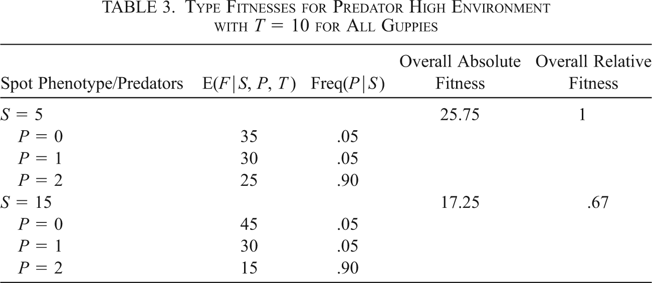
Yet, according to Glymour, P is different. Changes in the distribution of P can change the direction of selection even when the new distribution is homogeneous; that is, both the initial and new distribution of types to environments are such that the frequency with which five-spot guppies find themselves in low-predator environments remains equal to the frequency with which 15-spot guppies find themselves in low-predation environments. So suppose that when P changed it turned out that many members (0.90) of the lineage experienced two predators while a few members (0.10) experienced one or zero predators, yet P continued to be homogeneously distributed over S. Given this and the assumption that the environment does not change again, when overall reproductive successes are calculated by averaging over the realized environmental conditions, the muted five-spot type clearly has the advantage. Assuming T = 10 for all guppies, this can be gleaned from table 3.Footnote ⁷ In contrast to the situation described in table 1, type S = 5 now has the higher fitness, and it is expected to evolve in the homogeneous environment; this change has nothing to do with T, which increases the number of offspring of all guppies by 10, and everything to do with the new, yet homogeneous, distribution of P.

Table 3.

Type Fitnesses for Predator High Environment with T = 10 for All Guppies

Spot Phenotype/Predators	E(F|S, P, T)	Freq(P|S)	Overall Absolute Fitness	Overall Relative Fitness
S = 5			25.75	1
P = 0	35	.05
P = 1	30	.05
P = 2	25	.90
S = 15			17.25	.67
P = 0	45	.05
P = 1	30	.05
P = 2	15	.90

Precisely because P interacts with S in a special way, a change from one to another homogeneous distribution of it can influence the direction of selection, and hence the evolution of S = 5 rather than S = 15 is explained in part by the homogeneously distributed P (cf. Glymour Reference Glymour2011, 466). This is because, had it been different—as in the actually realized initial environment—the ordinal relation among type fitnesses would have been different. Hence, on Glymour’s view the muted S = 5 type is an adaptation to the number of predators in our new case (table 3).

Note, however, that on Sober’s account the S = 5 type is not an adaptation at all, because in the current case, as in the original case, condition S2 is violated. There were some members of the evolving population that experienced conditions under which having trait S = 5 was disadvantageous. This can be seen again in table 3. Hence, the fixed trait was not a positive causal factor for reproductive success in the environments actually occupied by the species in which the adaptation arose. Therefore, Glymour’s theory and the positive causal factor theory of Sober conflict (at least) in this case.

To be clear, the theories do not conflict in other similar cases. If G2 is satisfied because, but only because, there are some members that occupy environments X = x′ in which organisms with Z = z and organisms with some alternative Z = z′ are equally fit, while all others occupy environments X = x in which organisms with Z = z are fitter than organisms with any alternative Z = z′, Sober’s account will yield the result that Z = z is an adaptation on fixation, and Glymour’s account will yield the compatible result that it is also an adaptation to environmental conditions of kind X. But, as I have argued, whenever there is any member of the population inhabiting an environment (say, X = x′) in which Z = z′ is actually fitter than Z = z, Glymour’s account can correctly render Z = z an adaptation to environmental conditions of kind X, while Sober’s account will always, incompatibly, yield the conclusion that Z = z is not an adaptation at all.

4. A Theory of Adaptation

The predation variable in the case of the guppies interacts with the spot variable to cause reproductive success by controlling the way in which the spot variables influence reproductive success. Under some conditions gaudy guppies are selected for, whereas under other conditions muted guppies are selected for. Endler (Reference Endler1983) managed to experimentally induce a change in the direction of evolution by changing environmental variables. Nature, however, is often not as exacting as experimental setups. It is easy to conceive of the muted type with less bright spots going to fixation in an environment characterized by a range of predation, even though it was inferior earlier in the lineage in an environment characterized by no predation. In such circumstances, Glymour’s view and the view of Sober imply inconsistent diagnoses of the trait on its fixation in the population. Glymour’s view implies that the fixed trait is an adaptation to the predation variable. Sober’s view implies that the fixed trait is not an adaptation and so a fortiori not an adaptation to the predation variable. This is because he is committed to the view that adaptations were positive causal factors for reproductive success.

The correct response to this conflict, I propose, is to accept both adaptations simpliciter and adaptations to. However, we can be pluralists only if we give up on the idea that adaptations necessarily were positive causal factors for reproductive success and, in particular, give up on constraint S2. Although there seem to be adaptations that are not adaptations to anything in particular, it is a reasonable assumption that all adaptations to must also be adaptations simpliciter. Given this assumption, Sober cannot be right to require that adaptations were positive causal factors for reproductive success. For, if we follow him in requiring this, we end up denying that certain adaptations to are adaptations simpliciter, as, for example, in our toy case with strictly homogeneous environments. So, contrary to Sober, in that case, the muted type—which is an adaptation to the number of predators P—must also be an adaptation simpliciter.Footnote ⁸

As far as adaptations to particular environmental conditions go, then, let us stick with Glymour’s constraints codified in G1 and G2. For adaptations simpliciter let us drop S2. Let X be a set of environmental variables each of which causes reproductive success R but that have no causal connection to trait variable Z. Then fixed trait Z = z is an adaptation to the whole environment X only if, for all $X\in X$, Z causes R such that for some environmental condition X = x the fitness of organisms with Z = z in X = x is higher than that of organisms with any alternative Z = z′. This simply means that there was some environmental condition X = x such that changing Z from Z = z′ to Z = z would increase fitness. On the theory of adaptations simpliciter here, all adaptations to are also adaptations simpliciter as desired.

5. Implications

Given the centrality in biology of the idea that adaptations are sometimes adaptations to particular environmental conditions, I think we have little choice but to reject the requirement that adaptations exert a uniform positive influence on reproductive success. If we insist on it, we will not only have to give up on the idea that coloration is an adaptive response to predation, that hypsodonty is an adaptive response to some feature of grasslands, and that bill depth is an adaptive response to seed frequency. We will also have to give up on the idea that changes in environmental conditions drive evolutionary responses by means of selection within a lineage. If the frequency of distinct environments changes and that change drives the evolution of a once rare and disfavored type, this is because the environment variable and the trait variable interactively cause reproductive success. It will then follow that the evolved trait had a negative influence on reproductive success overall before the change and a positive influence overall after the change. Such traits do not have a uniformly positive influence on reproductive success and a fortiori cannot be adaptations unless we relinquish the requirement.

Doing so has both theoretical and practice implications. Here I examine just two. Individuating environments by vectors of values for environmental causes of reproductive success is essential for any account of adaptation to. It is essential for various other tasks too—for example, accounting for phenotypic plasticity and local coadaptation—as Glymour (Reference Glymour2011) has argued. More important for us, this move offers machinery for explaining where and why the evolution of a population is dominated by drift and where and why the population is dominated by selection. We have evolution by drift when we have a heterogeneous distribution of environmental causes, but on any homogeneous distribution of the environmental variables the ordinal relations between fitnesses would be reversed. It is just such cases that Sober’s requirement that causes exert a uniformly positive influence is meant to exclude. Unfortunately, the requirement goes to far, excluding also cases in which relevant environmental conditions are homogeneously distributed over types but interact with the type variables to cause reproductive success (the paradigm case of adaptation to for Glymour). Still, given that environmental conditions are essentially never strictly homogeneously distributed over types, further elaborations of the theories articulated herein will be required. But the proper elaborations must tread carefully: as one weakens the assumption of homogeneous distributions, one invites illicit averaging—that is, treating cases of drift-driven evolution, in the form of the disproportionate representation of a less fit type in a more favorable environment, as cases of selection-driven adaptation. A full discussion would take us well beyond the scope of this article, but it is sufficient here to note that any account of adaptation will need to confront this issue in one way or another, and the current account has the virtue of pressing the point directly.

The framework for understanding the relation between adaptation and drift suggested above has a substantive implication concerning biological practice as well. Given the framework, it is only by modeling the causal influence of environmental variables explicitly that one can distinguish between traits driven to fixation by selection rather than by drift. The point is related to a point already made by Glymour (Reference Glymour2011). Glymour notes that evolutionary biologists sometimes do not explicitly model environmental conditions. Instead they condition on the environment as a whole. For example, population genetics models employ a fitness parameter for each type. The parameter can be seen as an estimate of the disposition for the type to survive and reproduce in the environment as a whole. Hence, these parameters can also be seen as an estimate of overall habitat quality from the type’s point of view. Sometimes such models can be used to diagnose when drift goes against what one would expect from selection (e.g., Brandon Reference Brandon1990). However, such models cannot do so reliably on the view of the relationship between adaptation and drift given in the last paragraph.

Suppose we collect data on an individual trait variable and individual reproductive success for various spatiotemporal locations without measuring any environmental conditions in those locations. For each location we estimate fitnesses and assess their ordinal relations across the locations. It might be that the ordinal relation among fitnesses is distinct across some locations. We can account for this in two ways, assuming none of the environmental conditions are causally connected with the focal trait variable. Either there are some homogeneously distributed environmental conditions that interact to cause reproductive success, or there are some heterogeneously distributed environmental conditions that cause reproductive success. In the latter case, the ordinal relation among fitnesses might differ between locations without interactive causation. To distinguish between the two cases, we would actually have to explicitly model the causal influence of the environmental variables rather than merely condition on various spatiotemporal locations. Hence, the verdict that a trait is an adaptation on fixation requires explicitly representing the causal influence of environmental variables.

6. Concluding Summary

Sober requires of adaptations that they were positive causal factors for reproductive success. Glymour’s work, however, entails that fixed traits are adaptations to specific environmental features only given a special sort of interactive causation. In some cases these positions provide inconsistent diagnoses. I argued that, given one such conflict, we ought to give up on the idea that adaptations must have been positive causal factors for reproductive success. On grounds that all adaptations to specific environmental features are adaptations simpliciter, Sober cannot be right to require this of adaptations. I provide a rectification of the two theories and use it to highlight two implications for evolutionary biology. Theoretically, the concepts of adaptation and drift are inseparable, insofar as an account of adaptation will need to rely on a prior decision about which heterogeneous environments do and which do not constitute a form of drift. Also, in practice, various attempts to measure fitness, predict the consequences of fitness differences, and identify adaptations will turn out to require quantitative measures of the environmental causes of reproductive success.