2 A hemispherical radome

Consider steady rainfall on a radome surface covered by a periodic array of micro-scale pillars. Water from the rain flows down the slope in a thin layer which is bounded below by the pillar tops and air pockets and above by the atmosphere. We assume that the asperity is small enough so that the bottom surface is in a Cassie–Baxter state. Similar to the boundary layer over a superhydrophobic plate studied by Mei & Guo (Reference Mei and Guo2018), the radome problem is characterized by the existence of multiple length scales: the radome radius $R$ (macro-scale), the film thickness $h$ (meso-scale) and the pillar diameter and lattice spacing $\ell$ (micro-scale). The mathematical similarity is summarized in table 1.

Figure 1.

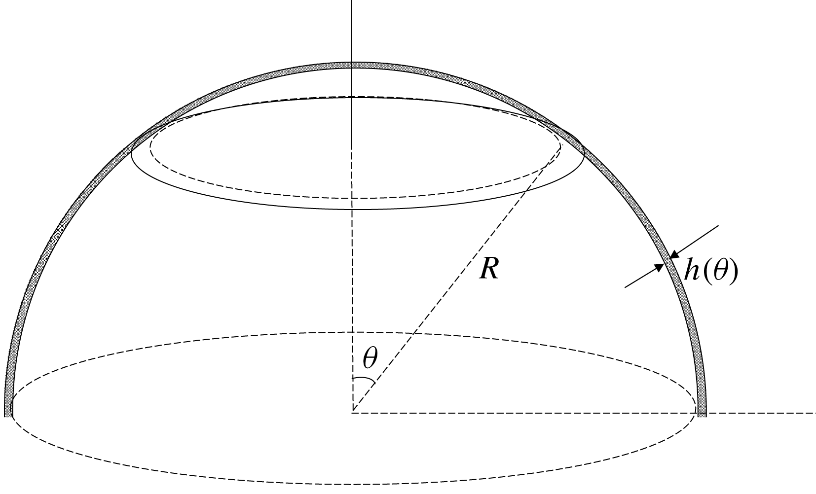
Spherical radome.

Table 1.

Resemblance of radome film and boundary layer on a flat plate.

2.1 Variations on the macro-scale

We denote the radial coordinate from the centre of the sphere by $r$ . Let $z=r-R\ll R$ be the coordinate normal to the film. The film depth $h$ is typically a fraction of 1 mm and vastly smaller than the radome radius $R(=O(10~\text{m}))$ which is the characteristic length in the flow direction; hence, convective acceleration is negligible. Assuming the flow to be laminar, the radial and azimuthal momentum equations in the region not too close to the textured bottom are respectively,

(2.1) $$\begin{eqnarray}\displaystyle & \unicode[STIX]{x1D70C}g\cos \unicode[STIX]{x1D703}=-{\displaystyle \frac{\unicode[STIX]{x2202}p}{\unicode[STIX]{x2202}z}},\quad 0<z<h; & \displaystyle\end{eqnarray}$$

(2.2) $$\begin{eqnarray}\displaystyle & 0=g\sin \unicode[STIX]{x1D703}+\unicode[STIX]{x1D708}{\displaystyle \frac{\unicode[STIX]{x2202}^{2}u}{\unicode[STIX]{x2202}z^{2}}},\quad 0<z<h, & \displaystyle\end{eqnarray}$$

where $p$ is the hydrodynamic pressure, $u$ the fluid velocity parallel to the surface and $\unicode[STIX]{x1D703}$ the azimuthal angle shown in figure 1. These approximations will be justified later. Because $h\ll R$ , the local free surface above the pillar is essentially parallel to the bottom. The free surface is assumed to be stress free, hence

(2.3) $$\begin{eqnarray}\frac{\unicode[STIX]{x2202}u}{\unicode[STIX]{x2202}z}=0,\quad z=h(\unicode[STIX]{x1D703}).\end{eqnarray}$$

Along the Cassie–Baxter bottom, slipping is allowed so that

(2.4) $$\begin{eqnarray}\frac{\unicode[STIX]{x2202}u}{\unicode[STIX]{x2202}z}=\frac{u}{\unicode[STIX]{x1D706}},\quad z=0,\end{eqnarray}$$

where $\unicode[STIX]{x1D706}$ is the local slip length.

The local velocity at any $\unicode[STIX]{x1D703}$ and $z$ is

(2.5) $$\begin{eqnarray}u(\unicode[STIX]{x1D703},z)=\frac{g}{\unicode[STIX]{x1D708}}\sin \unicode[STIX]{x1D703}\left(\unicode[STIX]{x1D706}h+hz-\frac{z^{2}}{2}\right),\quad 0<z<h.\end{eqnarray}$$

The total outflux across a circular ring at $\unicode[STIX]{x1D703}$ is

(2.6) $$\begin{eqnarray}2\unicode[STIX]{x03C0}R\sin \unicode[STIX]{x1D703}\int _{0}^{h}\,\text{d}z\,u(z,\unicode[STIX]{x1D703})=2\unicode[STIX]{x03C0}R\sin ^{2}\unicode[STIX]{x1D703}\frac{g}{\unicode[STIX]{x1D708}}\left(\unicode[STIX]{x1D706}h^{2}+\frac{h^{3}}{3}\right).\end{eqnarray}$$

On the other hand, the influx from the rain falling into the horizontal circle above the same ring is $Q\unicode[STIX]{x03C0}R^{2}\sin ^{2}\unicode[STIX]{x1D703}$ where $Q$ is the rate of rainfall. Equating the two fluxes we find

(2.7) $$\begin{eqnarray}Q\unicode[STIX]{x03C0}R^{2}\sin ^{2}\unicode[STIX]{x1D703}=2\unicode[STIX]{x03C0}R\sin ^{2}\unicode[STIX]{x1D703}\frac{g}{\unicode[STIX]{x1D708}}\left(\unicode[STIX]{x1D706}h^{2}+\frac{h^{3}}{3}\right),\end{eqnarray}$$

i.e.

(2.8) $$\begin{eqnarray}QR=\frac{2g}{\unicode[STIX]{x1D708}}\left(\unicode[STIX]{x1D706}h^{2}+\frac{h^{3}}{3}\right).\end{eqnarray}$$

In terms of $H_{o}$ defined in (1.1), equation (2.8) becomes

(2.9) $$\begin{eqnarray}\frac{h^{3}}{H_{o}^{3}}+3\frac{\unicode[STIX]{x1D706}}{H_{o}}\frac{h^{2}}{H_{o}^{2}}-1=0\end{eqnarray}$$

which can be exactly solved.

In the hydrophilic limit, $\unicode[STIX]{x1D706}=0$ , $h=H_{o}$ as derived by Gibble. From here on, we shall define the velocity over the smooth radome as the base flow

(2.10) $$\begin{eqnarray}u_{B}(z,\unicode[STIX]{x1D703})=\frac{g}{\unicode[STIX]{x1D708}}\sin \unicode[STIX]{x1D703}\left(H_{o}z-\frac{z^{2}}{2}\right)\end{eqnarray}$$

whose maximum velocity occurs on the free surface at the equator

(2.11) $$\begin{eqnarray}U_{o}\equiv \frac{gH_{o}^{2}}{2\unicode[STIX]{x1D708}}.\end{eqnarray}$$

To confirm the basic assumptions, let us consider the hydrophilic limit and take $R=20~\text{m}$ , $Q=50~\text{mm}~\text{h}^{-1}$ , $\unicode[STIX]{x1D70C}=1~\text{g}~\text{cm}^{-3}$ , $g=980~\text{cm}~\text{s}^{-2}$ , $\unicode[STIX]{x1D707}=10^{-2}~\text{g}~\text{cm}^{-1}~\text{s}^{-1}$ , then the maximum film thickness is $H_{o}=0.342~\text{mm}$ . The maximum velocity at the equator is $U_{o}=57.31~\text{cm}~\text{s}^{-1}$ . The ratio of convective inertia to viscous force can be estimated by $O((u/R)(\unicode[STIX]{x2202}u/\unicode[STIX]{x2202}\unicode[STIX]{x1D703})/\unicode[STIX]{x1D708}(\unicode[STIX]{x2202}^{2}u/\unicode[STIX]{x2202}z^{2}))=1.6422/636.8=0.00258\ll 1$ which is small enough to justify (2.1) and (2.2). Note that the maximum Reynolds number in the mean flow is finite $Re_{h}=U_{o}H_{o}/\unicode[STIX]{x1D708}=196$ , implying laminarity.

2.2 Micro-scale cell problem and the slip length

As the texture in manufactured surface is likely uniform on the macro-scale, the radome is assumed to be covered by a square lattice of circular pillars of diameter $d$ spaced $\ell$ apart from centre to centre. This square lattice geometry can be quite accurately achieved on a spherical surface by positioning the pillars in the following way. Measuring the latitudinal angle $\unicode[STIX]{x1D703}$ from the north pole, we let there be $M$ circles defined by $\unicode[STIX]{x1D703}_{m}=m\unicode[STIX]{x1D6E5}$ with $\unicode[STIX]{x1D6E5}=\ell /R$ and $m=0,1,2,3,\ldots ,M$ so that $M\ell =(\unicode[STIX]{x03C0}/2)R$ . On each latitudinal circle of circumference $2\unicode[STIX]{x03C0}R\sin \unicode[STIX]{x1D703}_{m}$ , grid points equally separated by $\ell$ are marked. A square $\ell \times \ell$ array is therefore formed in the upper hemisphere. Because the total circumference of each circle may not be exactly an integral multiple of $\ell$ , minor imperfection of the lattice geometry may occur along a curve on the entire hemisphere. Any longitudinal arc should cross a line array of periodic cells with only slight off-centre deviations. Due to the vast contrast of length scales ( $O(\ell /R)=0.2~\text{mm}/20\,000~\text{mm}=10^{-5}\ll 1$ ), the background flow, which varies on the macro-scale, enters every micro-scale cell essentially normally, rendering this deviation inconsequential. Thus, with an error of $O(\ell /R)$ , the neighbourhood of every longitudinal circle can be considered as a square lattice on a flat plane.

Adopting the common model of a Cassie–Baxter state, we assume the base surface to be smooth and flat, with zero velocity on the flat pillar tops, and zero shear stress on the interface above the air pockets. Within each cell of dimensions $\ell \times \ell \times h$ , the fluid velocity  $\boldsymbol{u}$ is the sum of  $u_{B}\boldsymbol{e}_{x}$ and perturbation $\tilde{\boldsymbol{u}}\,=\,(\tilde{u} ,\tilde{v},\tilde{w})$ , i.e. $\boldsymbol{u}\,=\,u_{B}\boldsymbol{e}_{\boldsymbol{x}}\,+\,\tilde{\boldsymbol{u}}$ . Since in the $O(\ell )$ neighbourhood above the base, i.e. the near field, the perturbed velocities $(\tilde{u} ,\tilde{v},\tilde{w})$ must be of $O((\ell /H_{o})U_{o})$ , we introduce the following normalization

(2.12a-c ) $$\begin{eqnarray}\boldsymbol{x}=\ell \boldsymbol{x}^{\prime },\quad \tilde{\boldsymbol{u}}=U_{o}\frac{\ell }{H_{o}}\tilde{\boldsymbol{u}}^{\prime },\quad \tilde{p}=\unicode[STIX]{x1D707}\frac{U_{o}}{\ell }\frac{\ell }{H_{o}}\tilde{p}^{\prime },\end{eqnarray}$$

where $U_{o}$ is defined by (2.11) and all normalized variables are distinguished by primes. We shall also normalize the film depth by $\ell$ ,

(2.13) $$\begin{eqnarray}h=\ell h^{\prime }\end{eqnarray}$$

with the allowance that $h^{\prime }\geqslant O(1)$ .

For $\tilde{\boldsymbol{u}}$ , the Cartesian coordinates $\boldsymbol{x}=(x,y,z)$ are local and centred around the pillar. Dependence on $\unicode[STIX]{x1D703}$ will not be shown for brevity. Rewritten in normalized variables, the basic flow velocity is

(2.14) $$\begin{eqnarray}\displaystyle & u_{B}^{\prime }(\unicode[STIX]{x1D703},z^{\prime })=2\sin \unicode[STIX]{x1D703}\left(z^{\prime }{\displaystyle \frac{\ell }{H_{o}}}-{z^{\prime }}^{2}{\displaystyle \frac{\ell ^{2}}{2{H_{o}}^{2}}}\right), & \displaystyle\end{eqnarray}$$

(2.15) $$\begin{eqnarray}\displaystyle & \boldsymbol{u}^{\prime }=\left[u_{B}^{\prime }(\unicode[STIX]{x1D703},z^{\prime })\boldsymbol{e}_{\boldsymbol{x}}+{\displaystyle \frac{\ell }{H_{o}}}\tilde{\boldsymbol{u}}^{\prime }(\boldsymbol{x}^{\prime })\right]. & \displaystyle\end{eqnarray}$$

Because of the finite Reynolds number in the basic flow, the perturbed flow in the microcells must be governed by the full Navier–Stokes equations, which are

(2.16) $$\begin{eqnarray}\displaystyle & \unicode[STIX]{x1D735}\boldsymbol{\cdot }\tilde{\boldsymbol{u}}^{\prime }=0, & \displaystyle\end{eqnarray}$$

(2.17) $$\begin{eqnarray}\displaystyle & Re_{\ell }\left[{\displaystyle \frac{H_{o}}{\ell }}u_{B}^{\prime }{\displaystyle \frac{\unicode[STIX]{x2202}\tilde{\boldsymbol{u}}^{\prime }}{\unicode[STIX]{x2202}x^{\prime }}}+\tilde{\boldsymbol{u}}^{\prime }\boldsymbol{\cdot }\unicode[STIX]{x1D735}\tilde{\boldsymbol{u}}^{\prime }+\tilde{w}^{\prime }{\displaystyle \frac{H_{o}}{\ell }}{\displaystyle \frac{\unicode[STIX]{x2202}u_{B}^{\prime }}{\unicode[STIX]{x2202}z^{\prime }}}\boldsymbol{e}_{\boldsymbol{x}}\right]=-\unicode[STIX]{x1D735}\tilde{p}^{\prime }+\unicode[STIX]{x1D6FB}^{2}\tilde{\boldsymbol{u}}^{\prime }, & \displaystyle\end{eqnarray}$$

where

(2.18) $$\begin{eqnarray}Re_{\ell }=\frac{U_{o}\ell }{\unicode[STIX]{x1D708}}\frac{\ell }{H_{o}}\end{eqnarray}$$

is the Reynolds number for the cell problem.

The bottom surface $S$ is composed of the flat pillar tops $S_{s}$ and the water surface $S_{f}$ above the air pockets. On $S_{s}$ , there is no slip,

(2.19a,b ) $$\begin{eqnarray}u_{B}^{\prime }(0)=0,\quad \text{and}\quad \tilde{\boldsymbol{u}}^{\prime }=0,\quad z^{\prime }=0,\boldsymbol{x}^{\prime }\in S_{s}.\end{eqnarray}$$

Ignoring the presence of air, there is no shear stress on $S_{f}$ ,

(2.20) $$\begin{eqnarray}\frac{\unicode[STIX]{x2202}u}{\unicode[STIX]{x2202}z}=\frac{U_{o}}{\ell }\left[\frac{\unicode[STIX]{x2202}u_{B}^{\prime }}{\unicode[STIX]{x2202}z^{\prime }}+\frac{\ell }{H_{o}}\frac{\unicode[STIX]{x2202}\tilde{u} ^{\prime }}{\unicode[STIX]{x2202}z^{\prime }}\right]_{0}=0,\quad z^{\prime }=0,\boldsymbol{x}^{\prime }\in S_{f}\end{eqnarray}$$

i.e.

(2.21) $$\begin{eqnarray}\frac{\unicode[STIX]{x2202}\tilde{u} ^{\prime }}{\unicode[STIX]{x2202}z^{\prime }}=\left.-\frac{H_{o}}{\ell }\frac{\unicode[STIX]{x2202}u_{B}^{\prime }}{\unicode[STIX]{x2202}z^{\prime }}\right|_{0}=-2\sin \unicode[STIX]{x1D703},\quad z^{\prime }=0,\boldsymbol{x}^{\prime }\in S_{f}\end{eqnarray}$$

and

(2.22) $$\begin{eqnarray}\frac{\unicode[STIX]{x2202}\tilde{v}^{\prime }}{\unicode[STIX]{x2202}z^{\prime }}=0,\quad \tilde{w}^{\prime }=0,\quad z^{\prime }=0,\boldsymbol{x}_{\boldsymbol{ i}}^{\prime }\in S_{f}.\end{eqnarray}$$

On the free surface $z^{\prime }=h^{\prime }=h/\ell$ , we require

(2.23) $$\begin{eqnarray}\frac{\unicode[STIX]{x2202}\tilde{u} ^{\prime }}{\unicode[STIX]{x2202}z^{\prime }}=\left.-\frac{H_{o}}{\ell }\frac{\unicode[STIX]{x2202}u_{B}^{\prime }}{\unicode[STIX]{x2202}z^{\prime }}\right|_{h^{\prime }}=-2\sin \unicode[STIX]{x1D703}\left(1-h^{\prime }\frac{\ell }{H_{o}}\right)\neq 0,\end{eqnarray}$$

and

(2.24a,b ) $$\begin{eqnarray}\frac{\unicode[STIX]{x2202}\tilde{v}^{\prime }}{\unicode[STIX]{x2202}z^{\prime }}=0,\quad \tilde{w}^{\prime }=0.\end{eqnarray}$$

In addition, we require that $\tilde{\boldsymbol{u}}^{\prime },\tilde{p}^{\prime }$ are periodic on opposite boundaries of the square cell.

The micro- and macro-scale problems are coupled, and must be solved iteratively. One takes $h^{\prime }(\unicode[STIX]{x1D703})=H_{o}/\ell =\text{const.}$ as the first guess and solves $N$ micro-cell problems at discrete stations $\unicode[STIX]{x1D703}_{n}$ , $n=1,2,3,\ldots ,N$ along the circular arc $r=R,0<\unicode[STIX]{x1D703}_{n}<\unicode[STIX]{x03C0}/2$ . The inter-station spacing $R\unicode[STIX]{x0394}\unicode[STIX]{x1D703}$ will be chosen to be much larger than the cell size but much smaller than $R$ . After completing the solution in $N$ unit cells, area averages (denoted by angle brackets) are taken. The total mean velocity at level $z^{\prime }$ is then

(2.25) $$\begin{eqnarray}\displaystyle \left\langle \boldsymbol{u}(\boldsymbol{x})\right\rangle =U_{0}\langle \boldsymbol{u}^{\prime }(\boldsymbol{x}^{\prime })\rangle =U_{o}\left[u_{B}^{\prime }(\unicode[STIX]{x1D703})\boldsymbol{e}_{\boldsymbol{x}}+\frac{\ell }{H_{o}}\langle \tilde{\boldsymbol{u}}^{\prime }(\boldsymbol{x}^{\prime })\rangle \right], & & \displaystyle\end{eqnarray}$$

where angle brackets denote area averages over the cell base.

Since the total velocity vanishes over $S_{s}$ , the tangential velocity at the bottom is

(2.26) $$\begin{eqnarray}\left\langle u\right\rangle _{z=0}=U_{o}\left[(1-\unicode[STIX]{x1D719})\frac{\ell }{H_{o}}\left\langle \tilde{u} ^{\prime }\right\rangle _{f}\right]_{0},\end{eqnarray}$$

where $\unicode[STIX]{x1D719}$ is the solid fraction related to the area porosity $n$ by $n=1-\unicode[STIX]{x1D719}$ . The total shear stress vanishes over $S_{f}$ , hence,

(2.27) $$\begin{eqnarray}\left.\frac{\unicode[STIX]{x2202}\left\langle u\right\rangle }{\unicode[STIX]{x2202}z}\right|_{z=0}=\unicode[STIX]{x1D719}\frac{U_{o}}{\ell }\left[\frac{\text{d}u_{B}^{\prime }}{\text{d}z^{\prime }}+\frac{\ell }{H_{o}}\left\langle \frac{\unicode[STIX]{x2202}\tilde{u} ^{\prime }}{\unicode[STIX]{x2202}z^{\prime }}\right\rangle _{s}\right]_{0}.\end{eqnarray}$$

The normalized slip length $\unicode[STIX]{x1D706}^{\prime }$ follows from,

(2.28) $$\begin{eqnarray}\left\langle u^{\prime }\right\rangle =\unicode[STIX]{x1D706}^{\prime }\frac{\unicode[STIX]{x2202}\left\langle u^{\prime }\right\rangle }{\unicode[STIX]{x2202}z^{\prime }},\quad z^{\prime }=0;\end{eqnarray}$$

i.e.

(2.29) $$\begin{eqnarray}\unicode[STIX]{x1D706}^{\prime }(\unicode[STIX]{x1D703})\equiv \frac{\unicode[STIX]{x1D706}}{\ell }=\left[\frac{(1-\unicode[STIX]{x1D719}){\displaystyle \frac{\ell }{H_{o}}}\left\langle \tilde{u} ^{\prime }\right\rangle _{f}}{\unicode[STIX]{x1D719}\left({\displaystyle \frac{\text{d}u_{B}^{\prime }}{\text{d}z^{\prime }}}+{\displaystyle \frac{\ell }{H_{o}}}\left\langle {\displaystyle \frac{\unicode[STIX]{x2202}\tilde{u} ^{\prime }}{\unicode[STIX]{x2202}z^{\prime }}}\right\rangle _{s}\right)}\right]_{0}.\end{eqnarray}$$

This slip length is then used in (2.9) to find the updated $h$ at  $\unicode[STIX]{x1D703}$ .

3 Numerical procedure

The nonlinear boundary value problem on the micro-scale and the film thickness equation (2.9) are solved together by the following iterative procedure:

1. (i) A longitudinal arc $0<X=R\unicode[STIX]{x1D703}<L(=\unicode[STIX]{x03C0}R/2)$ is discretized into $N$ macro-stations ( $0<X_{1}<\cdots <X_{n}<\cdots <X_{N}=L$ ). At each station is a micro-scale cell with a square base extending from $z=0$ to $z=h_{i}$ where $h_{i}$ is the depth at the $i$ th iteration.

2. (ii) Gibble’s thickness (1.1) is chosen as the first iteration $h_{0}$ .

3. (iii) For a chosen solid fraction $\unicode[STIX]{x1D719}$ the perturbed flow in each cell is solved numerically by a finite element scheme.

4. (iv) The slip length $\unicode[STIX]{x1D706}_{1}(X_{n})$ of the first iteration is obtained from the cell solution at $N$ macro-stations.

5. (v) With the known $\unicode[STIX]{x1D706}_{1}(X_{n})$ , the first iteration of $h_{1}(X_{n})$ is obtained by solving (2.9).

6. (vi) The slip length $\unicode[STIX]{x1D706}_{2}(X_{n})$ at the next iteration is computed, which is used to obtain $h_{2}(X_{n})$ .

7. (vii) Repeat the iteration procedure from step $i$ to step $i+1$ until $|\unicode[STIX]{x1D706}_{i+1}-\unicode[STIX]{x1D706}_{i}|/\unicode[STIX]{x1D706}_{i}<10^{-4}$ .

In the finite element scheme, each unit cell is discretized into tetrahedral elements, each having 16 nodes. The unknowns $(\tilde{u} ,\tilde{v},\tilde{w},\tilde{p})$ are represented by linear interpolation functions. The unknown nodal coefficients are solved numerically. Approximately one million tetrahedral elements are distributed throughout the cell. Computations are performed in a Lenovo D30 workstation with dual Xeon5670 8-cores processors and 256 G memory. The typical computation time for the entire arc is four hours per set of input data. Typically six iterations are sufficient for convergence at the fourth digit. As a check, the total flux across a ring at any angle $\unicode[STIX]{x1D703}$ for different solid fractions $\unicode[STIX]{x1D719}$ is checked to be the same as that of the non-hydrophobic radome ( $\unicode[STIX]{x1D719}=0$ ). The procedure is similar to those in Mei & Guo (Reference Mei and Guo2018), where more details, including validations with works on flows of finite Reynolds numbers in micro-channels by Cheng et al. (Reference Cheng, Teo and Khoo2009), can be found.

We remark that at the radome top, $\unicode[STIX]{x1D703}=0$ , $u_{B}^{\prime }=\unicode[STIX]{x2202}u_{B}^{\prime }/\unicode[STIX]{x2202}z^{\prime }=0$ at $z^{\prime }=0$ . The perturbation velocity field $\left\langle \tilde{u} ^{\prime }\right\rangle _{f},\left\langle \unicode[STIX]{x2202}\tilde{u} ^{\prime }/\unicode[STIX]{x2202}z^{\prime }\right\rangle _{s}$ is trivially zero. Since the numerator and denominator of (2.29) both vanish, their ratio must be found from their limits near $\unicode[STIX]{x1D703}\approx 0$ . This will be detailed later.

4 Numerical results for a radome

Figure 2.

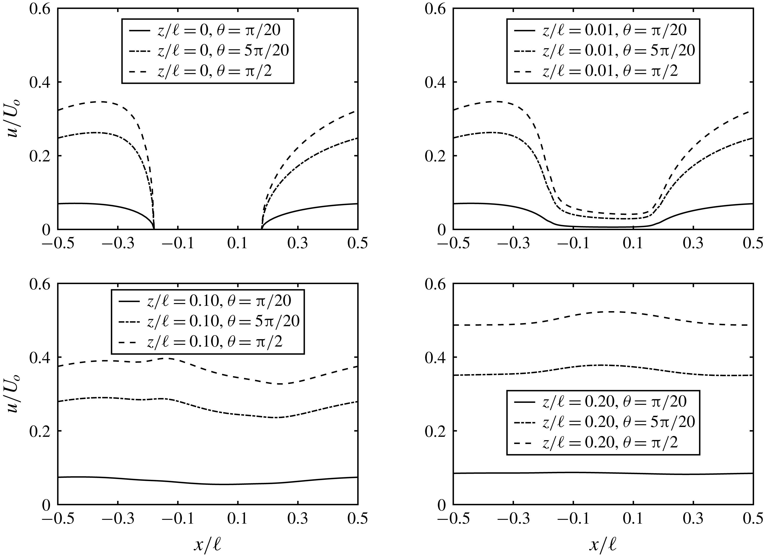
Variation of local horizontal velocity $\left\langle u(x,0,z)\right\rangle /U_{o}$ in a cell at different angular locations $\unicode[STIX]{x1D703}$ . Inputs are: $R=20~\text{m}$ , $\ell =0.18~\text{mm}$ , $d=0.0644~\text{mm}\;(\unicode[STIX]{x1D719}=0.10)$ , $Re_{\ell }=55.4$ .

Figure 2 shows the sample horizontal velocity at various heights in a unit cell, for cells at three different $\unicode[STIX]{x1D703}$ . Due to partial slipping at the bottom, departure from uniform flow is appreciable only in a narrow height of $O(\ell )$ near the bottom, as seen in figure 2(a,b). The total flow $\left\langle u^{\prime }\right\rangle$ is dominated by the basic parallel flow high above $z^{\prime }=0$ as shown in figure 2(c,d). At the slippery bottom $z^{\prime }=0$ , $u^{\prime }=\tilde{u} ^{\prime }$ ; the horizontal velocity is slightly asymmetric fore and aft, due to partial slippage and the effect of finite Reynolds number.

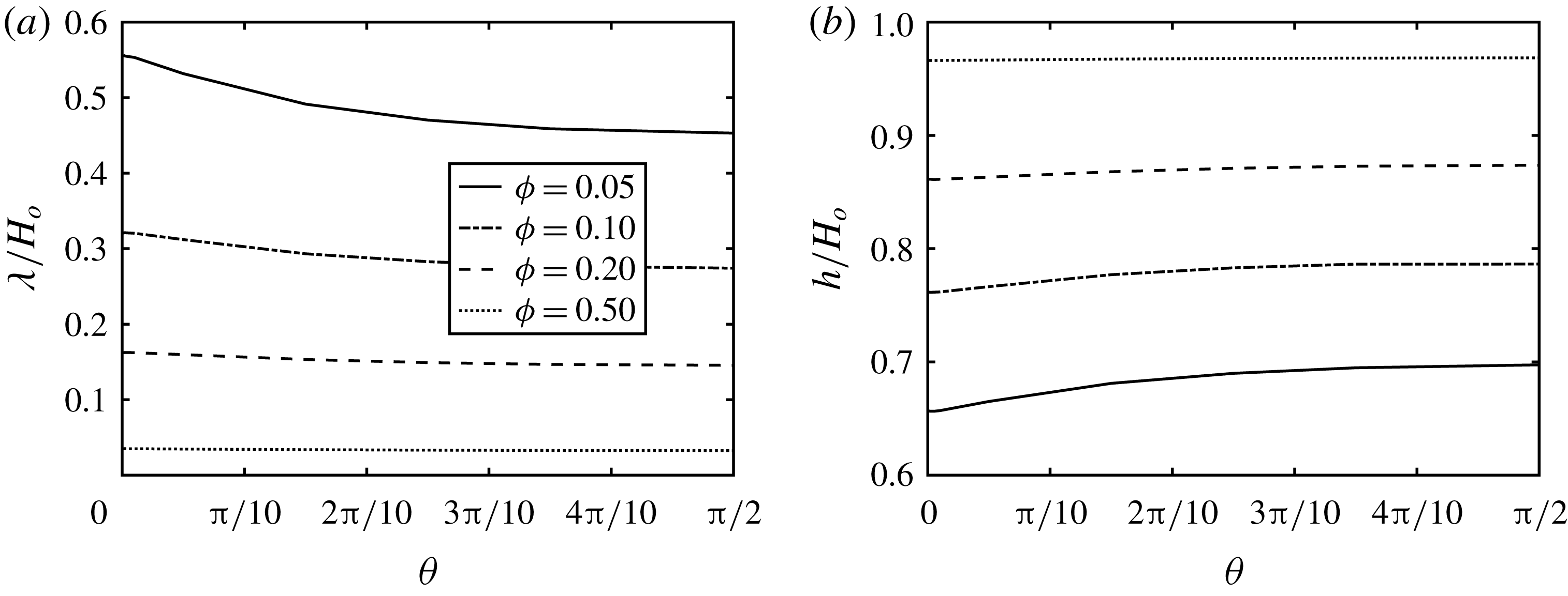
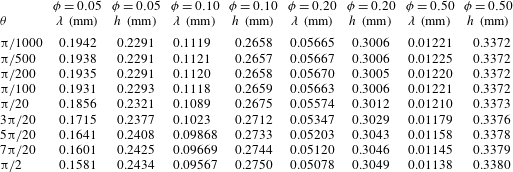
As for the macro-scale effect, figure 3 shows for several solid fractions $\unicode[STIX]{x1D719}$ that the normalized slip length slightly decreases and the film thickness increases from the peak to the equator. Clearly, a very small solid fraction leads to a very large slip length, hence very thin film and significant water repellency. Computed results are also shown in physical dimensions in table 2.

Figure 3.

Spatial variation of slip length and film thickness on the radome, normalized by the film thickness on a hydrophilic surface. Inputs are: $R=20~\text{m}$ , $\ell =0.18~\text{mm}$ , $d=0.0454~\text{mm}\;(\unicode[STIX]{x1D719}=0.05)$ , $0.0644~\text{mm}\;(\unicode[STIX]{x1D719}=0.10)$ and $0.0908~\text{mm}\;(\unicode[STIX]{x1D719}=0.20)$ .

Figure 4.

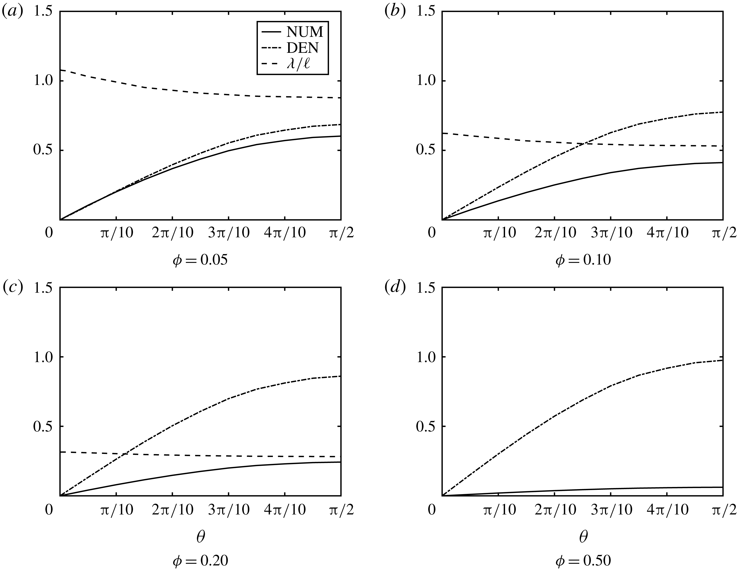
Radome with $R=20~\text{m}$ and different $\unicode[STIX]{x1D719}$ . Spatial variation of dimensionless slip length and parts of the fraction defining $\unicode[STIX]{x1D706}^{\prime }$ . NUM $=$  numerator of (2.29), DEN $=$  denominator of (2.29). For $\unicode[STIX]{x1D719}=0.50$ , $\unicode[STIX]{x1D706}^{\prime }\approx 0$ is too small to appear for the entire range of $\unicode[STIX]{x1D703}$ .

Table 2.

Slip length $\unicode[STIX]{x1D706}$ and film thickness $h$ on a radome: $R=20~\text{m}$ , $d=0.0454~\text{mm}$ , $Q=50~\text{mm}~\text{h}^{-1}$ , $H_{o}=0.349~\text{mm}$ .

A surprising result is that the slip length is finite near the radome peak where the mean flow and the shear rate reduce to zero, where their ratio should be ill defined. For a closer examination we show in figure 4 how the numerator and the denominator in (2.29) approach zero. It is their different gradients near the peak that renders their ratio and the slip length finite. As $\unicode[STIX]{x1D703}$ increases, both the numerator and denominator increase with the flow velocity. The denominator is always the larger for all solid fractions $\unicode[STIX]{x1D719}$ computed, but the contrast is most pronounced for the smallest $\unicode[STIX]{x1D719}$ , yielding the largest $\unicode[STIX]{x1D706}^{\prime }$ , as expected. As $\unicode[STIX]{x1D719}$ become large the numerator decreases much faster. The slip length ultimately diminishes to zero, signifying the loss of hydrophobicity.

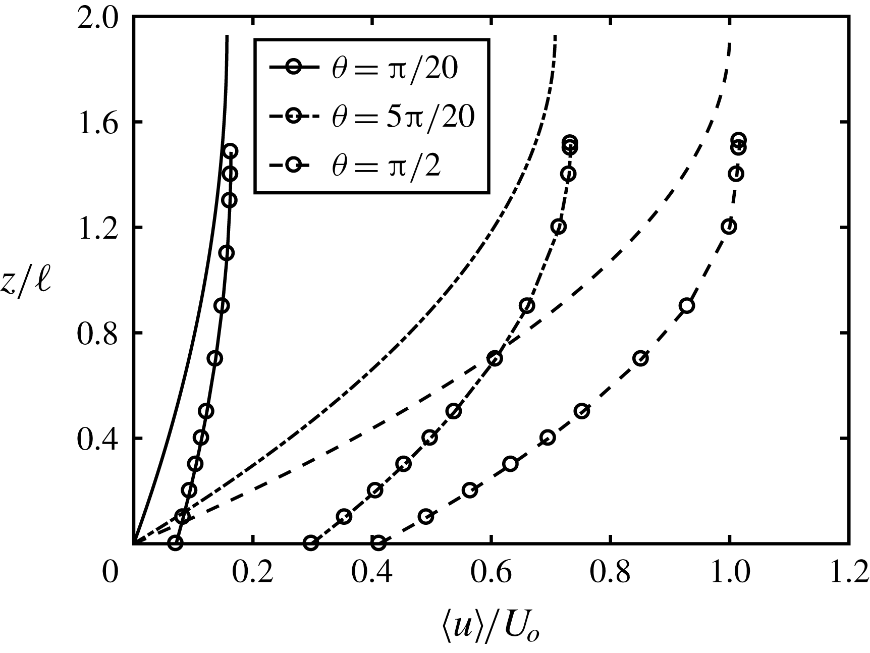
Finally figure 5 displays the depth profiles of velocity with finite slip at different $\unicode[STIX]{x1D703}$ over a hydrophobic radome for different $\unicode[STIX]{x1D719}$ . The maximum velocity in each profile occurs at the height corresponding to the local depth, which increases slightly with $\unicode[STIX]{x1D703}$ . For comparison the profiles in a film over a smooth hydrophilic surface are shown.

Figure 5.

Depth profiles of averaged cell velocity $\left\langle u\right\rangle$ at three angles. Inputs are: $R=20~\text{m}$ , $\ell =0.18~\text{mm}$ , $d=0.0644~\text{mm}\;(\unicode[STIX]{x1D719}=0.10)$ , $Re_{\ell }=55.4$ , $Q=50~\text{mm}~\text{h}^{-1}$ . Lines with circles: superhydrophobic radome. Lines: hydrophilic radome.

5 A roof top

Figure 6.

Roof top.

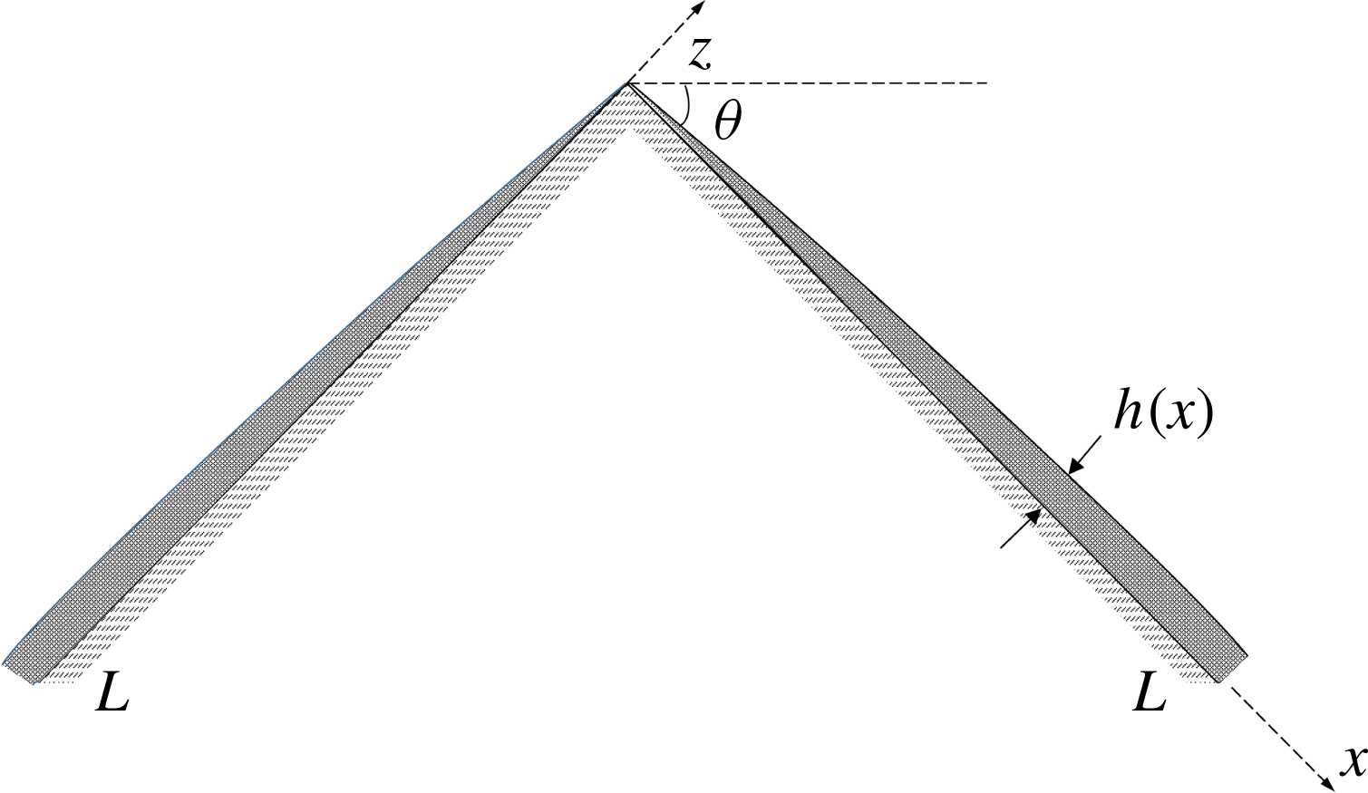
To examine the effect of the macro-scale geometry, let us consider the example of a roof top formed by two inclined planes joined at the peak. Each side is of length $L$ and inclined at an angle $\unicode[STIX]{x1D703}$ from the horizon, as shown in figure 6. Ignoring inertia, the mean flow velocity along the roof is formally the same as (2.5),

(5.1) $$\begin{eqnarray}u(x,z)=\frac{g}{\unicode[STIX]{x1D708}}\sin \unicode[STIX]{x1D703}\left(\unicode[STIX]{x1D706}h+hz-\frac{z^{2}}{2}\right);\quad 0<x<L,0<z<h,\end{eqnarray}$$

where $h(x)$ is to be found. The total volume outflux at any downstream station $x$ is

(5.2) $$\begin{eqnarray}\int _{0}^{h}\,\text{d}z\,u=\frac{g}{\unicode[STIX]{x1D708}}\left(\sin \unicode[STIX]{x1D703}\right)\left(\unicode[STIX]{x1D706}h^{2}+\frac{h^{3}}{3}\right).\end{eqnarray}$$

Equating the outflux to the total influx $Qx\cos \unicode[STIX]{x1D703}$ from the rain, we get

(5.3) $$\begin{eqnarray}h^{3}+3\unicode[STIX]{x1D706}h^{2}-\frac{Q\unicode[STIX]{x1D708}\cot \unicode[STIX]{x1D703}}{g}x=0.\end{eqnarray}$$

Let

(5.4) $$\begin{eqnarray}H=\left(\frac{Q\unicode[STIX]{x1D708}\cot \unicode[STIX]{x1D703}}{g}x\right)^{1/3}=H_{L}{X^{\prime }}^{1/3},\quad \text{i.e.},\;\frac{H}{H_{L}}={X^{\prime }}^{1/3},\end{eqnarray}$$

where

(5.5a,b ) $$\begin{eqnarray}H(L)\equiv H_{L}=\left(\frac{Q\unicode[STIX]{x1D708}\cot \unicode[STIX]{x1D703}}{g}L\right)^{1/3}\quad \text{and}\quad X^{\prime }=\frac{x}{L}.\end{eqnarray}$$

$H(X^{\prime })$ is now the variable film thickness on a hydrophilic roof top corresponding to $\unicode[STIX]{x1D706}=0$ , and $H_{L}$ is its value at the eave. Equation (5.3) becomes

(5.6) $$\begin{eqnarray}\frac{h^{3}}{H^{3}}+3\frac{\unicode[STIX]{x1D706}}{H}\frac{h^{2}}{H^{2}}-1=0,\end{eqnarray}$$

which gives $h$ for any $H(x)$ once $\unicode[STIX]{x1D706}(x)$ is found. Unlike the hemi-spherical dome, $H(x)$ replaces the constant $H_{0}$ and increases from zero at the roof peak $x=0$ monotonically to $H_{L}=H(L)$ at the eave $x=L$ .

The slip length and the new film thickness are found by a procedure similar to that for the radome. For brevity only the changes to the governing equations are summarized below. Adopting the same pillar array as for the radome, we modify the normalization of the micro-scale variables by replacing $H_{o}$ and $U_{o}$ in § 2 with $H_{L}$ and $U_{L}$ respectively, i.e.

(5.7a-c ) $$\begin{eqnarray}\boldsymbol{x}=\ell \boldsymbol{x}^{\prime },\quad \tilde{\boldsymbol{u}}=U_{L}\frac{\ell }{H_{L}}\tilde{\boldsymbol{u}}^{\prime },\quad \tilde{p}=\unicode[STIX]{x1D707}\frac{U_{L}}{\ell }\frac{\ell }{H_{L}}\tilde{p}^{\prime },\end{eqnarray}$$

where $U_{L}$ is the surface velocity at the downstream edge of the roof

(5.8) $$\begin{eqnarray}U_{L}=\frac{gH_{L}^{2}}{2\unicode[STIX]{x1D708}}\sin \unicode[STIX]{x1D703}=\frac{g^{1/3}}{2\unicode[STIX]{x1D708}^{1/3}}\left[Q\cot \unicode[STIX]{x1D703}L\right]^{2/3}\sin \unicode[STIX]{x1D703}.\end{eqnarray}$$

The basic flow on a smooth hydrophilic surface is now

(5.9) $$\begin{eqnarray}\displaystyle u_{B}(z,x)=U_{L}u_{B}^{\prime }(X^{\prime },z^{\prime }), & & \displaystyle\end{eqnarray}$$

where

(5.10) $$\begin{eqnarray}u_{B}^{\prime }(X^{\prime },z^{\prime })=2\frac{H^{2}}{H_{L}^{2}}\left(z^{\prime }\frac{\ell }{H}-{z^{\prime }}^{2}\frac{\ell ^{2}}{2H^{2}}\right).\end{eqnarray}$$

This result must be used in (2.25) to give the total local velocity (macro $+$ micro).

Equations (2.16) and (2.17) still hold formally for the perturbed flow in a typical cell above the bottom surface after replacing $U_{o}$ by $U_{L}$ and $H_{o}$ by $H_{L}$ and using (5.10) for $u_{B}^{\prime }$ and

(5.11) $$\begin{eqnarray}Re_{\ell }=\frac{U_{L}\ell }{\unicode[STIX]{x1D708}}\frac{\ell }{H_{L}}\end{eqnarray}$$

for the cell Reynolds number.

On the cell bottom, equation (2.21) must be changed to

(5.12) $$\begin{eqnarray}\frac{\unicode[STIX]{x2202}\tilde{u} ^{\prime }}{\unicode[STIX]{x2202}z^{\prime }}=-\left.\frac{H_{L}}{\ell }\frac{\unicode[STIX]{x2202}u_{B}^{\prime }}{\unicode[STIX]{x2202}z^{\prime }}\right|_{0}=-2\frac{H}{H_{L}}.\end{eqnarray}$$

On the cell top, $z^{\prime }=h^{\prime }=\ell h$ , equation (2.23) must be replaced by

(5.13) $$\begin{eqnarray}\frac{\unicode[STIX]{x2202}\tilde{u} ^{\prime }}{\unicode[STIX]{x2202}z^{\prime }}=-\left.\frac{H_{L}}{\ell }\frac{\unicode[STIX]{x2202}u_{B}^{\prime }}{\unicode[STIX]{x2202}z^{\prime }}\right|_{h^{\prime }}=-2\frac{H}{H_{L}}\left(1-h^{\prime }\frac{\ell }{H}\right).\end{eqnarray}$$

Other boundary conditions remain unchanged.

Figure 7.

Slip length and film thickness along the roof for four different solid fractions: (i) $d=0.0454~\text{mm}\;(\unicode[STIX]{x1D719}=0.05)$ , (ii) $d=0.0644~\text{mm}\;(\unicode[STIX]{x1D719}=0.10)$ , (iii) $d=0.0908~\text{mm}\;(\unicode[STIX]{x1D719}=0.20)$ , (iv) $d=0.1436~\text{mm}\;(\unicode[STIX]{x1D719}=0.50)$ . Inputs are: $L=10~\text{m}$ , $\unicode[STIX]{x1D703}=\unicode[STIX]{x03C0}/6$ , $\ell =0.18~\text{mm}$ . The layer depth $H(x)$ over a untextured surface is used for normalization.

After replacing $U_{o},H_{o}$ by $U_{L},H_{L}$ respectively, all equations for the area averaged flow from (2.25) onwards still hold. In particular the slip length $\unicode[STIX]{x1D706}^{\prime }=\unicode[STIX]{x1D706}/\ell$ is given by

(5.14) $$\begin{eqnarray}\unicode[STIX]{x1D706}^{\prime }(X^{\prime })=\left[\frac{(1-\unicode[STIX]{x1D719}){\displaystyle \frac{\ell }{H_{L}}}\left\langle \tilde{u} ^{\prime }\right\rangle _{f}}{\unicode[STIX]{x1D719}\left({\displaystyle \frac{\text{d}u_{B}^{\prime }}{\text{d}z^{\prime }}}+{\displaystyle \frac{\ell }{H_{L}}}\left\langle {\displaystyle \frac{\unicode[STIX]{x2202}\tilde{u} ^{\prime }}{\unicode[STIX]{x2202}z^{\prime }}}\right\rangle _{s}\right)}\right]_{0}.\end{eqnarray}$$

6 Numerical results for the roof top

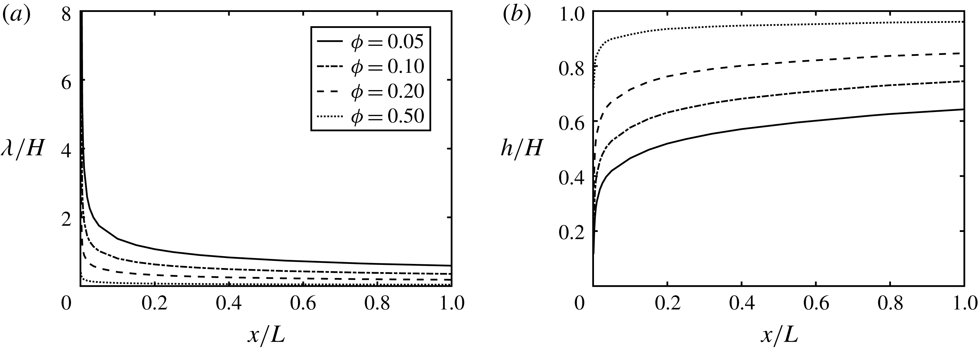
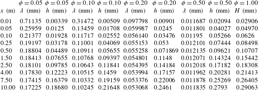
For demonstration we have chosen a roof of length $L=10~\text{m}$ , inclined at an angle of $30^{\circ }$ from the horizon. The rainfall intensity is $50~\text{mm}~\text{h}^{-1}$ . Figure 7 shows the variations of the normalized slip length and film thickness. Computed results are also shown in physical dimensions in table 3 where the normalizing thickness $H(x)$ on a smooth roof top is listed. For all $\unicode[STIX]{x1D719}$ , $\unicode[STIX]{x1D706}/H$ decreases from a large value at the peak then settles down to small values further down stream. Correspondingly $h/H$ increases with $X^{\prime }$ from 0 to a flat plateau. Results in physical dimensions are shown in table 3. These lengths are qualitatively different from those for a radome. For closer scrutiny, computations have been performed for the close neighbourhood of the peak near the radome top. In dimensional coordinates, the first cell is at $x=0.01~\text{m}$ very near the peak. For $\ell =0.18~\text{mm}$ and $\unicode[STIX]{x1D719}=0.1$ , we find $H(0.01~m)=0.02906~\text{mm}$ , and $h=0.00509~\text{mm}$ which is smaller than the pillar spacing $\ell$ . 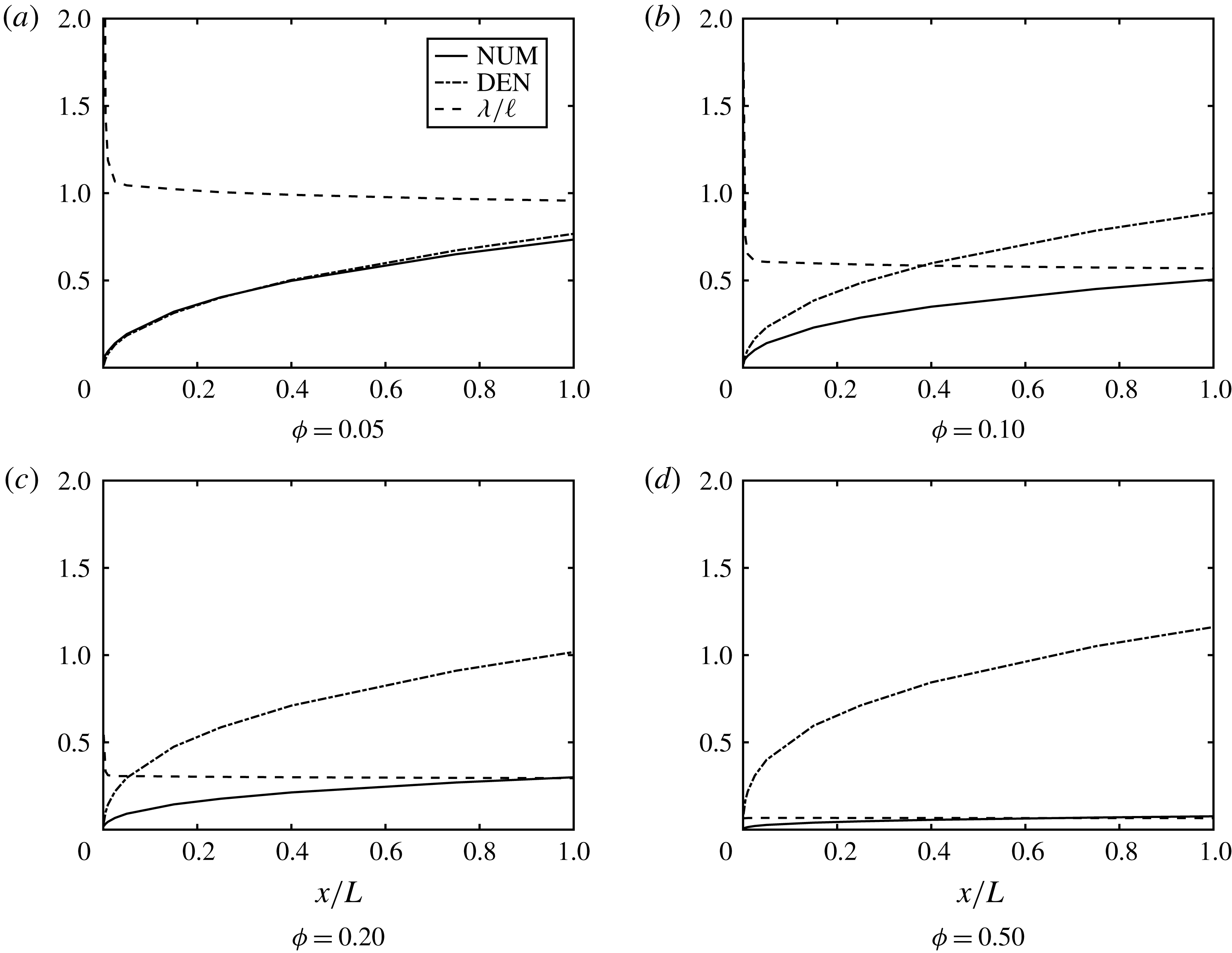Of course these results are of doubtful quantitative validity as the original assumptions of the length ratios no longer hold. To see the reason for this apparent singularity we plot in figure 8 various parts of the formula (5.14). For small $\unicode[STIX]{x1D719}$ , $(1-\unicode[STIX]{x1D719})\left\langle \tilde{u} ^{\prime }\right\rangle _{f}$ in the numerator quickly attains a non-zero value due to the finite roof slope (unlike the radome). In the denominator both $\unicode[STIX]{x1D719}(\unicode[STIX]{x2202}u_{B}^{\prime }/\unicode[STIX]{x2202}z^{\prime })\propto {X^{\prime }}^{1/3}$ and $\unicode[STIX]{x1D719}\left\langle \unicode[STIX]{x2202}\tilde{u} ^{\prime }/\unicode[STIX]{x2202}z^{\prime }\right\rangle _{s}$ are vanishingly small. This leads to the large ratio and the slip length.

Table 3.

Slip length and film thickness on a roof top; $L=10~\text{m}$ , $d=0.0454~\text{mm}$ , $Q=50~\text{mm}~\text{h}^{-1}$ . The last column gives the film thickness on a smooth untextured surface.

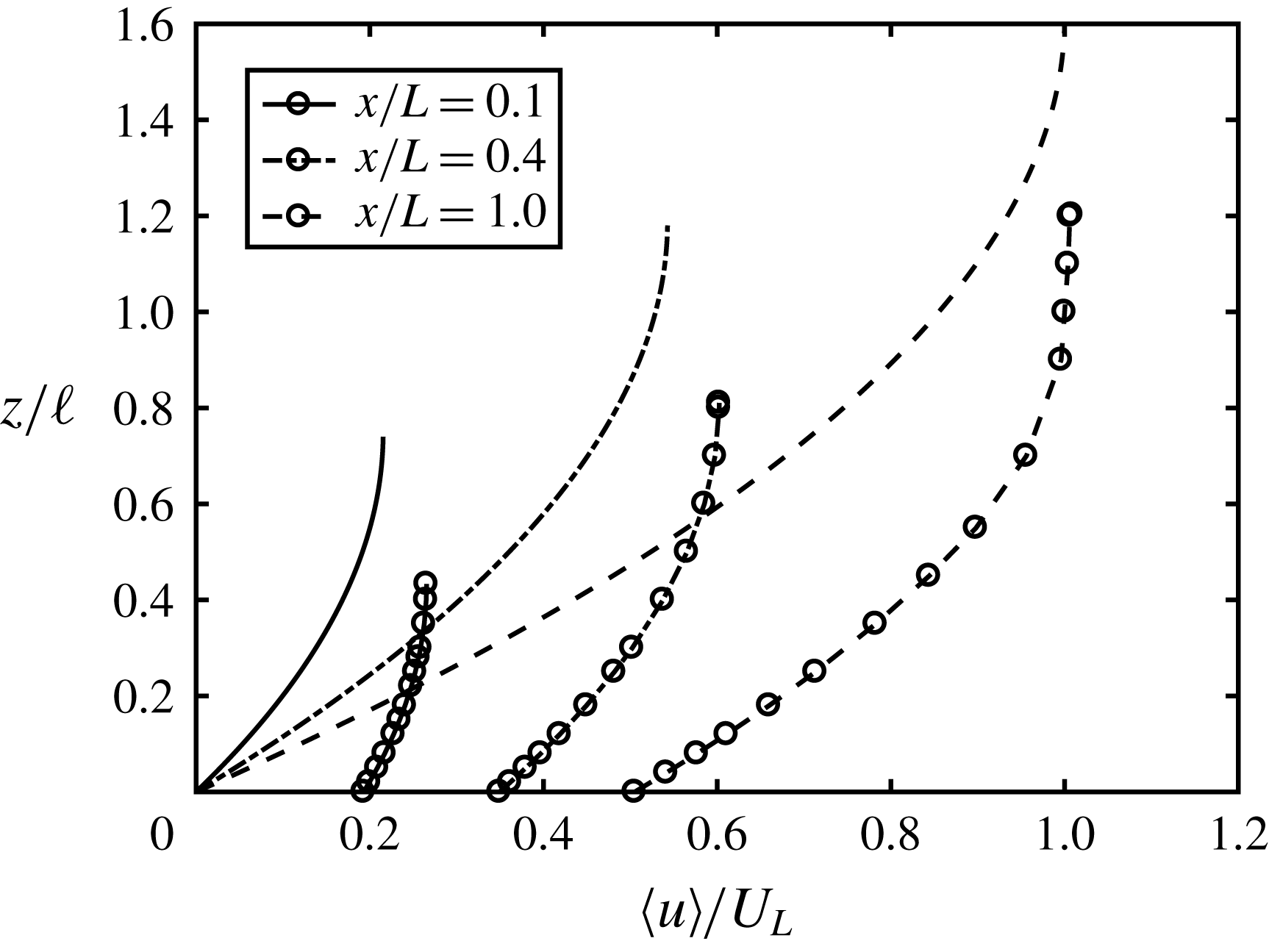
Finally figure 9 shows the depth profiles of the averaged velocity at three different stations on a roof. The increased slippage and thinning of the water film along the roof are obvious.

Figure 8.

Slip length along an inclined roof top. Inputs are the same as in figure 7. NUM $=$  numerator in (5.14). DEN $=$  denominator in (5.14).

Figure 9.

Depth profiles of averaged velocity at three stations of a roof with $\unicode[STIX]{x1D703}=\unicode[STIX]{x03C0}/6$ , $\unicode[STIX]{x1D719}=0.10$ , $L=10~\text{m}$ . Lines: smooth roof. Lines with circles: superhydrophobic roof.

7 Concluding remarks

A rainfall-induced water film on a radome surface is critical to the transmission loss of signals received by or radiated from a radar, and many studies have been devoted to the effectiveness of hydrophobic coatings for reducing the film thickness and signal degradation. In addition to empirical estimates, quantitative theories for the film flow should be valuable for guiding the design of coatings and reliable prediction of the radio-frequency waves. A semi-numerical theory is presented here for the slip length and film thickness on the macro-scale, based on a detailed analysis of the fluid mechanics on the micro-scale. Thanks to the sharp contrast of length scales, the numerical task of assessing the effects of many asperities can be reduced to the numerical solution of a limited number of cell problems. It is shown here that nonlinear convective inertia must be accounted for. However, each nonlinear cell problem can be solved with a modest effort by a standard finite element algorithm. After a small number of iterations the slip length and film thickness are determined. Numerical results are demonstrated for only a hemisphere and inclined planes on the macro-scale, and a square lattice of pillars on the micro-scale. Other geometries with regular arrays can be similarly treated and would be worthwhile. As many commercial coatings are random distributions of tiny particles of different sizes and shapes, a multiscale statistical theory including nonlinear inertia would be needed to reduce our reliance on empiricism. Thus far no measured data on the film thickness have been found in the published literature where attention is focussed solely on the transmission of EM waves. Direct experimental validation would be very worthwhile. Because of the usually large radome radius (10–20 m), field tests can likely be performed only by applying commercial hydrophobic coatings of random roughness. It is necessary to have reliable information of the hydrophobic properties such as the contact angle, roughness, etc. Accurate measurements of the local film thickness along different latitudes under a known rainfall rate must be made. For comparison with the present theory, the equivalent geometry of the lattice must be estimated. More precise experiments are possible in the laboratory for a small radome of $O(50)$  cm radius coated by a regular array of pillars (e.g. Choi et al. Reference Choi, Ulmanella, Kim, Ho and Kim2006). Details of local thickness and flow velocity over the entire surface can be measured under artificial rain.

Finally, as the length of high-frequency radio waves may be comparable to the film thickness (Blevis Reference Blevis1965), which is not always much greater in size than the asperities, scattering of EM waves by the asperities may warrant inclusion in future computations for hydrophobic radomes.