
1. Introduction
1.1. Dynamical systems approach for wall-bounded turbulence
Coherent structures in turbulent flows have been studied for many decades. These highly organised fluid motions in a chaotic flow field often carry a significant amount of turbulent kinetic energy and momentum. Understanding and modelling of their dynamics has been a central challenge in turbulence research. In wall-bounded shear flows, a coherent structure was first discovered in the near-wall region (Kline et al. Reference Kline, Reynolds, Schraub and Runstadler1967) and many different kinds of coherent structures were subsequently observed over the past half-century (e.g. Kovasznay, Kibens & Blackwelder (Reference Kovasznay, Kibens and Blackwelder1970), Falco (Reference Falco1977), Head & Bandyopadhay (Reference Head and Bandyopadhay1981), Jeong et al. (Reference Jeong, Benney, Schoppa and Kim1997), Kim & Adrian (Reference Kim and Adrian1999), del Álamo & Jiménez (Reference del Álamo and Jiménez2003), Hutchins & Marusic (Reference Hutchins and Marusic2007) and many others). The growing evidence suggests that these coherent structures are organised in the form of the so-called ‘attached eddies’ originally hypothesised by Townsend (Reference Townsend1956, Reference Townsend1976) for the logarithmic layer: coherent structures in the logarithmic layer emerge in the form of a self-similar hierarchy and their characteristic length scale is proportional to the distance between the eddy centre and the wall (see Hwang & Lee (Reference Hwang and Lee2020) for a mathematical proof). The attached eddy hypothesis can be extended to include the near-wall and outer regions in a broad sense (Hwang Reference Hwang2015), and there has been a growing body of evidence supporting this idea over the past decade (see the recent review of Marusic & Monty (Reference Marusic and Monty2019), and the references therein). In particular, each of these attached eddies was found to retain a sustaining mechanism independent of the others (Flores & Jiménez Reference Flores and Jiménez2010; Hwang & Cossu Reference Hwang and Cossu2010c, Reference Hwang and Cossu2011; Hwang & Bengana Reference Hwang and Bengana2016). This mechanism has been referred to as the ‘self-sustaining process’ (SSP) and is based on a quasi-cyclic interaction of streaks and quasi-streamwise vortices (Hamilton, Kim & Waleffe Reference Hamilton, Kim and Waleffe1995; Waleffe Reference Waleffe1997): (1) amplification of streamwise-elongated streaks by streamwise vortices through the lift-up effect (Butler & Farrell Reference Butler and Farrell1993; del Álamo & Jiménez Reference del Álamo and Jiménez2006; Cossu, Pujals & Depardon Reference Cossu, Pujals and Depardon2009; Hwang & Cossu Reference Hwang and Cossu2010a,Reference Hwang and Cossub); (2) breakdown of the amplified streaks via an instability and/or transient growth (Hamilton et al. Reference Hamilton, Kim and Waleffe1995; Schoppa & Hussain Reference Schoppa and Hussain2002; Park, Hwang & Cossu Reference Park, Hwang and Cossu2011; Alizard Reference Alizard2015; Cassinelli, de Giovanetti & Hwang Reference Cassinelli, de Giovanetti and Hwang2017; de Giovanetti, Sung & Hwang Reference de Giovanetti, Sung and Hwang2017; Lozano-Durán et al. Reference Lozano-Durán, Nikolaidis, Constantinou and Karp2021); (3) nonlinear regeneration of streamwise vortices (Hamilton et al. Reference Hamilton, Kim and Waleffe1995; Schoppa & Hussain Reference Schoppa and Hussain2002; Hwang & Bengana Reference Hwang and Bengana2016). A key ongoing challenge is to understand the interactions between the SSPs at multiple length scales, and recent studies have suggested that the interaction dynamics appear to be dauntingly complex (Cho, Hwang & Choi Reference Cho, Hwang and Choi2018; Lee & Moser Reference Lee and Moser2019; Doohan, Willis & Hwang Reference Doohan, Willis and Hwang2021).
The discovery of the SSP has played a central role in advancing the notions of dynamical systems for turbulence research. In particular, it physically underpins the existence of non-trivial unstable equilibrium and time-periodic solutions in wall-bounded shear flows (Nagata (Reference Nagata1990), Jiménez & Simens (Reference Jiménez and Simens2001), Kawahara & Kida (Reference Kawahara and Kida2001), Waleffe (Reference Waleffe2001), Waleffe (Reference Waleffe2003), Faisst & Eckhardt (Reference Faisst and Eckhardt2003), Wedin & Kerswell (Reference Wedin and Kerswell2004), Gibson, Halcrow & Cvitanovic (Reference Gibson, Halcrow and Cvitanovic2008), Gibson, Halcrow & Cvitanovic (Reference Gibson, Halcrow and Cvitanovic2009), Hall & Sherwin (Reference Hall and Sherwin2010), Park & Graham (Reference Park and Graham2015), Hwang, Willis & Cossu (Reference Hwang, Willis and Cossu2016) Doohan, Willis & Hwang (Reference Doohan, Willis and Hwang2019), Yang, Willis & Hwang (Reference Yang, Willis and Hwang2019) and many others). These solutions form a state-space skeleton for the birth of turbulence through a sequence of local and global bifurcations (Eckhardt et al. Reference Eckhardt, Schneider, Hof and Westerweel2007; Kawahara, Uhlmann & van Veen Reference Kawahara, Uhlmann and van Veen2012; Graham & Floryan Reference Graham and Floryan2020), and their use has been central to the description for the temporal dynamics of transition to turbulence (e.g. Kreilos & Eckhardt Reference Kreilos and Eckhardt2012) and for the local behaviour in the spatiotemporal dynamics (see the review by Barkley (Reference Barkley2016)). Furthermore, given that they are exact solutions to the Navier–Stokes equations, they provide precise understanding for turbulence dynamics in an interpretable and mathematically analysable manner especially compared with the structures obtained with conventional conditional average.
Despite these advances, the computation of the unstable equilibrium and periodic solutions are increasingly infeasible as the Reynolds number increases. A key reason for this is that the typical algorithms used for the search of these solutions are designed to iteratively find the initial condition that leads to the same flow field after a given time interval (an arbitrary small time interval for equilibrium and a time period for periodic orbits; e.g. Viswanath (Reference Viswanath2007), Willis, Cvitanovic & Avila (Reference Willis, Cvitanovic and Avila2013) and Farazmand (Reference Farazmand2016)). Apart from the computational cost required for the repeated simulations, the numerical convergence of such an algorithm depends on the leading Lyapunov exponent of the related chaotic state – it becomes increasingly difficult to find an initial flow field which converges with a sufficiently small residual when the leading Lyapunov exponent is very large. An approach employed to bypass this difficulty was to approximate the complex multiscale dynamics at high Reynolds numbers with a closure model (e.g. Rawat et al. Reference Rawat, Cossu, Hwang and Rincon2015; Hwang et al. Reference Hwang, Willis and Cossu2016; Yang et al. Reference Yang, Willis and Hwang2019). Yet, the unstable equilibrium and periodic solutions obtained with this strategy are often obtained by continuing the existing solutions at low Reynolds numbers, thereby not retaining the key multiscale processes of interest at high Reynolds numbers (e.g. scale interactions). Indeed, a very recent work by Doohan et al. (Reference Doohan, Bengana, Yang, Willis and Hwang2022) showed that when turbulence exhibits multiscale behaviours explicitly, most of the equilibrium solutions obtained in this manner do not sit anywhere near the turbulent state in the physically relevant phase portraits. An obvious way to resolve this issue is to compute unstable periodic orbits with sufficiently long time periods, as they should be able to capture the key periodic and/or quasi-periodic multiscale dynamics. However, in practice, their computation is much more difficult than that of the equilibrium solutions and is practically almost impossible due to the rapidly vanishing convergence of the solutions by the increasing Reynolds number. This poses an important challenge in extending the notions of dynamical systems for the description of multiscale behaviours of turbulent flows.
Given this challenge, it is worth mentioning that many of the unstable equilibria and periodic solutions have previously been computed in a highly reduced system even at low Reynolds numbers. Indeed, a large number of such solutions have been found in highly confined computational domains, in which the full spatiotemporal dynamics in a large computational domain would be drastically reduced (Nagata Reference Nagata1990; Waleffe Reference Waleffe1995; Jiménez & Simens Reference Jiménez and Simens2001; Kawahara & Kida Reference Kawahara and Kida2001; Faisst & Eckhardt Reference Faisst and Eckhardt2003; Wedin & Kerswell Reference Wedin and Kerswell2004; Gibson et al. Reference Gibson, Halcrow and Cvitanovic2008; Park & Graham Reference Park and Graham2015; Hwang et al. Reference Hwang, Willis and Cossu2016; Doohan et al. Reference Doohan, Willis and Hwang2019, Reference Doohan, Bengana, Yang, Willis and Hwang2022). For the same rationale, perhaps, the key to tackling the multiscale dynamics of turbulence using the dynamical systems notions may lie in a suitable dimensionality reduction of the given turbulent state without losing the core dynamics of interest. The equilibrium and periodic solutions to the reduced-order dynamical system can then be obtained much more easily using existing techniques, with hope that they can subsequently be used as proxies and/or a symbolic description for the multiscale dynamics of a turbulent system.
1.2. Reduced-order modelling
Reduced-order modelling has been a long-standing topic in fluid mechanics, and wall-bounded turbulence is a flow configuration to which the earliest modelling efforts were made (Aubry et al. Reference Aubry, Holmes, Lumley and Stone1988; Rempfer & Fasel Reference Rempfer and Fasel1994a). The previous efforts may be classified into two categories. One is based on the POD (e.g. Lumley Reference Lumley1967, Reference Lumley1981; Sirovich Reference Sirovich1987; Holmes, Lumley & Berkooz Reference Holmes, Lumley and Berkooz1996), and the reduced-order model is subsequently obtained by projecting the Navier–Stokes equations onto the space spanned by the proper orthogonal decomposition (POD) modes (i.e. Galerkin projection; Aubry et al. Reference Aubry, Holmes, Lumley and Stone1988; Rempfer & Fasel Reference Rempfer and Fasel1994a,Reference Rempfer and Faselb; Smith, Moehlis & Holmes Reference Smith, Moehlis and Holmes2005). The other is equivalent to a heavily truncated spectral approximation to the system of interest (Waleffe Reference Waleffe1997; Moehlis, Faisst & Eckhardt Reference Moehlis, Faisst and Eckhardt2004, Reference Moehlis, Faisst and Eckhardt2005; Lagha & Manneville Reference Lagha and Manneville2007; Chantry, Tuckerman & Barkley Reference Chantry, Tuckerman and Barkley2017; Cavalieri Reference Cavalieri2021), which is often used to study low-dimensional dynamics of bifurcation and transition to turbulence. Given the scope of the present study, here we shall employ the former approach based on POD modes, as they provide the best orthonormal basis in terms of capturing the energy of the given flow fields.
One of the key challenges in the development of a reduced-order model using the POD modes is often associated with the number of POD modes considered and the resulting truncation. This problem becomes significant especially for high Reynolds number flows, where the small-scale motions, not captured by the chosen POD modes, play a crucial role in the energy cascade and turbulent dissipation. Indeed, one of the most fundamental features of turbulence is the exact balance between the production at large scale and the dissipation at the small (Kolmogorov) scale. Therefore, not accounting for such small-scale motions leads to an excess of energy and/or an erroneous behaviour in the reduced-order model. This issue has often been resolved by incorporating an additional eddy-viscosity model that removes the excess in the energy of the reduced-order model (Aubry et al. Reference Aubry, Holmes, Lumley and Stone1988; Rempfer & Fasel Reference Rempfer and Fasel1994b; Couplet, Basdevant & Sagaut Reference Couplet, Basdevant and Sagaut2005; Smith et al. Reference Smith, Moehlis and Holmes2005; Noack, Morzýnski & Tadmor Reference Noack, Morzýnski and Tadmor2011; Östh et al. Reference Östh, Noack, Krajnović, Barros and Borée2014; Protas, Noack & Östh Reference Protas, Noack and Östh2015). Given the scope of the present study, the approach of Protas et al. (Reference Protas, Noack and Östh2015) is particularly appealing, in which an ‘optimal’ eddy viscosity was proposed to minimise the difference between the data from the measurement and from the reduced-order model. In this approach, the gradient of the given objective functional is computed over multiple time intervals using the adjoint-based formulation. The best-performing eddy viscosity is subsequently obtained by updating its value at every time interval, an approach reminiscent of the ‘suboptimal’ control in the flow control problem (Choi et al. Reference Choi, Temam, Moin and Kim1993; Lee, Kim & Choi Reference Lee, Kim and Choi1999). It is worth mentioning that such an optimisation problem is ideally formulated with an objective functional considering a long time interval. However, the resulting adjoint equation for the Lagrange multiplier is mathematically unstable around the chaotic trajectory due to the positive leading Lyapunov exponent. This inherently limits the size of the time interval that can be used for the gradient calculation. Furthermore, the leading Lyapunov exponent rapidly grows with the Reynolds number, forming an important challenge in the application of such an approach for high Reynolds numbers – indeed, a similar issue of the time interval in the adjoint-based optimisation problem was previously discussed in the context of an optimal control problem (e.g. Bewley, Moin & Temam Reference Bewley, Moin and Temam2001). Recently, there have been a rapidly growing number of studies aiming to identify the governing dynamics solely from simulation and experimental data available (e.g. Schmidt & Lipson Reference Schmidt and Lipson2009; Brunton, Proctor & Kutz Reference Brunton, Proctor and Kutz2016; Loiseau & Brunton Reference Loiseau and Brunton2018). In the context of fluid mechanics, a novel approach was proposed by Brunton et al. (Reference Brunton, Proctor and Kutz2016), who accurately identified the governing low-dimensional dynamics of Lorenz chaos and the two-dimensional laminar cylinder wake from data. In their study, a reduced-order model based on POD modes is identified in a data-driven manner by formulating an  $l_1$-regularisation-based optimisation which minimises the difference between the full and the reduced-order dynamics – the approach referred to as ‘sparse identification of nonlinear dynamics’ (SINDy). Furthermore, the SINDy framework has been extended by Loiseau & Brunton (Reference Loiseau and Brunton2018), who introduced a constraint enforcing energy-preserving nonlinearity by reformulating the sparse regression problem with the Karush–Kuhn–Tucker conditions. There is also ongoing effort to improve low-dimensional representation of nonlinear dynamics by nonlinear correlations in the temporal POD coefficients (Callaham, Brunton & Loiseau Reference Callaham, Brunton and Loiseau2021a). For high Reynolds number turbulent flows, a recent study by Callaham et al. (Reference Callaham, Loiseau, Rigas and Brunton2021b), the statistical-state dynamics of turbulence in three-dimensional bluff-body wake was modelled by combining a normal form amplitude equation with stochastic noise determined using a similar sparse regression. This approach based on a simple normal form amplitude equation is, however, not attractive for wall-bounded shear flows, as the key coherent structure dynamics in this case involves a much more sophisticated global bifurcation (e.g. the crisis bifurcation; see Kreilos & Eckhardt (Reference Kreilos and Eckhardt2012)) as well as a rich spatiotemporal dynamics that can be described with the concept of thermodynamic phase transition (e.g. Avila et al. Reference Avila, Moxey, de Lozar, Avila, Barkley and Hof2011; Barkley Reference Barkley2016). It is finally worth mentioning that, in the context of turbulence modelling, there have been several successful recent efforts made with the use of SINDy for a closure of the Reynolds-averaged Navier–Stokes equations (e.g. Beetham & Capecelatro Reference Beetham and Capecelatro2020; Schmelzer, Dwight & Cinnella Reference Schmelzer, Dwight and Cinnella2020; Beetham, Fox & Capecelatro Reference Beetham, Fox and Capecelatro2021). A comprehensive review on the utilisation of machine learning approaches for turbulence modelling in Reynolds-averaged Navier–Stokes and large eddy simulation can also be found in Duraisamy (Reference Duraisamy2021), where the need to augment the given turbulent model using machine learning methods with suitable physical constraints was discussed.
1.3. Objective of the present study
The objective of the present study is to develop a reduced-order model which is more accurate than conventional ones for a turbulent state in wall-bounded shear flows. As the first step towards this task, we will consider a relatively simple but turbulent system; i.e. the minimal flow unit of a plane Couette flow (PCF) (Hamilton et al. Reference Hamilton, Kim and Waleffe1995), where the chaotic dynamics is well described in terms of the SSP. Based on the utilisation of POD modes, four different approaches will be considered and compared to devise a best performing reduced-order model: (1) Galerkin projection with a simple truncation; (2) sparse Galerkin regression (i.e. application of SINDy (Brunton et al. Reference Brunton, Proctor and Kutz2016)); (3) Galerkin projection with a simple eddy-viscosity closure (Smith et al. Reference Smith, Moehlis and Holmes2005); (4) Galerkin projection with a SINDy closure for the truncation error. In particular, the last approach mentioned here is new and is proposed by the present study, in which the concept of the optimal eddy viscosity (Protas et al. Reference Protas, Noack and Östh2015) will be combined with a sparse regression. The idea of calibration of a given reduced-order model with an eddy-viscosity closure was previously proposed by several studies (e.g. Couplet et al. Reference Couplet, Basdevant and Sagaut2005; Cordier, El Majd & Favier Reference Cordier, El Majd and Favier2010) with different types of regularisations. A similar idea was also recently explored in the recent work by Mohebujjaman, Rebholz & Iliescu (Reference Mohebujjaman, Rebholz and Iliescu2019), who applied a data-driven correction to a two-dimensional cylinder flow without an explicit physical closure model. In this context, it is worth mentioning that an important benefit of the  $l_1$-regularisation used in this study over the common
 $l_2$-regularisation is that it prevents possible overfit of the eddy viscosity model which might yield an overdamped reduced-order model. The
 $l_1$-regularisation will also offer a more parsimonious low-dimensional description. We will see that this approach enables us to effectively determine an ‘optimal’ eddy viscosity, significantly improving the accuracy of the low-dimensional model based on POD modes.
This paper is organised as follows. In § 2, the equations of motion, the flow geometry and the POD modes are introduced. The four reduced-order models are subsequently introduced and formulated in § 3 and their performance will be examined and mutually compared in § 4. This paper concludes in § 5.
2. Background
2.1. PCF
We consider a PCF of an incompressible fluid, where the two walls move in opposite directions with streamwise velocity,  ${\pm }U_w$. The wall-normal distance between the two walls is given by
 $2h$. The kinematic viscosity of the fluid is
 $\nu$, and the Reynolds number is defined by
 $Re = U_w h/\nu$. The streamwise, wall-normal and spanwise coordinates are made dimensionless with
 $h$, and they are denoted by
 $\boldsymbol {x} = (x,y,z)$. The two walls are set to be located at
 $y=\pm 1$. The equations of motion are then given by
 \begin{equation} \frac{\partial \boldsymbol{u}}{\partial t} ={-}(\boldsymbol{u} \boldsymbol{\cdot} \boldsymbol{\nabla}) \boldsymbol{u} - y\frac{\partial \boldsymbol{u}}{\partial x} - {v} \boldsymbol{e}_x - \boldsymbol{\nabla} p + \frac{1}{Re}\nabla^{2}\boldsymbol{u}, \end{equation}
where  $t$ is the time,
 $\boldsymbol {u}=({u},{v},{w})$ is the perturbation velocity from the laminar base flow,
 $\boldsymbol {U}=(y,0,0)$,
 $p$ the pressure and
 $\boldsymbol {e}_x$ the unit vector in the streamwise direction.
To build a reduced-order model, we first perform a direct numerical simulation (DNS) confined to a minimal flow unit (Jiménez & Moin Reference Jiménez and Moin1991; Hamilton et al. Reference Hamilton, Kim and Waleffe1995). Following Hamilton et al. (Reference Hamilton, Kim and Waleffe1995), the computational domain of  $(L_x,L_y,L_z)=(1.75{\rm \pi},2,1.2{\rm \pi} )$ is considered at
 $Re=400$. The simulation was performed using channelflow 2.0, an open-source DNS code (https://www.channelflow.ch/). The code uses the Fourier–Galerkin discretisation in the streamwise and spanwise directions and the Chebyshev-tau discretisation in the wall-normal direction. The number of grid points in each spatial direction is given by (
 $N_x,N_y,N_z) = (16,33,16$) (after dealiasing). A third-order semi-implicit backward difference formula (SDBF3) is used for the time-integration scheme. The simulation has been performed by setting a zero pressure gradient. The domain size normalised by viscous inner units (denoted by the superscript
 $(\cdot )^{+}$) is obtained as
 $(L_x^{+},{L_y^{+}},L_z^{+}) \simeq (186,68,127)$, in good agreement with that in Hamilton et al. (Reference Hamilton, Kim and Waleffe1995).
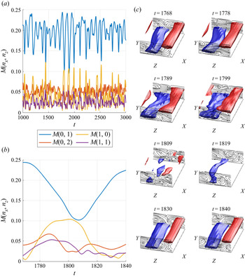
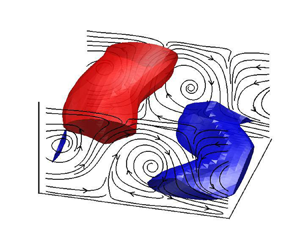
Figure 1 shows the DNS results, which exhibit the SSP. To examine the time evolution of the flow fields, the square root of energy of each plane Fourier mode is introduced,
 \begin{equation} M(n_x,n_z) = \left(\int_{{-}1}^{1} [\hat{{u}}^{2}(n_x,n_z,y) + \hat{{v}}^{2}(n_x,n_z,y) + \hat{{w}}^{2}(n_x,n_z,y)] \,\mathrm{d} y\right)^{{1}/{2}}, \end{equation}
where  $(\hat {\cdot })$ denotes the Fourier coefficients for the perturbation velocity, and
 $n_x$ and
 $n_z$ define the streamwise and spanwise wavenumbers such that
 $n_x \alpha$ and
 $n_z \beta$ (
 $\alpha = 2{\rm \pi} /L_x$ and
 $\beta = 2{\rm \pi} /L_z$). Figure 1(a) shows the time trace featuring the quasi-periodic oscillation at the SSP time scale,
 $T_{SSP} \approx 80\text {--}90$. A sequence of flow field snapshots for a single SSP cycle, which correspond to the time trace in figure 1(b), are shown in figure 1(c). The initial flow field is featured with an amplified state of the high- and low-speed streamwise velocity streaks (
 $t=1768$) (note that the time evolution of the streaks is depicted by
 $M(0,1)$ in figure 1b). The streaks subsequently become unstable (Hamilton et al. Reference Hamilton, Kim and Waleffe1995) or experience the related transient growth (Schoppa & Hussain Reference Schoppa and Hussain2002), leading to their breakdown in a sinuously meandering manner. The streak breakdown emerges at
 $t=1809$ where the streaks evidently disappear. Nonlinear processes subsequently regenerate streamwise vortices, leading to an increase in
 $M(1,1)$. Finally, for
 $t=1819\text {--}1840$, the regenerated streamwise vortices (
 $y$–
 $z$ cut planes) redistribute the momentum from mean shear, resulting in the formation of new streaks especially near the lower wall region. This mechanism is known as the ‘lift-up’ effect.
Time trace of  $M(0,1)$,
 $M(0,2)$,
 $M(1,0)$,
 $M(1,1)$ (a) for
 $t=1000\text {--}3000$ and (b) for
 $t=1768\text {--}1840$. (c) Flow snapshots at
 $t=1768, 1778, 1789, 1799, 1809, 1819, 1830, 1840$, where the blue and red isosurfaces indicate
 $u={\pm }0.65$, respectively.

2.2. POD
The POD seeks a set of orthonormal functions that maximises the ensemble-averaged projection of the velocity perturbation,  $\boldsymbol {u}$ (e.g. Holmes et al. Reference Holmes, Lumley and Berkooz1996). The optimisation is performed by solving the following eigenvalue problem:
 \begin{equation} \int_{\varOmega} \left\langle{\boldsymbol{u}(\boldsymbol{x},t)\boldsymbol{u}^{H}(\boldsymbol{x'},t)}\right\rangle \boldsymbol{\varPhi}_{n_x,n_z}^{(n)}(\boldsymbol{x'})\, {\rm d}^{3}\boldsymbol{x'} = \lambda_{n_x,n_z}^{(n)}\boldsymbol{\varPhi}_{n_x,n_z}^{(n)}(\boldsymbol{x}), \end{equation}
where  $(\cdot )^{H}$ is the complex conjugate transpose,
 $\left\langle {\cdot }\right\rangle $ an ensemble average,
 $\lambda _{n_x,n_z}^{(n)}$, the eigenvalue representing the average kinetic energy contained in each POD mode and
 $\boldsymbol {\varPhi }_{n_x,n_z}^{(n)}$ are the POD modes. Here, the eigenvalue and the corresponding POD modes are indexed by a positive integer
 $n$ in decreasing order of the eigenvalue for each pair of the streamwise and spanwise wavenumber indices,
 $(n_x, n_z)$. The perturbation velocities are then represented in terms of a linear superposition of the POD modes,
 \begin{equation} \boldsymbol{u}(\boldsymbol{x},t) = \sum_{n_x={-}\infty}^{\infty}\sum_{n_z={-}\infty}^{\infty}\sum_{n=1}^{\infty} a_{n_x,n_z}^{(n)} (t) \boldsymbol{\varPhi}_{n_x,n_z}^{(n)}(\boldsymbol{x}), \end{equation}
where  $a_{n_x,n_z}^{(n)}(t)$ is the time-dependent amplitude of each POD mode. Given the translational invariance in the streamwise and spanwise directions, Fourier expansions are optimal and the POD mode is further written as
 \begin{equation} \boldsymbol{\varPhi}_{n_x,n_z}^{(n)}(\boldsymbol{x}) = \frac{1}{\sqrt{L_xL_z}} \exp({{\rm i}(\alpha n_x x+\beta n_z z)}) \boldsymbol{\phi}_{n_x,n_z}^{(n)}(y), \end{equation}
where  $\boldsymbol {\phi }_{n_x,n_z}^{(n)}(y)$ describes the wall-normal structure of each POD mode. Since the velocities in physical space are real valued, the following conjugate symmetries are also satisfied:
 \begin{equation} a_{n_x,n_z}^{(n)}(t) = a_{{-}n_x,-n_z}^{(n)*}(t) \quad \textrm{and} \quad \boldsymbol{\varPhi}_{n_x,n_z}^{(n)} = \boldsymbol{\varPhi}_{{-}n_x,-n_z}^{(n)*}, \end{equation}
where the superscript  $(\cdot )^{*}$ indicates the complex conjugate. Substituting (2.4a) and (2.4b) into (2.3), the eigenvalue problem is simplified to
 \begin{equation} \int_{{-}1}^{1} \underbrace{\left\langle{\hat{\boldsymbol{u}}(n_x,n_z,y,t)\hat{\boldsymbol{u}}^{H}(n_x,n_z,y',t)}\right\rangle}_{{\equiv} \hat{\boldsymbol{R}}}\boldsymbol{\phi}_{n_x,n_z}^{(n)}(y') \,\mathrm{d} y' = \lambda_{n_x,n_z}^{(n)}\boldsymbol{\phi}_{n_x,n_z}^{(n)}(y). \end{equation}
The ensemble-averaged covariance  $\hat {\boldsymbol {R}}$ is computed by enforcing the discrete symmetries of the PCF,
 \begin{equation} \left.\begin{gathered} \mathcal{I}:[{u},{v},{w},p](x,y,z,t) = [{u},{v},{w} ,p](x,y,z,t),\\ \mathcal{P}:[{u},{v},{w},p](x,y,z,t) = [{-u},{-v},{-w}, p]({-}x,-y,-z,t),\\ \mathcal{R}:[{u},{v},{w},p](x,y,z,t) = [{u},{v},{-w}, p](x,y,-z,t),\\ \mathcal{R} \mathcal{P}:[{u},{v},{w},p](x,y,z,t) = [{-u},{-v},{w}, p]({-}x,-y,z,t), \end{gathered}\right\} \end{equation}
where  $\mathcal {I}$ is the identify transformation,
 $\mathcal {P}$ is a point reflection about the origin,
 $\mathcal {R}$ is a reflection about the
 $z$-plane and
 $\mathcal {RP}$ is a
 $180^{\circ }$ rotation about the
 $z$-axis. Given the statistically stationary nature of the turbulent state and the invariance of the PCF under the discrete group transformation in (2.6), the covariance operator is obtained as
 \begin{equation} \hat{\boldsymbol{R}}(n_x,n_z,y,y')=\frac{1}{4T} \int_{t_0}^{t_0+T} \sum_{\mathcal{T}\in \mathcal{D}_2}(\widehat{\mathcal{T}:{\boldsymbol{u}}})(n_x,n_z,y,t)(\widehat{\mathcal{T}:{\boldsymbol{u}}})^{H}(n_x,n_z,y',t) \,\mathrm{d}t, \end{equation}
where  $\mathcal {D}_2 = \{\mathcal {I},\mathcal {P},\mathcal {R},\mathcal {RP}\}$.
For the computation of the POD modes, the ensemble-averaged covariance  $\hat {\boldsymbol {R}}$ is first obtained and the eigenvalue problem (2.5) is subsequently solved. Since the ensemble average is equivalent to the time average for a statistically stationary flow,
 $\hat {\boldsymbol {R}}$ is obtained by averaging in time over an interval
 $t \in [-10\,000,0]$ with a sampling time interval
 $\Delta t=1$ (i.e.
 $t_0=-10\,000$ and
 $T=10\,000$). Within this time interval, the turbulent state is chosen to be statistically stationary. We also note that the typical time period of the SSP is approximately
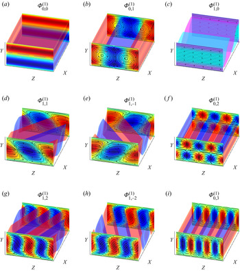
 $T_{SSP} \approx 80\text{--} 90$, implying that more than 100 cycles are considered for the construction of the POD modes. Table 1 shows the leading eigenvalues obtained in the present study, and they are found to match closely with those reported in Smith et al. (Reference Smith, Moehlis and Holmes2005). The structures of the nine leading POD modes are also visualised in figure 2.
Eigenvalues of the first seven POD modes, ranked in terms of the eigenvalue of the POD mode  $\lambda$. Here,
 $E \, [\%]$ is the total energy content of both
 $(n_x,n_z,n)$ and
 $(-n_x,-n_z,n)$ wavenumber pairs.

Visualisation of nine leading POD modes  $(n_x,n_z,n)$: (a)
 $(0,0,1)$; (b)
 $(0,1,1)$; (c)
 $(1,0,1)$; (d)
 $(1,1,1)$; (e)
 $(1,-1,1)$; ( f)
 $(0,2,1)$; (g)
 $(1,2,1)$; (h)
 $(1,-2,1)$; (i)
 $(0,3,1)$. Isosurfaces of (a,b,d–i) denote
 $u = -0.15$ (red) and
 $u= 0.15$ (blue). Isosurfaces of (c) denote
 $w = 0.15$ (teal) and
 $w=-0.15$ (purple).

3. Reduced-order models
3.1. POD-Galerkin projection
To build a reduced-order model, we consider the velocity given by (2.4a) with a finite number of POD modes,
 \begin{equation} \boldsymbol{u}(\boldsymbol{x},t) = \sum_{n_x={-}M_x}^{M_x}\sum_{n_z={-}M_z}^{M_z}\sum_{n=1}^{N_p} a_{n_x,n_z}^{(n)} (t) \boldsymbol{\varPhi}_{n_x,n_z}^{(n)}(\boldsymbol{x}) + \boldsymbol{u}_R(\boldsymbol{x},t), \end{equation}
where  $M_x$,
 $M_z$ and
 $N_p$ are the numbers of streamwise Fourier modes, spanwise Fourier modes and
 $\boldsymbol {\phi }_{n_x,n_z}^{(n)}$, respectively. Here
 $\boldsymbol {u}_R(\boldsymbol {x},t)$ is the residual velocity field that will not be resolved by the reduced-order model. After substituting (3.1) into (2.1), the projection onto each POD basis yields the following system of ordinary different equations:
 \begin{equation} \dot{\boldsymbol{a}} = \boldsymbol{L} \boldsymbol{a} +\boldsymbol{N}(\boldsymbol{a},\boldsymbol{a})+\boldsymbol{T}, \end{equation}
where  $\dot {(\cdot )}\equiv \textrm {d}/\textrm {d}t$,
 $\boldsymbol {a} \in \mathbb {C}^{r}$ with
 $r = [(2M_x + 1)(2M_z+1)N_P+1]/2$ as the column vector, the element of which is given by
 $a_{n_x,n_z}^{(n)}$ for
 $-M_x \leqslant n_x \leqslant M_x$,
 $-M_z \leqslant n_z \leqslant M_z$ and
 $1 \leqslant n \leqslant N_p$,
 $\boldsymbol {L}$ and
 $\boldsymbol {N}$ are from the projection of the linear and quadratic nonlinear parts of (2.1) onto the finite number of POD modes (for further details on their definitions, see Appendix A), and
 $\boldsymbol {T}$ is the residual term originating from
 $\boldsymbol {u}_R(\boldsymbol {x},t)$. From (3.2), the simplest low-dimensional model is obtained by ignoring the residual term, i.e.
 \begin{equation} \boldsymbol{T}=\boldsymbol{0}. \end{equation}
This case shall be referred to as the POD-Galerkin model.
3.2. Sparse POD-Galerkin regression
Several recent studies have been proposed to identify  $\boldsymbol {L}$ and
 $\boldsymbol {N}$ directly from the data (Brunton et al. Reference Brunton, Proctor and Kutz2016; Loiseau & Brunton Reference Loiseau and Brunton2018). If the dimension of the given nonlinear oscillation is sufficiently low (e.g. two-dimensional laminar cylinder wake),
 $\boldsymbol {T}$ can be ignored with the use of a small number of POD modes. In this case,
 $\boldsymbol {L}$ and
 $\boldsymbol {N}$ can directly be obtained from the snapshots of
 $\boldsymbol {a}$ using a sparse regression technique (i.e. SINDy; e.g. Brunton et al. (Reference Brunton, Proctor and Kutz2016)). Now, SINDy is formulated by first collecting a set of time snapshots of the POD amplitudes from DNS (e.g.
 $\boldsymbol {a}_{dns}(t)$) into the following data matrices:
 \begin{equation} \boldsymbol{X} = \left[\boldsymbol{a}_{dns}(t_1) \quad \boldsymbol{a}_{dns}(t_2) \quad \ldots \quad \boldsymbol{a}_{dns}(t_m) \right]^{{\rm T}} \end{equation}
and
 \begin{equation} \dot{\boldsymbol{X}} = \left[ \dot{\boldsymbol{a}}_{dns}(t_1) \quad \dot{\boldsymbol{a}}_{dns}(t_2) \quad \ldots \quad \dot{\boldsymbol{a}}_{dns}(t_m) \right]^{{\rm T}}. \end{equation}
A set of candidate library functions,  $\varTheta (\boldsymbol {X})$, is subsequently constructed. In the present study, we restrict the library functions to being
 \begin{equation} \varTheta(\boldsymbol{X}) = \left[\mathbb{P}_{\boldsymbol{L}}(\boldsymbol{X})\quad \mathbb{P}_{\boldsymbol{N}}(\boldsymbol{X})\right] =\begin{bmatrix} \mathbb{P}_{\boldsymbol{L}}(\boldsymbol{a}_{dns}(t_1)) & \mathbb{P}_{\boldsymbol{N}}(\boldsymbol{a}_{dns}(t_1))\\ {}\mathbb{P}_{\boldsymbol{L}}(\boldsymbol{a}_{dns}(t_2)) & \mathbb{P}_{\boldsymbol{N}}(\boldsymbol{a}_{dns}(t_2))\\ \vdots & \vdots\\ \mathbb{P}_{\boldsymbol{L}}(\boldsymbol{a}_{dns}(t_m)) & \mathbb{P}_{\boldsymbol{N}}(\boldsymbol{a}_{dns}(t_m)) \end{bmatrix}, \end{equation}
where  $\mathbb {P}_{\boldsymbol {L}}(\boldsymbol {X})$ and
 $\mathbb {P}_{\boldsymbol {N}}(\boldsymbol {X})$ denote the linear and quadratic combinations of the state vector admitted by the form of
 $\boldsymbol {L}$ and
 $\boldsymbol {N}$ in (3.2), respectively. We also introduce a coefficient matrix
 \begin{equation} \boldsymbol{\varXi} = \left[{\boldsymbol{\varXi}}_{\boldsymbol{L}} \quad {\boldsymbol{\varXi}}_{\boldsymbol{N}} \right]^{\rm T}, \end{equation}
where  ${\boldsymbol {\varXi }}_{\boldsymbol {L}}$ and
 ${\boldsymbol {\varXi }}_{\boldsymbol {N}}$ contain the (unknown) coefficients for
 $\mathbb {P}_{\boldsymbol {L}}(\boldsymbol {X})$ and
 $\mathbb {P}_{\boldsymbol {N}}(\boldsymbol {X})$. The coefficient matrix,
 $\boldsymbol {\varXi }$, is subsequently determined by solving the following convex least squares regression problem:
 \begin{equation} \min_{\boldsymbol{\varXi}} \| \dot{\boldsymbol{X}} - \varTheta(\boldsymbol{X}) \, \boldsymbol{\varXi} \|_2 + \gamma \| \boldsymbol{\varXi} \|_1, \end{equation}
where  $\| \cdot \|_2$ and
 $\| \cdot \|_1$ denote the standard
 ${\ell }_2$ and
 ${\ell }_1$ norms, respectively, and
 $\gamma$ is the penalty introduced for the sparsity promoting
 ${\ell }_1$-regulariser. An advantage of using an
 ${\ell }_1$-regularisation as opposed to an
 ${\ell }_2$-regularisation is that they tend to prevent data overfit by promoting a model with the least complexity (sparse) required to model the dynamics (Brunton & Kutz Reference Brunton and Kutz2019). The optimisation problem in (3.6) can be solved with the well known LASSO (least absolute shrinkage and selection operator) algorithm. For large datasets, an alternative based on sequential threshold least squares was recommended instead – i.e. the SINDy approach (Brunton et al. Reference Brunton, Proctor and Kutz2016). This approach is used in the present study. We note that if the given dataset is even larger, the approach proposed by Gelß et al. (Reference Gelß, Klus, Eisert and Schütte2019) may further be considered (i.e. multidimensional approximation of nonlinear dynamical systems (known as MANDy)). The sparse regression using a template given by the Galerkin projection will be referred to as the POD-SINDy model.
It is worth mentioning that the optimisation (3.6) was recently proposed to be solved with an equality constraint which explicitly enforces the energy conservation in the nonlinear operator  $\boldsymbol {N}$ (Loiseau & Brunton Reference Loiseau and Brunton2018): i.e.
 $\boldsymbol {a}^{H}\boldsymbol {N(a,a)}=0$. However, this approach will not be considered in the present study, where the number of POD modes for the construction of a reduced-order model will not necessarily be large enough to fully cover the dimension of the given chaotic state. In such a case, the sparse regression in (3.6) implies that the residual term
 $\boldsymbol {T}$ in (3.2) is modelled as
 \begin{equation} \boldsymbol{T}=\boldsymbol{L}_{\boldsymbol{\varDelta}}\boldsymbol{a}+\boldsymbol{N}_{\boldsymbol{\varDelta}}(\boldsymbol{a},\boldsymbol{a}), \end{equation}
where  $\boldsymbol {L}_\varDelta$ and
 $\boldsymbol {N}_{\boldsymbol {\varDelta }}$ are the differences in
 $\boldsymbol {L}$ and
 $\boldsymbol {N}$ obtained by the Galerkin projection and the sparse regression, respectively. Therefore, the energy-conservation constraint for the nonlinear operator proposed by Loiseau & Brunton (Reference Loiseau and Brunton2018) would enforce
 $\boldsymbol {a}^{H}(\boldsymbol {N(a,a)}+\boldsymbol {N}_{\boldsymbol {\varDelta }}(\boldsymbol {a},\boldsymbol {a}))=0$. However, this is not necessarily desirable in the present case, as will be discussed in the following subsection. Hence in § 4.2, the library terms for the set of POD modes from the same wavenumber space,
 $\boldsymbol {a}_{n_x,n_z}$, are made dependent on the wavenumber of the POD modes as is suggestive from a Galerkin projection. The library function will consist of first-order polynomials of POD modes from the same wavenumber space. It attempts to model the
 $\boldsymbol {L_{\varDelta }}$ terms of the dynamics. The modelling of the
 $\boldsymbol {N_{\varDelta }}$ terms are accounted for by including the combination of POD modes that form a set of second-order polynomials which reflect the triadic wavenumber interactions, where
 $(n_x,n_z) = (k_x,k_z) + (m_x,m_z)$, from a POD-Galerkin model.
3.3. The needs for an eddy-viscosity closure
Now, we consider a physical model for  $\boldsymbol {T}$. To rationalise the need of such a model, we first define
 $\boldsymbol {a}_{\infty }$ as the solution to (3.2) for infinitely large
 $M_x$,
 $M_z$ and
 $N_p$. In this case, the residual
 $\boldsymbol {T}$ in (3.2) should vanish, thus
 $\boldsymbol {a}_{\infty }$ would be identical to those obtained by projecting
 $\boldsymbol {u}$ from DNS onto the POD modes. Given the energy-conserving nature of the nonlinear term in (2.1) (e.g. Joseph Reference Joseph1976), the contribution of the resulting nonlinear term to the change rate of the perturbation kinetic energy (
 $\boldsymbol {a}_\infty ^{H} \boldsymbol {a}_\infty$) should be zero for every time instance,
 $t$, i.e.
 \begin{equation} \boldsymbol{a}_{\infty}^{H}\boldsymbol{N}_\infty(\boldsymbol{a}_{\infty},\boldsymbol{a}_{\infty}) = 0, \end{equation}
where  $\boldsymbol {N}_\infty$ is the quadratic nonlinear term obtained by considering infinitely large
 $M_x$,
 $M_z$ and
 $N_p$. We note that (3.8) must also be true even if
 $\boldsymbol {a}_{\infty }$ is replaced by any arbitrary vector. This observation motivated Loiseau & Brunton (Reference Loiseau and Brunton2018) to impose
 $\boldsymbol {a}^{H}\boldsymbol {N}(\boldsymbol {a},\boldsymbol {a})=0$ as an equality constraint into the optimisation problem in (3.6).
Let us now consider small values of  $M_x$,
 $M_z$ and
 $N_p$ which define the size of the reduced-order model. In particular, we will assume that
 $M_x$,
 $M_z$ and
 $N_p$ are not large enough to cover the full energy cascade dynamics of the given turbulent state. We define a projection operator
 $\mathcal {P}_l$ onto the subspace defined by the small values of
 $M_x$,
 $M_z$ and
 $N_p$. Then,
 $\boldsymbol {a}_{\infty }$ can be decomposed into
 $\boldsymbol {a}_{\infty }=\boldsymbol {a}_{\infty,l}+\boldsymbol {a}_{\infty,h}$, where
 $\boldsymbol {a}_{\infty,l}=\mathcal {P}_l[\boldsymbol {a}_\infty ]$ and
 $\boldsymbol {a}_{\infty,h}=\mathcal {P}_h[\boldsymbol {a}_\infty ]$ with
 $\mathcal {I}_0 [\cdot ]=\mathcal {P}_l[\cdot ]+\mathcal {P}_h[\cdot ]$ (where
 $\mathcal {I}_0 [\cdot ]$ is the identity operator). Using this decomposition and the quadratic nature of
 $\boldsymbol {N}_\infty$, (3.8) can be written as
 \begin{align} &\boldsymbol{a}_{\infty,l}^{H}[\boldsymbol{N}_\infty(\boldsymbol{a}_{\infty,l},\boldsymbol{a}_{\infty,h})+\boldsymbol{N}_\infty(\boldsymbol{a}_{\infty,h},\boldsymbol{a}_{\infty,l})+\boldsymbol{N}_\infty(\boldsymbol{a}_{\infty,h},\boldsymbol{a}_{\infty,h})] \nonumber\\ &\quad +\boldsymbol{a}_{\infty,h}^{H}[\boldsymbol{N}_\infty(\boldsymbol{a}_{\infty,l},\boldsymbol{a}_{\infty,l})+\boldsymbol{N}_\infty(\boldsymbol{a}_{\infty,l},\boldsymbol{a}_{\infty,h})+\boldsymbol{N}_\infty(\boldsymbol{a}_{\infty,h},\boldsymbol{a}_{\infty,l})]=0, \end{align}
where the top and bottom lines describe the nonlinear energy transport of the perturbation kinetic energy in the  $\mathcal {P}_l$ and
 $\mathcal {P}_h$ subspaces, respectively. Here, we note that the term
 $\boldsymbol {a}_{\infty,l}^{H}\boldsymbol {N}_\infty (\boldsymbol {a}_{\infty,l},\boldsymbol {a}_{\infty,l})$, equivalent to
 $\boldsymbol {a}^{H}\boldsymbol {N}(\boldsymbol {a},\boldsymbol {a})$ expected from (3.2), vanishes due to (3.8), and so does
 $\boldsymbol {a}_{\infty,h}^{H}\boldsymbol {N}_\infty (\boldsymbol {a}_{\infty,h},\boldsymbol {a}_{\infty,h})$ (note that the only difference between
 $\boldsymbol {a}_{\infty,l}^{H}\boldsymbol {N}_\infty (\boldsymbol {a}_{\infty,l},\boldsymbol {a}_{\infty,l})$ and
 $\boldsymbol {a}^{H}\boldsymbol {N}(\boldsymbol {a},\boldsymbol {a})$ is their dimension). The top line in (3.9) should indicate the rate of perturbation energy transferred from the
 $\mathcal {P}_l$ to the
 $\mathcal {P}_h$ subspace. Importantly, the energy cascade from large to small scales in the three-dimensional Navier–Stokes equations implies
 \begin{equation} \langle \boldsymbol{a}_{\infty,l}^{H}[\boldsymbol{N}_\infty(\boldsymbol{a}_{\infty,l},\boldsymbol{a}_{\infty,h})+\boldsymbol{N}_\infty(\boldsymbol{a}_{\infty,h},\boldsymbol{a}_{\infty,l})+\boldsymbol{N}_\infty(\boldsymbol{a}_{\infty,h},\boldsymbol{a}_{\infty,h})]\rangle<0 \end{equation}
and
 \begin{equation} \langle \boldsymbol{a}_{\infty,h}^{H}[\boldsymbol{N}_\infty(\boldsymbol{a}_{\infty,h},\boldsymbol{a}_{\infty,h})+\boldsymbol{N}_\infty(\boldsymbol{a}_{\infty,h},\boldsymbol{a}_{\infty,l})+\boldsymbol{N}_\infty(\boldsymbol{a}_{\infty,h},\boldsymbol{a}_{\infty,h})]\rangle>0 \end{equation}
for a statistically stationary flow where the ensemble average is equivalent to a time average. Indeed, this has been observed in a number of previous studies where the interscale energy transfer is analysed in detail (e.g. Cho et al. Reference Cho, Hwang and Choi2018; Lee & Moser Reference Lee and Moser2019; Hwang & Lee Reference Hwang and Lee2020; Doohan et al. Reference Doohan, Willis and Hwang2021). Given the equivalence of  $\boldsymbol {a}_{\infty,l}^{H}\boldsymbol {N}_\infty (\boldsymbol {a}_{\infty,l},\boldsymbol {a}_{\infty,l})$ to
 $\boldsymbol {a}^{H}\boldsymbol {N}(\boldsymbol {a},\boldsymbol {a})$, a condition for
 $\boldsymbol {T}$ to meet from a physical viewpoint would then be
 \begin{equation} \langle {\boldsymbol{a}^{H}\boldsymbol{T}} \rangle<0, \end{equation}
indicating that the residual term,  $\boldsymbol {T}$, in (3.2) must contain an energy removal mechanism.
The discussion above evidently justifies the use of an eddy viscosity model in many previous studies (e.g. Aubry et al. Reference Aubry, Holmes, Lumley and Stone1988; Rempfer & Fasel Reference Rempfer and Fasel1994a,Reference Rempfer and Faselb; Smith et al. Reference Smith, Moehlis and Holmes2005; Östh et al. Reference Östh, Noack, Krajnović, Barros and Borée2014; Protas et al. Reference Protas, Noack and Östh2015), i.e.
 \begin{equation} \boldsymbol{T}={\nu}_t\boldsymbol{Da}, \end{equation}
where  $\nu _t$ is a scalar-valued eddy viscosity and
 $\boldsymbol {D}$ is the Laplacian operator for the reduced-order model defined in Appendix A. For
 $\nu _t>0$, (3.12) yields a sufficient condition for (3.11), as it ensures
 $\boldsymbol {a}^{H}\boldsymbol {T}(=\nu _t \boldsymbol {a}^{H}\boldsymbol {D})\boldsymbol {a<0}$ at every time for non-zero
 $\boldsymbol {a}$ with
 $(n_x,n_z) \neq (0,0)$ due to the negative semidefinite nature of
 $\boldsymbol {D}$ (see Appendix A). In the previous studies, various form of eddy viscosity have been introduced and examined. In the present study, we will first consider a simple spectral eddy-viscosity model similar to the one in Smith et al. (Reference Smith, Moehlis and Holmes2005) where an empirical real-valued constant of
 $\nu _t$ is employed. It is evident that the performance of this simple single-valued eddy-viscosity model is expected to be limited, as there is evidence supporting the complex nature of the intermodal energy transfer (e.g. Couplet, Sagaut & Basdevant Reference Couplet, Sagaut and Basdevant2003; Podvin Reference Podvin2009, see also § 4.3). Therefore, the approach here is considered for the purpose of comparing with the other models. This approach shall be referred to as the POD-Galerkin-E model (the ‘E’ stands for an ‘empirical’ eddy viscosity).
3.4. Sparse optimal eddy-viscosity closure
Although the eddy-viscosity model in (3.12) ensures the physical property that originates from the energy cascade of turbulent state, (3.11), it is evidently too crude. Indeed,  $\boldsymbol {a}^{H}\boldsymbol {T}$ does not have to be negative for every point in time like the one ensured by (3.12) – only its time average needs to be negative. Furthermore, there is no physical reason why different POD modes should feel the ‘same’ eddy viscosity; for example, the POD modes for large
 $n_x$,
 $n_z$ and
 $n$ are not expected to experience a large amount of energy removal from their dynamics by
 $\boldsymbol {T}$. More flexible forms of eddy viscosity have therefore been proposed previously (for a review, see Östh et al. (Reference Östh, Noack, Krajnović, Barros and Borée2014), where various forms of eddy viscosity have been examined for a three-dimensional turbulent bluff-body wake). In particular, Protas et al. (Reference Protas, Noack and Östh2015) introduced the concept of ‘optimal’ eddy viscosity by formulating an adjoint-based optimisation problem that minimises the difference between the POD amplitudes from the measurement and the reduced-order model. However, as discussed in § 1, the application of the adjoint-based optimisation to a turbulent flow does not always allow for a sufficiently long optimisation time interval due to the unstable nature of the adjoint system around a chaotic state. Also, the approach of Protas et al. (Reference Protas, Noack and Östh2015) is still based on a scalar-valued eddy viscosity, although its generalisation to a sophisticated form of eddy viscosity is easily possible.
In the present study, we take an alternative formulation which enables us to consider a long time horizon for a similar optimisation problem. In particular, we determine an optimal eddy viscosity with the sparse regression in § 3.2. For the purpose of demonstration, we consider a nonlinear closure model for  $\boldsymbol {T}$ (Östh et al. Reference Östh, Noack, Krajnović, Barros and Borée2014; Protas et al. Reference Protas, Noack and Östh2015), in which a complex-valued eddy viscosity is set to vary with POD modes,
 \begin{equation} \boldsymbol{T}=\boldsymbol{V}_t\boldsymbol{Da} \end{equation}
with
 \begin{equation} \boldsymbol{V}_t(t)=e(t) \,{\rm diag}[\boldsymbol{c}], \end{equation}
where  $e(t)$ is a scalar-valued function of
 $\boldsymbol {a}$ that can be chosen for a nonlinear eddy-viscosity model and
 $\boldsymbol {c}$ the constant vector to be determined for each
 $n_x$,
 $n_z$ and
 $n$. We note that the choice of
 $e$ usually ensures
 $\boldsymbol {V}_t$ will vanish as
 $\boldsymbol {a}$ becomes zero. In previous studies (e.g. Östh et al. Reference Östh, Noack, Krajnović, Barros and Borée2014; Protas et al. Reference Protas, Noack and Östh2015), the perturbation kinetic energy,
 $e(t)=(\boldsymbol {a}^{H}\boldsymbol {a})^{1/2}$, has often been considered. In the present study, a simpler form,
 $e(t)=|a_{0,0}^{(1)}|$, is chosen, given that the corresponding mode contains approximately
 $70\,\%$ of the total perturbation kinetic energy (see table 1). A preliminary test also reveals that this choice makes the optimised reduced-order model perform slightly better than that of
 $e(t)=(\boldsymbol {a}^{H}\boldsymbol {a})^{1/2}$ (see Appendix B).
Now, we formulate an optimisation problem determining  $\boldsymbol {V}_t$ in (3.13b). Using the POD mode amplitudes obtained from DNS (i.e.
 $\boldsymbol {a}_{dns}$) and (3.2), the desired residual term of the low-dimensional system is given by
 \begin{equation} \boldsymbol{T}_{dns}(t) \equiv \dot{\boldsymbol{a}}_{dns}(t)-\boldsymbol{La}_{dns}-\boldsymbol{N}(\boldsymbol{a}_{dns},\boldsymbol{a}_{dns}), \end{equation}
where  $\boldsymbol {T}_{dns}$ indicates the residual term calculated with
 $\boldsymbol {a}_{dns}$. Similarly to the sparse regression in § 3.2, a set of time snapshots of
 $\boldsymbol {T}_{dns}(t)$ is introduced into a data matrix using (3.14):
 \begin{equation} \boldsymbol{Y} = \left[ \boldsymbol{T}_{dns}(t_1) \quad \boldsymbol{T}_{dns}(t_2) \quad \ldots \quad \boldsymbol{T}_{dns}(t_m) \right]^{{\rm T}}. \end{equation}
Given (3.13a), the related library function for the optimisation is subsequently formed to be
 \begin{equation} \varTheta_e(\boldsymbol{Y}) = \left[ e_{dns}(t_1)\boldsymbol{a}_{dns}(t_1)\boldsymbol{D} \quad e_{dns}(t_2)\boldsymbol{a}_{dns}(t_2)\boldsymbol{D} \quad \ldots \quad e_{dns}(t_m)\boldsymbol{a}_{dns}(t_m)\boldsymbol{D} \right]^{{\rm T}}, \end{equation}
where  $e_{dns}(t)$ is
 $e$ obtained from DNS. Since we seek a complex-valued constant vector
 $\boldsymbol {c}$ that minimises the difference between
 $\boldsymbol {T}_{dns}$ given by (3.14) and
 $\boldsymbol {T}$ from the residual model in (3.13a), the following optimisation is defined:
 \begin{equation} \min_{\boldsymbol{c}} \| \boldsymbol{\dot{Y}} - \varTheta_e(\boldsymbol{Y}) \, {{\rm diag}[\boldsymbol{c}]} \|_2 + \gamma_e \| \boldsymbol{c} \|_1, \end{equation}
where  $\gamma _e$ is the parameter for the sparsity-promoting
 ${\ell }_1$-regulariser. Like the optimisation problem in (3.6), (3.16) is solved by applying the SINDy approach (Brunton et al. Reference Brunton, Proctor and Kutz2016). This approach will be referred to as POD-Galerkin-R model (the ‘R’ stands the determination of an eddy viscosity with a sparse ‘regression’). As mentioned in § 1, several previous studies (e.g. Couplet et al. Reference Couplet, Basdevant and Sagaut2005; Cordier et al. Reference Cordier, El Majd and Favier2010) proposed a similar idea of calibrating the residual term,
 $\boldsymbol {T}$, using Tikhonov regularisation, an optimisation based on the
 ${\ell _2}$-regularisation. Here, the
 ${\ell }_1$-regularisation has a benefit over the
 ${\ell }_2$-regularisation, as it is designed to prevent data overfit, offering a parsimonious low-dimensional model. Lastly, we note that setting
 $\gamma _e \rightarrow \infty$ results in the POD-Galerkin model, while
 $\gamma _e \rightarrow 0$ yields the least-square eddy viscosity (for a further discussion on the effect of
 $\gamma _e$, see Appendix C).
It is also useful to make some remarks on the least-square sparse regression in (3.16). First, the regression (3.16) can now consider a very long sampling time, as it simply relies on the POD mode amplitudes,  $\boldsymbol {a}_{dns}$, taken from DNS. Therefore, it no longer suffers from the finite optimisation time-interval issue that one may face in the conventional adjoint-based formulation. Second, the regression problem (3.16) can flexibly be formulated by accounting for various forms of eddy viscosity, and this can be achieved by adding more library functions in (3.15b). Third, the regression (3.16) allows for negative elements of
 $\boldsymbol {V}_t$ (or
 $\boldsymbol {c}$), indicating that the ‘backwards scattering’ in the energy cascade can be taken into account. Although this issue may cause a potential numerical instability of the resulting reduced-order model, it may well be fixed by imposing an additional inequality constraint (e.g. all the element of
 $\boldsymbol {c}$ is greater than or equal to zero). Finally,
 $\boldsymbol {V}_t$ (or
 $\boldsymbol {c}$) in (3.13b) can also be a complex vector, given that
 $\boldsymbol {a}$ is complex. In other words, some ‘dispersive’ effect in the dynamics of the reduced-order model can also be added with non-zero imaginary part of
 $\boldsymbol {V}_t$.
4. Results and discussions
We examine the reduced-order models obtained by applying the approaches in § 3 to the PCF introduced in § 2. In table 2, the extent to which each model utilises physical information and data from DNS is summarised with the form of the closure. The approach relying most on the data is the POD-SINDy model, as it determines all the elements of the operator  $\boldsymbol {L_{\varDelta }}$ and
 $\boldsymbol {N_{\varDelta }}$ by solving the regression problem in (3.6). On the other hand, the approach accounting for both physics and data to the greatest extent would be the POD-Galerkin-R model, as a physics-informed and flexible form of
 $\boldsymbol {T}$ is determined in a data-driven manner.
Summary of the reduced-order models.

4.1. Dimension of the reduced-order model: POD-Galerkin model
The POD-Galerkin model introduced in § 3.1 is first studied to determine a few reference reduced-order models. For simplicity, only the most energetic POD mode is taken for each  $n_x$ and
 $n_z$, and the dimension of the reduced-order model is varied with the number of the plane Fourier modes. Three different cases are considered: (i) six modes with
 $\boldsymbol {a}=[a_{0,0}^{(1)}, a_{0,\pm 1}^{(1)}, a_{0,\pm 2}^{(1)}, a_{\pm 1,0}^{(1)}, a_{\pm 1, \pm 1}^{(1)}, a_{\pm 1,\mp 1}^{(1)}]$ examined in Smith et al. (Reference Smith, Moehlis and Holmes2005); (ii) 25 modes with
 $\boldsymbol {n}(\equiv [N_{p},M_x,M_z])=[1,3,3]$ (see (3.1)); (iii) 41 modes with
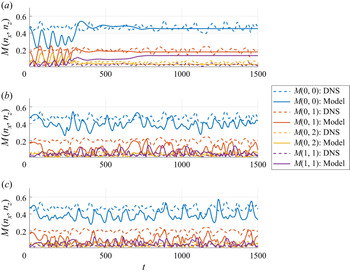
 $\boldsymbol {n}=[1,4,4]$. Figure 3 shows the time trace of the Fourier-mode energy,
 $M(n_x,n_z)$, for the three cases. In all cases, the initial condition for
 $\boldsymbol {a}$ is obtained by projecting a DNS field onto the corresponding POD mode subspace. For the six mode case, the state vector,
 $\boldsymbol {a}$, reaches a non-trivial equilibrium state after an oscillatory transient, consistent with the result of Smith et al. (Reference Smith, Moehlis and Holmes2005) (figure 3a). Given that the six mode model exhibits a stable non-trivial equilibrium (i.e.
 $\boldsymbol {a}\ne \boldsymbol {0}$), this would not be a good reference case to build a low-dimensional model exhibiting chaotic dynamics. Considering a larger number of plane Fourier modes (i.e. 25 and 41 modes), the state vector,
 $\boldsymbol {a}$, of the reduced-order model exhibits a chaotic trajectory (figure 3b,c). However, the values of
 $M(n_x,n_z)$ appear to be far off from those in DNS. In particular, the second most energetic mode of the POD-Galerkin model,
 $M(0,1)$, which would represent the time evolution of streaks, significantly deviates from DNS. Despite this issue, the presence of the chaotic dynamics in the POD-Galerkin models with 25 and 41 modes indicates that they would be good reference cases with which the other modelling approaches in § 3 can further be employed. Therefore, the remaining part of the present study will only consider the 25 and 41 mode cases.
Time trace of  $M(n_x,n_z)$ of the POD-Galerkin model: (a) six modes (Smith et al. Reference Smith, Moehlis and Holmes2005); (b) 25 modes; (c) 41 modes.

4.2. Sparse POD-Galerkin regression: POD-SINDy model
Based on the 25 and 41 mode cases in § 4.1, the optimisation problem in (3.6) is solved for  $t \in [-10\,000,0]$ with an sampling interval of
 $\Delta t = 0.5$, in order to obtain the corresponding POD-SINDy model. The model constructed is subsequently examined by considering an additional time interval
 $t \in [0, 5000]$. The relative error of the least-squares regression defined in (3.6) is reported in table 3 for the 25 mode model. Here, the relative error is defined as
 \begin{equation} \mathcal{E}_{PS} =\frac{1}{N_{{mode}}}\sum_{n_x={-}M_x}^{M_x}\sum_{n_z={-}M_z}^{M_z}\sum_{n=1}^{N_p} \frac{\left\|\left[\dot{\boldsymbol{X}}-\varTheta(\boldsymbol{X})\boldsymbol{\varXi}\right]_{n_x,n_z}^{(n)} \right\|_2}{ \left\|\left[\dot{\boldsymbol{X}}\right]_{n_x,n_z}^{(n)}\right\|_2 }, \end{equation}
where  $[\cdot ]_{n_x,n_z}^{(n)}$ indicates the component defined by the POD mode indices given in (2.4a). Here
 $N_{{mode}}$ is defined as the number of POD modes used in the sparse regression. We note that the relative error is normalised by
 $N_{mode}$ such that
 $\mathcal {E}_{PS} \in [0, 1]$. As expected, the relative error reaches the minimum when
 $\gamma$ is zero (least-squares regression). When
 $\gamma$ is increased, the relative error becomes larger due to the increased sparsification penalty as defined in (3.6).
Relative error of the least-squares regression in (3.6) for the POD-SINDy model with 25 modes. Here,  ${\mathcal {E}}_{PS}$ is defined in (4.1), which is the summation of the relative error of each mode when compared with DNS data, normalised by the total number of POD modes. The ‘training’ and ‘validation’ in second and third lines imply
 ${\mathcal {E}}_{PS}$ from
 $t\in [-10\,000,0]$ and
 $t\in [0,5000]$, respectively. Also,
 $N_0(\cdot )$ indicates the number of zero terms in the linear operator
 $\boldsymbol {L}$ and in the nonlinear operator
 $\boldsymbol {N}$, except the Reynolds shear-stress term in the mean equation, in the model. Note that the number of the POD modes used for the 25 mode POD-SINDy model is
 $N_{{mode}}=49$ due to the conjugate symmetry (i.e. one mode for the mean equation and
 $2\times 24$ modes for the fluctuation equations.

The six mode POD-SINDy model and the 25 mode POD-SINDy model obtained in this way is subsequently simulated. It is found that the POD-SINDy model rapidly blows up for  $t \in [0,4]$, and this behaviour remains unchanged for relatively low values of
 $\gamma \in [0, 0.1]$. For
 $\gamma = 1$, only
 $M(0,2)$ blows up while the rest remains relatively stable, although all the linear terms are zero in this case (see table 3). For
 $\gamma = 10$, all the terms in the regression from the Galerkin projection-template are zero, except for the nonlinear terms for the equation for
 $\dot {a}^{(1)}_{0,0}$. The application of this approach to the 41 mode case also exhibits a similar behaviour, thus it is not pursued anymore. The blow-up of the POD-SINDy model was not reported in previous studies (e.g. Brunton et al. Reference Brunton, Proctor and Kutz2016; Loiseau & Brunton Reference Loiseau and Brunton2018; Rubini, Lasagna & Da Ronch Reference Rubini, Lasagna and Da Ronch2021). However, it is worth mentioning that the dimension of nonlinear oscillations in such cases is low (e.g. Lorenz chaos, two-dimensional laminar vortex shedding, and two-dimensional cavity flows). As such, the number of POD modes considered in those studies appears to be large enough to cover the full nonlinear dynamics using sparse regression. This suggests that the blow-up of the POD-SINDy model shown here is presumably caused by the number of POD modes that are not large enough to cover the full chaotic dynamics of interest. As discussed in § 3.2, in this case, the POD-SINDy model takes the residual term
 $\boldsymbol {T}$ in the form of (3.7), which does not necessarily ensure (3.11).
4.3. Utilisation of an empirical eddy viscosity: POD-Galerkin-E model
The POD-Galerkin-E model, which utilises the simple spectral eddy viscosity of Smith et al. (Reference Smith, Moehlis and Holmes2005), is examined by considering a few values of  $\nu _t$ defined in (3.12):
 $\nu _t = (0.001,0.003,0.005)$. It is, however, found that the introduction of such a simple eddy viscosity closure does not significantly improve the accuracy of the reduced-order model compared with the original POD-Galerkin model. Indeed,
 $\nu _t=0.001$ is found to be too small to influence the original POD-Galerkin model, while
 $\nu _t=0.005$ is too large and stabilises the chaotic dynamics into a stable non-trivial equilibrium. Here, we present the results for
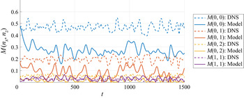
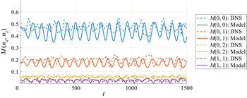
 $\nu _t=0.003$, which was determined by accounting for this observation as in Smith et al. (Reference Smith, Moehlis and Holmes2005). Figure 4 compares the time trace of
 $M(n_x,n_z)$ from DNS with that from the POD-Galerkin-E model with 25 modes for
 $\nu _t=0.003$. The mean component,
 $M(0,0)$, which contains the largest perturbation energy, exhibits a large difference from that of DNS. In fact, this deviation is greater than that of the POD-Galerkin model which does not employ any model of
 $\boldsymbol {T}$ (compare figure 4 with figure 3b). However, it should be mentioned that not all of the mode amplitudes exhibit such a deterioration. The POD-Galerkin-E model is also found to exhibit a much more improved
 $M(1,1)$ (compare figure 4 with figure 3b), indicating that the utilisation of a suitable eddy-viscosity closure would improve the performance of a reduced-order model. This will be seen in § 4.5.
Time trace of  $M(n_x,n_z)$ from DNS and the POD-Galerkin-E model with 25 modes (
 $\nu _t = 0.003$).

4.4. Sparse optimal closure: POD-Galerkin-R model
We now consider the POD-Galerkin-R model where a flexible form of eddy viscosity is determined by solving the least-squares regression problem in (3.16). The regression is performed with the data taken for  $t \in [-10\,000,0]$ with an sampling interval of
 $\Delta t = 0.5$, and the model is subsequently examined by considering an additional time interval
 $t \in [0, 5000]$. Similarly to (4.2), the relative error of the regression is defined as
 \begin{equation} \mathcal{E}_{PGR} =\frac{1}{N_{{mode}} - 1} \sum_{n_x={-}M_x}^{M_x}\sum_{n_z={-}M_z}^{M_z}\sum_{n=1}^{N_p} \frac{\|[\boldsymbol{Y}-\varTheta_e(\boldsymbol{Y}) \,{\rm diag}[\boldsymbol{c}]]_{n_x,n_z}^{(n)}\|_2}{ \|[\boldsymbol{Y}]_{n_x,n_z}^{(n)}\|_2} \end{equation}
for  $(n_x, n_z) \neq (0,0)$, and it is reported in table 4 for the 25 mode model. Note that the mode with
 $(n_x, n_z)= (0, 0)$ is excluded from the relative error statistics as no residual term was applied to this mode. As expected, the relative error becomes larger as the
 $\ell _1$-regularisation penalty,
 $\gamma _e$, increases. For
 $\gamma _e>0.005$,
 $\mathcal {E}_{PGR}$ remains unchanged, indicating that the regression would not make any improvement. In the present study, we have chosen to present the result for
 $\gamma _e=0.0005$ which renders the proposed regression sufficiently effective, while not allowing for too small values in
 $\boldsymbol {c}$ that could well be from some numerical issues (e.g. sampling time interval). We also ensure that our residual model does not overfit our training dataset by comparing the training and validation set error quantitatively as seen in table 4.
Relative error of the least-squares regression in (3.16) for the POD-Galerkin-R model with 25 modes. Here,  ${\mathcal {E}_{PGR}}$ is defined in (4.2). The ‘training’ and ‘validation’ in second and third lines imply
 ${\mathcal {E}}_{PS}$ from
 $t\in [-10\,000,0]$ and
 $t\in [0,5000]$, respectively. As in table 3,
 $N_0$ indicates the number of zero valued eddy-viscosity terms for
 $N_{{mode}}=49$.

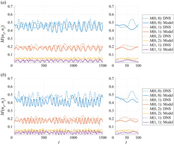
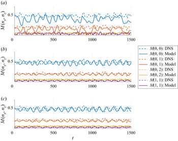
Figure 5 shows the time trace of  $M(n_x,n_z)$ from the POD-Galerkin-R model utilising 25 and 41 modes, and it is compared with that from DNS. The time traces of
 $M(n_x,n_z)$ from the POD-Galerkin-R model are now quite close to those from DNS, including the initial time evolution of the three most energetic modes (
 $M(0,0$),
 $M(0,1)$ and
 $M(0,2)$ for
 $t<50$) – note that the Lyapunov time would be expected to be of the order of the smallest time scale of the flow (i.e. the Kolmogorov time scale), which is given by
 $t\sim O(10)$ in the present case (e.g. Ruelle Reference Ruelle1979; Crisanti et al. Reference Crisanti, Jensen, Paladin and Vulpiani1993). This indicates that the performance of this model is evidently far superior to that of the POD-Galerkin and the POD-Galerkin-E models. Both of the 25 and 41 mode cases of the POD-Galerkin-R model also exhibit a chaotic oscillation with the time scale close to that of DNS, which will be discussed in § 4.5.
Time trace of  $M(n_x,n_z)$ from DNS and the POD-Galerkin-R model: (a) 25 modes (
 $\gamma _e = 0.0005$); (b) 41 modes (
 $\gamma _e = 0.0001$). The misalignment of the initial condition at
 $t = 0$ for
 $M(1,1)$ between the model and DNS data are due to the residual flow field not being capture by the POD basis.

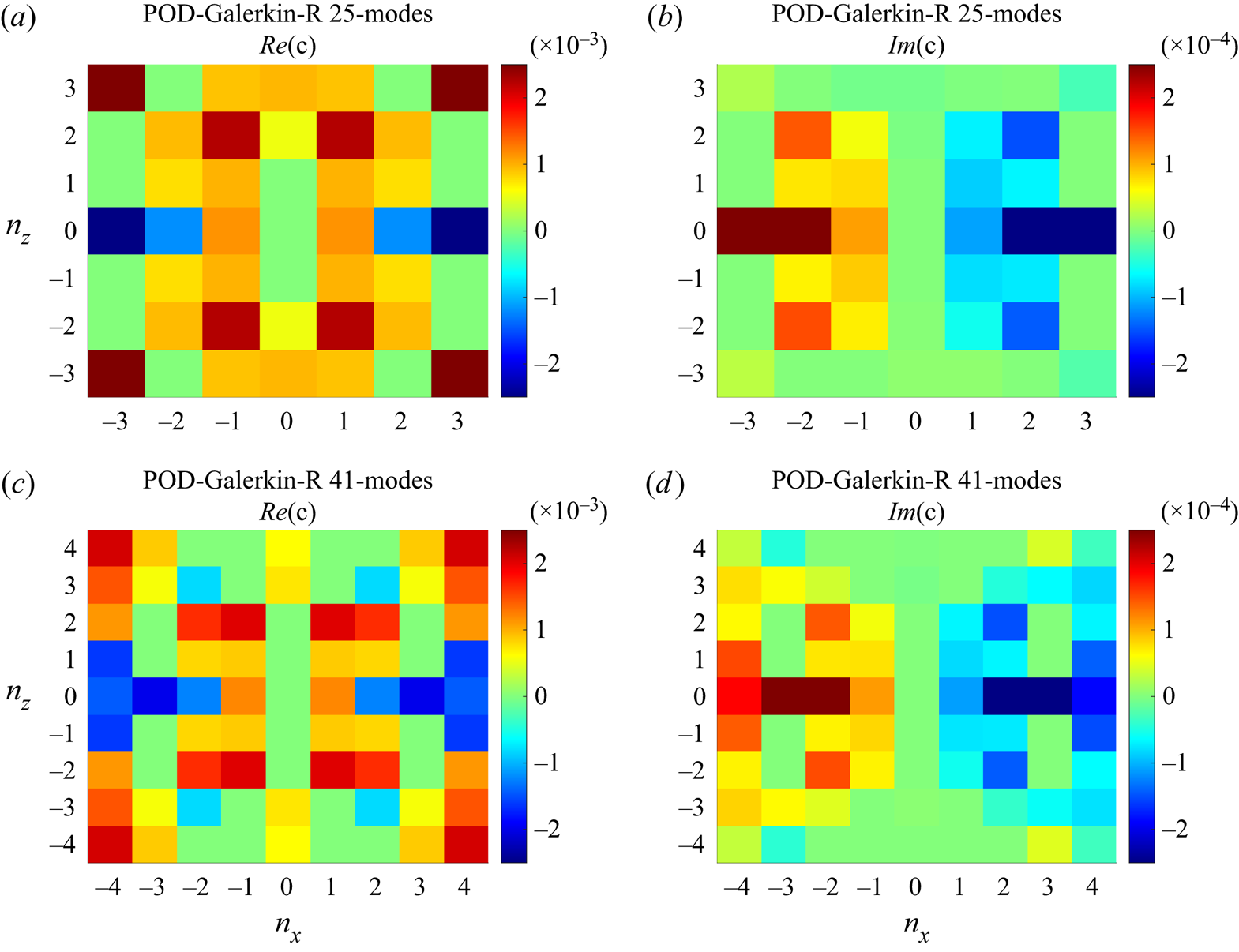
The constant vector  $\boldsymbol {c}({=}c^{(n)}_{n_x,n_z})$ used for the eddy viscosity in (3.13b) is also visualised in figure 6. We first consider the 25 mode case (figure 6a). Here, we note that the constant vector,
 $\boldsymbol {c}$, exhibits a conjugate symmetry because the velocity in this study is real valued. It also appears to be distributed highly symmetrically in the
 $n_x$–
 $n_z$ plane. This originates from the
 $\mathcal {R}$ symmetry in (2.6) – the
 $\mathcal {R}$ symmetry imposes that the streamwise and wall-normal components of
 $\boldsymbol {\phi }_{n_x,n_z}^{(n)}$ and
 $\boldsymbol {\phi }_{n_x,-n_z}^{(n)}$ are to be identical, and their spanwise component to have opposite signs, while the energy of the streamwise component dominates over the other two components (see also figure 7). The real part of
 $\boldsymbol {c}$, proportional to the strength of dissipation (i.e. the removal of the energy from the given dynamics), is positive for most pairs of
 $(n_x,n_z)$ in the
 $n_x\text{--} n_z$ plane, as expected from (3.11). However, there are some
 $c^{(n)}_{n_x,n_z}$ which exhibit negative values, and this is particularly pronounced around
 $(n_x,n_z)=(\pm 3,0)$. This indicates that allowing for negative elements of
 $\boldsymbol {c}$ does help to improve the performance of the reduced-order model as discussed in § 3.4. It is interesting to note that the higher streamwise and spanwise independent modes are energised (inverse energy transfer) and dissipated (forward energy cascade), respectively, consistent with the findings from Podvin (Reference Podvin2009). Furthermore, some
 $c^{(n)}_{n_x,n_z}$ also exhibit non-zero imaginary values. However, their amplitudes are overall an order-of-magnitude smaller than those of the real counterpart, implying that the dispersive effect imposed by the imaginary part of
 $c^{(n)}_{n_x,n_z}$ would not be significant. Finally, the distribution of
 $c^{(n)}_{n_x,n_z}$ for the 41 mode case (figure 6c,d) shows that increasing the number of POD modes do not significantly change the overall distribution and strength of
 $c^{(n)}_{n_x,n_z}$ in the
 $n_x$–
 $n_z$ plane (compare figure 6a,b with figure 6c,d). We note that as the number of POD modes is increased, the eddy viscosity also needs to vanish. However, this is not observed in figure 6. Instead, the similar distribution of
 $c^{(n)}_{n_x,n_z}$ for the 25 and 41 mode cases suggests that the eddy viscosity obtained with (3.16) is coherently compensating for some physical processes which are not simply resolved by the increase in the number of plane Fourier modes (i.e.
 $M_x$ and
 $M_z$). In this respect, it is worth remembering that the reduced-order models in the present study only considers the leading POD mode for each
 $(n_x,n_z)$. One can therefore presume that the compensation made by the eddy viscosity model is associated with the lack of the higher-order POD modes for each
 $(n_x,n_z)$.
Distribution of real (a,c) and imaginary (b,d) part of  $c^{(n)}_{n_x,n_z}$ in the
 $n_x \text{--} n_z$ plane: (a,b) 25 modes (
 $\gamma _e = 0.0005$); (c,d) 41 modes (
 $\gamma _e = 0.0001$).

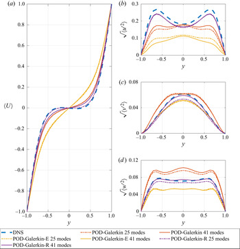
Turbulence statistics from DNS and the reduced-order models: (a) streamwise mean velocity; (b–d) root-mean-squared velocity fluctuations.

4.5. Comparison of the reduced-order models
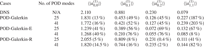
Having examined all of the reduced-order models introduced in § 3, their performance is compared in this subsection. Table 5 shows the time-averaged amplitudes of the four leading POD modes from DNS and the reduced-order models, except the POD-SINDy model whose solution was found to blow up (see § 4.2). We note that the four POD modes contain approximately 95 % of total perturbation kinetic energy (see table 1). The POD-Galerkin model performs sensibly only for the mean component,  $a^{(1)}_{0,0}$, while the rest of the components with
 $(n_x,n_z) \neq (0,0)$ exhibit considerable errors ranging from 50 % to 200 %. The addition of an empirical eddy viscosity does not improve the POD-Galerkin model greatly (i.e. POD-Galerkin-E model), since the model still shows errors of 50 %–80 % across all the four leading POD modes. This model may also be viewed to perform most poorly, given the largest errors for
 $a^{(1)}_{0,0}$ that contain the largest amount of perturbation energy. Finally, the POD-Galerkin-R model shows the best performance and it has only a maximum 16 % error for the first three leading POD modes. Although this model still shows a relatively large error for
 $a^{(1)}_{1,1}$, the energy contained by this mode in DNS is only approximately 1 % (see table 1). Therefore, this error would be relatively insignificant.
Time-averaged amplitudes of POD modes from DNS and the reduced-order models. Here, the numbers in the parenthesis indicate the relative error to the values from DNS.

The mean and turbulent velocity fluctuations from DNS and the reduced-order models are compared in figure 7. As expected from table 5, the mean velocity from the POD-Galerkin model and the POD-Galerkin-R model shows the best agreement with that from DNS. However, the POD-Galerkin model exhibits large differences in the velocity fluctuation profiles, while the statistics from the POD-Galerkin-E model are overall damped. A closer inspection reveals that the cross-stream and wall-normal turbulence fluctuations are predicted better by the 41 mode model, with a slightly poorer prediction in the streamwise mean velocity as compared with the 25 mode model. In any case, the level of agreement of the POD-Galerkin-R models in turbulence statistics has not been observed in any of the previous reduced-order models in PCF (e.g. Smith et al. Reference Smith, Moehlis and Holmes2005; Cavalieri Reference Cavalieri2021).
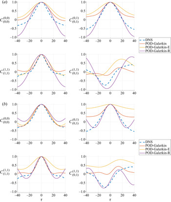
Next, to assess the dynamical behaviour of the leading POD modes from the reduced-order models, the following temporal autocorrelation and cross-correlation of the main observables defined in (2.2) are computed:
 \begin{equation} C^{(n_x,n_z)}_{(m_x,m_z)}(\tau) = \frac{\langle \tilde{M}(t + \tau ; n_x,n_z) \tilde{M}(t ; m_x,m_z) \rangle}{\sqrt{\tilde{M}^{2}(t; n_x,n_z)}\sqrt{\tilde{M}^{2}(t; m_x,m_z)}}, \end{equation}
where  $\tilde {M}(t;n_x,n_z) = M(t;n_x,n_z) - \langle M(t;n_x,n_z)\rangle$. Figure 8 compares the correlation functions of the 25 mode and 41 mode models considered with those of DNS. In general, for the temporal correlations of
 $C^{(0,1)}_{(0,1)}$, the POD-Galerkin-R model have a closer match with the DNS data when compared with POD-Galerkin and POD-Galerkin-E models. The inclusion of more POD modes have the effect of improving the correlations of
 $C^{(1,1)}_{(1,1)}$ especially for
 $\tau = [-15,15]$. By doing so, we observe a notable improvement of the
 $C^{(1,1)}_{(0,1)}$ correlations, an important behaviour expected from the SSP, as it captures the breakdown of a streak structure and the regeneration of the streamwise vortices. Neither the POD-Galerkin or the POD-Galerkin-E model were able to closely replicate this behaviour with the inclusion of more POD modes.
Temporal autocorrelation and cross-correlation of (a) 25 modes ( $\gamma _e = 0.0005$ for the POD-Galerkin-R model); (b) 41 modes (
 $\gamma _e = 0.0001$ for the POD-Galerkin-R model).

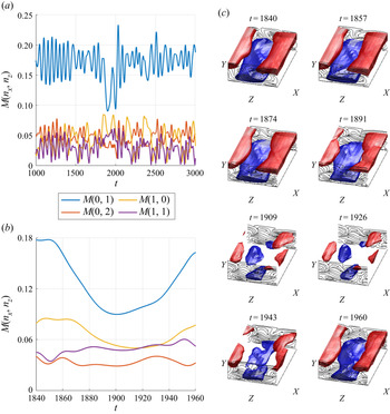
Finally, figure 9 shows a time trace of the observables defined in (2.2) and a set of flow field snapshots visualising a SSP generated by the POD-Galerkin-R 41 mode model. The strong streaky motions are apparent in  $t=1840\text{--} 1857$, shown as a peak in
 $M(0,1)$ in figure 9(b). The streaks break down into a wavy behaviour from
 $t=1874\text{--} 1891$, accompanied by a decrease in
 $M(0,1)$ and an increase in
 $M(1,0)$ in figure 9(b). The streaks break down completely from
 $t=1909\text{--} 1926$ while the quasi-streamwise vortices are regenerated, leading to an increase in
 $M(1,1)$. Finally, the quasi-streamwise vortices feed energy to the streaks from
 $t=1943 \text{--} 1960$, known as the ‘lift-up’ effect. We note that the SSP from the POD-Galerkin-R 41 mode model is qualitatively similar to that of figure 1, supporting the good agreements in temporal autocorrelation and cross-correlation of figure 8.
Time trace of  $M(0,1)$,
 $M(0,2)$,
 $M(1,0)$,
 $M(1,1)$ obtained from the POD-Galerkin-R 41 mode model (a) for
 $t=1000\text{--} 3000$ and (b) for
 $t=1840\text{--} 1960$. (c) Flow snapshots at
 $t=1840, 1857, 1874, 1891, 1909, 1926, 1943, 1960$, where the blue and red isosurfaces indicate
 $u=\pm 0.38$, respectively.

5. Concluding remarks
In the present study, we have examined a set of physics-informed and data-driven approaches towards the development of a low-dimensional model which is more accurate than the conventional ones for turbulent wall-bounded shear flows. Based on the utilisation of POD modes, a particular focus is given to the case where the number of the POD modes is not necessarily large enough to cover the full dynamics of the given chaotic state. Starting from the conventional POD-Galerkin model, three additional approaches have been examined: (1) sparse regression of the POD-Galerkin dynamics (POD-SINDy model); (2) POD-Galerkin projection with an empirical eddy viscosity model (POD-Galerkin-E model; Smith et al. (Reference Smith, Moehlis and Holmes2005)); (3) a newly proposed POD-Galerkin projection with an optimal eddy viscosity determined using a spare regression (POD-Galerkin-R model). The sparse regression of the POD-Galerkin dynamics has been found to be unsuccessful presumably due to the small number of POD modes considered, although this might be able to be improved by incorporating the energy-preserving nonlinearity constraint into the model (Loiseau & Brunton Reference Loiseau and Brunton2018). In the present study, this issue can be tackled by introducing a data-driven eddy-viscosity model for a highly turbulent flow, as the POD-Galerkin projection with a sparse optimal viscosity has been found to well approximate the given chaotic dynamics. It should be mentioned that this eddy-viscosity model was introduced to have a better nonlinear energy balance (3.8) only at large scale spanned by the POD modes of interest (see also discussion in § 3.3). In this respect, the data-driven eddy-viscosity model here may be viewed to be a pragmatic alternative to the energy-preserving nonlinearity constraint in Loiseau & Brunton (Reference Loiseau and Brunton2018) for highly turbulent flows.
The key reason for the success of the POD-Galerkin-R model is that it considers the largest amount of physical information: i.e. Galerkin projection and energy cascade. It is important to emphasise that the Galerkin projection allows the reduced-order model to inherit the mathematical structure of the Navier–Stokes equations. In other words, this feature makes the reduced-order model analysable, as it contains all the mathematical elements previously utilised to study the flow physics: e.g. linearised dynamics and production/dissipation, etc. Having said this, the energy cascade via nonlinear and non-local interactions modelled here is still an active and challenging research topic (e.g. Vassilicos Reference Vassilicos2015), and it may take years to gain a full physical understanding, if it is not impossible. The eddy-viscosity model utilised in the present study is still very minimal to incorporate the full energy cascade dynamics into a reduced-order model. However, a notable point of doing so is that a data-driven approach (i.e. sparse regression), which itself does not provide any insight into the given flow physics, was applied to model the flow physics which is not fully understood. We have shown that classical physics-based reduced-order modelling (i.e. POD-Galerkin) of a complex process is limited, and data-driven approaches can be exploited to improve the reduced-order models.
It should also be mentioned that there have recently been a surge of data-driven flow modelling approaches using optimisation and machine learning (see the recent review by Brunton, Noack & Koumoutsakos (Reference Brunton, Noack and Koumoutsakos2020)). In the context of reduced-order modelling, utilisation of some machine learning algorithms (e.g. reservoir computing) was proposed for the prediction of a chaotic dynamical system (e.g. Pathak et al. (Reference Pathak, Hunt, Girvan, Lu and Ott2018) and the other recent studies). While such an approach may well be practically useful for the prediction of extreme events relevant to weather forecasting, it does not offer insights into the flow physics required for modelling in a wider context. Indeed, how one would smartly incorporate the known flow physics into a data-driven modelling approach has been a central issue of many current investigations, especially when the equations of motion (e.g. Navier–Stokes equations) are fully available. In this respect, the utilisation of Galerkin projection in the present study may perhaps provide a new opportunity as it directly offers a mathematical structure from the governing equations. Indeed, instead of utilising a model given by (3.13), a highly flexible form of model for  $\boldsymbol {T}$ may well be considered with a machine learning algorithm.
It is also worth mentioning about the extrapolation capability of the model obtained at a given set of parameters to the others. This issue has often been regarded to be generally challenging for a model reduction problem. In the present study, the optimal eddy viscosity obtained here is, in fact, intricately linked to the physical processes of the given system. The optimal value would vary with the change of system parameters (e.g. the Reynolds-number-dependent role of small scales modelled with the eddy viscosity here). Therefore, further efforts need to be made to address this issue in the future.
Finally, given the original scope of the present paper discussed in § 1.1, the natural next step of the present study is to apply the approach proposed here to flows at higher Reynolds numbers where coherent structures begin to emerge at multiple integral length scales as in the attached eddy hypothesis of Townsend (Reference Townsend1956, Reference Townsend1976). An obvious issue for this next step would lie in the determination of the number of POD modes that capture the core interaction dynamics at integral length scales, while effectively excluding the dissipative dynamics that can be modelled using the data-driven eddy-viscosity approach here. Once this process is completed with an appropriate validation using DNS data, invariant solutions (e.g. unstable periodic orbits) of the reduced-order model can subsequently be computed to study the multiscale dynamics. The current hope is that the total degree of freedom of the reduced-order model remains at  $O(10^{2}\text{--} 10^{3})$ at a sufficiently high Reynolds number (e.g.
 $Re_\tau \simeq 500\text{--} 1000$) to tackle this challenge.
Funding
Y.H. gratefully acknowledges the financial support of the Leverhulme Trust (RPG-2019-123) and the Engineering and Physical Sciences Research Council (EPSRC; EP/T009365/1) in the UK.
Declaration of interests
The authors report no conflict of interest.
Appendix A. Galerkin projection
The projection of (2.4a) onto the Navier–Stokes equations (2.1) leads to the following system of ordinary differential equations:
 \begin{equation} \dot{a}_{n_x,n_z}^{(n)} = \sum_{m=1}^{N_p}{L}^{(n,m)}_{n_x,n_z} {a}_{n_x,n_z}^{(m)} +{\mathcal{N}}_{n_x,n_z}^{(n)}, \end{equation}
where
 \begin{equation} \mathcal{N}_{n_x,n_z}^{(n)}= \sum_{k_x={-}N_x}^{N_x} \sum_{k_z={-}N_z}^{N_z} \sum_{k=1}^{N_p} \sum_{m=1}^{N_p} {N}_{\substack{n_x,n_z \\ k_x,k_z}}^{(n,k,m)} \ a^{(k)}_{k_x,k_z} a^{(m)}_{\substack{ m_x = n_x - k_x \\ m_z = n_z - k_z}}, \end{equation}
with
 \begin{align} {L}^{(n,m)}_{n_x,n_z} &={-} \frac{1}{Re}\left[ \left(\dfrac{2{\rm \pi} n_x}{L_x}\right)^{2} + \left(\dfrac{2{\rm \pi} n_z}{L_z}\right)^{2} \right] \delta_{nm} - \frac{1}{Re} \int_y \left(\frac{\mathrm{d}{\boldsymbol{\phi}}^{(m)}_{n_x,n_z}}{\mathrm{d} y}\right)^{H} \frac{\mathrm{d}{\boldsymbol{\phi}}^{(n)}_{n_x,n_z}}{\mathrm{d} y} \,\mathrm{d} y\nonumber\\ &\quad - \left( \frac{2{\rm \pi} {\rm i} n_x}{L_x} \right) \int_y y (\boldsymbol{\phi}^{(m)}_{n_x,n_z})^{H} \boldsymbol{\phi}^{(n)}_{n_x,n_z} \, \mathrm{d} y - \int_y (\phi^{(m)}_{2,n_x,n_z})^{H} {\phi}^{(n)}_{1,n_x,n_z} \, \mathrm{d} y \end{align}
and
 \begin{align} {N}_{\substack{n_x,n_z \\ k_x,k_z}}^{(n,k,m)} ={-}\dfrac{1}{\sqrt{L_x L_z}} \int_y (\boldsymbol{\phi}^{(n)}_{n_x,n_z})^{H} \begin{bmatrix} \dfrac{2 {\rm \pi}{\rm i} k_x}{L_x} {\boldsymbol{\phi}}^{(k)}_{k_x,k_z} \dfrac{\mathrm{d}{\boldsymbol{\phi}}^{(k)}_{k_x,k_z}}{\mathrm{d} y} \dfrac{2 {\rm \pi}{\rm i} k_z}{L_z} {\boldsymbol{\phi}}^{(k)}_{k_x,k_z} \end{bmatrix} {\boldsymbol{\phi}}^{(m)}_{\substack{m_x = n_x - k_x\\m_z = n_z - k_z}} \, \mathrm{d} y. \end{align}
Therefore, (A1) may be written as the following quadratic nonlinear dynamical system form:
 \begin{equation} \dot{\boldsymbol{a}}=\boldsymbol{La}+\boldsymbol{N}(\boldsymbol{a},\boldsymbol{a}), \end{equation}
where  $\boldsymbol {a}$ is defined as a column vector, each element of which is given by
 $a_{n_x,n_z}^{(n)}$,
 \begin{equation} \boldsymbol{La}\equiv \sum_{m=1}^{N_p}{L}^{(n,m)}_{n_x,n_z} {a}_{n_x,n_z}^{(m)} \end{equation}
and
 \begin{equation} \boldsymbol{N}(\boldsymbol{a},\boldsymbol{a}) \equiv {\mathcal{N}}_{n_x,n_z}^{(n)}. \end{equation}
Similarly, the diffusion operator used for the eddy-viscosity closure in §§ 3.3 and 3.4 is defined as
 \begin{equation} \boldsymbol{Da}\equiv \sum_{m=1}^{N_p}{D}^{(n,m)}_{n_x,n_z} {a}_{n_x,n_z}^{(m)}, \end{equation}
where
 \begin{equation} {D}^{(n,m)}_{n_x,n_z} ={-} \left[ \left(\dfrac{2{\rm \pi} n_x}{L_x}\right)^{2} + \left(\dfrac{2{\rm \pi} n_z}{L_z}\right)^{2} \right] \delta_{nm} - \int_y \left(\frac{{\rm d}{\boldsymbol{\phi}}^{(n)}_{n_x,n_z}}{{\rm d} y}\right)^{H} \frac{{\rm d}{\boldsymbol{\phi}}^{(m)}_{n_x,n_z}}{{\rm d} y} \, {{\rm d} y} \end{equation}
for  $(n_x,n_z) \neq (0,0)$ and
 \begin{equation} {D}^{(n,m)}_{n_x,n_z} = 0 \end{equation}
for  $(n_x,n_z) = (0,0)$, so that the eddy viscosity is not applied to the mean equation. Using the diffusion operator above, the eddy-viscosity model defined in (3.13) is finally written as
 \begin{equation} \boldsymbol{V}_t\boldsymbol{Da}\equiv c_{n_x,n_z}^{(n)} e(t)\sum_{m=1}^{N_p}{D}^{(n,m)}_{n_x,n_z} {a}_{n_x,n_z}^{(m)}, \end{equation}
where  $c_{n_x,n_z}^{(n)}$ forms each element of
 $\boldsymbol {c}$ in (3.13).
Appendix B. The choice of  $e$ in § 3.4

Here, we report a POD-Galerkin-R model, in which  $e(t)=\boldsymbol {a}^{H}\boldsymbol {a}$ is considered instead of
 $e(t)=a_{0,0}^{(1)}$. The sparse regression in (3.16) is performed with the DNS data for
 $t\in [-10\,000,0]$ and the resulting model is subsequently examined for
 $t\in [0,5000]$. The time trace of
 $M(n_x,n_z)$ from the reduced-order model and from DNS is shown in figure 10. Overall, the mean of
 $M(n_x,n_z)$ and its oscillation time scale from the reduced-order model compare fairly well with those from DNS. The oscillation magnitude of
 $M(0,0)$ in this case is slightly stronger than that from the POD-Galerkin-R model with
 $e(t)=a_{0,0}^{(1)}$ (figure 5a), and the oscillation appears to be slightly less chaotic.
Time trace of  $M(n_x,n_z)$ from DNS and the POD-Galerkin-R model (
 $\gamma _e = 0.0005$ and
 $e(t)=\boldsymbol {a}^{H}\boldsymbol {a}$) with 25 modes.

Appendix C. The effect of $\gamma _e$ on model dynamics

The sparsity-promoting  ${\ell }_1$-regulariser acts as a control parameter balancing between the effect of the Galerkin projection model and the residual model on the overall dynamics. In figure 11, we observe that for
 $\gamma _e = 0.001$, the effect of the residual model adversely affects the temporal dynamics as only certain POD modes are being selectively damped. For
 $\gamma _e = 0.0003$, the residual model dominates and the POD modes are strongly coupled to the mean POD mode where we obtain oscillatory behaviour due to excessive damping.
Time trace of  $M(n_x,n_z)$ from DNS and the POD-Galerkin-R of the 25 mode model: (a)
 $\gamma _e = 0.001$; (b)
 $\gamma _e = 0.0005$; (c)
 $\gamma _e = 0.0003$.