1. Introduction
Charging processes of plasma-embedded objects or dust grains are one of the most important problems in plasma physics. Applications range from space physics to plasma probe theory (Shukla & Mamun Reference Shukla and Mamun2002). Dust grains become charged because plasma particles hit the grain surface and will be absorbed. Due to the larger mobility of electrons, and in the absence of other processes, grains acquire typically a negative floating charge. Subsequently, the resulting electric field repels electrons and attracts ions. A dynamical equilibrium charge or potential is reached when the electron and ion currents to the grain are equal. The orbital motion limited (OML) theory of Mott-Smith & Langmuir (Reference Mott-Smith and Langmuir1926) describes an equilibrium potential as a function of the plasma parameters for an isolated dust grain in a collisionless plasma, but it is only a good approximation for thick sheaths where the grain radius is small in comparison to the plasma Debye length. For larger grains, the potential profile of the grain becomes such that the assumptions underlining the OML theory are no longer valid, and thus numerical treatment is necessary. The charging currents are substantially changed if an external magnetic field is present. Plasma particles become magnetized when their motion is aligned with the field lines, and the rotation symmetry of the charging currents no longer exists. Based on the OML approach, a qualitative analysis of how the charging currents in a magnetized plasma are affected is given in Tsytovich, Sato & Morfill (Reference Tsytovich, Sato and Morfill2003). They argue that a situation of magnetized electron but unmagnetized ion charging current can exist, since the electron gyration radius is always smaller than that of ions and therefore its motion is more strongly coupled to the magnetic field than the ions.
In this work the charging of single, stationary and spherical dust grains of different radii in self-consistent, fully 3-D PIC simulations are studied. A plasma consisting of ions and electrons is considered with and without an overlapping, constant magnetic field. The resulting equilibrium potential is compared to the current state of the literature.
2. Theory of dust grain charging and equilibrium surface potential
The OML theory considers collisionless ion and electron trajectories in a central potential and allows the determination of the collection cross-sections from conservation laws of energy and angular momentum. The integral of the corresponding cross-section and the Maxwellian velocity distribution gives the ion and electron currents to an isolated grain of radius
 $R$
(Mott-Smith & Langmuir Reference Mott-Smith and Langmuir1926):
 $$\begin{eqnarray}\displaystyle & \displaystyle I_{i}^{OML}=4{\rm\pi}R^{2}e^{}n_{0}\sqrt{\frac{kT_{i}}{2{\rm\pi}m_{i}}}\left(1-\frac{e^{}V_{R}}{kT_{i}}\right) & \displaystyle\end{eqnarray}$$
 $$\begin{eqnarray}\displaystyle & \displaystyle I_{e}^{OML}=4{\rm\pi}R^{2}e^{}n_{0}\sqrt{\frac{kT_{e}}{2{\rm\pi}m_{e}}}\exp \left(\frac{e^{}V_{R}}{kT_{e}}\right), & \displaystyle\end{eqnarray}$$
 $T_{i}$
,
 $T_{e}$
and
 $m_{i}$
,
 $m_{e}$
are the ion/electron temperature and mass, respectively.
 $n_{0}=n_{i}=n_{e}$
is the ion/electron number density,
 $V_{R}$
is the grain surface potential,
 $k$
is the Boltzmann constant and
 $e^{}$
the elementary charge. The equilibrium surface potential follows from equating ion and electron current (
 $I_{i}^{OML}=I_{e}^{OML}$
) to the charging equation:
 $$\begin{eqnarray}\sqrt{\frac{m_{i}}{m_{e}}}\frac{1}{\sqrt{{\it\beta}}}=\left(1-\frac{{\it\eta}_{R}}{{\it\beta}}\right)\exp (-{\it\eta}_{R}),\end{eqnarray}$$
where
 ${\it\eta}_{R}=e^{}V_{R}/kT_{e}$
is the normalized surface potential and
 ${\it\beta}=T_{i}/T_{e}$
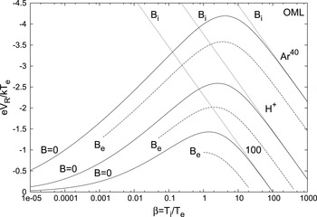
the ratio of ion-to-electron temperature. Figure 1 shows the results for (2.3) plotted against a logarithmic scale in
 ${\it\beta}$
for mass ratio
 $m_{i}/m_{e}$
of argon
 $\text{Ar}^{40}$
(
 $73\,609$
, upper solid line), hydrogen
 $\text{H}^{+}$
(
 $1836.2$
, centre solid line) and
 $100$
(lower solid line), which are common in the literature for numerical investigations. The surface potential is independent of the grain radius
 $R$
. Larger mass ratios result in more negative surface potentials because of the lower ion energy in comparison to that of electrons. With decreasing temperature ratio
 ${\it\beta}$
the normalized surface potential
 ${\it\eta}_{R}$
asymptotically tends towards zero, since the ion energy decreases and therefore they will be accelerated nearby and radially to the grain and the number of reflected ions disappears. The absolute value of
 ${\it\eta}_{R}$
can only increase with
 ${\it\beta}$
until it is greater than
 ${\it\beta}$
. The maximum is reached if
 ${\it\eta}_{R}$
(absolute value) is equal to
 ${\it\beta}$
. Further increase of
 ${\it\beta}$
results in a decreasing negative surface potential, since the ion energy approaches that of electrons.
 ${\it\eta}_{R}$
becomes zero if the mass ratio is equal to that of the temperature
 ${\it\beta}$
, because ions and electrons are then at the same energy level and the grain cannot acquire a surface potential. The ion temperature is normally smaller or equal to that of electrons and why the case of
 ${\it\beta}>1$
is rather of academic nature. In the OML approach it is explicitly assumed that no potential barriers appear in the effective potential energy of the ions. Thus, OML theory is only an approximation for thick sheaths where the grain radius is smaller than the plasma Debye length of both ions and electrons (
 $R<{\it\lambda}_{i},{\it\lambda}_{e}$
) (Lampe Reference Lampe2001; Fortov et al.
Reference Fortov, Ivlev, Khrapak, Khrapak and Morfill2005). The more general orbital motion (OM) theory includes the potential and ion trajectory distributions around the grain, but requires numerical treatment. For thin sheaths where
 $R>{\it\lambda}_{i},{\it\lambda}_{e}$
the potential profile of the grain becomes such that potential barriers can appear for ions moving towards the grain and will be reflected from these barriers, which leads to a reduced ion charging current. Hence the equilibrium surface potential becomes more negative with increasing grain radius (Kennedy & Allen Reference Kennedy and Allen2003).
The normalized surface potential
 $e^{}V_{R}/kT_{e}$
plotted against the temperature ratio
 ${\it\beta}=T_{i}/T_{e}$
in logarithmic scale for the mass ratio
 $m_{i}/m_{e}$
of argon
 $\text{Ar}^{40}$
(
 $73\,609$
, three upper lines), hydrogen
 $\text{H}^{+}$
(
 $1836.2$
, three centre lines) and
 $100$
(three lower lines). The solid lines (
 $B=0$
) represent results from the unmodified OML approach without a magnetic field (2.3), the dashed lines (
 $B_{e}$
) are according to the case of a magnetized electron but unmagnetized ion current if
 ${\it\gamma}_{i}<1<{\it\gamma}_{e}$
(2.5) and the dotted lines (
 $B_{i}$
) represents the fully magnetized case if
 ${\it\gamma}_{i},{\it\gamma}_{e}>1$
(2.7).

If an external magnetic field is present, ion and electron trajectories are forced into circular or spiral paths. The Larmor radius or gyroradius
 $r_{g}$
(radius of gyration) follows by equating the Lorentz and centripetal forces and in a Maxwellian plasma, the most probable gyroradius
 $r_{g}^{mp}$
can be defined as follows:
 $$\begin{eqnarray}r_{g}^{mp}=\frac{mv_{mp}}{2e^{}B}=\sqrt{\frac{mkT}{2}}\frac{1}{e^{}B},\end{eqnarray}$$
where
 $v_{mp}=\sqrt{2kT/m}$
is the most probable velocity according to Maxwell and
 $B$
the strength of the magnetic field. With the factor of
 $2$
an equal distribution of the velocity magnitude parallel and perpendicularly to the magnetic field is assumed. It follows from (2.4) that the electron gyroradius is typically smaller than that of the ions, for which reason electrons are more strongly coupled to the magnetic field than the ions. In Tsytovich et al. (Reference Tsytovich, Sato and Morfill2003) it is argued that if the magnetic field becomes so large that the electron gyroradius is equal to the grain collection radius
 ${\rm\pi}R^{2}$
, the charging current lose its rotation symmetry and the electrons can be considered as moving along the field lines and straight towards the grain. Therefore, the spherical cross-section of
 $4{\rm\pi}R^{2}$
in (2.2) has to be replaced by
 $2{\rm\pi}R^{2}$
, where the factor of
 $2$
takes into account a bidirectional arrival. The electron charging current is reduced by half, while the ion current stays approximately the same if the magnetic field is not so strong that the ion gyroradius is still larger than the grain radius. For this case the charging equation follows from
 $I_{i}^{OML}=I_{e}^{OML}/2$
:
 $$\begin{eqnarray}\sqrt{\frac{m_{i}}{m_{e}}}\frac{1}{\sqrt{{\it\beta}}}=2\left(1-\frac{{\it\eta}_{R}}{{\it\beta}}\right)\exp (-{\it\eta}_{R})\quad \text{for }{\it\gamma}_{i}<1<{\it\gamma}_{e},\end{eqnarray}$$
where
 ${\it\gamma}_{i,e}=R/r_{gi,ge}^{mp}$
is the ratio of the grain radius to the most probable gyroradius for ions/electrons, respectively. The charging equation (2.5) describes the case of a magnetized electron but unmagnetized ion current and is shown in figure 1 by the dashed lines. The reduced electron current results in a decrease of the negative surface potential. Following the condition
 ${\it\gamma}_{i}<1<{\it\gamma}_{e}$
, the dashed lines are only shown for
 ${\it\gamma}_{e}/{\it\gamma}_{i}=r_{gi}^{mp}/r_{ge}^{mp}\geqslant 10$
, because the gyroradius depends on the temperature, see (2.4). The factor
 $10$
has been chosen arbitrarily. With (2.4), the condition
 ${\it\gamma}_{i}<1<{\it\gamma}_{e}$
can also be expressed by the strength of the magnetic field:
 $$\begin{eqnarray}B_{i}=\sqrt{\frac{m_{i}kT_{i}}{2}}\frac{1}{e^{}R}>B>\sqrt{\frac{m_{e}kT_{e}}{2}}\frac{1}{e^{}R}=B_{e}.\end{eqnarray}$$
Above the critical magnetic field
 $B_{e}$
, the charging process of the dust grains changes substantially. In Chang & Spariosu (Reference Chang and Spariosu1993) it is shown with numerical modelling that for
 ${\it\gamma}_{e}<1$
the effect of the magnetic field on dust particle charging can be neglected. For magnetic fields stronger than
 $B_{i}$
, the ion gyroradius becomes smaller than
 $R$
and the cross-section in (2.1) must also be replaced by
 $2{\rm\pi}R^{2}$
. In addition, the ion charging current becomes independent of the attracting surface potential, because every ion which moves along a field line penetrates the grain surface will be absorbed. For the fully magnetized case the charging equation follows from
 $I_{i}^{OML}(V_{R}=0)/2=I_{e}^{OML}/2$
:
 $$\begin{eqnarray}\sqrt{\frac{m_{i}}{m_{e}}}\frac{1}{\sqrt{{\it\beta}}}=\text{e}^{-{\it\eta}_{R}}\quad \text{for }{\it\gamma}_{i},{\it\gamma}_{e}>1,\end{eqnarray}$$
where the condition
 ${\it\gamma}_{i},{\it\gamma}_{e}>1$
is equivalent to a magnetic field strength of
 $B>B_{i}$
. The fully magnetized case is shown in figure 1 by the dotted lines. The reduced ion current leads to a more negative surface potential with decreasing ion temperature. The cases where
 $B\leqslant B_{e}$
or
 $B\approx B_{i}$
can only be treated numerically. In addition, when the results are based on a modified OML theory, the behaviour of dust grains with
 $R>{\it\lambda}_{i},{\it\lambda}_{e}$
in a magnetized plasma can also only be examined with numerical investigations.
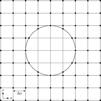
A Cartesian grid system (for simplicity two-dimensional) with a single, spherical dust grain in the centre. The radius of the sphere is an integer multiple of the grid spacing
 ${\rm\Delta}x$
(here
 $R=2\,{\rm\Delta}x$
). To reflect the spherical structure, reduced grid point distances (dashed lines) are considered in the Poisson solver. The points on the grain surface are set in every simulation time step to the surface potential
 $V_{R}$
. The grid points inside the sphere are not relevant for the simulation.

3. Simulation method
Our simulation tool is the OPAR (Open architecture PARticle in cell simulation) code, which is a fully 3-D, electrostatic particle-in-cell (PIC) code with a single, spherical dust grain in the centre of a Cartesian coordinate grid system (Lange Reference Lange2015). The integration of the sphere into the grid is illustrated in figure 2. For simplicity, only a 2-D grid system with a circle is depicted. The radius of the sphere is an integer multiple of the grid spacing
 ${\rm\Delta}x$
to reflect the spherical structure, and the reduced grid point distances (dashed lines) have been included into the Poisson solver. The points on the grain surface are set in every time step to the surface potential
 $V_{R}$
. The grid points inside the sphere are not relevant for the simulation. The surface of the sphere is treated as an inner boundary, plasma particles reaching the grain surface are removed from the simulation and their charge is accumulated to the floating surface charge
 $Q_{R}$
. The correlation between the surface charge and potential is given by the grain capacitance
 $C$
:
 $$\begin{eqnarray}V_{R}=\frac{Q_{R}}{C}.\end{eqnarray}$$
The capacitance depends on material and plasma properties, but is set here in all simulations to the vacuum value
 $C=4{\rm\pi}{\it\varepsilon}_{0}R$
. At the outer boundary of the simulation box, particles can leave the system and will be removed. New particles are injected at all boundary grid cells with a thermal velocity according to Maxwell. The number of injected particles per time step and grid cell follows from the given current density. This injection method represents an infinite plasma medium with constant density outside the simulation box. The algorithm is the same as those widely used in the literature (Birdsall & Langdon Reference Birdsall and Langdon1991). Ions and electrons are considered dynamically in a collisionless Maxwellian plasma with
 $n_{0}=n_{i}=n_{e}=6\times 10^{15}~\text{m}^{-3}$
and an electron temperature of
 $kT_{e}=1~\text{eV}$
, which corresponds to an electron Debye length of
 ${\it\lambda}_{e}=95.98~{\rm\mu}\text{m}$
and frequency of
 ${\it\omega}_{e}=4.37\times 10^{9}~\text{s}^{-1}$
. The ion temperature has been chosen to be
 $kT_{i}=1$
, 0.1 or
 $0.01~\text{eV}$
, which corresponds to an ion Debye length of
 ${\it\lambda}_{i}=95.98~{\rm\mu}\text{m}$
,
 $30.35~{\rm\mu}\text{m}$
or
 $9.6~{\rm\mu}\text{m}$
, respectively. We consider five grain radii of
 $R=10$
, 20, 50, 100 and
 $200~{\rm\mu}\text{m}$
, which is smaller, of similar size or larger in comparison with the ion/electron Debye length. These parameters in the micrometre range are according to typical experimental conditions, for instance in plasma crystal experiments (Thomas et al.
Reference Thomas, Morfill, Demmel, Goree, Feuerbacher and Möhlmann1994, Reference Thomas, Morfill, Hagl, Ivlev, Konopka, Rothermel, Zuzic, Nefedov, Fortov, Molotkov, Büchner, Dum and Scholer2001), laboratory experiments on dust particle charging (Walch, Horányi & Robertson Reference Walch, Horányi and Robertson1995; Fortov et al.
Reference Fortov, Nefedov, Molotkov, Poustylnik and Torchinsky2001) or the magnetron sputtering method (Kersten et al.
Reference Kersten, Thieme, Froehlich, Bojic, Tung, Quaas and Wulff2005). The electron mass is chosen to be its physical value, but the ion mass is only 100 times larger to reduce the numerical effort, which is common in the literature. To study the influence of a higher and more realistic mass ratio, an ion mass of hydrogen (
 $\text{H}^{+}$
,
 $m_{i}/m_{e}=1836.2$
) is considered, but only for
 ${\it\beta}=1$
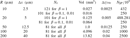
, because lower energy ions greatly increase the duration of simulation runs. The other simulation parameters are summarized in table 1. The grid spacing is chosen in the simulations with the three smallest grains according to
 $R/{\rm\Delta}x=4$
and to
 $R/{\rm\Delta}x=5$
for the others. The spherical surface is then represented by 206 or 270 grid points, respectively. The simulation time steps
 ${\rm\Delta}t$
are chosen to satisfy the Courant–Friedrichs–Lewy condition.
A magnetized plasma is created by overlapping the simulation box with a homogeneous and constant magnetic field in the
 $z$
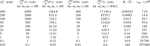
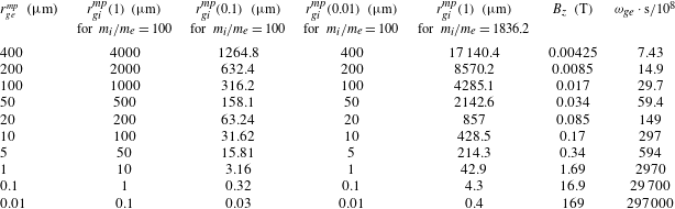
-direction. Ten different magnetic field strengths have been considered according to a most probable gyroradius (2.4) for electrons of smaller, similar or larger size than the grain radii and the Debye length. Table 2 summarizes the magnetic field strengths
 $B_{z}$
, the corresponding most probable gyroradius for ions/electrons and electron frequency of gyration, given by
 ${\it\omega}_{ge}=e^{}B_{z}/m_{e}$
. The magnetic field strengths cover the spectrum from moderate levels up to very strong fields of
 $169~\text{T}$
.
All simulations are started with a uniform Maxwellian plasma and the system develops self-consistently until the dust charge and shielding potential around the grain reaches a steady state. At the equilibrium state, the dust charge fluctuates due to collection of plasma particles and an average over a sufficiently large time interval (several tens of
 ${\it\omega}_{ge}$
) is considered. The dust charge fluctuations are very small, the standard deviation is only approximately
 $10^{-3}$
. Depending on the number of grid points and the parameters a simulation run is between 20 and 200 h with an Intel Core I7–3770 K
 $4\times 3.5~\text{GHz}$
processor.
Parameters of the OPAR simulations.
 $R$
is the dust grain radius,
 ${\rm\Delta}x$
the grid spacing,
 $N_{x}$
the number of grid points per side of the cubic simulation box, Vol the physical volume of the box (including the dust grain),
 ${\rm\Delta}t$
the time step and
 $N_{SP}$
the initial number of ions/electrons in the simulation.

Parameters of the OPAR simulations for magnetized plasmas.
 $r_{ge}^{mp}$
is the electron most probable gyroradius,
 $r_{gi}^{mp}({\it\beta})$
the ion most probable gyroradius depending on the temperature ratio
 ${\it\beta}$
,
 $B_{z}$
the magnetic field strength and
 ${\it\omega}_{ge}$
electron frequency of gyration.
4. Results
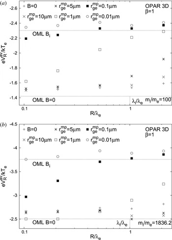
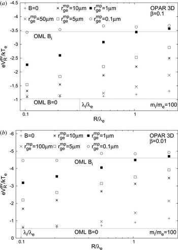
In figures 3 and 4 the time averaged surface potentials
 ${\it\eta}_{R}^{av}$
at the equilibrium state of the five grains are shown for different magnetic field strengths and for three plasma temperature ratios
 ${\it\beta}$
, respectively. Figure 3 shows the case for
 ${\it\beta}=1$
and the two mass ratios. The standard deviation is always very low (
 $10^{-3}$
) and can be neglected in comparison to the drawing accuracy. The lower horizontal lines (OML
 $B=0$
) represent results from the unmodified OML theory without a magnetic field (2.3) and the upper horizontal lines (OML
 $B_{i}$
) are from the fully magnetized case according to (2.7). The vertical lines mark the ion Debye length and determine the transition between the OML and OM case. For comparison, the upright crosses are the results of simulations without a magnetic field and with small grains and are in good agreement with the unmodified OML theory with a relative difference of approximately
 $+5\,\%$
. This difference is caused by the ratio of the grain radius to the grid distance. A larger ratio (smaller
 ${\rm\Delta}x$
) results in a more accurate potential, but requires higher numerical effort. In all following simulation results this systematic error has to be taken into account.
With decreasing gyroradius (increasing magnetic field strength) the surface potentials become more negative for all grains. A significant change can be found depending on the temperature ratio when the electron most probable gyroradius becomes considerably smaller than its Debye length. For very high magnetic field strengths (small gyroradius) the surface potentials tend for all grains to the modified OML theory of the fully magnetized case. However, the increase in the surface potential with decreasing gyroradius has a larger effect for larger grains. The absolute value of the surface potential is not directly dependent on the magnetic field strength, but on the ratio
 ${\it\gamma}_{i}$
or
 ${\it\gamma}_{e}$
, which is illustrated in figures 5 and 6.
Time-averaged surface potentials
 ${\it\eta}_{R}^{av}=e^{}V_{R}^{av}/kT_{e}$
at the equilibrium state of the five grains for different magnetic field strengths (expressed here by electron most probable gyroradius
 $r_{ge}^{mp}$
), for the temperature ratio
 ${\it\beta}=T_{i}/T_{e}=1$
and two mass ratios. The upright crosses are results of simulations without a magnetic field. The lower horizontal lines (OML
 $B=0$
) represent results from the unmodified OML theory (2.3) and the upper horizontal lines (OML
 $B_{i}$
) from the fully magnetized case (2.7). The vertical lines mark the ion Debye length and determine the transition between OML and OM case.

Time-averaged surface potentials
 ${\it\eta}_{R}^{av}=e^{}V_{R}^{av}/kT_{e}$
at the equilibrium state of the five grains for different magnetic field strengths (expressed here by electron most probable gyroradius
 $r_{ge}^{mp}$
), for two temperature ratios
 ${\it\beta}=T_{i}/T_{e}$
and the mass ratio of
 $100$
. The upright crosses are results of simulations without a magnetic field. The lower horizontal lines (OML
 $B=0$
) represent results from the unmodified OML theory (2.3) and the upper horizontal lines (OML
 $B_{i}$
) from the fully magnetized case (2.7). The vertical lines mark the ion Debye length and determine the transition between OML and OM case.

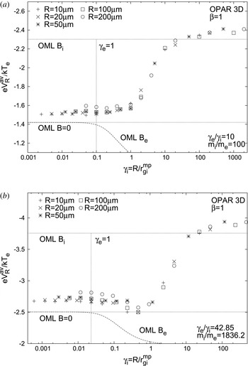
Time-averaged surface potentials
 ${\it\eta}_{R}^{av}=e^{}V_{R}^{av}/kT_{e}$
at the equilibrium state of the five grains depending on the ratio
 ${\it\gamma}_{i}=R/r_{gi}^{mp}$
, for the temperature ratio
 ${\it\beta}=T_{i}/T_{e}=1$
and two mass ratios. The lower horizontal lines (OML
 $B=0$
) represent results from the unmodified OML theory (2.3) and the upper lines (OML
 $B_{i}$
) from the fully magnetized case (2.7). The dotted decreasing curve (OML
 $B_{e}$
) represents the modified OML theory (2.5) for the case of a magnetized electron but unmagnetized ion current (2.5).

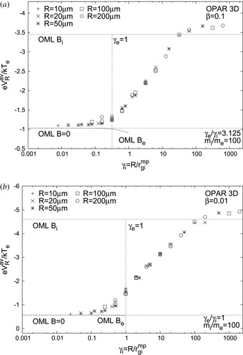
Time-averaged surface potentials
 ${\it\eta}_{R}^{av}=e^{}V_{R}^{av}/kT_{e}$
at the equilibrium state of the five grains depending on the ratio
 ${\it\gamma}_{i}=R/r_{gi}^{mp}$
, for two temperature ratios
 ${\it\beta}=T_{i}/T_{e}$
and the mass ratio of
 $100$
. The lower horizontal lines (OML
 $B=0$
) represent results from the unmodified OML theory (2.3) and the upper lines (OML
 $B_{i}$
) from the fully magnetized case (2.7). The dotted decreasing curve (OML
 $B_{e}$
) represents the modified OML theory (2.5) for the case of a magnetized electron but unmagnetized ion current (2.5).

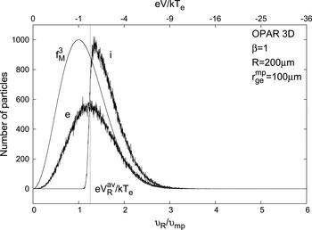
Velocity distribution of the grain absorbed ions (i) and electrons (e) in a simulation with the parameters as indicated at the top right. Each of the two distributions includes approx.
 $270\,000$
particles, which were absorbed in a period of
 $2400\,{\it\omega}_{e}$
after the equilibrium state was reached.
 $v_{R}$
is the particles velocity on the grain surface and
 $v_{mp}$
is the most probable velocity according to Maxwell. The normalised velocity
 $v_{R}/v_{mp}$
is expressed in the upper axis by the energy according to (4.1). For comparison, an undisturbed Maxwell distribution (
 $\,f_{M}^{3}$
) is shown. The vertical line is the time-averaged surface potential
 $e^{}V_{R}^{av}/kT_{e}$
of the grain in its equilibrium state.

Figures 5 and 6 show the time-averaged surface potentials
 ${\it\eta}_{R}^{av}$
at the equilibrium state depending on the ratio
 ${\it\gamma}_{i}=R/r_{gi}^{mp}$
for all magnetized plasma simulations performed. Figure 5 shows the case for
 ${\it\beta}=1$
and the two mass ratios. The dotted decreasing curve (OML
 $B_{e}$
) represents the modified OML theory (2.5) for the case of a magnetized electron but unmagnetized ion current in the range
 ${\it\gamma}_{i}<1<{\it\gamma}_{e}$
. The dependency of
 ${\it\gamma}_{i}$
is according to Patacchini, Hutchinson & Lapenta (Reference Patacchini, Hutchinson and Lapenta2007), in which electron currents to a sphere in a magnetized plasma are found and modelled by numerical integration of sufficient numbers of particle trajectories. Because the mass ratio is only
 $100$
, the most probable gyroradius of the ions and electrons match (
 ${\it\gamma}_{i}={\it\gamma}_{e}$
) for the lowest temperature ratio
 ${\it\beta}=0.01$
. For
 ${\it\gamma}_{i}>1$
the potentials become increasingly negative and the absolute value becomes independent of the grain radius
 $R$
. Obviously, the surface potentials are not decreasing for
 ${\it\gamma}_{i}<1<{\it\gamma}_{e}$
in the manner predicted by the modified OML theory, independent of the temperature or mass ratio. For
 ${\it\beta}=1$
only a little decrease occurs for the largest grain (upper panel) and for the higher mass ratio, the decrease is more significant for all grains (lower panel), but no correlation with the curve OML
 $B_{e}$
can be found. In the range of
 ${\it\gamma}_{i}<1<{\it\gamma}_{e}$
the electron charging current begins to decrease significantly (in comparison to the case without a magnetic field), but the ion current decreases also and even more than that of the electrons, because the surface potentials becomes more negative, although the most probable gyroradius of the ions is still larger than the grain radius
 $R$
. This effect is also present for lower energy ions, which means for lower temperature or higher mass ratios. In the modified OML approach for the case of a magnetized electron but unmagnetized ion current it was not taken into consideration that the kinetic energy of the plasma particles, and therefore their gyroradii, are affected in the central potential field of the grains. Due to the repulsive potential, electrons lose kinetic energy and the gyroradius decreases, whereas ions absorb kinetic energy due to the attractive potential and the gyroradius increases on the way to the grain.
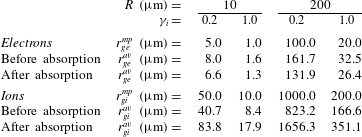
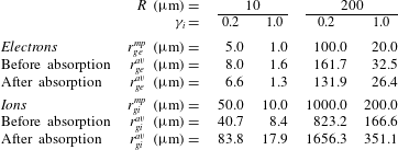
Gyroradii of electrons/ions in simulations with the largest and smallest grain radius at
 ${\it\beta}=1$
.
 $r_{ge}^{mp}$
and
 $r_{gi}^{mp}$
are the most probable gyroradii, set as default values in the simulations.
 $r_{ge}^{av}$
and
 $r_{gi}^{av}$
are averaged gyroradii from the velocity distributions of absorbed particles at the grain (line after absorption) and from the undisturbed Maxwell distribution of those particles, which contributes to the charging current (line before absorption).
To what extent the gyroradius of the arriving ions/electrons is changed can be analysed with the velocity distribution of the absorbed particles. Figure 7 shows the velocity distribution of absorbed ions (i) and electrons (e) in the simulation with the parameters
 $R=200~{\rm\mu}\text{m}$
,
 ${\it\beta}=1$
,
 $m_{i}/m_{e}=100$
and
 $r_{ge}^{mp}=100~{\rm\mu}\text{m}$
.
 $v_{R}$
is the velocity on the grain surface and
 $v_{mp}$
the most probable velocity according to Maxwell. Each of the two velocity distributions includes approximately
 $270\,000$
particles, which were absorbed at the grain and removed from the simulation in a period of
 $2400{\it\omega}_{e}$
after the grain has reached its equilibrium state. The normalised velocity
 $v_{R}/v_{mp}$
can also be expressed by the energy (potential)
 $e^{}V_{R}/kT_{e}$
:
 $$\begin{eqnarray}\left(\frac{v_{R}}{v_{mp}}\right)^{2}=\frac{\frac{1}{2}mv_{R}^{2}}{kT_{e}}=\frac{e^{}V_{R}}{kT_{e}},\end{eqnarray}$$
see the upper axis in figure 7. For comparison, an undisturbed Maxwell distribution (
 $\,f_{M}^{3}$
) is shown. The vertical line is the time-averaged surface potential
 $e^{}V_{R}^{av}/kT_{e}$
of the grain in its equilibrium state. The distribution of the ions rises rapidly near the surface potential, because ions collect this energy at a minimum on the way through the attractive potential. The distribution of electrons has a maximum at this point. The averaged velocity of the two distributions are
 $v_{av}^{i}=1.67v_{mp}^{i}$
for ions and
 $v_{av}^{e}=1.33v_{mp}^{e}$
for electrons. Consequently an averaged gyroradius can be defined by
 $$\begin{eqnarray}r_{g}^{av}=\frac{mv_{av}}{2e^{}B_{z}},\end{eqnarray}$$
see (2.4). In table 3 the corresponding averaged gyroradii are listed for the above-mentioned simulation and furthermore, for simulations with the smallest grain radius as well as for simulations with
 ${\it\gamma}_{i}=0.2$
and
 ${\it\gamma}_{i}=1$
. For comparison, the averaged gyroradii of those ions/electrons from an undisturbed Maxwell distribution are shown, which contributes to the charging current. Only electrons with sufficient energy to overcome the retarding potential can be absorbed by the grain, represented by the right part of the Maxwell distribution in figure 7, separated by the vertical line
 $e^{}V_{R}^{av}/kT_{e}$
. In contrast, the major part of the absorbed ions have originally a lower energy in comparison to the surface potential, represented by the left part of the Maxwell distribution. From these two parts, averaged velocities and gyroradii follow according to (4.2). For all four simulations shown in table 3 the electron averaged gyroradius has decreased by approximately 20 % in comparison to the original averaged gyroradius, but is still larger by approximately 30 % than the most probable gyroradius. Ion averaged gyroradius has almost doubled on the way to the grain in comparison to the original averaged gyroradius. In comparison to the most probable gyroradius, it has increased by approximately 70 %.
An interesting fact is that the relative increase/decrease of the ions/electrons gyroradii is independent of the magnetic field strength, the ratios
 ${\it\gamma}_{i}$
,
 ${\it\gamma}_{e}$
or the Debye lengths. For the simulations with
 ${\it\gamma}_{i}=0.2$
the electron gyroradius is always lower than the grain radius, for the largest as well as for the smallest grain, for which reason the magnetized electron charging current is hardly affected. In contrast, the ion gyroradii are always larger than the grain radius, but have been almost doubled due to energy collection in the potential field. The strong increase of the ion gyroradius results in a reduced charging current, because arriving ions with a certain phase angle of the spiral motion can miss the spherical grain surface. Very similar results as those given in table 3 were achieved for the higher mass ratio of hydrogen. In fact, the ions gyroradii are than much larger than for the lower ion mass, but also the equilibrium surface potentials of the dust grains are more negative (see figure 1), which means that the ions are absorbing much more kinetic energy on the way to the grain in comparison to the case of a lower ion mass. Because of this, the relation of the averaged gyroradii before and after absorption are the same as for the lower mass ratio. The decrease of ion charging current is stronger than that of the electrons in a magnetized plasma for all grain radii, even though ions highest gyroradius is larger than the grain radius (
 ${\it\gamma}_{i}<1$
). These conditions are not considered in the modified OML approach. Although the most probable electron gyration radius is always smaller than that of ions in a Maxwellian plasma, a simultaneous situation of magnetized electron and unmagnetized ion charging current never exists. This behaviour was also supposed by Patacchini et al. (Reference Patacchini, Hutchinson and Lapenta2007) for small grains in comparison to the plasma Debye length and mass ratios of hydrogen and argon by using the hybrid PIC code SCEPTIC.
5. Summary
The charging currents to an object or dust grain are significantly affected in a magnetized plasma, because in a magnetic field the movements of the plasma particles are forced into spiral orbits. With the fully 3-D PIC code OPAR we have investigated the surface potential at the equilibrium state of dust grains with different sizes in comparison to the plasma Debye length and the ions/electrons gyroradius. The surface potential of the dust grains at the equilibrium state become more negative with increasing magnetic field strength or decreasing gyroradius and has only a dependence on the ratio
 ${\it\gamma}_{i},{\it\gamma}_{e}$
and not directly on the magnetic field strength.
In a Maxwellian plasma, the most probable gyroradius of the electrons is smaller than that of ions, but in the range of
 ${\it\gamma}_{i}<1<{\it\gamma}_{e}$
the charging current of the ions is also reduced significantly. This effect is independent of the temperature or mass ratios. Therefore, a simultaneous situation of magnetized electron and unmagnetized ion charging currents never exists in a Maxwellian plasma, as suggested by Tsytovich et al. (Reference Tsytovich, Sato and Morfill2003). In this modified OML approach it was not taken into consideration that the plasma particle gyroradius is affected by a change of kinetic energy in the central potential field of the grains. With the velocity distribution of the absorbed particles it was shown that the ion average gyroradius was almost doubled on the way to the grain in comparison to the original averaged gyroradius, while the decrease in the electron average gyroradius is rather small. The relative increase/decrease of ions/electrons gyroradius is independent of the magnetic field strength, the grain radius, the ratio
 ${\it\gamma}_{i},{\it\gamma}_{e}$
or the Debye lengths. The strong increase of the ion gyroradius results in a reduced charging current and therefore in a more negative surface potential, because arriving ions with a certain phase angle of spiral motion can miss the grain. The decrease of ion charging current is stronger than that of electrons in a magnetized plasma for all grain radii, even though the ion most probable gyroradius is larger than the grain radius.
However, the modified OML approach for the fully magnetized case of Tsytovich et al. (Reference Tsytovich, Sato and Morfill2003) is a good approximation if the gyroradius is very small (
 ${\it\gamma}_{i},{\it\gamma}_{e}\gg 1$
) and the particles can be considered to be moving along the magnetic field lines and straight towards the grain. Nonetheless, this situation only occurs for very high magnetic field strengths, see table 2. Future work will be focused on the investigation of dust grain clusters in magnetized plasmas with OPAR simulations.
Acknowledgement
The author wish to thank Professor Dr R. Grauer for supporting this work and the resulting dissertation.