1. Introduction
Determining the energy balance for the ocean remains an important problem with implications for the global circulation and long term variability (Penduff et al. Reference Penduff, Juza, Barnier, Zika, Dewar, Treguier, Molines and Audiffren2011). Since an understanding of interannual to centennial variability is required for climate predictions, an accurate model for the ocean energy budget is vital for addressing climate change (Stocker et al. Reference Stocker, Qin, Plattner, Tignor, Allen, Boschung, Nauels, Xia, Bex and Midgley2013). Much of the kinetic energy in the ocean resides within mesoscale features, balanced motions with horizontal length scales of the order of 10–100 km (Ferrari & Wunsch Reference Ferrari and Wunsch2009). The processes by which mesoscales are energised by large scale winds are fairly well understood. However, the balanced motion of mesoscales, which act to transfer energy to larger scales, cannot fully account for this energy uptake. This suggests that significant amounts of energy are being lost to small scale, unbalanced motions (Dewar, Berloff & Hogg Reference Dewar, Berloff and Hogg2011). This dissipation of mesoscale energy occurs on scales that are not typically resolved by global ocean simulations; hence, a physically motivated parametrisation is required to describe the effects of these processes.
Internal waves are a candidate for the extraction of mesoscale energy; however, their spontaneous generation within the ocean interior is weak (Vanneste & Yavneh Reference Vanneste and Yavneh2004; Shakespeare & Hogg Reference Shakespeare and Hogg2017) suggesting that they are not the primary mechanism for energy transfer. A second candidate is submesoscale motions where the term ‘submesoscale’ refers to processes occurring on horizontal scales from 100 m to 10 km which are characterised by order-unity Rossby numbers (Thomas, Tandon & Mahadevan Reference Thomas, Tandon and Mahadevan2008; McWilliams Reference McWilliams2016). These partially unbalanced motions have been observed near the ocean surface and boundaries and can form a forward cascade where energy is transferred to increasingly small scales and eventually dissipated by turbulent mixing (Capet et al. Reference Capet, McWilliams, Molemaker and Shchepetkin2008a,Reference Capet, McWilliams, Molemaker and Shchepetkinb; D'Asaro et al. Reference D'Asaro, Lee, Rainville, Harcourt and Thomas2011). Therefore submesoscale processes occurring near the ocean surface and boundaries are likely to be important for determining the mesoscale energy loss (Arbic et al. Reference Arbic, Shriver, Hogan, Hurlburt, McClean, Metzger, Scott, Sen, Smedstad and Wallcraft2009; Dewar et al. Reference Dewar, Berloff and Hogg2011; McWilliams Reference McWilliams2016). Other potentially important effects for the energy budget include the relative wind stress at the ocean surface (Duhaut & Straub Reference Duhaut and Straub2006), deep-ocean bottom drag (Sen, Scott & Arbic Reference Sen, Scott and Arbic2008) and topographic lee wave generation (Nikurashin & Ferrari Reference Nikurashin and Ferrari2010).
An important feature of submesoscales is an elevated level of small scale turbulence (D'Asaro et al. Reference D'Asaro, Lee, Rainville, Harcourt and Thomas2011; Callies et al. Reference Callies, Ferrari, Klymak and Gula2015, Reference Callies, Flierl, Ferrari and Fox-Kemper2016; Mashayek et al. Reference Mashayek, Ferrari, Merrifield, Ledwell, St. Laurent and Naveira Garabato2017), generated by a variety of processes including boundary forcing, bottom drag, internal wave breaking and shear instabilities (Large, McWilliams & Doney Reference Large, McWilliams and Doney2011). Turbulence acts to transfer energy down scale until it is dissipated by viscous forces at the Kolmogorov scale (Vassilicos Reference Vassilicos2015). This turbulent mixing plays an significant role in various processes such as frontogenesis (Gula, Molemaker & McWilliams Reference Gula, Molemaker and McWilliams2014; McWilliams Reference McWilliams2017; Crowe & Taylor Reference Crowe and Taylor2018, Reference Crowe and Taylor2019b), restratification (Fox-Kemper, Ferrari & Hallberg Reference Fox-Kemper, Ferrari and Hallberg2008) and submesoscale instabilities in the surface mixed layer (Young & Chen Reference Young and Chen1995; Skyllingstad & Samelson Reference Skyllingstad and Samelson2012; Crowe & Taylor Reference Crowe and Taylor2019a) where it is commonly parametrised using an eddy viscosity (Large et al. Reference Large, McWilliams and Doney2011). Due to the small vertical scales of submesoscale processes – which are usually of the order of 10–100 m – vertical mixing is especially important.
In addition to determining global energy balances, recent work has highlighted the importance of understanding the processes which govern the sources and sinks of mesoscale eddy energy for the development of eddy parametrisations (Marshall & Adcroft Reference Marshall and Adcroft2010; Jansen et al. Reference Jansen, Adcroft, Khani and Kong2019; Poulsen et al. Reference Poulsen, Jochum, Maddison, Marshall and Nuterman2019). Bachman (Reference Bachman2019), for example, parameterised the backscatter of eddy energy to the mean flow by modelling the transfer of potential energy to kinetic energy by baroclinic turbulence. A theoretical understanding of the processes unresolved by global ocean models is thus essential for the formulation of physically motivated eddy parametrisations.
While there has been much work focusing on submesoscale processes near the ocean surface, submesoscale generation near the bottom and lateral boundaries has been much less studied. Work by Dewar et al. (Reference Dewar, Berloff and Hogg2011) and Gula, Molemaker & McWilliams (Reference Gula, Molemaker and McWilliams2016) has shown that walls and bottom topography can also generate submesoscale features which may provide a significant sink of interior mesoscale energy. The processes and energy pathway are, however, poorly understood.
Recently, Deremble, Johnson & Dewar (Reference Deremble, Johnson and Dewar2017) derived a simple model which coupled large scale interior quasi-geostrophic motion with the boundary response due to vertical walls. They demonstrated a close agreement with high resolution primitive equation simulations and argued that boundary dynamics naturally dissipates balanced energy so represents a means of closing the oceanic mesoscale energy budget. The submesoscale response in this model was entirely captured by the Kelvin wave dynamics at the boundary (see also Dewar & Hogg Reference Dewar and Hogg2010; Hogg et al. Reference Hogg, Dewar, Berloff and Ward2011). An understanding of Kelvin waves in a regime where turbulent mixing, topography and nonlinearity all play an important role is therefore likely to be vital for accurately parametrising submesoscale boundary effects.
Unstratified shallow water models have been used extensively to study nonlinear wave dynamics. Smith (Reference Smith1972), for example, used a shallow water model to study the evolution of barotropic Kelvin waves along a straight coastline with offshore topography. Topography was shown to generate weak dispersion and to modify the non-dispersive wave speed. This topographic dispersion was balanced by nonlinear effects allowing the existence of solitary wave solutions. Later, Boyd (Reference Boyd1980) considered the nonlinear evolution of equatorial Kelvin waves using a shallow water model. The wave amplitude was found to satisfy Hopf's equation with breaking wave solutions that may be relevant to El Niño events in the equatorial Pacific ocean.
When studying baroclinic Kelvin waves, solutions are often expanded in terms of an infinite sum of linearly independent vertical modes as discussed for a general stratified ocean layer by McCreary & Lighthill (Reference McCreary and Lighthill1981). In the linear, unforced problem, the amplitudes of each vertical mode can be easily determined by projecting the system onto the required mode. The inclusion of forcing terms such as vertical mixing, topography and nonlinearity, however, couples these modes so the amplitudes of each mode cannot be independently determined. Martinsen & Weber (Reference Martinsen and Weber1981) and Davey, Hsieh & Wajsowicz (Reference Davey, Hsieh and Wajsowicz1983) considered linear baroclinic Kelvin waves in the presence of vertical mixing by making the assumption that the vertical viscosity was depth dependent and inversely proportional to the background stratification profile. Under this assumption the vertical modes separate allowing simple solutions to be found. Vertical mixing was found to damp all horizontal wavenumbers equally while also modifying the speed and phase of the wave as well as the propagation direction in the case of high Prandtl number.
The effect of topography on shelf waves has been studied by Johnson & Rodney (Reference Johnson and Rodney2011) and Rodney & Johnson (Reference Rodney and Johnson2012, Reference Rodney and Johnson2014, Reference Rodney and Johnson2015) using both numerical and analytic approaches. It was shown that changes in topography can modify the speed of wave propagation and even prevent the propagation of long waves. In the case where short wave reflection is also not possible the wave energy was found to be transferred to small scale eddies.
Romea & Allen (Reference Romea and Allen1984) used an asymptotic approach to consider the action of bottom friction and topography on baroclinic Kelvin modes in the case of linear, long waves. Under the assumption that the Ekman number was small, solutions were presented for the limits of steep and shallow slopes with the effects of bottom friction and topography entering as a small correction to the classical Kelvin wave solution. In the steep-slope limit, topography was shown to modify the wave speed with the speed change determined by the slope gradient. In the case of a constant-slope gradient, the speed was found to be unchanged whereas a convex or concave slope were found to respectively increase or decrease the wave speed.
We proceed here using the asymptotic approach of Romea & Allen (Reference Romea and Allen1984) to determine the effects of vertical mixing, steep-slope topography and weak nonlinearity on Kelvin waves. We also relax the long wave assumption and allow superinertial solutions with short wavelengths. Martinsen & Weber (Reference Martinsen and Weber1981) showed that the barotropic mode is not influenced by vertical mixing and so we consider only baroclinic modes, making the rigid lid assumption of no surface displacement. While an asymptotic approach imposes restrictions on the maximum size of the turbulent Ekman number, slope gradient and Rossby number, it allows us to use mixing profiles, slope geometries and stratifications with arbitrary depth dependence. Since turbulent mixing acts on both the momentum and buoyancy we include both effects and allow the Prandtl number describing the ratio of the mixing rates to be arbitrary (Davey et al. Reference Davey, Hsieh and Wajsowicz1983).
We find that topography, mixing and nonlinearity all play an important role in the evolution of Kelvin waves by modifying the wave speed and offshore structure as well as the long time evolution of the amplitude. Vertical mixing acts to oppose nonlinear wave breaking, however, breaking solutions are shown to be possible if the nonlinearity is sufficiently strong. Using typical submesoscale ocean parameters we estimate that nonlinearity may play an important role in the evolution of Kelvin waves with low vertical mode number whereas modes with smaller vertical scales may be quickly damped by turbulent mixing.
We begin in § 4 by considering the case of linear Kelvin waves and derive asymptotic solutions for the pressure field, modified by vertical mixing and topographic effects. Various limits are discussed in relation to previous work. In § 5 we consider the full nonlinear problem and derive a nonlinear evolution equation for the amplitude. Solutions to this equation are discussed in § 6 and realistic values for the parameters are estimated in § 7. Finally we discuss our conclusions in § 8.
2. Set-up
We consider a rotating, incompressible fluid layer bounded above and below by rigid boundaries and rotating about the vertical ( $z$) axis. To describe the effects of varying density, we make the Boussinesq approximation by assuming that density variations are small compared to a reference value. Density variations are split into an imposed background stratification which is assumed to depend only on depth and an evolving buoyancy field. The buoyancy field is described by a single scalar equation and defined as
 $b=-g\rho '/\rho _0$ where
 $\rho _0$ is a reference density,
 $g$ is the gravitational acceleration and
 $\rho '$ describes departures from
 $\rho _0$ with
 $\rho ' \ll \rho _0$.
The coastline is represented by a sloping boundary applied at  $y = l$ where
 $y$ is the offshore coordinate and along-shore (
 $x$) variations in topography are assumed to occur on sufficiently large scales that we can take
 $l = l(z)$. Boundary conditions of vanishing normal velocity are applied at
 $y=l$. We note that imposing a sloping sidewall,
 $y = l(z)$, is equivalent to imposing a sloping bottom,
 $z = h(y)$. Here we use the sloping sidewall approach since, in steep-slope limit, (small
 $l'(z)$ or large
 $h'(y)$) mapping the surface
 $y = l(z)$ back to a vertical boundary is more straightforward than mapping
 $z = h(y)$ to either a vertical or horizontal wall. We also introduce a depth-independent background flow which we assume also varies over large scales and hence can be taken as constant. By the boundary condition at
 $y=l$, this background flow must be parallel to the coastline.
Finally, the effects of turbulent mixing on the velocity and buoyancy fields are described using vertical diffusion terms where the depth-dependent viscosity and diffusivity describe the bulk effects of the mixing. The turbulent viscosity  $\nu$ and turbulent diffusivity
 $\kappa$ can vary over several orders of magnitude but will typically be within the range of
 $10^{-4}\text {--}10^{-2}\ \textrm {m}^{2}\,\textrm {s}$ (Large et al. Reference Large, McWilliams and Doney2011) with the ratio of these quantities, the turbulent Prandtl number, being order 1 (Venayagamoorthy & Stretch Reference Venayagamoorthy and Stretch2010).
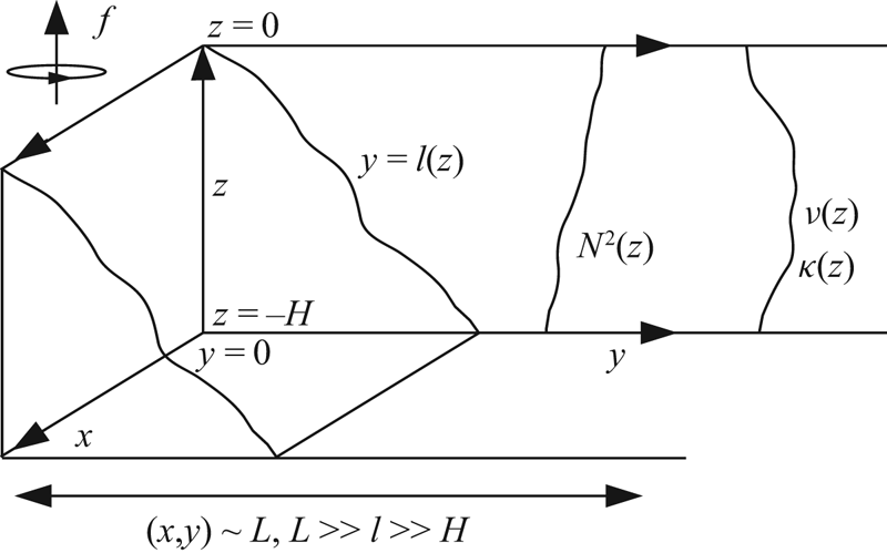
In order to isolate the effects of vertical mixing within the fluid layer, we neglect the bottom drag and associated bottom boundary layer by applying inviscid boundary conditions (Martinsen & Weber Reference Martinsen and Weber1981). The effects of bottom drag and Ekman pumping were extensively studied by Romea & Allen (Reference Romea and Allen1984) and so we return to this point in § 8. Our dimensional problem set-up is shown in figure 1.
The flow geometry with sloping boundary  $y=l(z)$, Coriolis parameter
 $f$, viscosity
 $\nu$, diffusivity
 $\kappa$ and stratification with vertical buoyancy gradient
 $N^2(z)$. The depth is given by
 $H$ while
 $L$ describes the typical scale of horizontal motion. A constant background flow,
 $U$, in the
 $x$ direction is also included.

We now non-dimensionalise the horizontal coordinates  $(x,y)$ by the Rossby radius of deformation
 $L_R = NH/f$, the vertical coordinate
 $z$ by the depth
 $H$, the horizontal velocity
 $(u,v)$ by a typical velocity scale
 $V$, the vertical velocity
 $w$ by
 $f\,V/N$, the buoyancy
 $b$ by
 $VN$, the pressure
 $p$ by
 $VNH$, the time
 $t$ by
 $1/f$, the along-shore background flow
 $U$ by
 $NH$ and the horizontal extent of the boundary
 $l$ by
 $L$. Here
 $N$ is the characteristic scale of the buoyancy frequency describing the vertical stratification and
 $f$ is the Coriolis parameter.
We define the Rossby number as  ${Ro} = V/(\,fL_R) = V/(NH)$ and write
 $\epsilon = \sqrt {f/N}$ so the ratio of the depth to the Rossby radius of deformation is given by
 $\epsilon ^2$. Finally we define the Ekman number by
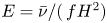 ${E} = \bar {\nu }/(\,fH^2)$ and Prandtl number by
 ${Pr} = \bar {\nu }/\bar {\kappa }$ where
 $\bar {\nu }$ and
 $\bar {\kappa }$ are characteristic scales for the turbulent viscosity and diffusivity respectively. We note that
 $\bar {\nu }$ and
 $\bar {\kappa }$ may be chosen as, for example, a depth-average or maximum value of
 $\nu$ and
 $\kappa$. Our non-dimensional equations are given by
 \begin{gather} \left[\frac{\partial }{\partial t}+U\frac{\partial }{\partial x}\right]u +{Ro} \left[ u\frac{\partial u}{\partial x}+v\frac{\partial u}{\partial y}+w\frac{\partial u}{\partial z} \right] - v = -\frac{\partial p}{\partial x} +{E}\, \mathcal{D}_u u, \end{gather}
 \begin{gather}\left[\frac{\partial }{\partial t}+U\frac{\partial }{\partial x}\right]v +{Ro} \left[ u\frac{\partial v}{\partial x}+v\frac{\partial v}{\partial y}+w\frac{\partial v}{\partial z} \right] + u = - \frac{\partial p}{\partial y} + {E}\, \mathcal{D}_u v, \end{gather}
 \begin{gather}\epsilon^4\left[\frac{\partial }{\partial t}+U\frac{\partial }{\partial x}\right]w +\epsilon^4{Ro} \left[ u\frac{\partial w}{\partial x}+v\frac{\partial w}{\partial y}+w\frac{\partial w}{\partial z} \right] = b-\frac{\partial p}{\partial z} + \epsilon^4{E}\, \mathcal{D}_u w, \end{gather}
 \begin{gather}\left[\frac{\partial }{\partial t}+U\frac{\partial }{\partial x}\right]b +{Ro} \left[ u\frac{\partial b}{\partial x}+v\frac{\partial b}{\partial y}+w\frac{\partial b}{\partial z} \right]= -\mathcal{N}^2 w + \frac{{E}}{{Pr}} \mathcal{D}_b b, \end{gather}
 \begin{gather}\frac{\partial u}{\partial x}+\frac{\partial v}{\partial y} +\frac{\partial w}{\partial z}= 0, \end{gather}
where  $\mathcal {N}^2 = \mathcal {N}^2(z)$ is the square of the buoyancy frequency non-dimensionalised by
 $N^2$, hence, in the case of constant buoyancy frequency, we can take
 $\mathcal {N}^2 = 1$. The vertical mixing terms are given by
 \begin{equation} \mathcal{D}_u = \frac{\partial }{\partial z} \left[ D_u \frac{\partial }{\partial z} \right], \quad \mathcal{D}_b = \frac{\partial }{\partial z} \left[ D_b \frac{\partial }{\partial z} \right], \end{equation}
where  $D_u = \nu (z)/\bar {\nu }$ and
 $D_b = \kappa (z)/\bar {\kappa }$ are order-
 $1$ functions of
 $z$ describing the vertical structure of the turbulent viscosity and diffusivity respectively. Our coastal boundary condition is
 \begin{equation} v = \epsilon^2 \frac{L}{H} \frac{\partial l}{\partial z} w\quad \textrm{at} \ y = \epsilon^2 \frac{Ll}{H}. \end{equation}
We now take  $\epsilon \ll 1$ and assume that
 $NH/f \gg L \gg H$ by taking
 $H/L = O(\epsilon )$. Therefore, the boundary extent
 $L l$ is small compared to the Rossby radius of deformation but large compared to the depth. We call this limit the ‘steep-slope’ limit due to the assumption of
 $L \ll L_R$ and note that
 $\epsilon$ describes the aspect ratio of the sloping boundary in the non-dimensional formulation as
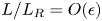 $L/L_R = O(\epsilon )$. Writing
 $\epsilon Ll/H = \delta (z) \sim O(1)$ we have
 \begin{equation} v = \epsilon \delta'(z) w\quad \textrm{at} \ y = \epsilon \delta(z), \end{equation}
where  $\delta '(z) = {\partial \delta }/{\partial z}$. This is the steep-slope boundary condition used by Romea & Allen (Reference Romea and Allen1984). On the top and bottom surfaces we make the rigid lid approximation that the vertical velocity vanishes
 \begin{equation} w = 0\quad \textrm{at} \ z=-1,0, \end{equation}
and we assume that perturbations do not grow as  $y \to \infty$.
3. Asymptotic analysis
We proceed by assuming that the Rossby and Ekman numbers are small by writing
 \begin{equation} ({Ro},{E}) = \epsilon(\mathcal{R},\mathcal{E}), \end{equation}
where we take  $\mathcal {E} \sim O(1)$ and consider two cases for
 $\mathcal {R}$: the linear case of
 $\mathcal {R} \ll 1$ and the weakly nonlinear case of
 $\mathcal {R} \sim O(1)$. Note that for typical ocean parameters we might expect
 ${E} \ll {Ro}$, however, we retain possible dissipative effects by assuming both are
 $O(\epsilon )$ and return to this point in § 7, where we find that, due to a difference in the size of the coefficient, both mixing and nonlinearity can be similar-order effects. Correct to
 $O(\epsilon )$ (2.1) can be written as
 \begin{gather} \left[\frac{\partial }{\partial t}+U\frac{\partial }{\partial x}\right]u +\epsilon\mathcal{R} F_u - v = -\frac{\partial p}{\partial x} +\epsilon\mathcal{E}\, \mathcal{D}_u u, \end{gather}
 \begin{gather}\left[\frac{\partial }{\partial t}+U\frac{\partial }{\partial x}\right]v +\epsilon\mathcal{R} F_v + u = - \frac{\partial p}{\partial y} + \epsilon\mathcal{E}\, \mathcal{D}_u v, \end{gather}
 \begin{gather}0 = b -\frac{\partial p}{\partial z}, \end{gather}
 \begin{gather}\left[\frac{\partial }{\partial t}+U\frac{\partial }{\partial x}\right]b +\epsilon\mathcal{R} F_b = -\mathcal{N}^2 w + \frac{\epsilon\mathcal{E}}{{Pr}}\, \mathcal{D}_b b, \end{gather}
 \begin{gather}\frac{\partial u}{\partial x}+\frac{\partial v}{\partial y} +\frac{\partial w}{\partial z} = 0, \end{gather}
where we note that the vertical momentum equation has reduced to hydrostatic balance and the nonlinear forcing terms are given by
 \begin{align} F_u = u\frac{\partial u}{\partial x}+v\frac{\partial u}{\partial y}+w\frac{\partial u}{\partial z}, \quad F_v = u\frac{\partial v}{\partial x}+v\frac{\partial v}{\partial y}+w\frac{\partial v}{\partial z}, \quad F_b = u\frac{\partial b}{\partial x}+v\frac{\partial b}{\partial y}+w\frac{\partial b}{\partial z}. \end{align}
Defining advection–diffusion operators as
 \begin{equation} \mathcal{L}_u = \left[\frac{\partial }{\partial t} + U \frac{\partial }{\partial x} - \epsilon \mathcal{E} \frac{\partial }{\partial z}\left(D_u(z) \frac{\partial }{\partial z}\right)\right], \end{equation}
and
 \begin{equation} \mathcal{L}_b = \left[\frac{\partial }{\partial t} + U \frac{\partial }{\partial x} - \frac{\epsilon\mathcal{E}}{{Pr}} \frac{\partial }{\partial z}\left(D_b(z) \frac{\partial }{\partial z}\right)\right], \end{equation}
we can write (3.2) as
 \begin{gather} (1+\mathcal{L}_u^2) u = -\left(\frac{\partial p}{\partial y} +\mathcal{L}_u\frac{\partial p}{\partial x}\right) - \epsilon\mathcal{R}\left(F_v+\mathcal{L}_u F_u\right), \end{gather}
 \begin{gather}(1+\mathcal{L}_u^2) v = \left(\frac{\partial p}{\partial x}-\mathcal{L}_u\frac{\partial p}{\partial y}\right)+ \epsilon\mathcal{R}(F_u - \mathcal{L}_u F_v), \end{gather}
 \begin{gather}w = -\frac{1}{\mathcal{N}^2} \left[ \mathcal{L}_b \frac{\partial p}{\partial z} + \epsilon\mathcal{R} F_b \right], \end{gather}
 \begin{gather}b = \frac{\partial p}{\partial z}, \end{gather}
which can be combined using mass conservation to give an equation for the pressure forced by the nonlinear terms. We have
 \begin{align} &(1+\mathcal{L}_u^2) \frac{\partial }{\partial z}\left[\frac{1}{\mathcal{N}^2}\mathcal{L}_b\frac{\partial p}{\partial z}\right] + \mathcal{L}_u\left(\frac{\partial ^2}{\partial x^2} + \frac{\partial ^2}{\partial y^2}\right)p \nonumber\\ &\quad = -\epsilon\mathcal{R} \left[ -\left(\frac{\partial F_u}{\partial y}-\frac{\partial F_v}{\partial x}\right) + \mathcal{L}_u \left( \frac{\partial F_u}{\partial x}+\frac{\partial F_v}{\partial y}\right) + (1+\mathcal{L}_u^2) \frac{\partial }{\partial z}\left[\frac{F_b}{\mathcal{N}^2}\right] \right], \end{align}
subject to
 \begin{equation} \mathcal{L}_b\frac{\partial p}{\partial z} = -\epsilon\mathcal{R} F_b\quad \textrm{at} \ z=-1,0, \end{equation}
and
 \begin{equation} \frac{\partial p}{\partial x} - \mathcal{L}_u\frac{\partial p}{\partial y} = -\epsilon(1+\mathcal{L}_u^2)\left[ \frac{\delta'}{\mathcal{N}^2} \mathcal{L}_b \frac{\partial p}{\partial z} \right] - \epsilon\mathcal{R}(F_u - \mathcal{L}_u F_v)\quad \textrm{at} \ y = \epsilon\delta, \end{equation}
correct to  $O(\epsilon )$. Note that in the case of
 $\epsilon = 0$ this reduces to the classical Kelvin wave problem.
Following Romea & Allen (Reference Romea and Allen1984) we define  $\lambda$ to be the offshore distance from the coastal boundary and perform the coordinate transformation
 \begin{equation} \lambda = y - \epsilon\delta(z), \end{equation}
where derivatives transform as
 \begin{equation} \frac{\partial }{\partial y} \to \frac{\partial }{\partial \lambda},\quad \frac{\partial }{\partial z} \to \frac{\partial }{\partial z}-\epsilon\delta' \frac{\partial }{\partial \lambda}. \end{equation}
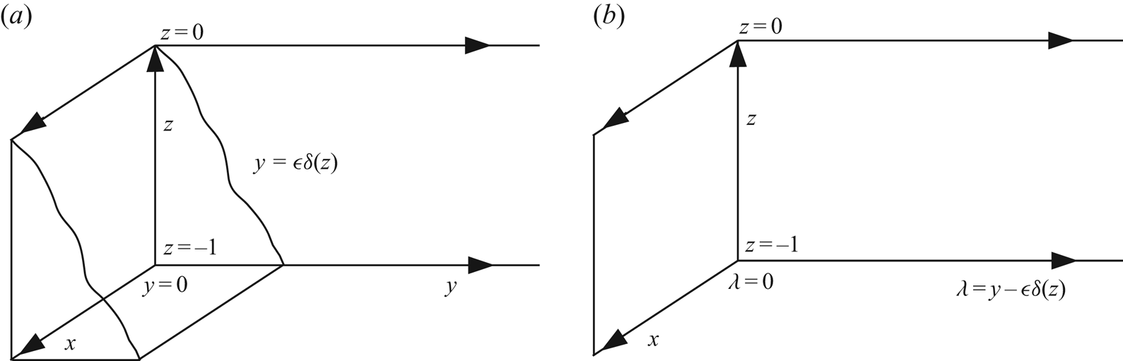
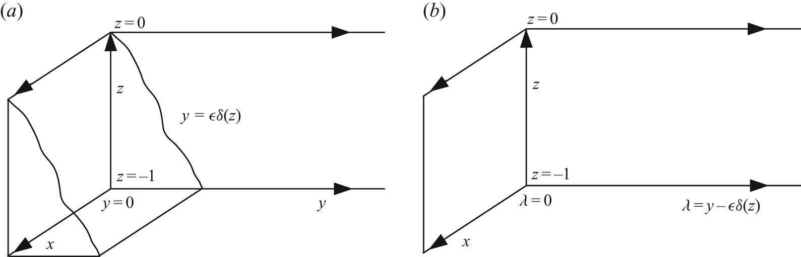
The effect of this transformation is to map the sloping wall  $y = \epsilon \delta (z)$ to a vertical boundary. Therefore the transformed slope boundary condition are applied at
 $\lambda = 0$ and the effects of the slope enter as new terms in the governing equations. Figure 2 shows the dimensionless geometry of the original and transformed domains. Equation (3.7) can now be written correct to
 $O(\epsilon )$ as
 \begin{align} &(1+\mathcal{L}_u^2) \left(\frac{\partial }{\partial z}-\epsilon\delta' \frac{\partial }{\partial \lambda}\right)\left[\frac{1}{\mathcal{N}^2}\mathcal{L}_b\left(\frac{\partial p}{\partial z}-\epsilon\delta' \frac{\partial p}{\partial \lambda}\right)\right] + \mathcal{L}_u\left(\frac{\partial ^2}{\partial x^2} + \frac{\partial ^2}{\partial \lambda^2}\right)p \nonumber\\ &\quad= -\epsilon\mathcal{R} \left[ -\left(\frac{\partial F_u}{\partial \lambda}-\frac{\partial F_v}{\partial x}\right) + \mathcal{L}_u \left( \frac{\partial F_u}{\partial x}+\frac{\partial F_v}{\partial \lambda}\right) + (1+\mathcal{L}_u^2) \frac{\partial }{\partial z}\left[\frac{F_b}{\mathcal{N}^2}\right] \right], \end{align}
subject to
 \begin{equation} \mathcal{L}_b\left(\frac{\partial p}{\partial z}-\epsilon\delta' \frac{\partial p}{\partial \lambda}\right) = -\epsilon\mathcal{R} F_b\quad \textrm{at} \ z=-1,0, \end{equation}
and
 \begin{equation} \frac{\partial p}{\partial x} - \mathcal{L}_u\frac{\partial p}{\partial \lambda} = -\epsilon(1+\mathcal{L}_u^2)\left[ \frac{\delta'}{\mathcal{N}^2} \mathcal{L}_b \frac{\partial p}{\partial z}\right] - \epsilon\mathcal{R}(F_u - \mathcal{L}_u F_v)\quad \textrm{at} \ \lambda = 0. \end{equation}
We note that  $\mathcal {L}_u$ and
 $\mathcal {L}_b$ only contain
 $\lambda$ derivatives at
 $O(\epsilon ^2)$ or higher so here are unchanged from (3.4) and (3.5).
(a) The dimensionless set-up in  $(x,y,z)$ space. The boundary conditions are applied at
 $z = -1, 0$ and
 $y = \epsilon \delta (z)$. (b) The dimensionless set-up in
 $(x,\lambda ,z)$ space where the boundary conditions are applied at
 $z = -1, 0$ and
 $\lambda = 0$.
Our model can be viewed as an extension of the steep-slope model of Romea & Allen (Reference Romea and Allen1984) and differs through the inclusion of vertical mixing and weak nonlinearity and the neglect of the bottom Ekman layer. Additionally we have relaxed the long wave assumption by taking both  $x$ and
 $y$ derivatives to be
 $O(1)$. Taking
 $\mathcal {E} = \mathcal {R} = 0$ and assuming a long wave limit recovers the steep-slope model considered by Romea & Allen (Reference Romea and Allen1984) in the case of vanishing bottom drag. Similarly, taking
 $\mathcal {R} = \delta = 0$ and
 $\mathcal {D}_u = \mathcal {D}_b = 1/\mathcal {N}^2$ recovers the vertical mixing model of Martinsen & Weber (Reference Martinsen and Weber1981) and Davey et al. (Reference Davey, Hsieh and Wajsowicz1983) where Martinsen & Weber (Reference Martinsen and Weber1981) also assumed that
 ${Pr} \to \infty$.
We now consider two cases: the linear case of  $\mathcal {R} \ll 1$ and the weakly nonlinear case of
 $\mathcal {R} = O(1)$.
4. The linear problem
We begin by considering the case of very small Rossby number,  ${Ro} \ll \epsilon$, by setting
 $\mathcal {R} = 0$. In this case the nonlinear terms in (3.12)–(3.14) vanish and the pressure field satisfies the linear problem
 \begin{equation} (1+\mathcal{L}_u^2) \left(\frac{\partial }{\partial z}-\epsilon\delta' \frac{\partial }{\partial \lambda}\right)\left[\frac{1}{\mathcal{N}^2}\mathcal{L}_b\left(\frac{\partial p}{\partial z}-\epsilon\delta' \frac{\partial p}{\partial \lambda}\right)\right] + \mathcal{L}_u\left(\frac{\partial ^2}{\partial x^2} + \frac{\partial ^2}{\partial \lambda^2}\right)p = 0, \end{equation}
subject to
 \begin{equation} \frac{\partial p}{\partial z}=\epsilon\delta' \frac{\partial p}{\partial \lambda}\quad \textrm{at} \ z=-1,0, \end{equation}
and
 \begin{equation} \frac{\partial p}{\partial x} - \mathcal{L}_u\frac{\partial p}{\partial \lambda} = -\epsilon(1+\mathcal{L}_u^2)\left[ \frac{\delta'}{\mathcal{N}^2} \mathcal{L}_b \frac{\partial p}{\partial z}\right]\quad \textrm{at} \ \lambda = 0. \end{equation}
Following Romea & Allen (Reference Romea and Allen1984) we decompose the pressure field into a sum of modes of along-shore wavenumber  $k$ writing
 \begin{equation} p = \sum_{n=1}^\infty \tilde{A}_n(k) \phi^{(n)}(\lambda,z,k) \exp[\textrm{i}(kx-\omega^{(n)}(k) t)], \end{equation}
where  $\phi ^{(n)}$ are functions describing the vertical and offshore structure of a given mode and
 $\omega ^{(n)}$ are the corresponding frequencies. A full solution for
 $p$ can be constructed by a weighted integral over all along-shore wavenumbers so
 \begin{equation} p = \sum_{n=1}^\infty \left[\frac{1}{2{\rm \pi} }\int_{-\infty}^\infty \tilde{A}_n(k) \phi^{(n)}(\lambda,z,k) \exp[\textrm{i}(kx-\omega^{(n)}(k) t)] \,\textrm{d} k\right]. \end{equation}
By linearity, we need only consider a single mode of the form
 \begin{align} p = \phi(\lambda,z,k) \exp[\textrm{i}(kx-\omega(k) t)], \end{align}
where we have dropped the  $(n)$ superscripts on the structure function
 $\phi$ and frequency
 $\omega$. We now expand
 $\phi$ and
 $\omega$ in powers of
 $\epsilon$ as
 \begin{equation} (\phi,\omega) = (\phi_0,\omega_0) + \epsilon (\phi_1,\omega_1) + O(\epsilon^2). \end{equation}
Noting that
 \begin{equation} \frac{\partial p}{\partial t} = -\textrm{i}(\omega_0\phi_0+\epsilon(\omega_1\phi_0+\omega_0\phi_1)+O(\epsilon^2))\exp[\textrm{i}(kx-\omega(k)t)], \end{equation}
we write
 \begin{equation} \mathcal{A}_0 = \textrm{i}(kU-\omega_0), \end{equation}
so
 \begin{equation} \mathcal{L}_u p = [\mathcal{A}_0 - \epsilon( \textrm{i} \omega_1 +\mathcal{E} \mathcal{D}_u)] (\phi_0+\epsilon\phi_1) \exp [\textrm{i}(kx-\omega(k)t)] + O(\epsilon^2), \end{equation}
and
 \begin{equation} \mathcal{L}_b p = \left[\mathcal{A}_0 - \epsilon\left( \textrm{i} \omega_1 +\frac{\mathcal{E}}{{Pr}} \mathcal{D}_b\right)\right] \left(\phi_0+\epsilon\phi_1\right) \exp [\textrm{i}(kx-\omega(k)t)] + O(\epsilon^2). \end{equation}
We now solve for the first two orders in  $\epsilon$.
4.1. The  $O(1)$ balance

At leading order in  $\epsilon$ we recover the usual baroclinic Kelvin wave system (Wang & Mooers Reference Wang and Mooers1976)
 \begin{equation} \mathcal{A}_0(1+\mathcal{A}_0^2) \frac{\partial }{\partial z}\left[\frac{1}{\mathcal{N}^2}\frac{\partial \phi_0}{\partial z}\right] + \mathcal{A}_0\left(-k^2 + \frac{\partial ^2}{\partial \lambda^2}\right)\phi_0 = 0, \end{equation}
subject to
 \begin{equation} \frac{\partial \phi_0}{\partial z}=0\quad \textrm{at} \ z=-1,0, \end{equation}
and
 \begin{equation} ik\phi_0 - \mathcal{A}_0\frac{\partial \phi_0}{\partial \lambda} = 0\quad \textrm{at} \ \lambda = 0. \end{equation}
Solving for  $\phi _0$ and
 $\omega _0$ we have
 \begin{equation} \phi_0^{(n)} = \exp\left[ -\frac{\lambda}{c_n}\right]\mathcal{Z}_n(z), \end{equation}
and
 \begin{equation} \omega_0^{(n)} = k(U+c_n), \end{equation}
where we recall that a full solution for the pressure can be constructed by summing over all vertical modes,  $n$, and integrating over all along-shore wavenumbers,
 $k$. Here, the vertical structure functions
 $\mathcal {Z}_n(z)$ and wave speeds
 $c_n$ satisfy
 \begin{equation} \frac{\partial }{\partial z}\left[\frac{1}{\mathcal{N}^2}\frac{\partial \mathcal{Z}_n}{\partial z}\right] = -\frac{1}{c_n^2}\mathcal{Z}_n, \end{equation}
and
 \begin{equation} \frac{\partial \mathcal{Z}_n}{\partial z} = 0\quad \textrm{at} \ z = -1,0. \end{equation}
We note that for  $\mathcal {N}^2 = 1$ we have
 $\mathcal {Z}_n = \cos [n{\rm \pi} z]$ and
 $c_n = 1/(n{\rm \pi} )$. The leading-order pressure is then given by
 \begin{equation} p_0 = \sum_{n=1}^\infty \left[\frac{1}{2{\rm \pi} }\int_{-\infty}^\infty \tilde{A}_n(k) \exp\left[\textrm{i} k\left(x-(U + c_n)t\right)\right]\,\textrm{d} k\right] \exp\left[-\frac{\lambda}{c_n}\right]\mathcal{Z}_n(z), \end{equation}
where  $A_n$ can be determined from the initial conditions and
 $\tilde {f}$ denotes the Fourier transform of
 $f$. Note that this result can be written as
 \begin{equation} p_0 = \sum_{n=1}^\infty A_n(x-(U+c_n)t) \exp\left[-\frac{\lambda}{c_n}\right]\mathcal{Z}_n(z), \end{equation}
using the frequency shift property of the Fourier transform.
4.2. The $O(\epsilon )$ balance

Having determined the leading-order solution, we can now solve for the  $O(\epsilon )$ correction. By linearity we will assume that
 \begin{equation} \phi_0 = \phi_0^{(n)} = \exp\left[ -\frac{\lambda}{c_n}\right]\mathcal{Z}_n(z), \end{equation}
and solve for  $(\phi _1^{(n)},\omega _1^{(n)})$, the solution for
 $(\phi _1,\omega _1)$ forced by
 $\phi _0^{(n)}$. A full solution for
 $\phi _1$ can then be formed by summing over all
 $n$ as before.
The  $O(\epsilon )$ system is
 \begin{align} &\mathcal{A}_0\left(1+\mathcal{A}_0^2\right)\frac{\partial }{\partial z}\left[\frac{1}{\mathcal{N}^2}\frac{\partial \phi_1^{(n)}}{\partial z}\right] + \mathcal{A}_0\left(-k^2 + \frac{\partial ^2}{\partial \lambda^2}\right)\phi_1^{(n)} \nonumber\\ &\quad = \mathcal{A}_0\left(1+\mathcal{A}_0^2\right)\left[ \frac{\partial }{\partial z}\left( \frac{\delta'}{\mathcal{N}^2} \right) \frac{\partial \phi_0^{(n)}}{\partial \lambda} +2\frac{\delta'}{\mathcal{N}^2}\frac{\partial ^2\phi_0^{(n)}}{\partial z\partial\lambda} \right] + \frac{\mathcal{E}}{{Pr}}\left(1+\mathcal{A}_0^2\right) \frac{\partial }{\partial z}\left[ \frac{1}{\mathcal{N}^2} \mathcal{D}_b \frac{\partial \phi_0^{(n)}}{\partial z} \right] \nonumber\\ &\qquad + 2\mathcal{A}_0^2\left[\textrm{i}\omega_1^{(n)}+\mathcal{E}\mathcal{D}_u\right] \frac{\partial }{\partial z}\left[\frac{1}{\mathcal{N}^2} \frac{\partial \phi_0^{(n)}}{\partial z} \right] + \mathcal{E}\mathcal{D}_u \left(-k^2 + \frac{\partial ^2}{\partial \lambda^2}\right)\phi_0^{(n)}, \end{align}
subject to
 \begin{equation} \frac{\partial \phi_1^{(n)}}{\partial z} = \delta' \frac{\partial \phi_0^{(n)}}{\partial \lambda}\quad \textrm{at} \ z = -1,0, \end{equation}
and
 \begin{align} \left[\textrm{i}k - \mathcal{A}_0\frac{\partial }{\partial \lambda}\right]\phi_1^{(n)} = -\left[\textrm{i}\omega_1^{(n)}+\mathcal{E}\mathcal{D}_u\right] \frac{\partial \phi_0^{(n)}}{\partial \lambda} -\frac{\delta'}{\mathcal{N}^2}\mathcal{A}_0\left(1+\mathcal{A}_0^2\right) \frac{\partial \phi_0^{(n)}}{\partial z}\quad \textrm{at} \ \lambda = 0. \end{align}
A consequence of our coordinate transformation (3.10) is that the vertical boundary condition, (4.23), is not homogeneous. This can be treated following Romea & Allen (Reference Romea and Allen1984) by substituting
 \begin{equation} \phi_1^{(n)} = \psi_1^{(n)}+\delta\frac{\partial \phi_0^{(n)}}{\partial \lambda}, \end{equation}
where  $\psi _1^{(n)}$ describes the correction to
 $\phi$ in the case of a vertical wall,
 $\delta = 0$. The effect of this substitution is to give a system with homogeneous boundary conditions on
 $\psi _1^{(n)}$ at the top and bottom boundary allowing us to expand
 $\psi ^{(n)}$ as a sum of vertical modes. Substituting for
 $\phi _0^{(n)}$ using (4.21) gives the system for
 $\psi _1^{(n)}$
 \begin{align} &\mathcal{A}_0\left(1+\mathcal{A}_0^2\right)\frac{\partial }{\partial z}\left[\frac{1}{\mathcal{N}^2}\frac{\partial \psi_1^{(n)}}{\partial z}\right] + \mathcal{A}_0\left(-k^2 + \frac{\partial ^2}{\partial \lambda^2}\right)\psi_1^{(n)} = \left[ 2\textrm{i} k^2\omega_1^{(n)}\mathcal{Z}_n \right.\nonumber\\ &\quad + \mathcal{E}(1-k^2c_n^2)\frac{\partial }{\partial z} \left. \left[ \frac{1}{\mathcal{N}^2} \frac{\partial }{\partial z}\left(\frac{D_b}{{Pr}}\frac{\partial ^2\mathcal{Z}_n}{\partial z^2}\right) \right] + \frac{\mathcal{E}(1+k^2c_n^2)}{c_n^2}\frac{\partial }{\partial z}\left(D_u\frac{\partial \mathcal{Z}_n}{\partial z}\right)\right] \exp\left[-\frac{\lambda}{c_n}\right], \end{align}
subject to
 \begin{equation} \frac{\partial \psi_1^{(n)}}{\partial z} = 0\quad \textrm{at} \ z = -1,0, \end{equation}
and
 \begin{align} &\left[\textrm{i}k - \mathcal{A}_0\frac{\partial }{\partial \lambda}\right]\psi_1^{(n)} = \frac{\textrm{i}\omega_1^{(n)}\mathcal{Z}_n}{c_n} \nonumber\\ &\quad +\frac{\mathcal{E}}{c_n}\frac{\partial }{\partial z}\left(D_u\frac{\partial \mathcal{Z}_n}{\partial z}\right) +\textrm{i}kc_n\left(1-k^2c_n^2\right) \frac{\delta'}{\mathcal{N}^2} \frac{\partial \mathcal{Z}_n}{\partial z}\quad \textrm{at} \ \lambda = 0. \end{align}
Since  $\psi _1^{(n)}$ is forced by a range of vertical modes unless
 $\mathcal {D}_u\mathcal {N}^2 = \mathcal {D}_b\mathcal {N}^2 = \mathrm {const.}$ (Martinsen & Weber Reference Martinsen and Weber1981) and
 $\delta '=0$ (Romea & Allen Reference Romea and Allen1984), we expand as a sum of vertical modes
 \begin{equation} \psi_1^{(n)} = \sum_{m=0}^\infty \psi_{1m}^{(n)}(\lambda) \mathcal{Z}_m(z), \end{equation}
where  $\mathcal {Z}_0 = 1$ describes the barotropic mode with corresponding eigenvalue
 $c_m^{-2} = 0$. In order to determine the
 $\psi _{1m}^{(n)}$ we now multiply our system by
 $\mathcal {Z}_m$ and integrate vertically between
 $-1$ and
 $0$. Note that we have the orthogonality relation
 \begin{equation} \int_{-1}^0 \mathcal{Z}_n \mathcal{Z}_m\,\textrm{d} z = z_m^2 \delta_{nm}, \end{equation}
where the  $z_m$ are normalisation constants. We obtain
 \begin{align} &\left[\frac{\partial ^2}{\partial \lambda^2} - \mu_{mn}^2\right]\psi_{1m}^{(n)} = \left[ -\frac{2 k\omega_1^{(n)}}{c_n}\delta_{mn} \right.\nonumber\\ & \quad \left.+\frac{2\textrm{i} \mathcal{E}\left(1-k^2c_n^2\right)}{{Pr}\, kc_n^3}\sigma_{mn} - \frac{2\textrm{i} \mathcal{E}\left(1+k^2c_n^2\right)}{kc_n^3}\varepsilon_{mn}\right] \exp\left[-\frac{\lambda}{c_n}\right], \end{align}
subject to
 \begin{equation} \left[1 + c_n\frac{\partial }{\partial \lambda}\right]\psi_{1m}^{(n)} = \frac{\omega_1^{(n)}}{kc_n}\delta_{mn} +\frac{2\textrm{i} \mathcal{E}}{kc_n}\varepsilon_{mn} +\frac{1}{c_n}\left(1-k^2c_n^2\right)\gamma_{mn}\quad \textrm{at} \ \lambda = 0, \end{equation}
where
 \begin{equation} \varepsilon_{mn} = -\frac{1}{2z_m^2} \int_{-1}^0 \frac{\partial }{\partial z}\left(D_u\frac{\partial \mathcal{Z}_n}{\partial z}\right) \mathcal{Z}_m\,\textrm{d} z, \end{equation}
and
 \begin{equation} \sigma_{mn} = \frac{c_n^2}{2z_m^2} \int_{-1}^0 \frac{\partial }{\partial z}\left[ \frac{1}{\mathcal{N}^2} \frac{\partial }{\partial z}\left(D_b\frac{\partial ^2\mathcal{Z}_n}{\partial z^2}\right) \right] \mathcal{Z}_m\,\textrm{d} z, \end{equation}
describe the effects of vertical mixing of momentum and buoyancy respectively,
 \begin{equation} \gamma_{mn} = \frac{c_n^2}{z_m^2}\int_{-1}^0 \left[ \frac{\delta'}{\mathcal{N}^2} \frac{\partial \mathcal{Z}_n}{\partial z}\right]\mathcal{Z}_m\,\textrm{d} z, \end{equation}
describes the effects of a sloping boundary and
 \begin{equation} \mu_{mn}^2(k) = \frac{1-k^2(c_n^2-c_m^2)}{c_m^2}, \end{equation}
describes the offshore decay scale.
Integration by parts allows  $\varepsilon _{mn}$ to be written as
 \begin{equation} \varepsilon_{mn} = \frac{1}{2z_m^2} \int_{-1}^0 D_u\frac{\partial \mathcal{Z}_n}{\partial z}\frac{\partial \mathcal{Z}_m}{\partial z}\,\textrm{d} z, \end{equation}
showing that  $\varepsilon _{nn}$ is non-negative assuming a positive viscosity profile
 $D_u$. Similarly,
 $\gamma _{nn}$ may be written as
 \begin{equation} \gamma_{nn} = \frac{c_n^2}{2} \int_{-1}^0 \delta'' \left[ \frac{1}{\mathcal{N}^2}\frac{\partial \mathcal{Z}_n}{\partial z}\right]^2 \, \textrm{d} z, \end{equation}
so  $\gamma _{nn} = 0$ for a linear slope profile with constant
 $\delta'$ and is positive/negative for a slope with positive/negative curvature respectively. The coefficient
 $\sigma _{nn}$ is not sign definite but will typically be positive, assuming a stable stratification,
 $\mathcal {N}^2$, and positive diffusivity profile,
 $D_b$. Negative values of
 $\sigma _{nn}$ may occur if
 $D_b$ varies over scales smaller than those of the oscillations of
 $\mathcal {Z}_n$.
We now solve (4.31) and (4.32) for  $\psi _{1m}^{(n)}$ by considering three possible cases for different values of
 $m$.
4.2.1. Case $m = 0$: the $O(\epsilon )$ barotropic mode


We begin by considering the barotropic correction to the leading-order mode. The barotropic correction has  $m = 0$ so
 \begin{equation} \mu_{0n}^2 = k^2, \end{equation}
and our system becomes
 \begin{equation} \left[\frac{\partial ^2}{\partial \lambda^2} - k^2\right]\psi_{10}^{(n)} = \frac{2\textrm{i} \mathcal{E}}{kc_n^2}\left[ \frac{1}{{Pr}}\left(1-k^2c_n^2\right)\sigma_{0n} - \left(1+k^2c_n^2\right)\varepsilon_{0n}\right]\exp\left[-\frac{\lambda}{c_n}\right], \end{equation}
subject to
 \begin{equation} \left[1 + c_n\frac{\partial }{\partial \lambda}\right]\psi_{10}^{(n)} = \frac{2\textrm{i} \mathcal{E}}{kc_n}\varepsilon_{0n} +\frac{1}{c_n}\left(1-k^2c_n^2\right)\gamma_{0n}\quad \textrm{at} \ \lambda = 0, \end{equation}
with solution
 \begin{align} \psi_{10}^{(n)} &= \left[ \frac{1+|k|c_n}{c_n}\gamma_{0n} + \frac{2\textrm{i} \mathcal{E}}{kc_n(1-|k|c_n)}\varepsilon_{0n}\right] \exp\left[-|k|\lambda\right] \nonumber\\ & \quad + \frac{2\textrm{i} \mathcal{E}}{k c_n} \left[ \frac{1}{{Pr}} \sigma_{0n} - \frac{1+k^2c_n^2}{1-k^2c_n^2} \varepsilon_{0n}\right] \exp\left[ -\frac{\lambda}{c_n}\right]. \end{align}
4.2.2. Case $m=n$: the $O(\epsilon )$ correction to the $n$th baroclinic mode


Here, we consider the pressure correction with the same vertical structure as the leading-order mode with which it is associated. In this case  $m=n$ and we have
 \begin{equation} \mu_{nn}^2 = \frac{1}{c_n^2}, \end{equation}
so
 \begin{align} \left[\frac{\partial ^2}{\partial \lambda^2} - \frac{1}{c_n^2}\right]\psi_{1n}^{(n)} = \left[ -\frac{2 k\omega_1^{(n)}}{c_n} +\frac{2\textrm{i} \mathcal{E}\left(1-k^2c_n^2\right)}{{Pr}\, kc_n^3}\sigma_{nn} - \frac{2\textrm{i} \mathcal{E} \left(1+k^2c_n^2\right)}{kc_n^3}\varepsilon_{nn}\right]\exp\left[-\frac{\lambda}{c_n}\right], \end{align}
subject to
 \begin{equation} \left[1 + c_n\frac{\partial }{\partial \lambda}\right]\psi_{1n}^{(n)} = \frac{\omega_1^{(n)}}{kc_n} +\frac{2\textrm{i} \mathcal{E}}{kc_n}\varepsilon_{nn} +\frac{1}{c_n}\left(1-k^2c_n^2\right)\gamma_{nn}\quad \textrm{at} \ \lambda = 0. \end{equation}
This system is forced at its resonant frequency and hence has solution of the form
 \begin{equation} \psi_{1n}^{(n)} = C_n \lambda \exp\left[-\frac{\lambda}{c_n}\right], \end{equation}
where we have two equations for  $C_n$ allowing us to determine
 $\omega _1^{(n)}$ through a consistency condition. We have
 \begin{equation} -\frac{2C_n}{c_n} = -\frac{2 k\omega_1^{(n)}}{c_n} +\frac{2\textrm{i} \mathcal{E}\left(1-k^2c_n^2\right)}{{Pr}\,kc_n^3}\sigma_{nn} - \frac{2\textrm{i} \mathcal{E}\left(1+k^2c_n^2\right)}{kc_n^3}\varepsilon_{nn}, \end{equation}
and
 \begin{equation} c_n C_n = \frac{\omega_1^{(n)}}{kc_n} +\frac{2\textrm{i} \mathcal{E}}{kc_n}\varepsilon_{nn} +\frac{1}{c_n}\left(1-k^2c_n^2\right)\gamma_{nn}, \end{equation}
therefore
 \begin{equation} \omega_1^{(n)} = -k\gamma_{nn}-\textrm{i}\mathcal{E}\left(\varepsilon_{nn}+\frac{1}{{Pr}}\sigma_{nn}\right), \end{equation}
and
 \begin{equation} \psi_{1n}^{(n)} = \left[-k^2\gamma_{nn} + \frac{\textrm{i}\mathcal{E}}{kc_n^2}\left(\varepsilon_{nn}-\frac{1}{{Pr}}\sigma_{nn}\right)\right]\lambda \exp\left[-\frac{\lambda}{c_n}\right]. \end{equation}
4.2.3. Case $m\neq n, m>0$: the $O(\epsilon )$ scattered modes


Finally, we consider the scattered modes. We define the scattered modes to be those baroclinic correction terms with a different vertical structure to the leading-order mode with which they are associated. In this case  $m\neq n, m>0$ so we have
 \begin{equation} \left[\frac{\partial ^2}{\partial \lambda^2} - \mu_{mn}^2\right]\psi_{1m}^{(n)} = \frac{2\textrm{i} \mathcal{E}}{kc_n^3}\left[\frac{1}{{Pr}}\left(1-k^2c_n^2\right)\sigma_{mn} - \left(1+k^2c_n^2\right)\varepsilon_{mn}\right]\exp\left[-\frac{\lambda}{c_n}\right], \end{equation}
subject to
 \begin{equation} \left[1 + c_n\frac{\partial }{\partial \lambda}\right]\psi_{1m}^{(n)} = \frac{2\textrm{i} \mathcal{E}}{kc_n}\varepsilon_{mn} +\frac{1}{c_n}\left(1-k^2c_n^2\right)\gamma_{mn}\quad \textrm{at} \ \lambda = 0. \end{equation}
This can be solved similarly to the case of  $m=0$ to obtain the solution
 \begin{align} \psi_{1m}^{(n)} &= \frac{2\textrm{i} \mathcal{E}}{kc_n}\left[ \frac{\left(1-k^2c_n^2\right)\sigma_{mn} - {Pr}\left(1+k^2c_n^2\right)\varepsilon_{mn}}{{Pr}\left(1-\mu_{mn}^2 c_n^2\right)} \right]\exp\left[-\frac{\lambda}{c_n}\right] \nonumber\\ &\quad + \frac{1}{k c_n}\left[ \frac{2\textrm{i} \mathcal{E} \varepsilon_{mn}+k(1-k^2c_n^2)\gamma_{mn}}{1-c_n\mu_{mn}}\right] \exp\left[ -\mu_{mn} \lambda \right], \end{align}
for  $\mu _{mn}^2 > 0$ and
 \begin{align} \psi_{1m}^{(n)} &= \frac{2\textrm{i} \mathcal{E}}{kc_n}\left[ \frac{\left(1-k^2c_n^2\right)\sigma_{mn} - {Pr}\left(1+k^2c_n^2\right)\varepsilon_{mn}}{{Pr} \left(1+|\mu_{mn}^2| c_n^2\right)} \right]\exp\left[-\frac{\lambda}{c_n}\right] \nonumber\\ &\quad + \frac{1}{k c_n}\left[ \frac{2\textrm{i} \mathcal{E} \varepsilon_{mn}+k(1-k^2c_n^2)\gamma_{mn}}{1+i c_n|\mu_{mn}|}\right] \exp\left[ \textrm{i} |\mu_{mn}| \lambda \right], \end{align}
for  $\mu _{mn}^2 < 0$. We note that when
 $\mu _{mn}^2 < 0$ the waves can propagate offshore and into the interior ocean due to the wavelike term
 $\exp [\textrm {i}|\mu _{mn}|\lambda ]$. Offshore propagation due to mixing was discussed by Davey et al. (Reference Davey, Hsieh and Wajsowicz1983) and is also present in our solution (see § 4.5). The propagation we observe here can result, however, from either mixing or topography so is likely due to a different mechanism. It requires
 $\mu _{mn}^2 < 0$ so is only possible for superinertial waves (
 $k c_n > 1$) and will be examined in future work. This effect was not observed by Romea & Allen (Reference Romea and Allen1984) due to their making the long wave (small
 $k$) approximation.
4.3. Summary
We now present our full linear solution for the case of small Rossby number and discuss some interesting limits with links to previous work. The full pressure field can be written as
 \begin{align} p &= \sum_{n=1}^\infty \left[\int_{-\infty}^\infty \frac{1}{2{\rm \pi} }\tilde{A}_n(k)\left[\left(1-\frac{\epsilon\delta}{c_n}\right)\phi_0^{(n)} + \epsilon\psi_1^{(n)} \right] \right. \nonumber\\ & \quad \times \left.\exp\left[ \textrm{i} k\left(x-\left(U+c_n-\epsilon\gamma_{nn}\right)t\right) - \epsilon\mathcal{E}\left(\varepsilon_{nn}+\frac{1}{{Pr}}\sigma_{nn}\right)t \right]\, \textrm{d} k \right]+O(\epsilon^2), \end{align}
where
 \begin{equation} \phi_0^{(n)} = \exp\left[ -\frac{\lambda}{c_n}\right]\mathcal{Z}_n(z), \end{equation}
and
 \begin{equation} \psi_1^{(n)} = \sum_{m=0}^\infty \psi_{1m}^{(n)}(\lambda) \mathcal{Z}_m(z), \end{equation}
for  $\psi _{1m}^{(n)}$ given in § 4.2. Vertical mixing acts to damp the modes by reducing the amplitude exponentially with time as observed by Martinsen & Weber (Reference Martinsen and Weber1981) and Davey et al. (Reference Davey, Hsieh and Wajsowicz1983). Additionally, vertical mixing modifies the shape of the modes by adding terms with decay scale
 $\lambda \sim c_n$ to the order-
 $\epsilon$ pressure correction, these terms have imaginary coefficients corresponding to spatially dependent phase shifts. These effects are very similar to the those observed for the case of an Ekman layer as studied by Romea & Allen (Reference Romea and Allen1984).
From (4.55), the vertical and offshore structure for a given along-shore wavenumber,  $k$, is given by
 \begin{equation} \phi^{(n)} = \left(1-\frac{\epsilon\delta}{c_n}\right)\phi_0^{(n)} + \epsilon\psi_1^{(n)}, \end{equation}
correct to  $O(\epsilon )$. We note that the real part of
 $\phi ^{(n)}$ is independent of
 $\mathcal {E}$ while the imaginary part of
 $\phi ^{(n)}$ is directly proportional to
 $\mathcal {E}$. Therefore we need only consider
 $\textrm {Re}[\phi ^{(n)}]$ and
 $\textrm {Im}[\phi ^{(m)}]/\mathcal {E}$ for various
 $\epsilon$,
 $\delta$,
 $\mathcal {N}^2$,
 $Pr$,
 $D_u$ and
 $D_b$. To illustrate these results we present a simple example where the forms of
 $D_u$ and
 $D_b$ are chosen to represent elevated turbulence within the layer (Large et al. Reference Large, McWilliams and Doney2011) while the form of
 $\mathcal {N}^2$ is taken as an exponential stratification where
 $\mathcal {N}^2$ decays by approximately
 $60\,\%$ over the layer depth (Wang & Mooers Reference Wang and Mooers1976). Specifically, we take
 \begin{equation} \mathcal{N}^2 = \exp(z), \end{equation}
and
 \begin{equation} D_u = D_b = -({\rm \pi} /2) \sin({\rm \pi} z). \end{equation}
We also choose the small parameter  $\epsilon = 0.1$ and set
 $k = 1$, corresponding to a wavelength on the scale of the deformation radius,
 $L_R$. Additionally we take
 $Pr = 1$ such that the turbulent mixing of momentum and buoyancy occur at similar rate. While this approximation is not necessarily true everywhere, it is often the case that
 ${Pr} \approx 1$ (Venayagamoorthy & Stretch Reference Venayagamoorthy and Stretch2010). We now present
 $\textrm {Re}[\phi ^{(n)}]$ and
 $\textrm {Im}[\phi ^{(m)}]/\mathcal {E}$ for a range of vertical mode numbers
 $n$ and slope profiles,
 $\delta$.
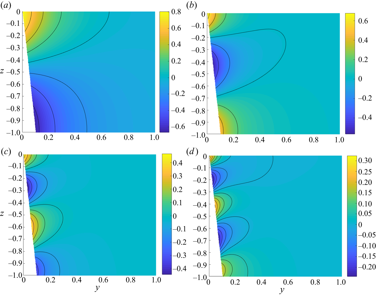
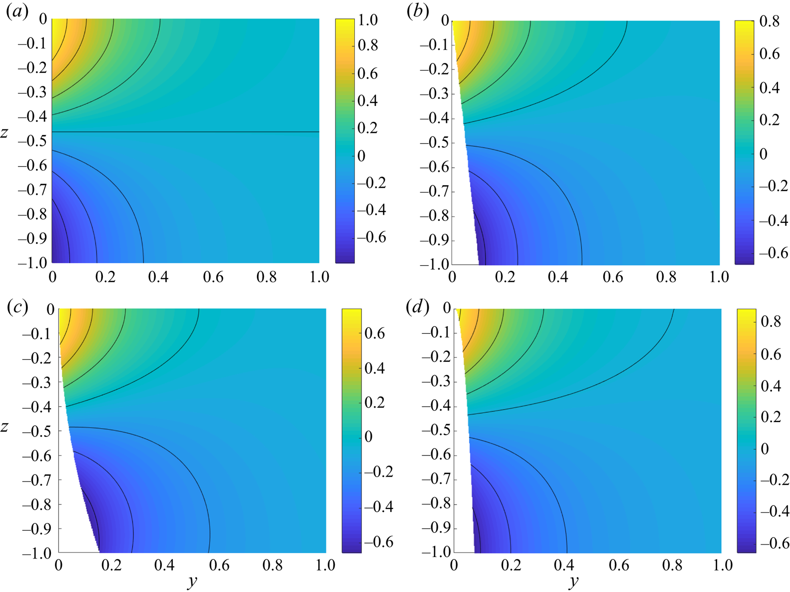
Figure 3 shows  $\textrm {Re}[\phi ^{(n)}]$ for the first four mode numbers and a linear slope
 $\delta (z) = -z$. Near the boundary, disturbances decay approximately with the perpendicular distance from the wall while over larger distances the stratification flattens the phase lines.
Value of  $\textrm {Re}[\phi ^{(n)}]$ for
 $\mathcal {N}^2 = \exp (z)$,
 $D_u = D_b = -({\rm \pi} /2) \sin ({\rm \pi} z)$,
 $\delta = -z$,
 $\epsilon = 0.1$,
 $k = 1$ and
 $Pr = 1$. We show the first four modes
 $n=1,2,3,4$. (a)
 $n= 1$, (b)
 $n= 2$, (c)
 $n= 3$ and (d)
 $n= 4$.
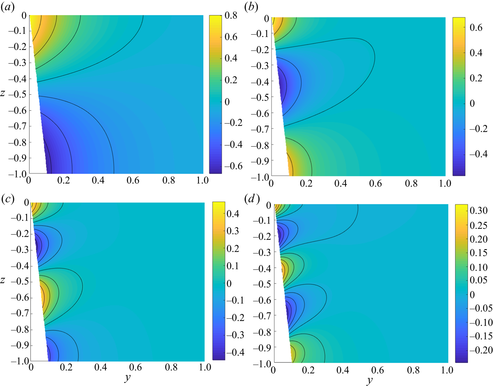
Furthermore, the reduction in magnitude for larger  $n$ suggests that the slope acts to suppress the amplitude of pressure field and hence the along-shore velocity for high mode numbers. We note that an effect of the slope is to induce an
 $O(\epsilon )$ offshore velocity (
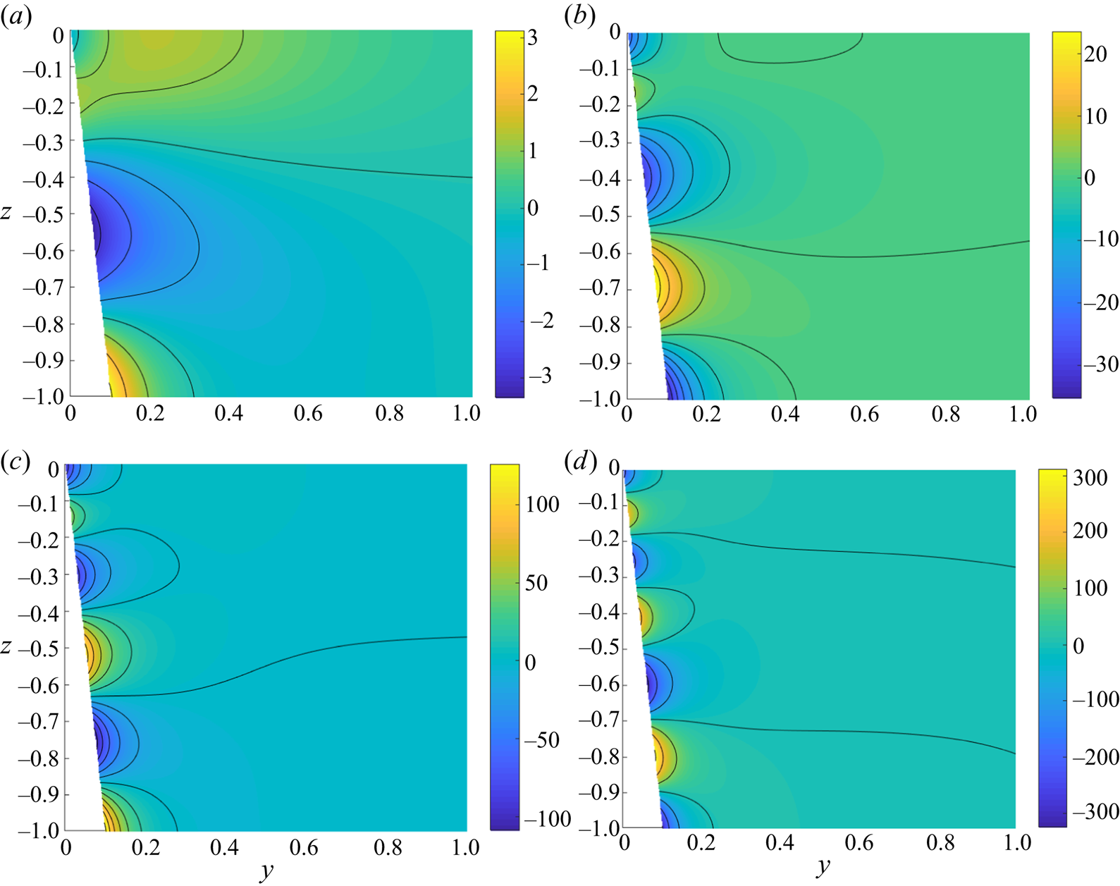
 $v$) which is likely related to the decrease in along-shore velocity. Figure 4 shows
 $\textrm {Im}[\phi ^{(n)}]/\mathcal {E}$ for the same mode number and slope. We can see that vertical mixing induces higher mode number corrections to the
 $n$th mode. Additionally, the large amplitudes for higher
 $n$ suggests that vertical mixing acts more strongly on higher modes. This is consistent with our observations in § 7 that vertical mixing preferentially damps the highest-order modes.
Value of  $\textrm {Im}[\phi ^{(n)}]/\mathcal {E}$ for
 $\mathcal {N}^2 = \exp (z)$,
 $D_u = D_b = -({\rm \pi} /2) \sin ({\rm \pi} z)$,
 $\delta = -z$,
 $\epsilon = 0.1$,
 $k = 1$ and
 $Pr = 1$. We show the first four modes
 $n=1,2,3,4$. (a)
 $n= 1$, (b)
 $n= 2$, (c)
 $n= 3$ and (d)
 $n= 4$.

Figure 5 shows the first mode,  $\textrm {Re}[\phi ^{(1)}]$, for a range of steep slope topographies. A notable feature of the distorted modes is that the zero contour can intersect with the top surface, this can significantly affect the form of the along-shore surface velocity by inducing sign changes along the
 $y$ direction. Note that since
 $\textrm {Im}[\phi ^{(n)}]/\mathcal {E}$ only depends on
 $\delta$ though
 $\lambda$, topographic effects appear only as a depth-dependent horizontal translation. Therefore, since these effects appear predominately in the real part of
 $\phi ^{(n)}$,
 $\textrm {Im}[\phi ^{(1)}]/\mathcal {E}$ is not shown here.
The  $n=1$ mode
 $\textrm {Re}[\phi ^{(1)}]$ for
 $\mathcal {N}^2 = \exp (z)$,
 $D_u = D_b = -({\rm \pi} /2) \sin ({\rm \pi} z)$,
 $\epsilon = 0.1$,
 $k = 1$ and
 $Pr = 1$. We show a range of slope geometries
 $\delta (z) = 0, -z, 3z^2/2, 3\sqrt {|z|}/4$. (a)
 $\delta (z) = 0$, (b)
 $\delta (z) = -z$, (c)
 $\delta (z) = 3z^2/2$ and (d)
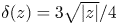 $\delta (z) = 3\sqrt {|z|}/4$.

4.4. The amplitude evolution
Using the dispersion relation
 \begin{equation} \omega^{(n)} = k(U+c_n-\epsilon \gamma_{nn}) - \textrm{i} \epsilon \mathcal{E} \left(\varepsilon_{nn} + \frac{1}{{Pr}}\sigma_{nn}\right), \end{equation}
correct to  $O(\epsilon )$ we can determine an evolution equation for the amplitude,
 $A_n$, as
 \begin{equation} \frac{\partial A_n}{\partial t} + (U+c_n-\epsilon\gamma_{nn}) \frac{\partial A_n}{\partial x} = -{E}\left(\varepsilon_{nn}+\frac{1}{{Pr}}\sigma_{nn}\right)A_n, \end{equation}
where we have substituted  ${E} = \epsilon \,\mathcal {E}$. This equation can be solved as the product of a travelling wave and exponential decay
 \begin{equation} A_n = B_n ( x - (U+c_n-\epsilon\gamma_{nn})t) \exp\left[-{E}\left(\varepsilon_{nn}+\frac{1}{{Pr}}\sigma_{nn}\right)t\right], \end{equation}
for some function  $B_n$ determined by initial conditions. We note that perturbations decay on a time scale of
 \begin{equation} t \sim \frac{1}{{E}(\varepsilon_{nn}+\sigma_{nn}/{Pr})}, \end{equation}
corresponding to a distance of
 \begin{equation} x \sim \frac{U+c_n-\epsilon\gamma_{nn}}{{E}(\varepsilon_{nn}+\sigma_{nn}/{Pr})}. \end{equation}
4.5. The decoupled modes case
One particularly simple example which illustrates some of the effects of vertical mixing is the case of  $\delta = 0$ and
 $D_u\mathcal {N}^2 = D_b\mathcal {N}^2 = 1$. Here, we have
 $\gamma _{mn} = 0$ and
 \begin{equation} \varepsilon_{mn} = \sigma_{mn} = \frac{1}{2c_n^2}\delta_{mn}, \end{equation}
so the vertical modes decouple giving that
 \begin{equation} \phi_{1}^{(n)} = \frac{\textrm{i}\mathcal{E}}{2kc_n^4}\left(1-\frac{1}{{Pr}}\right)y \exp\left[-\frac{y}{c_n}\right]\mathcal{Z}_n(z), \end{equation}
and hence
 \begin{equation} \phi^{(n)} = \phi_0^{(n)} + \epsilon\phi_1^{(n)} + O(\epsilon^2) = \left[ 1 + \frac{i\epsilon\mathcal{E}}{2kc_n^4}\left(1-\frac{1}{{Pr}}\right)y\right] \exp\left[-\frac{y}{c_n}\right]\mathcal{Z}_n(z) + O(\epsilon^2). \end{equation}
We note that, due to the decoupling of the modes, we do not observe the high mode number corrections from mixing effects seen in figure 4. Equation (4.68) can be rewritten as
 \begin{equation} \phi^{(n)} = \exp\left[-\frac{y}{c_n}\left(1-\frac{\textrm{i}{E}}{2kc_n^3} \left[1-\frac{1}{{Pr}}\right]\right)\right]\mathcal{Z}_n(z) + O(\epsilon^2), \end{equation}
with the complex exponential dependence corresponding to decaying offshore oscillations as discussed in Davey et al. (Reference Davey, Hsieh and Wajsowicz1983) and Martinsen & Weber (Reference Martinsen and Weber1981). The full pressure field can be written as
 \begin{align} p &= \sum_{n=0}^\infty \left[\int_{-\infty}^\infty \frac{1}{2{\rm \pi} }\tilde{A}_n(k)\exp\left[-\frac{y}{c_n}\left(1-\frac{\textrm{i}{E}}{2kc_n^3}\left[1-\frac{1}{{Pr}}\right]\right)\right]\mathcal{Z}_n(z) \right. \nonumber\\ &\quad \times \left.\exp\left[ \textrm{i} k\left(x-\left(U+c_n\right)t\right) - \frac{{E}}{2c_n^2}\left(1+\frac{1}{{Pr}}\right)t \right]\, \textrm{d} k \right]+O(\epsilon^2), \end{align}
where we note that all wavenumbers for a given vertical mode number decay at the same rate, given by
 \begin{equation} t \sim \frac{2c_n^2}{{E}}\left(1+\frac{1}{{Pr}}\right)^{-1}. \end{equation}
In the case of  ${Pr} = \infty$ we recover the weak mixing limit of Davey et al. (Reference Davey, Hsieh and Wajsowicz1983) and Martinsen & Weber (Reference Martinsen and Weber1981). Note that it was also shown (Martinsen & Weber Reference Martinsen and Weber1981) that the wave speed is modified by a term proportional to the vertical Ekman number squared, however, in our formulation this effect would be
 $O(\epsilon ^2)$ so is not seen here. For the case of
 ${Pr} = 1$ there are no offshore oscillations and we can write
 \begin{equation} p = \sum_{n=1}^\infty \left[ A_n(x-(U+c_n)t)\exp\left[-\frac{y}{c_n}- \frac{{E}}{c_n^2 } t \right] \mathcal{Z}_n(z) \right] +O(\epsilon^2), \end{equation}
consistent with the observations of Davey et al. (Reference Davey, Hsieh and Wajsowicz1983) that mixing with  ${Pr} = 1$ does not modify the speed or spatial structure of the wave.
5. The nonlinear problem
We now return to the weakly nonlinear problem with  ${Ro} = O(\epsilon )$, corresponding to
 $\mathcal {R} = O(1)$ in (3.12)–(3.14). Since we can no longer invoke linearity, we cannot restrict consideration to normal mode solutions and so instead we expand
 \begin{equation} p = p_0 + \epsilon p_1 + O(\epsilon^2), \end{equation}
and solve directly for  $p_0$ and
 $p_1$. The leading-order system is unchanged from the linear case as
 ${Ro} = \epsilon \mathcal {R} = O(\epsilon )$ so nonlinear effects only appear at
 $O(\epsilon )$ or higher. Therefore we have leading-order solution
 \begin{equation} p_0 = \sum_{n=1}^\infty A_n(x-(U+c_n)t) \exp\left[-\frac{\lambda}{c_n}\right]\mathcal{Z}_n(z). \end{equation}
For simplicity we assume that the leading-order pressure consists of a single mode only,
 \begin{equation} p_0 = p_0^{(n)} = A_n(x-(U+c_n)t) \exp\left[-\frac{\lambda}{c_n}\right]\mathcal{Z}_n(z), \end{equation}
and since we do not have a slowly varying frequency component,  $\omega _1$, in this formulation we instead introduce a slow time scale
 $T = \epsilon t$ and assume that
 $A_n$ varies with
 $T$. Time derivatives can now be expanded using a multiple scale assumption as
 \begin{equation} \frac{\partial }{\partial t} \to \frac{\partial }{\partial t} + \epsilon \frac{\partial }{\partial T}. \end{equation}
From  $p_0^{(n)}$ we can calculate
 \begin{gather} u_0^{(n)} = \frac{1}{c_n}A_n \exp\left[ -\frac{\lambda}{c_n}\right] \mathcal{Z}_n, \end{gather}
 \begin{gather}v_0^{(n)} = 0, \end{gather}
 \begin{gather}w_0^{(n)} = \frac{c_n}{\mathcal{N}^2}A_n' \exp\left[ -\frac{\lambda}{c_n}\right] \mathcal{Z}_n', \end{gather}
 \begin{gather}b_0^{(n)} = A_n \exp\left[ -\frac{\lambda}{c_n}\right] \mathcal{Z}_n'. \end{gather}
Hence, we can calculate the leading-order nonlinear terms as
 \begin{gather} F_{u0} = A_n A_n' \exp\left[ -\frac{2\lambda}{c_n}\right] \left[ \frac{1}{c_n^2}\mathcal{Z}_n^2 + \frac{1}{\mathcal{N}^2} \mathcal{Z}_n'^2 \right], \end{gather}
 \begin{gather}F_{v0} = 0, \end{gather}
 \begin{gather}F_{b0} = A_n A_n' \exp\left[ -\frac{2\lambda}{c_n}\right] \left[ \frac{1}{c_n}\mathcal{Z}_n \mathcal{Z}_n' + \frac{c_n}{\mathcal{N}^2} \mathcal{Z}_n' \mathcal{Z}_n'' \right]. \end{gather}
We note that  $F_v = 0$ everywhere and
 $F_b = 0$ at
 $z= -1,0,$ hence (3.12)–(3.14) reduce to
 \begin{align} &(1+\mathcal{L}_u^2) \left(\frac{\partial }{\partial z}-\epsilon\delta' \frac{\partial }{\partial \lambda}\right)\left[\frac{1}{\mathcal{N}^2}\mathcal{L}_b\left(\frac{\partial p}{\partial z}-\epsilon\delta' \frac{\partial p}{\partial \lambda}\right)\right] + \mathcal{L}_u\left(\frac{\partial ^2}{\partial x^2} + \frac{\partial ^2}{\partial \lambda^2}\right)p \nonumber\\ & \quad = -\epsilon\mathcal{R} \left[ -\frac{\partial F_u}{\partial \lambda} + \mathcal{L}_u \frac{\partial F_u}{\partial x} + (1+\mathcal{L}_u^2) \frac{\partial }{\partial z}\left[\frac{F_b}{\mathcal{N}^2}\right] \right], \end{align}
subject to
 \begin{equation} \frac{\partial p}{\partial z}=\epsilon\delta' \frac{\partial p}{\partial \lambda}\quad \textrm{at} \ z=-1,0, \end{equation}
and
 \begin{equation} \frac{\partial p}{\partial x} - \mathcal{L}_u\frac{\partial p}{\partial \lambda} = -\epsilon(1+\mathcal{L}_u^2)\left[ \frac{\delta'}{\mathcal{N}^2} \mathcal{L}_b \frac{\partial p}{\partial z}\right] - \epsilon\mathcal{R} F_u\quad \textrm{at} \ \lambda = 0, \end{equation}
where
 \begin{equation} \mathcal{L}_u = \left[\frac{\partial }{\partial t} + U \frac{\partial }{\partial x} + \epsilon\frac{\partial }{\partial T} - \epsilon \mathcal{E} \frac{\partial }{\partial z}\left(D_u(z) \frac{\partial }{\partial z}\right)\right], \end{equation}
and
 \begin{equation} \mathcal{L}_b = \left[\frac{\partial }{\partial t} + U \frac{\partial }{\partial x} + \epsilon\frac{\partial }{\partial T} - \frac{\epsilon\mathcal{E}}{{Pr}} \frac{\partial }{\partial z}\left(D_b(z) \frac{\partial }{\partial z}\right)\right]. \end{equation}
We now consider the  $O(\epsilon )$ system to determine the nonlinear evolution of the amplitude
 $A_n$.
5.1. The $O(\epsilon )$ balance

Similarly to the linear case, we can now use leading-order solution to determine the  $O(\epsilon )$ correction. While we will present the governing equations for all vertical modes of this correction term, we will only give the solution for the case where the vertical structure of the correction matches that of the leading-order mode. In this case a secularity condition will allow us to determine the slow evolution of the amplitude,
 $A_n$. The
 $O(\epsilon )$ system is
 \begin{align} &\mathcal{A}_0\left(1+\mathcal{A}_0^2\right)\frac{\partial }{\partial z}\left[\frac{1}{\mathcal{N}^2}\frac{\partial p_1^{(n)}}{\partial z}\right] + \mathcal{A}_0\left(\frac{\partial ^2}{\partial x^2} + \frac{\partial ^2}{\partial \lambda^2}\right)p_1^{(n)} \nonumber\\ &\quad = \mathcal{A}_0\left(1+\mathcal{A}_0^2\right)\left[ \frac{\partial }{\partial z}\left( \frac{\delta'}{\mathcal{N}^2} \right) \frac{\partial p_0^{(n)}}{\partial \lambda}+2\frac{\delta'}{\mathcal{N}^2}\frac{\partial ^2p_0^{(n)}}{\partial z\partial\lambda} \right] + \frac{\mathcal{E}}{{Pr}}\left(1+\mathcal{A}_0^2\right) \frac{\partial }{\partial z}\left[ \frac{1}{\mathcal{N}^2} \mathcal{D}_b \frac{\partial p_0^{(n)}}{\partial z} \right] \nonumber\\ & \qquad +2\mathcal{A}_0^2\left[-\frac{\partial }{\partial T}+\mathcal{E}\mathcal{D}_u\right] \frac{\partial }{\partial z}\left[\frac{1}{\mathcal{N}^2} \frac{\partial p_0^{(n)}}{\partial z} \right] + \mathcal{E}\mathcal{D}_u \left(\frac{\partial ^2}{\partial x^2} + \frac{\partial ^2}{\partial \lambda^2}\right)p_0^{(n)} \nonumber\\ &\qquad -\mathcal{R} \left[ -\frac{\partial F_u}{\partial \lambda} + \mathcal{A}_0 \frac{\partial F_u}{\partial x} + \left(1+\mathcal{A}_0^2\right) \frac{\partial }{\partial z}\left[ \frac{F_b}{\mathcal{N}^2}\right]\right], \end{align}
subject to
 \begin{equation} \frac{\partial p_1^{(n)}}{\partial z} = \delta' \frac{\partial p_0^{(n)}}{\partial \lambda}\quad \textrm{at} \ z = -1,0, \end{equation}
and
 \begin{align} \left[\frac{\partial }{\partial x} - \mathcal{A}_0\frac{\partial }{\partial \lambda}\right]p_1^{(n)} = \left[\frac{\partial }{\partial T}-\mathcal{E}\mathcal{D}_u\right] \frac{\partial p_0^{(n)}}{\partial \lambda} -\frac{\delta'}{\mathcal{N}^2}\mathcal{A}_0\left(1+\mathcal{A}_0^2\right) \frac{\partial p_0^{(n)}}{\partial z} - \mathcal{R} F_u\quad \textrm{at} \ \lambda = 0. \end{align}
Similarly to the linear case, this can be simplified by substituting
 \begin{equation} p_1^{(n)} = q_1^{(n)} + \delta\frac{\partial p_0^{(n)}}{\partial \lambda}, \end{equation}
to get a system for  $q_1^{(n)}$. Given the functional dependence of the forcing we now take
 \begin{equation} q_1^{(n)} = q_1^{(n)}( x - (U+c_n)t, \lambda,z,T), \end{equation}
so
 \begin{equation} \mathcal{A}_0 = -c_n\frac{\partial }{\partial x}, \end{equation}
and expand  $q_1$ as
 \begin{equation} q_1^{(n)} = \sum_{m=0}^\infty q_{1m}^{(n)} \mathcal{Z}_m. \end{equation}
Finally, we substitute for the right-hand side terms in (5.12) to give the following system for  $q_{1m}^{(n)}$
 \begin{align} &\left[\frac{\partial ^2}{\partial \lambda^2}-\frac{1}{c_m^2}-\frac{c_n^2-c_m^2}{c_m^2}\frac{\partial ^2}{\partial x^2} \right]\frac{\partial q_{1m}^{(n)}}{\partial x}\nonumber\\ &\quad\! =\!\left[-\frac{2\delta_{mn}}{c_n}\frac{\partial ^2}{\partial x^2}\frac{\partial A_n}{\partial T}- \frac{2\mathcal{E}\sigma_{mn}}{{Pr}\,c_n^3}\left(1+c_n^2\frac{\partial ^2}{\partial x^2}\right)A_n + \frac{2\mathcal{E}\varepsilon_{mn}}{c_n^3}\left(1-c_n^2\frac{\partial ^2}{\partial x^2}\right)A_n \right]\exp\left[-\frac{\lambda}{c_n}\right]\nonumber\\ & \qquad \!+ \mathcal{R} \left[ \frac{3\alpha_{mn}}{c_n^3}\left[2-c_n^2\frac{\partial ^2}{\partial x^2}\right](A_nA_n') - \frac{3\beta_{mn}}{c_n^3} \left(1+c_n^2\frac{\partial ^2}{\partial x^2}\right)(A_nA_n') \right]\exp\left[-\frac{2\lambda}{c_n}\right], \end{align}
subject to
 \begin{align} &\left[1 + c_n\frac{\partial }{\partial \lambda}\right]\frac{\partial q_{1m}^{(n)}}{\partial x} = -\frac{\delta_{mn}}{c_n}\frac{\partial A_n}{\partial T}-\frac{2\mathcal{E}\varepsilon_{mn}}{c_n}A_n \nonumber\\ &\quad +\frac{\gamma_{mn}}{c_n} \left(1+c_n^2\frac{\partial ^2}{\partial x^2}\right)\frac{\partial A_n}{\partial x} - \frac{3\mathcal{R}\alpha_{mn}}{c_n} (A_n A_n')\quad \textrm{at} \ \lambda = 0, \end{align}
where
 \begin{equation} \alpha_{mn} = \frac{1}{3c_n z_m^2}\int_{-1}^0 \left[ \mathcal{Z}_n^2 + \frac{c_n^2}{\mathcal{N}^2} \mathcal{Z}_n'^2 \right] \mathcal{Z}_m\,\textrm{d} z, \end{equation}
and
 \begin{equation} \beta_{mn} = -\frac{1}{3c_n z_m^2}\int_{-1}^0 \frac{\partial }{\partial z}\left[ \frac{c_n^2}{\mathcal{N}^2}\mathcal{Z}_n \mathcal{Z}_n' + \frac{c_n^4}{\mathcal{N}^4} \mathcal{Z}_n' \mathcal{Z}_n'' \right]\mathcal{Z}_m\,\textrm{d} z, \end{equation}
describe the effects of nonlinearity. We note that  $\varepsilon _{mn}$,
 $\sigma _{mn}$ and
 $\gamma _{mn}$ are the same as defined in § 4.2. This system can be solved for any
 $m$ using Fourier transforms in
 $x$. For simplicity, we consider only the case of
 $m=n$ in order to determine the evolution of the amplitude on the slow time scale
 $T$.
5.1.1. Case $m=n$: the $O(\epsilon )$ correction to the $n$th baroclinic mode


Here, we consider the correction term with the same vertical structure as the leading-order mode, hence  $m=n$. We have
 \begin{align} &\left[\frac{\partial ^2}{\partial \lambda^2}-\frac{1}{c_n^2}\right]\frac{\partial q_{1n}^{(n)}}{\partial x} \nonumber\\ &\quad = \left[-\frac{2}{c_n}\frac{\partial ^2}{\partial x^2}\frac{\partial A_n}{\partial T}- \frac{2\mathcal{E}\sigma_{nn}}{{Pr}\,c_n^3}\left(1+c_n^2\frac{\partial ^2}{\partial x^2}\right)A_n + \frac{2\mathcal{E}\varepsilon_{nn}}{c_n^3}\left(1-c_n^2\frac{\partial ^2}{\partial x^2}\right)A_n \right]\exp\left[-\frac{\lambda}{c_n}\right] \nonumber\\ &\qquad + 3\mathcal{R} \left[ \frac{\alpha_{nn}}{c_n^3}\left[2-c_n^2\frac{\partial ^2}{\partial x^2}\right](A_nA_n') - \frac{\beta_{nn}}{c_n^3} \left(1+c_n^2\frac{\partial ^2}{\partial x^2}\right)(A_nA_n') \right]\exp\left[-\frac{2\lambda}{c_n}\right], \end{align}
subject to
 \begin{align} &\left[1 + c_n\frac{\partial }{\partial \lambda}\right]\frac{\partial q_{1n}^{(n)}}{\partial x} = -\frac{1}{c_n}\frac{\partial A_n}{\partial T}-\frac{2\mathcal{E}\varepsilon_{nn}}{c_n}A_n \nonumber\\ &\quad + \frac{\gamma_{nn}}{c_n} \left(1+c_n^2\frac{\partial ^2}{\partial x^2}\right)\frac{\partial A_n}{\partial x} - \frac{3\mathcal{R}\alpha_{nn}}{c_n} (A_n A_n')\quad \textrm{at} \ \lambda = 0, \end{align}
with solution of the form
 \begin{equation} \frac{\partial q_{1n}^{(n)}}{\partial x} = C_{1n} \lambda \exp\left[-\frac{\lambda}{c_n}\right] +C_{2n} \exp\left[-\frac{2\lambda}{c_n}\right]. \end{equation}
Here,  $C_{1n}$ and
 $C_{2n}$ are both set by (5.23) while (5.24) gives a consistency condition which allows us to determine the slow evolution of
 $A_n$. We have
 \begin{align} C_{1n} &= \frac{\partial ^2}{\partial x^2}\frac{\partial A_n}{\partial T}+ \frac{\mathcal{E}\sigma_{nn}}{{Pr}\,c_n^2}\left(1+c_n^2\frac{\partial ^2}{\partial x^2}\right)A_n - \frac{\mathcal{E}\varepsilon_{nn}}{c_n^2}\left(1-c_n^2\frac{\partial ^2}{\partial x^2}\right)A_n, \end{align}
 \begin{align} C_{2n} &= \mathcal{R} \left[ \frac{\alpha_{nn}}{c_n}\left[2-c_n^2\frac{\partial ^2}{\partial x^2}\right](A_nA_n') - \frac{\beta_{nn}}{c_n} \left(1+c_n^2\frac{\partial ^2}{\partial x^2}\right)(A_nA_n') \right], \end{align}
and
 \begin{equation} c_n C_{1n} - C_{2n} = -\frac{1}{c_n}\frac{\partial A_n}{\partial T}-\frac{2\mathcal{E}\varepsilon_{nn}}{c_n}A_n+ \frac{\gamma_{nn}}{c_n} \left(1+c_n^2\frac{\partial ^2}{\partial x^2}\right)\frac{\partial A_n}{\partial x} - \frac{3\mathcal{R}\alpha_{nn}}{c_n}A_n A_n'. \end{equation}
Substituting for  $C_{1n}$ and
 $C_{2n}$ in (5.28) we have
 \begin{align} \left(1+c_n^2\frac{\partial ^2}{\partial x^2}\right) \left[ \frac{\partial A_n}{\partial T} + \mathcal{E}\left( \varepsilon_{nn}+\frac{1}{{Pr}}\sigma_{nn} \right) A_n +\mathcal{R}(\alpha_{nn}+\beta_{nn})A_nA_n' - \gamma_{nn}A_n' \right] = 0, \end{align}
and cancelling the leading operator gives
 \begin{equation} \frac{\partial A_n}{\partial T} = - \mathcal{E}\left(\varepsilon_{nn}+\frac{1}{{Pr}}\sigma_{nn}\right) A_n -\mathcal{R}(\alpha_{nn}+\beta_{nn})A_nA_n' + \gamma_{nn}A_n', \end{equation}
which describes the slow evolution of  $A_n$. In the case of
 $\mathcal {R} = 0$, this evolution is equivalent to the frequency correction,
 $\omega _1$, in the linear problem as given by (4.49).
5.2. Summary
Similarly to the linear case, our solution for  $p$ is given by
 \begin{equation} p = \left(1-\frac{\epsilon\delta}{c_n}\right) A_n\left(x-(U+c_n)t, T\right) \exp \left[-\frac{\lambda}{c_n}\right] \mathcal{Z}_n(z) + \epsilon \sum_{m=0}^\infty q_{1m}^{(n)}(\lambda) \mathcal{Z}_m(z) + O(\epsilon^2), \end{equation}
where  $q_{1m}^{(n)}$ is given by the solution of (5.19) and (5.20) and we have assumed that
 $p_0$ consists only of a single vertical mode with mode number
 $n$. In the general case, where
 $p_0$ consists of a sum of modes, the solution will be much more complicated due to the appearance of new terms corresponding to the nonlinear interactions between each pair of leading-order modes. Therefore, the general solution will consist of a sum over
 $n$ of (5.31) plus these new interaction terms.
We now recall that the full time evolution is given by the multiple scale expansion
 \begin{equation} \frac{\partial A_n}{\partial t} = \left.\frac{\partial A_n}{\partial t}\right|_T + \epsilon \left.\frac{\partial A_n}{\partial T}\right|_t, \end{equation}
so combine our slow evolution result (5.30) with the leading-order advection to give an equation for the full time evolution of the wave amplitude
 \begin{equation} \frac{\partial A_n}{\partial t} + (U+c_n-\epsilon\gamma_{nn})\frac{\partial A_n}{\partial x} +{Ro}(\alpha_{nn}+\beta_{nn})A_n\frac{\partial A_n}{\partial x}= - {E}\left(\varepsilon_{nn}+\frac{1}{{Pr}}\sigma_{nn}\right) A_n. \end{equation}
This is Hopf's equation with linear friction and in the case of  ${Ro}\, (\alpha _{nn}+\beta _{nn}) = 0$ we recover (4.62) with solutions given by (4.63). We now define
 \begin{gather} U_n = U+c_n-\epsilon\gamma_{nn}, \end{gather}
 \begin{gather}a_n = {Ro}(\alpha_{nn}+\beta_{nn}), \end{gather}
and
 \begin{equation} \kappa_n = {E}\left(\varepsilon_{nn}+\frac{1}{{Pr}}\sigma_{nn}\right), \end{equation}
to write
 \begin{equation} \frac{\partial A_n}{\partial t} + U_n \frac{\partial A_n}{\partial x} + a_n A_n\frac{\partial A_n}{\partial x}= - \kappa_n A_n. \end{equation}
Here,  $U_n$ describes advection with a constant speed,
 $a_n$ describes the effects of nonlinearity and
 $\kappa _n$ describes the damping of the amplitude by vertical mixing.
6. Nonlinear evolution of the amplitude
In §§ 4 and 5 we found that the amplitude of the Kelvin waves, say  $A_n$, satisfies (5.37) with vanishing nonlinear coefficient,
 $a_n$, in the linear case. We now examine this equation in order to understand the effects of vertical mixing on a nonlinearly evolving amplitude; specifically we seek to determine if vertical mixing can act to prevent wave breaking.
6.1. Nonlinear solution
We begin by making the coordinate transformation
 \begin{equation} \tau = \kappa_n t,\quad \eta = x - U_n t,\quad F = \frac{a_n}{\kappa_n} A_n, \end{equation}
so (5.37) becomes
 \begin{equation} \frac{\partial F}{\partial \tau} + F\frac{\partial F}{\partial \eta} = -F, \end{equation}
and we impose initial condition
 \begin{equation} F(\eta,\tau = 0) = F_0(\eta) = \frac{a_n}{\kappa_n}A_n(\eta,t=0). \end{equation}
Motivated by the form of the linear solution, (4.63), we now substitute
 \begin{equation} F = G(\eta,\tau)\, \textrm{e}^{-\tau}, \end{equation}
into (6.2) to obtain
 \begin{equation} \frac{\partial G}{\partial \tau} + \textrm{e}^{-\tau} G \frac{\partial G}{\partial \eta} = 0, \end{equation}
subject to
 \begin{equation} G(\eta,\tau = 0) = F_0(\eta). \end{equation}
This system can be solved using the method of characteristics and the solution for  $G$ is given by
 \begin{equation} G(\eta,\tau) = F_0(r), \end{equation}
where  $r = r(\eta ,\tau )$ is defined implicitly by
 \begin{equation} \eta = r + F_0(r)(1-\textrm{e}^{-\tau}). \end{equation}
Therefore our solution for  $F$ can be written as
 \begin{equation} F(\eta,\tau) = F_0(r(\eta,\tau))\, \textrm{e}^{-\tau}. \end{equation}
We note that nonlinear effects enter through  $r$ and the exponential factor corresponds to the decay of the amplitude due to the effects of vertical mixing. The solution will break if
 $r$ becomes multi-valued for any
 $(\eta ,\tau )$.
6.2. Wave breaking
Here we examine the possibility of wave breaking and determine conditions for when breaking will occur. We proceed by substituting
 \begin{equation} \theta = 1 - \textrm{e}^{-\tau}, \end{equation}
into (6.5) to obtain Burger's equation
 \begin{equation} \frac{\partial G}{\partial \theta} + G \frac{\partial G}{\partial \eta} = 0, \end{equation}
and note that solutions to Burger's equation will always break for a smooth initial profile if there is a region of negative gradient. Assuming that the amplitude vanishes as  $x \to \pm \infty$ we note that all non-zero initial profiles must therefore break in
 $\eta -\theta$ space. Since
 $\tau \to \infty$ corresponds to
 $\theta \to 1$ we concluded that solutions to (6.5) will break at some finite time,
 $\tau ^*$, if solutions to Burger's equation, (6.11), would break for some
 $\theta ^*<1$. It can be shown that solutions to Burger's equation first break at
 \begin{equation} \theta = -\frac{1}{F_0'(r(\eta,\theta))}, \end{equation}
hence there will only be breaking solutions for  $F(\eta ,\tau )$ if
 \begin{equation} -F_0' > 1, \end{equation}
for some  $\eta$. This corresponds to
 $r_\infty (\eta )$ being multi-valued where
 $r_\infty$ the value of
 $r$ when
 $\theta = 1$ (corresponding to
 $\tau = \infty$) and is given implicitly by
 \begin{equation} \eta = r_\infty + F_0(r_\infty). \end{equation}
Substituting for  $F_0$ we have that solutions will break if
 \begin{equation} -\frac{a_n}{\kappa_n} \frac{\partial A_n}{\partial x}(x,0) > 1, \end{equation}
for some  $x$. If
 $r$ does become multi-valued at say
 $(\eta ,\tau ) = (\eta ^*,\tau ^*)$ then our solution will break at
 \begin{equation} (x,t) = (\eta^*+U_n \tau^*/\kappa_n,\tau^*/\kappa_n), \end{equation}
where  $(\eta ^*,\tau ^*)$ depends on the ratio
 $a_n/\kappa _n$ through the initial condition since
 $F_0(\eta ) = a_n A_n(\eta ,0)/\kappa _n$. We note that waves will travel further before breaking for larger
 $U_n$ hence topography can modify the distance travelled by the wave before breaking by modifying the speed,
 $U_n$.
6.3. Summary
Combining our results we have full solution
 \begin{equation} A_n = G( r(x-U_n t, \kappa_n t) )\, \textrm{e}^{-\kappa_n t}, \end{equation}
where
 \begin{equation} \eta = r(\eta,\tau) + \frac{a_n}{\kappa_n} G(r(\eta,\tau))(1-\textrm{e}^{-\tau}), \end{equation}
with wave breaking if
 \begin{equation} \max_x\left[-\frac{a_n}{\kappa_n} \frac{\partial G}{\partial x}\right] > 1. \end{equation}
For a given initial amplitude,  $G$, we can see that wave breaking will occur only if the ratio
 $a_n/\kappa _n$ is sufficiently large. Therefore although vertical mixing acts to suppress wave breaking it cannot prevent breaking if the nonlinearity is strong enough. We note that
 $a_n$ may be negative in which case any breaking will occur of the side of the wave with positive gradient.
In the case of weak mixing we can expand  $\textrm {e}^{-\tau }$ for small
 $\tau$ to get
 \begin{equation} \eta = r(\eta,t) + a_n G(r(\eta,t))(t + O(\kappa_n t^2)), \end{equation}
and
 \begin{equation} A_n = G( r(x-U_n t, t) ) (1 + O(\kappa_n t) ). \end{equation}
Taking  $\kappa _n \to 0$ recovers the solution to Burger's equation and we note that all initial profiles will break in the limit of small
 $\kappa _n$.
For weak nonlinearity we have
 \begin{equation} \eta = r(\eta,\tau) + O(a_n), \end{equation}
hence in the limit of  $a_n \to 0$ we have
 \begin{equation} A_n = G(x-U_n t)\, \textrm{e}^{-\kappa_n t}, \end{equation}
which matches the linear result of (4.63). In this case there are no breaking solutions and our solution is a self-similar travelling wave with exponentially decaying amplitude.
Figure 6 shows solutions for  $A_n$ for a range of values of
 $(a_n,\kappa _n)$ including cases of small
 $a_n$ and small
 $\kappa _n$. Solutions are calculated by numerically solving (6.18) for the characteristic variable
 $r$ and using (6.17) to determine
 $A_n$ from the initial condition
 \begin{equation} G(x) = \exp[ -(x-1)^2 ]. \end{equation}
We note that the characteristics do not form straight lines in  $(x,t)$ space; although they do in
 $(x,\theta )$ space. For this Gaussian initial condition, we expect solutions to break if
 \begin{equation} \frac{a_n}{\kappa_n} > \sqrt{\frac{e}{2}}, \end{equation}
which is consistent with figure 6 in which we observe breaking for  $(a_n,\kappa _n) = (0.2,0.1)$ (b) and
 $(0.2,0.01)$ (c) but not for
 $(a_n,\kappa _n) = (0.1,0.1)$ (a) and
 $(0.01,0.1)$ (d). We say that a numerical solution breaks if the characteristic curves, shown as white lines in figure 6, touch at any point in the domain. The solutions in figure 6 which do not break, panels (a) and (d), both exhibit different behaviour due to a very different ratio between nonlinearity and mixing. In figure 6(a) we have
 $a_n/\kappa _n = 1$ so we expect the solution to initially sharpen before the mixing damps the effects of nonlinearity sufficiently that breaking is avoided. Conversely, in figure 6(d),
 $a_n \ll \kappa _n$ so mixing dominates nonlinearity from the start. There is therefore very little nonlinear evolution and the solution remains self-similar, retaining its initial shape while exponentially decaying in time.
Solution for  $A_n$ (6.17) as a function of
 $(x,t)$ for
 $U_n = 0.5$ and
 $(a_n,\kappa _n) = (0.1,0.1)$ (a),
 $(0.2,0.1)$ (b),
 $(0.2,0.01)$ (c) and
 $(0.01,0.1)$ (d). Characteristic curves are shown as white lines and we take Gaussian initial profile,
 $G(x) = \exp [-(x-1)^2]$. We can see that cases (b) and (c) break while case (a) sharpens towards a smooth profile and case (d) remains approximately self-similar.

7. Applications to baroclinic Kelvin waves
Here we calculate typical values for the coefficients,  $a_n$ and
 $\kappa _n$, in order to determine which effects may be relevant physically. For simplicity we assume that the turbulent mixing acting on momentum and buoyancy is independent of depth, so
 $D_u = D_b = 1$. While this assumption is unrealistic, we note that it gives similar values of the coefficients to more realistic mixing parametrisations and hence is used here for simplicity. If we use
 $\mathcal {N}^2 = 1$ we find that the nonlinear terms are orthogonal to the leading-order solution and so do not affect the amplitude evolution. We therefore conclude that the stratification must vary with depth for any nonlinear effects to be observed and take a simple exponential profile
 \begin{equation} \mathcal{N}^2 = \exp(z), \end{equation}
shown in figure 7(a).
(a) Plot of  $\mathcal {N}^2$ as a function of
 $z$. (b) Plot of the first four vertical modes,
 $\mathcal {Z}_n$, as functions of
 $z$. We normalise the
 $\mathcal {Z}_n$ such that
 $\mathcal {Z}_n(0)=1$.

We can solve for the eigenfunctions,  $\mathcal {Z}_n$, and eigenvalues,
 $c_n^{-2}$, numerically and then calculate the values of the nonlinearity and mixing coefficients using the definitions in §§ 4 and 5. Figure 7(b) shows numerical solutions for the first four eigenfunctions,
 $\mathcal {Z}_n$, as functions of
 $z$, we note that the magnitude of the oscillations is smaller near the bottom of the domain since
 $1/\mathcal {N}^2$ is larger corresponding to stronger damping.
Table 1 shows the values of the wave speed  $c_n$, nonlinearity coefficient
 $\alpha _{nn}+\beta _{nn}$, and mixing coefficients
 $\varepsilon _{nn}$ and
 $\sigma _{nn}$ for the first eight vertical modes. We can see that the nonlinearity coefficient decreases with increasing
 $n$ and has a different sign and magnitude for odd and even
 $n$. Conversely the mixing coefficients increase with increasing
 $n$ and are positive. Therefore nonlinearity has a greater effect on waves with a low vertical mode number and mixing has a greater effect on waves with a high vertical mode number. This is unsurprising as we would expect vertical mixing to act more rapidly on waves with smaller vertical scales and nonlinearity to be stronger when the nonlinear terms are projected onto a mode with less oscillations since less cancellation occurs.
Numerical values of  $c_n$,
 $\alpha _{nn}+\beta _{nn}$,
 $\varepsilon _{nn}$ and
 $\sigma _{nn}$ for the first eight vertical modes with
 $\mathcal{N}^2 = \exp (z)$ and
 $D_u = D_b = 1$. Note that
 $a_n = {Ro} (\alpha _{nn}+\beta _{nn})$ and
 $\kappa _n ={E} (\varepsilon _{nn}+\sigma _{nn}/{Pr})$.

Based on our numerical results from table 1 we assume that the nonlinearity and mixing coefficients have a power law dependence on  $n$. The constant and exponent may be determined by fitting the data to a power law to get
 \begin{equation} a_n = {Ro} (\alpha_{nn}+\beta_{nn}) \sim \begin{cases}0.6\, {Ro}\, n^{-1} & (\textrm{odd } n),\\ -0.08\, {Ro}\, n^{-1} & (\textrm{even } n),\end{cases} \end{equation}
and
 \begin{equation} \kappa_n = {E} (\varepsilon_{nn}+\sigma_{nn}/{Pr}) \sim 5\left(1+\frac{1}{{Pr}}\right) {E}\, n^2. \end{equation}
We note that the coefficients depend on the details of the stratification and mixing terms, however, we expect the qualitative behaviour of the  $n$ dependence to hold in general. Additionally, this scaling result for
 $\kappa _n$ is consistent with the decoupled mode case of Martinsen & Weber (Reference Martinsen and Weber1981); Davey et al. (Reference Davey, Hsieh and Wajsowicz1983) considered in § 4.5. Since both nonlinearity and vertical mixing are important when
 $|a_n| \sim \kappa _n$ we require
 \begin{equation} 0.2\,{Ro}\,n^{-1} \sim 5\left(1+\frac{1}{{Pr}}\right) {E}\, n^2 \implies \frac{{E}}{{Ro}} \sim \frac{0.04}{(1+1/{Pr}) n^3}, \end{equation}
for both effects to be important. Here a coefficient of  $0.2$ is taken for
 $a_n$ as an intermediate between the values for positive and negative
 $n$.
Assuming typical submesoscale quantities – a Rossby radius of deformation  $L_R = NH/f \sim 10^4\,\textrm {m}$, Coriolis parameter
 $f \sim 10^{-4}\,\textrm {s}^{-1}$, velocity scale
 $V \sim 0.1 - 1\, \textrm {ms}^{-1}$ and turbulent viscosity and diffusivity
 $\bar {\nu } \sim \bar {\kappa } \sim 10^{-4}-10^{-3}\, \textrm {m}^2\textrm {s}^{-1}$ – we obtain a typical Rossby number of
 ${Ro} \sim 0.1-1$, typical turbulent Ekman number of
 ${E} \sim 10^{-5}-10^{-4}$ and
 ${Pr} = O(1)$. Using these parameters in (7.4) we can see that both nonlinearity and mixing may be similar in magnitude for the first few baroclinic modes. Conversely, mixing will dominate for modes with large vertical mode number
 $n$ due to the presence of small vertical scales. We note that while
 ${E} \ll {Ro}$ for most physical parameters, the effects of vertical mixing may be similar in magnitude to, or even greater than, those of nonlinearity due to the size of the coefficients in table 1; this justifies the inclusion of both mixing and nonlinearity as
 $O(\epsilon )$ effects. Using (4.65) we can determine the horizontal scale over which vertical mixing damps the amplitude as
 \begin{equation} x \sim \frac{U+c_n-\epsilon\gamma_{nn}}{{E} (\varepsilon_{nn}+\sigma_{nn}/{Pr})} \sim \frac{0.025}{{E} (1+1/{Pr}) n^3}. \end{equation}
Here, we use the scaling  $c_n \sim 0.25\,n^{-1}$ – calculated similarly to the scalings for
 $\varepsilon _{nn}$ and
 $\sigma _{nn}$ – and take
 $U,\gamma _{nn} \approx 0$ by assuming that the along-coast flow and topographic correction to the wave speed are small compared to
 $c_n$. Equivalently we can set
 $U = 0$ by working in the frame of the background flow. Note that this scaling for
 $c_n$ is consistent with the analytic result that
 $c_n = 1/({\rm \pi} n)$ for
 $\mathcal {N}^2 = 1$. Using
 ${E} \sim 10^{-4}-10^{-5}$,
 ${Pr} = O(1)$ and assuming a Rossby radius of deformation on the order of
 $L_R \sim 10^4\ \textrm {m}$ we find that vertical mixing and nonlinearity can have an effect over a dimensional scale of
 $x^* \sim 100\text {--}1000\ \textrm {km}$ for low mode number waves with increasingly small scales for larger
 $n$. Therefore we conclude that vertical mixing and nonlinearity may be important for baroclinic Kelvin waves along coastlines with nonlinear effects relevant only for the first few baroclinic modes and vertical mixing dominant at high mode number.
We note that an important effect of  ${Pr} \neq 1$ is to generate offshore oscillations as seen in § 4.5. However, these offshore oscillations do not affect the horizontal decay scale of the modes or the balance between damping and nonlinearity so we expect the predictions made in (7.4) and (7.5) to be accurate for any value of
 ${Pr}$.
8. Conclusions and discussion
Here we have examined the influence of turbulent mixing and weak nonlinearity on the structure and evolution of baroclinic Kelvin waves propagating along a steeply sloping coastal boundary. We have assumed that the turbulent Ekman number, Rossby number and aspect ratio of the slope are small and used multiple time scale analysis and asymptotic analysis to determine the higher-order correction to the classical Kelvin wave solution. We later found, however, that our solution is valid for order unity Rossby numbers due to the small coefficients multiplying the nonlinear correction terms (see § 7). Our results are therefore relevant to the submesoscale Kelvin waves observed by Dewar et al. (Reference Dewar, Berloff and Hogg2011) and Deremble et al. (Reference Deremble, Johnson and Dewar2017) as well as the more traditional ‘long’ Kelvin waves with an along-shore scale of 100–1000 km (Smith Reference Smith1972; Davey et al. Reference Davey, Hsieh and Wajsowicz1983; Romea & Allen Reference Romea and Allen1984).
In the linear case where finite Rossby number effects are neglected we observe that vertical mixing acts to damp modes by reducing the amplitude exponentially with time and introducing decaying offshore oscillations. This observation is consistent with previous work by Martinsen & Weber (Reference Martinsen and Weber1981), Davey et al. (Reference Davey, Hsieh and Wajsowicz1983) and we recover the same quantitative results in the case of large Prandtl number. Damping occurs at the same rate for all horizontal wave numbers but faster for modes with higher vertical mode number and hence smaller vertical scales.
In our analysis we have neglected the effects of the bottom boundary layer which results from enforcing a no-slip condition on the bottom surface. Romea & Allen (Reference Romea and Allen1984) used a simple Ekman layer parametrisation to study the effects of bottom drag and Ekman pumping to obtain results that are qualitatively similar to ours for vertical mixing. They found that the correction due to boundary layer effects is  $O(\sqrt {\nu _b})$ where
 $\nu _b$ is the value of the turbulent diffusivity evaluated at the bottom boundary. While this correction would appear to be larger than our
 $O(\bar {\nu })$ mixing correction we note that there may be regions away from the boundary where the turbulent diffusivity is enhanced beyond its bottom value by processes such as shear instabilities, double diffusion or internal wave breaking (Large et al. Reference Large, McWilliams and Doney2011). In these cases both internal mixing and bottom drag may play an important role in extracting energy from Kelvin waves.
In the long wave limit of small horizontal wave number  $k$ (and hence small frequency
 $\omega$) our linear solution reduces to the steep-slope model of Romea & Allen (Reference Romea and Allen1984) in the case of no vertical mixing. As demonstrated by Romea & Allen (Reference Romea and Allen1984), the effect of a slope is to modify the along-shore wave speed with either an increase or decrease in speed depending on the sign of the slope curvature. Including vertical mixing, our results are quantitatively similar to the case of a frictional bottom Ekman layer (Romea & Allen Reference Romea and Allen1984) with an exponentially decaying amplitude, a modification of the offshore structure by terms with the same offshore decay scale and the introduction of phase shifts. Since topography can modify the wave speed, we note that it can affect the distance a wave will propagate before being damped by mixing effects.
In the case of superinertial waves, ( $\omega > f$), we observe that topography and vertical mixing may drive offshore propagation where waves with high vertical mode number are generated and propagate into the interior before being damped by mixing. This phenomenon may provide a mechanism for transporting energy from the boundary into the interior ocean and will be examined further in future work.
Romea & Allen (Reference Romea and Allen1984) found that bottom friction can force an barotropic flow even in the case of no surface displacement; in the long wave limit this flow was independent of the offshore direction. We similarly observe that vertical mixing can act to force a barotropic mode, but when no restriction is placed on the size of  $k$, we find that this mode satisfies the Poisson equation in the horizontal plane and hence the mode decays away from the boundary with a scale set by the wavenumber. We note that this horizontal structure is also observed in the strong stratification limit of Johnson (Reference Johnson1991). A sloping boundary can similarly drive a barotropic mode, however, in this case the offshore decay scale matches that of the leading-order mode (Romea & Allen Reference Romea and Allen1984). If a free surface condition were used then the system would admit a barotropic Kelvin wave, while Martinsen & Weber (Reference Martinsen and Weber1981) showed that vertical mixing does not act on barotropic modes due to the lack of vertical structure, the wave would be modified by the addition of the forced mode.
For the weakly nonlinear case where we assume small but finite Rossby number we find that the amplitude of a single mode satisfies a nonlinear advection equation with linear friction resulting from vertical mixing. In the case of no vertical mixing this equation reduces to Hopf's equation and solutions will break similarly to the case of equatorial Kelvin waves studied by Boyd (Reference Boyd1980). For non-zero mixing there is a competition between nonlinearity and mixing with mixing dominating over long time scales. Similarly to the linear case, mixing acts to reduce the maximum amplitude through an exponential decay in time while nonlinearity acts to steepen the wave by creating a velocity difference between the regions of maximum and minimum amplitudes proportional to the difference in amplitudes. If mixing decreases the maximum amplitude sufficiently quickly that the wave does not have time to break before the nonlinear term become small, then the solution will remain smooth. If the nonlinearity is strong enough, however, then solutions can break before the nonlinear term is dominated by the linear friction term. Since a steep slope can modify the speed of the wave we observe that topography may modify the distance travelled by the wave before breaking though the time taken to break remains unchanged.
Since vertical mixing alone is not to enough to prevent breaking in cases of strong nonlinearity, neglected terms such as horizontal mixing or non-hydrostatic dispersion will become important as a breaking event is approached and horizontal scales become small (see appendix A). Note that these effects differ from linear friction in that they preferentially damp small horizontal scales so act to smooth discontinuities arising from wave breaking.
When considering the nonlinear case, we assumed that the leading-order pressure field consists of only a single vertical mode so we neglect the nonlinear interaction between different modes. This nonlinear interaction likely modifies the evolution of the mode amplitudes by removing energy from the leading-order wave and could be studied using simple numerical simulations.
Finally, using a simple stratification profile and typical oceanographic parameters we have estimated the size of the nonlinearity and mixing coefficients. We find that nonlinearity is more significant for modes with low vertical mode number  $n$ while vertical mixing dominates for large
 $n$. Therefore, we conclude that nonlinearity and mixing may both be important for rapidly propagating modes with low
 $n$ hence these modes may dissipate or break over long spatial scales. However, for slowly propagating modes with high
 $n$, vertical mixing will rapidly act to damp out any disturbance over short horizontal scales and the effects of nonlinearity can be neglected.
The coupled model of Deremble et al. (Reference Deremble, Johnson and Dewar2017) uses the formation of submesoscale fronts within the boundary region as a means of dissipating mesoscale energy and injecting vorticity back into the ocean interior, these fronts are formed when the interior flow imposes a wall velocity which exceeds the Kelvin wave speed. Therefore nonlinear wave breaking may provide another mechanism by which sharp buoyancy fronts can form so may provide another mechanism for dissipating boundary energy.
While we have considered an idealised theoretical model, the processes we describe – the dissipation of wave energy by vertical mixing and the generation of small scales by nonlinear wave breaking – may be important for understanding the submesoscale dynamics and energetics of coastal regions. Therefore these processes may play a role in both the parametrisation of sources and sinks of mesoscale energy and the closure of the global energy budget.
Acknowledgements
This work forms part of a joint NERC/NSF project with Professor W. K. Dewar of Florida State University and the authors are indebted to Professor Dewar for providing insightful background material. The work was funded by the UK Natural Environment Research Council under grant number NE/S009922/1. The authors would also like to thank Professor David Marshall and three anonymous reviewers whose constructive comments have greatly improved this manuscript.
Declaration of interests
The authors report no conflict of interest.
Appendix A. Regularisation by dispersion and horizontal diffusion
We have seen that vertical mixing alone is not enough to prevent wave breaking in cases of strong nonlinearity. Here we consider non-hydrostatic dispersion and horizontal diffusion which become important at small scales and act to regularise the shock.
Horizontal diffusion can be included by redefining
 \begin{align} \mathcal{D}_u = \frac{\partial }{\partial z} \left[ D_u \frac{\partial }{\partial z} \right] + \epsilon^4 D_u \left[ \frac{\partial ^2}{\partial x^2} + \frac{\partial ^2}{\partial y^2} \right],\quad \mathcal{D}_b = \frac{\partial }{\partial z} \left[ D_b \frac{\partial }{\partial z} \right] + \epsilon^4 D_b \left[ \frac{\partial ^2}{\partial x^2} + \frac{\partial ^2}{\partial y^2} \right], \end{align}
so this effect appears as  $O(\epsilon ^5)$ terms in (2.1). Dispersion due to non-hydrostatic effects is already included in (2.1) through the
 $O(\epsilon ^4)$ time derivative term on the left-hand side of (2.1c). We will proceed by assuming that dispersion and horizontal diffusion appear at
 $O(\epsilon )$ and include these terms in the
 $O(\epsilon )$ system. This derivation could instead be done rigorously by rescaling
 $x$ and
 $t$ by some powers of epsilon in order to promote these terms to
 $O(\epsilon$), similarly to the classical derivation of the Korteweg–de Vries (KdV) equation for internal waves (Grimshaw Reference Grimshaw1981).
We can repeat our weakly nonlinear analysis from § 5 with dispersion and diffusion by including the term
 \begin{equation} T = -\epsilon^4 (1+\mathcal{L}_u^2 ) \frac{\partial }{\partial z} \left[ \frac{\mathcal{L}_b}{\mathcal{N}^2} \left(\frac{\partial }{\partial t}+U \frac{\partial }{\partial x} \right) w_0 \right], \end{equation}
on the right-hand side of (5.7) and redefining the advection–diffusion operators as
 \begin{equation} \mathcal{L}_u = \left[\frac{\partial }{\partial t} + U \frac{\partial }{\partial x} + \epsilon\frac{\partial }{\partial T} - \epsilon \mathcal{E} \frac{\partial }{\partial z}\left(D_u \frac{\partial }{\partial z}\right) - \epsilon^5 \mathcal{E} D_u \left( \frac{\partial ^2}{\partial x^2} + \frac{\partial ^2}{\partial y^2} \right)\right], \end{equation}
and
 \begin{equation} \mathcal{L}_b = \left[\frac{\partial }{\partial t} + U \frac{\partial }{\partial x} + \epsilon\frac{\partial }{\partial T} - \frac{\epsilon\mathcal{E}}{{Pr}} \frac{\partial }{\partial z}\left(D_b \frac{\partial }{\partial z}\right)- \epsilon^5 \mathcal{E} D_b \left( \frac{\partial ^2}{\partial x^2} + \frac{\partial ^2}{\partial y^2} \right)\right]. \end{equation}
Including these new terms at  $O(\epsilon )$ modifies the consistency condition, (5.30), by adding diffusive and dispersive terms to the slow evolution of
 $A_n$. Our damped Hopf equation for
 $A_n$, (5.33), now becomes as damped KdV–Burgers equation, given by
 \begin{align} &\frac{\partial A_n}{\partial t} + (U+c_n-\epsilon\gamma_{nn})\frac{\partial A_n}{\partial x} +{Ro}\left(\alpha_{nn}+\beta_{nn}\right)A_n\frac{\partial A_n}{\partial x} + \frac{\epsilon^4 c_n^3 \nu_{nn}}{2} \frac{\partial ^3 A_n}{\partial x^3} \nonumber\\ & \quad = - {E}\left(\varepsilon_{nn}+\frac{1}{{Pr}}\sigma_{nn}\right) A_n + \epsilon^4 {E} \left( \varepsilon'_{nn} + \frac{1}{{Pr}}\sigma'_{nn}\right)\left(1+c_n^2 \frac{\partial ^2}{\partial x^2} \right) A_n, \end{align}
where
 \begin{gather} \nu_{mn} = - \frac{c_n^2}{z_m^2} \int_{-1}^0 \frac{\partial }{\partial z} \left[ \frac{1}{\mathcal{N}^4} \frac{\partial \mathcal{Z}_n}{\partial z} \right] \mathcal{Z}_m\, \textrm{d} z, \end{gather}
 \begin{gather}\varepsilon'_{mn} = \frac{1}{2 c_n^2 z_m^2} \int_{-1}^0 D_u \mathcal{Z}_n \mathcal{Z}_m \, \textrm{d} z, \end{gather}
and
 \begin{equation} \sigma'_{mn} = -\frac{1}{2 z_m^2} \int_{-1}^0 \frac{\partial }{\partial z}\left[\frac{D_b}{\mathcal{N}^2} \frac{\partial \mathcal{Z}_n}{\partial z}\right] \mathcal{Z}_m \, \textrm{d} z = \frac{1}{2 z_m^2} \int_{-1}^0 \frac{D_b}{\mathcal{N}^2} \frac{\partial \mathcal{Z}_n}{\partial z} \frac{\partial \mathcal{Z}_m}{\partial z} \, \textrm{d} z. \end{equation}
Note that horizontal mixing adds a new linear friction term which appears to drive exponential growth of the amplitude. This term is due to mixing in the offshore direction and arises due to not enforcing a no-slip boundary condition at  $\lambda = 0$, this leads to a momentum flux from the boundary. Since this term is small compared to the damping from vertical mixing and does not become large as along-shore gradients sharpen, we neglect it.
Defining dispersion coefficient,  $d_n$, and horizontal mixing coefficient,
 $h_n$, as
 \begin{equation} d_n = \frac{\epsilon^4 c_n^3 \nu_{nn}}{2} \quad \textrm{and} \quad h_n = \epsilon^4 c_n^2 {E} \left( \varepsilon'_{nn} + \frac{1}{{Pr}}\sigma'_{nn}\right), \end{equation}
we can write
 \begin{equation} \frac{\partial A_n}{\partial t} + U_n \frac{\partial A_n}{\partial x} + a_n A_n \frac{\partial A_n}{\partial x} + d_n \frac{\partial ^3 A_n}{\partial x^3} = -\kappa_n A_n + h_n \frac{\partial ^2A_n}{\partial x^2}, \end{equation}
where  $U_n$,
 $a_n$ and
 $\kappa _n$ are defined in § 5.2. We note that dispersion and diffusion can both regularise our solutions. Diffusion acts to preferentially damp small scales and smooth out a shock, while dispersion acts to advect small scales away from the breaking region preventing the build up which leads to a discontinuity.
If we assume that  $A_n$ and all derivatives of
 $A_n$ tend to zero as
 $x \to \pm \infty$ we can multiply (A 10) by
 $A_n$ and integrate over the horizontal domain to get
 \begin{equation} \frac{1}{2} \frac{\partial }{\partial t} \int_{-\infty}^\infty A_n^2 \, \textrm{d} x + d_n \int_{-\infty}^\infty A_n \frac{\partial ^3A_n}{\partial x^3} \, \textrm{d} x = -\kappa_n \int_{-\infty}^\infty A_n^2 \, \textrm{d} x + h_n \int_{-\infty}^\infty A_n\frac{\partial ^2A_n}{\partial x^2} \, \textrm{d} x, \end{equation}
where the advection and nonlinear terms have been written as vanishing boundary contributions. Using integration by parts we can now write
 \begin{align} \frac{1}{2} \frac{\partial }{\partial t} \int_{-\infty}^\infty A_n^2 \, \textrm{d} x - \frac{d_n}{2} \int_{-\infty}^\infty \frac{\partial }{\partial x} \left[\frac{\partial A_n}{\partial x}\right]^2\, \textrm{d} x = -\kappa_n \int_{-\infty}^\infty A_n^2 \, \textrm{d} x - h_n \int_{-\infty}^\infty \left[\frac{\partial A_n}{\partial x}\right]^2\, \textrm{d} x, \end{align}
hence, the dispersion term vanishes and we have conservation of total energy for the damped KdV–Burgers equation
 \begin{equation} \frac{1}{2} \frac{\partial }{\partial t} \int_{-\infty}^\infty A_n^2 \, \textrm{d} x = -\kappa_n \int_{-\infty}^\infty A_n^2 \, \textrm{d} x - h_n \int_{-\infty}^\infty \left[\frac{\partial A_n}{\partial x}\right]^2\, \textrm{d} x. \end{equation}
Similarly conservation of total momentum is given by
 \begin{equation} \frac{\partial }{\partial t} \int_{-\infty}^\infty A_n \, \textrm{d} x = -\kappa_n \int_{-\infty}^\infty A_n \, \textrm{d} x. \end{equation}
In the case of  $h_n = 0$ we observe that both the energy and momentum decay exponentially (Cavalcanti et al. Reference Cavalcanti, Domingos Cavalcanti, Faminskii and Natali2012) while for
 $\kappa _n = 0$ the total momentum is conserved and the energy decays. We note that horizontal mixing dissipates more energy in regions of high gradient unlike vertical mixing which occurs at the same rate everywhere.