During the four decades preceding the Great War, Germany was one of the fastest growing economies in Europe. Germany's rise to industrial power has traditionally been ascribed to its dynamic steel, chemical, and electrical engineering corporations.Footnote 1 Moreover, Alfred D. Chandler argued that Germany overtook Britain by leapfrogging ahead of it, employing an economic model closer to the successful model of American managerial capitalism than the supposedly failed model of British personal capitalism.Footnote 2 One important component of Germany's managerial capitalism was the coordination of economic activities via various institutional arrangements. Interlocking directorates, close relationships between banks and industry, and, last but not least, cartels were the coordination mechanisms that were well established in Germany at the turn of the twentieth century. Yet while the relevance of interlocking directorates and close bank-industry relationships has been intensively investigated, the economic impact of cartels has not been fully identified.Footnote 3
During the early twentieth century, nearly 400 cartels controlled about one-quarter of the total industrial and mining output in Germany. Cartels are supposed to have lessened the intensity of competition and to have led to greater steadiness of production and prices.Footnote 4 Moreover, at least some of the cartels might have influenced the allocation of production factors. For example, because of more stable prices and output, cartelized steel firms faced less risk, which in turn induced higher rates of fixed capital investment. Comparatively high capital-labor ratios then resulted into high labor productivity without leading to inefficiencies due to overinvestment.Footnote 5 In addition, it seems that at least some cartels did not earn excess profits. More specifically, Lon LeRoy Peters argues that the mighty Rhenish-Westphalian Coal Syndicate (Rheinisch-Westfälisches Kohlensyndikat, RWKS), one of the longest-standing cartels in the world, aimed to stabilize prices and output and not to achieve excess profits.Footnote 6 This hypothesis is supported by findings of Thomas Bittner, who shows that the formation of the RWKS in 1893 did not lead to excess stock market returns for the participating firms.Footnote 7 The stock market's tepid reaction to the cartel might be a sign that managers of cartelized coal mining companies did not use market power to garner monopoly profits. Possibly, they followed a strategy hypothesized by John R. Hicks, namely that the best monopoly profit is a quiet life for the managers.Footnote 8
If managers actually enjoyed a quiet life, cartelized firms should exhibit lower productive efficiency and Imperial Germany's managerial capitalism would look much less successful than Chandler assumed.Footnote 9 We test this hypothesis by estimating a stochastic frontier model using input and output data for 28 coal mining corporations over the years 1881–1913. It turns out that productive efficiency of coal mining corporations was not significantly affected by cartel membership. Moreover, productive efficiency was significantly higher in firms that paid large bonuses to their board members. This indicates that one pillar of the German economic model—cartelization—did not hamper efficiency, whereas another pillar—the modern managerial corporation—offered mechanisms to overcome potential principal-agent problems between the owners and managers of large coal mining corporations.
Beyond this contribution to the economic history of Imperial Germany, our finding adds to the economics of cartels.Footnote 10 One main conclusion derived from theoretical models is that the incentives of individual firms to cheat undermine the stability of cartels. Indeed, most cartels break up very quickly, with the average cartel lasting only about five years. Nevertheless, some cartels survive for very long periods. The fact that a cartel could survive for long periods of time can be taken as evidence for economic success. Yet the consequences of long-lived cartels and their impact on economic variables like output, prices, profits, and productivity have only been partly identified by empirical research. In particular, the effects of cartels on the productive efficiency of the cartelized firms have been more or less neglected.Footnote 11 Our finding that even one of the longest-lasting cartels in the world did not affect productive efficiency is thus a significant contribution to the empirics of industrial organization.Footnote 12
Our article also sheds light on the relationship between product market competition, financial structure, and managerial incentives, a topic much debated by modern economists. On the one hand, lower product market competition may weaken agents' incentives because principals are worse informed about the agents' actions and the threat of bankruptcy declines with rising market power.Footnote 13 The risk of bankruptcy can also be decreased by decreasing the debt ratio, which in turn further diminished managerial incentives.Footnote 14 On the other hand, declining product-market competition increases the marginal return of managerial effort, and therefore weaker product market competition can induce the manager to work harder.Footnote 15 Moreover, if market shares, output, and prices are fixed by the cartel agreement, the only possible way to increase profits is to lower costs, i.e., to be more efficient. Finally, weak product-market competition can alter the market structure since new firms can enter the market. If these new companies then intensify competition, the marginal return of managerial effort would remain constant.Footnote 16 Which effect predominates is an empirical question, which our results help to answer. We show that the financial structure of corporations and product market competition did not affect productive efficiency, and managerial incentives reduced inefficiency.
THE RHENISH-WESTPHALIAN COAL SYNDICATE
The three decades from the 1880s to World War I constitute the later phase of Germany's industrialization with real net national product increasing by 159 percent between 1880 and 1913 and industrial output by 202 percent.Footnote 17 One important factor behind this rapid growth was coal, the main energy source of the day. In particular, metal production, metal processing, chemicals, mining, and transportation relied on coal as an input factor. Furthermore, coal was an important consumption good, used as heating material in the growing urban centers of Germany.Footnote 18 Coal was basically supplied by four sources. The most important German mining districts were the Ruhr district in the west, the Saar area in the southwest, and Silesia in the east of the empire. Furthermore, coal was imported from Britain via Hamburg, Germany's primary seaport. The most important of these sources was the Ruhr district, whose mines supplied about 48 percent of German coal output in 1880 and about 58 percent in 1913.Footnote 19
The quantitative importance of Ruhr coal mining for the German economy is one reason for focusing on it. Moreover, the industrial organization of coal mining in the Ruhr district differed significantly from the organization in other parts of Germany. In the Ruhr district, mining was almost exclusively performed by Aktiengesellschaften (joint-stock companies) or Gewerkschaften. Footnote 20 In the Saar area, the Prussian state was by far the largest player. In Upper Silesia, the government also had significant shares in output, but in this area, most of the coal fields were privately owned and extracted by east Elbian aristocrats.Footnote 21
Already at the end of the 1870s, collusion had become a prominent phenomenon in the Ruhr district. By coordinating individual behavior, the mining firms sought to eliminate what they thought to be “unhealthy” (ungesunde) competition, and thereby to secure what was called “sufficient” (auskömmliche) prices and profits.Footnote 22 Early efforts were aimed at controlling either output or prices. Moreover, even if more sophisticated coordination techniques were used, they were restricted to local areas and lacked mechanisms to punish defectors. As a result, up to the beginning of the 1890s, all collusive arrangements were ineffective in pursuing their goals, and they therefore eventually failed.Footnote 23
In 1893, 98 firms, representing 87 percent of the coal output from the Ruhr district, joined to form the RWKS, commonly referred to as the most powerful collusive arrangement in Imperial Germany.Footnote 24 Its original treaty was revised twice, first in 1896 and for a second time in 1903. With the latter revision, the vertically integrated iron and steel producers, the foundry mines (Hüttenzechen) of the district, which had abstained from membership up to then, joined the cartel. As a result, coal extraction in the Ruhr district was almost completely cartelized (the market share at the end of 1903 was 98.7 percent).
The RWKS was a price- and quota-setting cartel.Footnote 25 In addition, it managed the sales of its members' production. Every participating firm had to commit itself to sell its entire output to the cartel, which in return was obliged to purchase it. Mines that failed to meet their delivery requirements without a valid excuse were punished with a fine. The prices the RWKS charged its customers varied according to the place where the respective coal was sold. In what was known as the “undisputed area” (unbestrittenes Gebiet), the cartel enjoyed advantages in transportation costs that prohibited outsiders from competing. Here, it fixed its prices annually. Variations were only allowed to account for differences in quality. In contrast, prices in the disputed area (bestrittenes Gebiet) were determined competitively. If they fell short of those in the noncompetitive region, the cartel would compensate for the difference. The compensations (as well as the cartel bureaucracy) were financed by a variable percentage deduction from the monthly revenues that the cartel transferred to its members (Umlage).
Production was regulated by assigning each member a participation figure (Beteiligungsziffer), which was allotted on the basis of members' production levels in either 1891 or 1892. The figures were expressed in tons of coal production, but served as quotas that defined a member's share in total output, since the sum of the individual participation figures represented the maximum production capacity of the cartel. In practice, this maximum was hardly ever realized, because the cartel authorities could reduce total output by applying a common percentage reduction to each member's figure if they judged the production capacity to surpass demand.Footnote 26 Cartel members that exceeded their production allowance were punished with severe fines. Mines, which had to produce below their allowed output due to quality problems or delivery commitments, received subsidies.
Given the duration, the impressive market share, and the seemingly tight organization, it seems reasonable to assume that the RWKS was effective in controlling prices and output. On average, price variations for coal declined after cartel formation.Footnote 27 Yet there were obstacles that might have prevented the cartel from successfully pursuing its cause. First of all, due to the large number of firms, negotiation and monitoring costs were presumably high. Moreover, cost structures were heterogeneous since the geological conditions varied substantially between mines in the north and the south of the Ruhr district. Finally, the industry was growing and the output of cartel outsiders was continuously increasing.Footnote 28
Peters has argued that the long duration of the RWKS reflected the flexibility of its contracts.Footnote 29 In particular, the regulation of output allowed the cartel members to behave individualistically. Their participation figures were not permanently fixed and could be changed in several different ways.Footnote 30 During the period in which the first two contracts were valid (1893–1903), a member firm could automatically increase its participation figure if it sank a new production shaft.Footnote 31 When this shaft was registered, the cartel authorities had almost no means to reject the request for a higher quota. Firms could also request a higher participation figure for already existing shafts, but in contrast the RWKS could refuse such an increase if it judged that the coal market was incapable of dealing with extra production. The takeover of another cartel member was a third way to achieve a higher participation figure (without changing the sum of production allowances).Footnote 32
Between 1893 and 1913, the sum of the individual production allowances rose from 35.4 to 84.1 million tons.Footnote 33 Firms made excessive use of the privilege granted by new shaft: new shafts were sunk and then immediately closed again as soon as the higher quota was assigned; ventilation shafts were converted to extraction shafts; single shafts were equipped with additional extraction facilities and thereby turned into double shafts, which were counted as two shafts.Footnote 34 In effect, the constant changes in the relative and absolute importance among its members must have seriously hampered the ability of the cartel bodies to control output effectively.Footnote 35
Finally, simply looking at the combined market shares of its members overstates the market power of the RWKS. First of all, the cartel sold less than 50 percent of its total output in the undisputed territory; the remaining coal had to be marketed at competitive prices.Footnote 36 Occasionally exports had to be subsidized with revenues from sales in the undisputed territory, as they were sold at below domestic market prices. Moreover, collusion on the demand side or large customers might have restricted the market power of the RWKS. For example, 40 percent of the coal was supplied to the iron and steel industry, which was also more or less cartelized in the time period under investigation. Ten percent of the coal was supplied to railways, which were mainly state owned.Footnote 37 Last but not least, after the second revision of the contract the grip of the cartel on the output of its members began to loosen. From the beginning of the RWKS, the coal used to run operations (Selbstverbrauch) had been excluded from a member's delivery commitments. Up until 1903, these provisions applied to the share of output that was needed to run steam engines and used to produce coke or briquettes. Although the coal involved did not have to be delivered to the cartel, it was still subject to control through the quota regime. But after 1903, the coal for running iron and steel works was also declared to be a part of the Selbstverbrauch and to persuade the vertically integrated firms to join the organization, all this coal for self-use was then exempted from cartel quotas.
DATA SOURCES AND DESCRIPTIVE STATISTICS
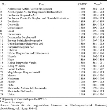
Our sample covers up to 28 mining corporations from the Ruhr district. Data about Gewerkschaften could not be obtained, as they were not obliged to publish the same details about their business operations as joint-stock companies were. The firms in the sample represent between 28 percent (in 1881) and 58 percent (in 1907) of the coal output from this region and 14 percent (in 1881) to 33 percent (in 1907) of the German coal output. Twenty-two of the firms were only engaged in coal mining; the remaining six were vertically integrated foundry mines.
Output and input data were collected from a variety of sources. See Appendices 1 and 2 for a detailed list of firms included in our sample and the exact sources. To estimate a production frontier, output and
DESCRIPTIVE STATISTICS

Sources:
See Appendices 1 and 2.
input measures are required. Our output measure is tons of coal produced during a year; input measures are the number of workers and the value of the fixed assets of a firm, calculated from balance-sheet data.Footnote 38 Accounting figures do not necessarily display the economic value of assets; we therefore apply the perpetual inventory method to compute the capital stock of firms. We use a method proposed by Eric B. Lindenberg and Stephen A. Ross.Footnote 39 Following their approach, the book value of a firm is adjusted for investment, depreciation, price changes, and the technological progress of the current and of preceding periods (for a detailed description, see Appendix 3).
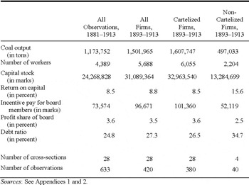
The aggregated input and output figures of the sample clearly show the continuing growth process that characterized the German mining industry between 1881 and 1913 (see Table 1). Coal extraction by the 28 firms increased from 5.7 million tons to 43.9 million tons (682 percent); capital input from 135.5 million marks to 865.3 million marks (538 percent), and labor input from 19,315 workers to 150,890 workers (681 percent). The average coal output of a firm in our sample was nearly 1.2 million tons annually from 1881 to 1913. This output was produced using a capital stock valued at about 24.3 million marks and by employing nearly 4,400 underground workers. During the cartel period (1893–1913), the output, labor input, as well as capital input of cartelized firms were about 2.5 times larger than of non-cartelized firms. Labor productivity was higher in cartelized firms, whereas capital input per worker was higher in non-cartelized firms.Footnote 40 Non-cartelized firms were much more profitable than cartelized firms.
All of the included firms exploited their coal fields with vertically sunk shafts.Footnote 41 Moreover, the technology used to mine the actual coal seams was, with slight variations, identical as well. It was dominated by hand labor; mechanical extraction machines were almost completely absent up to the turn of the century and only slowly accepted afterwards.Footnote 42 In contrast to the similarities in the production technology, there were presumably differences between firms from different parts of the district that could have influenced productivity significantly. Mines situated in the south were faced with thinner and less even seams than those in the north with a lower ratio of coal to stone. These disadvantages were partly offset by the fact that extraction shafts in the northern part of the district had to be deeper in order to reach deposits that were worth exploiting.Footnote 43
The production technology seemed to be similar not only for different firms, but also over time. Labor productivity was nearly constant, and capital intensity was only slightly declining (see Figure 1).Footnote 44 Moreover, a rather simple estimate of the total factor productivity shows that it was nearly constant between 1881 and 1913. Under the simplifying assumptions of constant returns to scale and a labor share of 0.8, the total factor productivity—normalized to 1881 = 100—was 105.4 between 1881 and 1892 and 99.6 between 1893 and 1913.Footnote 45
LABOR PRODUCTIVITY AND CAPITAL INTENSITY FOR A SAMPLE OF RUHR DISTRICT COAL MINING CORPORATIONS, 1881–1913

Besides inputs like capital and labor, theory suggests that market structure, managerial incentives, and capital structure could influence efficiency. We use data about performance-related remuneration paid to the executive and the supervisory boards to measure managerial incentives. The capital structure of each firm is factored into the estimation via the debt ratio, the quotient of debt over total assets. Incentive payments to board members—in marks as well as a share in profits—were significantly higher in cartelized than in non-cartelized firms. This is a first indication that principals in cartelized firms compensated for weaker incentives from product market competition with stronger monetary incentives. On the other hand, the disciplining force of high debt levels was less likely to be used than in non-cartelized firms.
Another important external force influencing managerial effort is competitive pressure from product markets. Product market competition can be measured in a number of ways, for example, by the market share of the largest three corporations or by a Herfindahl index. However, our econometric method uses company-level data. Thus, aggregated proxies of market power are inadequate. Consequently, we measure the influence of the cartel's market power on the productive efficiency of a firm by a dummy variable, taking the value of one if the firm was a member of the RWKS during a given year.
Standard oligopoly theory predicts that a merger of firms in a Cournot oligopoly will not increase the joint profit of the merged firms, but instead increase the profits of the remaining independent market participants.Footnote 46 A similar argument could be at work in the case of the RWKS: the cartel reduced the product market competition not only for the cartel members, but also for the non-cartelized firms. Thus, the productive efficiency of all firms could have declined after cartel formation in 1893. We address this possible effect of the cartel's existence on the productive efficiency of all firms by a dummy variable taking the value of one for all post-1892 observations.
In general, dummy variables might be too imprecise to fully account for the effects of cartelization. Thus, one should also look for a direct disaggregated measure of market power such as firm specific Lerner indices, which would be defined as the ratio of prices to marginal costs. In the case of perfectly competitive markets, prices should equal marginal costs and the price-costs margin should take the value of one. Price-cost margins higher than one would indicate market power. Calculation of marginal costs, however, is quite difficult and often impracticable. Therefore, we use the ratio of prices to average costs, which can be computed for a subsample of our sample (representing about one-third of the total observations). In general, average costs will not equal marginal costs if fixed costs and decreasing returns to scale characterize the production process. The level of our quasi-Lerner indices is thus uninformative. Nevertheless, under the additional assumptions of constant production functions over time, changes in the level of the Lerner index level can serve as an indicator of changes in market power. The ratio of prices to average costs was roughly constant between 1881 and 1913, and it did not shift after the formation of the RWKS in 1893 (see Figure 2). These results cast doubt on the effectiveness of the cartel agreement.
PRICE-AVERAGE COST-MARGIN FOR SUBSAMPLE OF CORPORATIONS, 1881–1913
ECONOMETRIC METHOD
A standard tool for the estimation of productive inefficiency is stochastic frontier analysis.Footnote 47 Basically, a production function y = f(x) describes the relationship between a set of input factors x and output y. For any given x, y must be equal to or less than f(x), so that production always takes place on or below the maximum level of the production function. For an empirical regression model of y = f(x) + ε, the implication is that the error term ε must be negative. In the canonical solution to this problem, any deviation from the production function could arise from two sources: productive inefficiency and idiosyncratic effects that could be either positive or negative.Footnote 48 In addition, firm-specific fixed-effects fi and θi capture fixed firm characteristics, such as different geological settings.Footnote 49
More formally, we estimate production functions described by equations 1a and 1b. Equation 1a describes the very general translog production function, whereas 1b is the standard Cobb-Douglas production function


Equations 1a and 1b are production functions with two inputs, labor Li and capital Ki for firms i = 1, …, 28 and periods t = 1881, …, 1913. Both inputs capital K and labor L, as well as tons of coal output Y, are in logs. Furthermore, we have company- and period-specific random components vi ,t as well as company- and period-specific inefficiency components ui ,t. The term vi ,t captures time- and company-specific idiosyncratic effects, which are normally distributed with a mean of zero. The term ui ,t captures company-specific inefficiencies. These company-specific inefficiencies are censored at zero and can follow different distributions. In the general setting outlined in equations 1a and 1b, the company-specific inefficiencies follow a truncated normal distribution, which is only defined on the positive orthant with a possibly non-zero mode μi; mode μi can in turn be parameterized in terms of company-specific and time-invariant characteristics zi. In equation 2, for example, μmi is explained by the log of the average bonus payments to board members of firm i during the years 1881, …, Ti with observations for firm i.
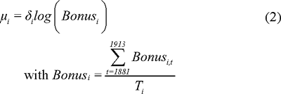
In other specifications of equation 2, we employ the log of the mean dummy variable indicating cartel membership or the ratio of prices to average costs as measures of market power or the log of the mean debt ratio. The effect of one of these variables on productive inefficiency is measured by the size of the coefficient δ. In the baseline specification, we simply assume that μi = 0, in other words, we do not explain productive inefficiency.Footnote 50
Our regressions yield the parameters of the production function. We can therefore identify the relative importance of capital and labor in the production process. The sum of the regression coefficients α 1 and α 2 (or a 1 and a 2) can also be used to test whether the production function has constant returns to scale. Finally, we can use the regression results to calculate productive inefficiency for each firm using a method developed by James Jondrow et al.Footnote 51 Moreover, the aggregate inefficiency for the whole population of firms can be calculated as the mean of company-specific inefficiencies.
RESULTS
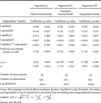
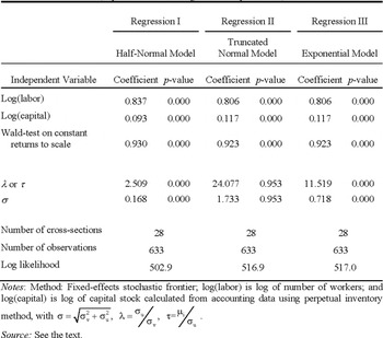
Table 2 shows the results using the translog production function (1a), whereas Table 3 shows the results using the more restrictive Cobb-Douglas production function (1b). Both production functions are estimated using three different specifications regarding the distributions of the firm-specific inefficiency term. The baseline specification is a fixed-effects model with the additional assumption that the firm-specific inefficiencies follow a half-normal distribution with mode 0. In addition, we check the distributional assumption for the inefficiency term by comparing it with models using a truncated normal or an exponential distribution for the inefficiency term. The estimates are quite similar for all three models and we finally opt for a half-normal model, since this allows the parameterization of the inefficiency distribution. We estimate a translog production function using the specification proposed by Vittorio Corbo and Patricio Meller as well as William H. Greene.Footnote 52 The additional parameters in the translog model are insignificant and we therefore turn to the simpler Cobb-Douglas production function.Footnote 53 The decisive difference between the translog
BASELINE REGRESSION RESULTS I: TRANSLOG PRODUCTION FUNCTION: (dependent variable: log of coal output in tons)

Notes:
The estimates are fixed effects stochastic frontier; log(labor) is log of number of workers; and log(capital) is log of capital stock calculated from accounting data using perpetual inventory method, with  .
Source:
See the text.
production function and the Cobb-Douglas production function is that the former does not restrict the values of the elasticity of substitution and it does not assume strong separability among input factors.
The parameter values of the production function displayed in Tables 2 and 3 indicate that coal mining in the late nineteenth-and early twentieth-century Ruhr district was labor intensive, with slightly decreasing economies of scale: the sum of the coefficients for labor (0.837) and capital (0.093) takes a value close to but significantly below one (see Table 3, regression I). In part, this result concurs with the literature on coal mining in the Ruhr district. The great importance of the production factor labor is a common theme in studies on mining in
BASELINE REGRESSION RESULTS II: COBB-DOUGLAS PRODUCTION FUNCTION (dependent variable: log of coal output in tons)

Notes:
Method: Fixed-effects stochastic frontier; log(labor) is log of number of workers; and log(capital) is log of capital stock calculated from accounting data using perpetual inventory method, with  .
Source:
See the text.
the Ruhr district. Reinhard Effertz and Ernst Jüngst find that Labor costs constituted roughly 60 percent of the total costs per ton of coal in the Ruhr district.Footnote 54 Moreover, Carl-Ludwig Holtfrerich's estimates of the shares of capital and Labor in net value added emphasize the great importance of the latter factor.Footnote 55
Our finding of decreasing returns to scale stands in contrast to the dominant view in contemporary studies. Most scholars commonly note that fixed costs in coal mining were substantial and that, in general, increases in output were accompanied by decreasing average costs and thus increasing returns to scale.Footnote 56 However, marginal costs are not considered, because almost all of the contemporary writers have been influenced by the non-marginalistic German historical school of economics. In the only available modern study, Holtfrerich, argues for constant returns to scale.Footnote 57 He notes that the introduction of vertically sunk extraction shafts meant access to a practically infinite number of equally profitable coal deposits. But at the same time having to exploit deeper seated coal worked in the opposite direction, and the two effects cancelled out one another. The underground transportation distance for the extracted coal increased, but the deeper seated coal seams were generally thicker and flatter and more evenly stratified than those closer to the surface.Footnote 58
Our estimates offer no support for the hypothesis of increasing returns to scale, but might be compatible with Holtfrerich's view of constant returns to scale, since our estimate of economies of scale of 0.93 is close to one. However, there are good reasons for believing that Holtfrerich is too optimistic about the positive effects of vertically sunk shafts and thus, for defending our finding of slightly decreasing returns to scale. Without a doubt, vertical shafts did dramatically increase the number of accessible coal deposits. Nonetheless, the stratification of coal seams was still uncertain even for those near existing production facilities. In addition, Holtfrerich omits increases in output achieved by expanding horizontally, where the rewards were often less likely. Rising production had other drawbacks too, no matter what the direction. It rose the distance the coal had to be transported underground. It also lengthened the time workers had to spend getting to the actual extraction points.Footnote 59 Surveillance of workers became increasingly difficult and costly. The same was true for preparing, maintaining, and securing the coal seams and for those of dehydration and ventilation. Although innovative extraction methods, such as the mechanization of transportation and the extraction might compensate, they were in their infancy in the 1890s and much was still at an experimental stage. Furthermore, partial innovations at one stage of the production process had negative repercussions on other links in the chain.Footnote 60 In any event, until 1903 the cartel contract created an incentive to add new shafts in order to get a higher quota. Therefore, the size and distribution of investments was influenced by the design of the cartel contract, which could induce inefficiencies.
Of greater interest for our main research question are the results for the inefficiency parameter. The parameters of the production function estimated by our baseline regression using the Cobb-Douglas production function and the assumption of a half-normally distributed error term lead to an estimation of the mean inefficiency of Ruhr coal mining corporations of about 11.7 percent.Footnote 61
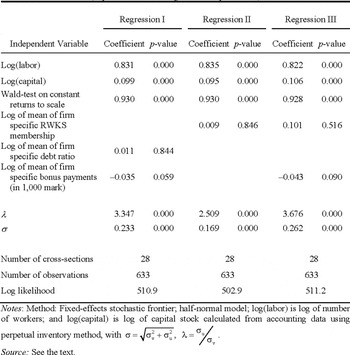
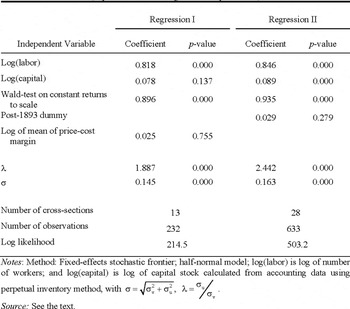
To deepen the analysis, we test whether certain variables—for example, proxies for product market competition or the quality of corporate governance-influenced productive efficiency. Table 4 displays the results of equations 1b and 2 if we allow for a heterogeneous mean μi, which would be affected by firm characteristics such as cartel membership.
It turns out that company-specific inefficiency cannot be explained using cartel membership (Table 4, regression II). The coefficient is statistically insignificant. Furthermore, the results presented in Table 5, regression I, demonstrate that the price-cost margin—which was calculated for a subsample of the total observations available—is also statistically insignificant. And regression II in Table 5 shows that the post-1893 dummy variable—which was intended to pick up possible negative effects of cartel formation on all firms in the sample—is statistically insignificant as well.
Therefore, we take an intermediate position on the impact of cartels on productive efficiency. On the basis of the views of contemporaries, Wilfried Feldenkirchen and Ulrich Wengenroth hypothesize that cartels hampered cost efficiency.Footnote 62 Toni Pierenkemper argues, however, that cartel members had an incentive to reduce costs, since output prices were fixed.Footnote 63 Therefore, cartels should have improved cost efficiency. Our results by contrast demonstrate that cartel formation did not affect the productive efficiency of coal mines.
What about corporate governance? Did it affect efficiency? We can test whether efficiency is influenced by performance-related managerial compensation or differences in the financial structure of the corporations. It turns out that the financial structure of corporations is insignificant in explaining productive efficiency (Table 4, regression I).
EXPLAINING PRODUCTIVE EFFICIENCY: (dependent variable: log of coal output in tons)

Notes:
Method: Fixed-effects stochastic frontier; half-normal model; log(labor) is log of number of workers; and log(capital) is log of capital stock calculated from accounting data using perpetual inventory method, with 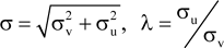 .
Source:
See the text.
But productive inefficiency does happen to be affected by bonus payments to board members: the coefficient is economically substantial and statistically significant at the 10 percent level (Table 4, regressions I and III).Footnote 64 At first glance, the coefficient measuring the efficiency gains of managerial compensation seems to be quite small: an increase of bonus payments to the board by 1 percent only reduces technical inefficiency by about 0.0035 percent. Yet, the monetary equivalent of
EXPLAINING PRODUCTIVE EFFICIENCY: STABILITY TESTS: (dependent variable: log of coal output in tons)

Notes:
Method: Fixed-effects stochastic frontier; half-normal model; log(labor) is log of number of workers; and log(capital) is log of capital stock calculated from accounting data using perpetual inventory method, with 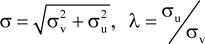 .
Source:
See the text.
technical inefficiency is larger than the value of bonus payments. On average, about 73,000 marks were paid out as a bonus to the board. Thus, an increase of bonus payments of 1 percent amount to about 730 marks. Average costs for a firm were about 193.7 million marks.Footnote 65 The mean inefficiency of a firm is about 11.7 percent, or 22.66 million marks, a 0.0035 percent reduction of technical inefficiency would therefore be about 790 marks. The cost reductions are therefore slightly higher than the additional bonuses paid, which suggest that the bonuses gave managers an incentive to generate higher profits via reduced costs. Such performance-related managerial compensation was much higher in cartelized firms. After cartel formation in 1893, the board of a non-cartelized company received only 2.5 percent of profits as a bonus, whereas the board of a cartelized firm received 3.6 percent.
CONCLUSION
The German Empire is commonly believed to be a nation of cartels. There is some truth in this view, for several hundred cartels existed in pre-World War I Germany and from at least 1897 onwards, cartel agreements were judicially enforceable. But the economic consequences of cartels and their impact on German industrialization have not been explored fully.
Standard theory suggests that cartels should lead to excess profits for cartelized firms. The redistribution of the consumer surplus to producers and the aggregate decline in output should induce social losses. In addition, in a world with asymmetric information between owners of a cartelized mining corporation and managers, the managers have to be motivated by incentives. Otherwise, they could use market power to enjoy a quiet life, instead of the tougher existence of profit-maximizing agents. If so, reduced product market competition could lead to reduced efficiency.
Recent research leads to no clear conclusion either for cartels in general or the RWKS in particular. First, Wengenroth and Feldenkirchen hypothesized that cartelized firms lost flexibility and that they therefore hampered the growth of total factor productivity and static cost efficiency.Footnote 66 Second, Bittner showed that the formation of the RWKS left no mark on stock market returns.Footnote 67 This supports a hypothesis of Karl Erich Born, who argued that the RWKS was unimportant for the development of coal mining in the Ruhr area.Footnote 68 But, Pierenkemper hypothesized that the cartel was in fact successful since it stabilized coal prices and led to higher revenues for the cartelized companies. Moreover, since the price was fixed by the RWKS, the only mechanism available to managers to increase firm profits was cost reduction. Therefore, in his view, the cartel boosted efficiency.Footnote 69
The findings of our article mostly agree with the intermediate position taken by Bittner and Born: the RWKS did not have a measurable effect on the technical efficiency of the cartelized firms. Yet we can also partly support Pierenkemper's claim that cost reduction was a successful strategy, at least if managers of the firms shared increased firm profits. Still, even the supposedly most important cartel in Imperial Germany did not have a measurable impact on the technical efficiency of cartelized firms. The impact of cartels on German industrialization might be much less pronounced than classical accounts suggest.
Appendix 1: Data Sources
Average Costs in Mark
Deutsche Ökonomist, 1881–1889; and Jahrbuch 2–14.
Average Revenues in Mark
Deutsche Ökonomist, 1881–1889; and Jahrbuch 2–14.
Coal Output in Tons
Germany. State Archive. Münster, Inventory Oberbergamt Dortmund (No. 88–101); Huske, Steinkohlenzechen; Jahrbuch 2–14; and Zeitschrift, 30–41.
Labor Input
Germany. State Archive. Münster, Inventory Oberbergamt Dortmund (No. 88–101); Huske, Steinkohlenzechen; and Jahrbuch 2–14.
Capital Input in Marks
Feldenkirchen. Die Eisen- und Stahlindustrie des Ruhrgebiets, 1879–1914.
Saling's Börsen-Jahrbuch 5–38.
Appendix 2: Sample of Mining Corporations
MINING CORPORATIONS INCLUDED IN OUR SAMPLE

a Beginning of membership in the RWKS.
b Years in the sample.
Source:
Verein für die bergbaulichen Interessen im Oberbergamtsbezirk Dortmund, Entwicklung, vol. 11, pp. 304–42.
Appendix 3: Calculation of Capital Stock atReplacement Costs
Following Lindenberg and Ross, the replacement cost (RC) of a firm at time t is the sum of three summands: the total assets of the firm at time t (TAt), the difference between the firm's net plant at replacement cost in period t and the historic value of its net plant in the same period (RNPt– HNPt), and the difference between the firm's inventories at replacement cost and the historic value of its inventories (RINVt – HINVt).Footnote 70
The inventories summand drops out, because contemporaries used to price their inventories at recent prices so that a firm's inventories at replacement cost are equal to the historic value of its inventories (RINVt = HINVt,).Footnote 71 The amount of total assets and the net plant at historical value are taken directly from balance sheets. The net plant at replacement costs is calculated by a recursive estimation procedure that accounts for investment, depreciation, price changes, and technical progress:

φ: Change of capital goods price index
δ: Depreciation rate
θ: Rate of technical progress
I: Investment
The capital goods price index is approximated by Walther G. Hoffmann's machine price index; the rate of technical progress by the residual of the growth accounting exercise of the industrial sector by Carsten Burhop and Guntram B. Wolff.Footnote 72 The depreciation rate was calculated by dividing the depreciation in period t by the historical net plant in the preceding period; investment by subtracting the historical net plant in period t–1 from the historical net plant of the subsequent period and adding the depreciation of period t.
 with Φ (Ф) denoting the distribution function (cumulative distribution function) of the normal distribution.