

I. INTRODUCTION
Polycrystalline materials are solids (e.g., powders, compact bulk materials, ceramics, ionic crystals, metals) deviating from a perfectly ordered structure to form small crystalline domains, which are all contained into grains or particles. The grain size may range from a few to tens of microns. A special class of polycrystalline materials features grain size less than 100 nm and a high density (1019 cm−3) of grain boundaries; this class is called nanocrystalline materials (Gleiter, Reference Gleiter2000). Thin-films (less than 1 µm in thickness) can be classified as epitaxial (single crystal), polycrystalline, or amorphous materials depending on homogeneity in crystalline domains. Catalytic converters, self-cleaning surfaces, magnetic nanostructures, supra-hard composites, among others, are great examples of polycrystalline materials in technological applications (Suryanarayana, Reference Suryanarayana1995).
In the study of polycrystalline materials, a reliable technique for specimen microstructural characterization is transmission electron microscopy (TEM) and high-resolution TEM (Kril and Birringer, Reference Kril and Birringer1998). However, it may become demanding to carry out several evaluations for a series of specimens prepared under different experimental conditions as well as subsequent heat treatments, plastic deformations, doping, sintering, etc. In addition, the information obtained using TEM is local and may not represent the average properties. X-ray diffraction (XRD) technique is a suitable alternative because it usually examines 103–105 larger sample volume than that studied by TEM. Therefore, XRD can offer the advantages of being fast in obtaining a truly statistically averaged information of the specimen, easy preparation of the sample, non-destructive method, and low-cost of maintenance (Snyder et al., Reference Snyder, Fiala and Bunge1999). XRD is also a very valuable tool in undergraduate programs for developing interests in analytical methods, instrumentation, and routine code development (Butera and Waldeck, Reference Butera and Waldeck1997; Pope, Reference Pope1997; Jenkins, Reference Jenkins2001; Ryan, Reference Ryan2001; Stojilovic, Reference Stojilovic2018).
XRD has become a standard technique in many laboratories; it is employed mainly for qualitative analysis and phase identification through a comparison between experimental data and files of reference patterns. To this comparison, the overall methodology for checking single-phase data files is the Rietveld method, in which structural parameters and other instrument effects are refined to match measured data. A second class of analysis is concerned with a structure determination by powder diffractometry (SDPD) for indexed powder patterns. This task is commonly explored through trial-and-error, dichotomy and Monte Carlo approaches. While several programs have appeared on the market to carry on both Rietveld and SDPD routines, there is a third group of methods less spread into the powder diffraction community. This is the group of methods focused on the study of the microstructure properties, namely, crystallite size, size distribution, stacking faults, twin boundaries, dislocations, chemical heterogeneities, vacancies, surface relaxation. Therefore, it would seem that activities for determining particular microstructure parameters from XRD line profiles are often missing in undergraduate programs. So far, the Scherrer equation is traditionally used to approach the crystallite size, which in fact is frequently overestimated, as it does not take into account the presence of sample micro-strain. The procedure of the evaluation of the peak profiles for microstructure analysis is referred to as X-Ray line profile analysis, XLPA (Gubicza, Reference Gubicza2014). XLPA methods are suitable to introduce anisotropic effects from fundamental approaches, and thus evaluate X-ray peak broadening as a correlation between crystallite size and lattice strain. Comparing with Rietveld, XLPA methods determine parameters by fitting theoretical functions on the line profiles (i.e., not necessarily a reference pattern). In this study, ready-to-use coding routines incorporate methodologies of line-broadening analysis to evaluate coherent diffraction domain sizes, size distribution, and lattice microstrain. The objective is to present a set of functions introducing specific methods for handling XRD current problems in the processing X-ray line profiles of experimental data. The bases for the methods to be discussed have been reported previously, and today constitute well-established data processing routines and in state-steady level. In a first approach, the set of routines process XRD data from grains (NaCl), and epitaxial (Si) film and thin-films (Au sputtered from radiofrequency). Undergraduate students of chemistry, physics, and nanotechnology programs can promptly learn how to apply a set of functions creating their own custom scripts to improve skills in the microstructural characterization of polycrystalline materials through of XLPA.
II. IMPLEMENTATION
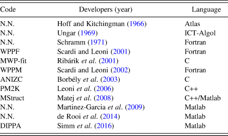
Several routines and computer programs to carry out the analysis for powder diffraction have been published elsewhere (Cranswick, Reference Cranswick, Dinnebier and Billinge2008). A short list of computational contributions to XLPA is described in Table I.
Computational routines developed for XLPA.

In this study, we show a set of routines written in GNU-Octave (v4.2.1) programing language to carry out the pretreatment of XRD data and further study of a microstructure. The set is divided into routines according to the procedures described below. GNU-Octave is chosen for the organization, storage, and analysis of data because this programing language has the capacity to import data from a variety of sources (*.xy, *.dat, *.txt), store the data in arbitrarily data structures (i.e. it can handle easily, compactly, and quickly both vector and matrixes), manipulate such data using built-in and user-defined functions. All output data can be tabulated, and figures can be plotted in the same GUI platform.
A. Background
XRD background arises from a number of sources, including, fluorescent radiation, and incoherent scattering from the specimen, diffraction of the continuous spectrum, collimator, air, etc. The accurate determination of the diffraction peak properties (e.g., height, integrated intensity, integral breadth, centroid, variance, fourth moment, and the Fourier coefficients of the line profile) depends to various extents on an estimation of the background (Mitra and Misra, Reference Mitra and Misra1966). For instance, XLPA is more repeatable if the background has been previously eliminated from the data. The criterion for accepting a peak representing a true X-ray diffraction line would require the peak to be higher than 3–5 standard deviations above background. Two basic algorithms to estimate the background are employed in common programs. The first method uses a predetermined background model and simply adjusts an additive constant. At first, a background intensity is just being user-selected representing a constant count level defined to the entire range of the diffractogram. Anything upper would be considered as a peak including those noise points that surpass the level. Alternatively, the background can be represented through selected points that will be used to model a much more complex function. The intensities of the first and last points (about 100 points) can be selected for drawing a straight line (i.e., the background) through the averaged values. Thus, the background intensity at a point 2θ ican be calculated easily as shown in Eq. (1):
 $$bkgl_i = \left( {\displaystyle{{z-a} \over {2\theta_N-2\theta_1}}} \right)\; 2\theta _i + \displaystyle{{a(2\theta _N)-z(2\theta _1)} \over {2\theta _N-2\theta _1}}$$
where  $z = 1/N \sum \nolimits I(2\theta _i)$ and
 $a = 1/N \sum \nolimits I(2\theta _{N-i})$ are the averaged last and first N points selected.
The second method, which is referred to in this paragraph, uses polynomial approaches. Typically, the background is a collection of points that can be represented by a smoothing curve using polynomials. The first approximation is the method called cubic splines, which consists of construction of curves through piecewise cubic polynomials (i.e., functions numerically well behaved that support inflections). To this, pairs of control points represent short segments of the curve. The solution of coefficients requires conditions of continuity at the joints, slope, and curvature constrain, and limits at the borders to represent a set of linear equation and its solution  ${\bf a} = {\bf M}^{-1}{\bi \;} {\bf y}$, where the vector a contains the corresponding coefficients polynomials.
In order to have local shape control, Hermite cubic splines are employed when parametrizing over tight portions of curves. To this is required slopes in parametric form at each control point. The control points are obtained from raw data for which two-theta and intensity (y 0) values are arranged as vectors. Ideally, these pairs should be taken automatically, i.e., without the user having to select segments of the pattern. The first step obtains the indexes for all points y 0 that are located at a certain background level. The resulting polynomial background coefficients are saved in the directory where the raw data is located allowing to judge the fit and adjust their model or starting parameters accordingly.
B. Profile smoothing
To reduce random noise for a series of counts, the most generalized method in the literature is the Savitzky and Golay smoothing method (Savitzky and Golay, Reference Savitzky and Golay1964). This filter was initially used for spectral lines in noisy spectrometric data, but promptly was adopted in other physical processes in which the enhancement of signal-to-noise ratios is also relevant. The original algorithm has been modified to get better local estimates of the expected values (Luo et al., Reference Luo, Ying and Bai2005; de Rooi et al., Reference de Rooi, van der Pers, Hendrikx, Delhez, Böttgerb and Eilersa2014).
Considering a successive subset of 2m + 1 points that are going to be fitted by a smooth series μ, represented as a polynomial of degree k in j (with k ≤ 2m) and with the same length of the selected points, then such a series μ and its nth derivative can be represented as Eqs (2) and (3):
 $$\mu _j = \sum \limits_{k = 0}^{k = n} b_{n,k}j^k = b_{n,0} + b_{n,1}j^1 + b_{n,2}j^2 + \cdots + b_{n,n}j^n$$
 $$\displaystyle{{d^n\mu _j} \over {dj^n}} = n!b_{n,n}$$
The coefficients b n,n are to be selected in such a way that when each j-point data (abscissa) is substituted into μ j, then the sum of the squares of the differences between the computed values (μ j) and the observed values (y j) are required to be a minimum over the interval being considered. Thus, the least-squares criterion is used to measure the fit,
 $$\displaystyle{\partial \over {\partial b_{n,k}}}\left[ {\mathop \sum \limits_{\,j = -m}^{\,j = m} {\lpar {\mu_j- y_j} \rpar }^2} \right] = 0\; $$
If a minimization is considered with respect to the rth differentiation,
 $$2\mathop \sum \limits_{\,j = -m}^{\,j = m} \left[ {\left( {\mathop \sum \limits_{k = 0}^{k = n} b_{n,k}j^k} \right)-y_j} \right]j^r = 0$$
The running least-squares polynomial fitting can be automatically performed by convolving the entire input data with a digital filter. The running equation follows as Eq. (6),
 $$\mathop \sum \limits_{k = 0}^{k = n} b_{n,k}S_{r + k} = F_k$$
where 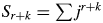 $S_{r + k} = \sum \nolimits j^{r + k}$ and
 $F_k = \mathop \sum \nolimits j^ky_j$. In principle, the convolution coefficients are obtained for all data points, all polynomial degrees and all differentiation orders.
IndexCub uses a routine that performs smoothing with an algorithm based on the method published by de Rooi et al. (Reference de Rooi, van der Pers, Hendrikx, Delhez, Böttgerb and Eilersa2014) showing a penalized likelihood smoothing approach. The line-profile is mathematically smoothed by a least-squares fit of a series (i.e. polynomial) of points that does not deviate too much of the original data and without loss of resolution. Such a strategy provides the possibility of using nth-order decomposition on the experimental data. Taking advantage of a simple averaging of a large number of counts, at first the noise is reduced as the square root of the number of “points”. Then it can sometimes be useful to replace each data point by some kind of local average of surrounding data points.
C. K α 2 radiation removal
In comparison with single crystals, which show narrow diffraction peaks, polycrystalline specimens diffraction patterns show peaks not only broadened but also containing doublets. The origin of these doublets comes from X-ray tube sources, which give radiation beyond the simple Kα emission required for diffraction measurements. This additional radiation includes other emission lines from the anode, including a strong Kβ emission, and emission lines from tube impurities such as tungsten, arising from the tube cathode. While physical filtering or monochromators are used to reduce Kβ radiation, computational routines subtract Kα 2 radiation.
A classical routine for stripping Kα 2 radiation is based on the Rachinger correction (Rachinger, Reference Rachinger1948). This graphical approach assumes that the peak shape is the same for Kα 1 and Kα 2, and that α 2 line is expected to be half the intensity of α 1. The intensity of the diffraction profile can be represented by Eq. (7):
 $$I(2\theta _i) = I_{\alpha 1}(2\theta _i) + \displaystyle{1 \over 2}I_{\alpha 1}(2\theta _i-d)$$
where d = 2θ α2 − 2θ α1 is the doublet separation, a known function of the diffraction angle 2θ and wavelengths that can be determined using the Bragg equation λ = 2dsinθ, thus the distance is calculated as
 $$d = 2\left[ {\arcsin \left( {\displaystyle{{\lambda_2} \over \lambda} \sin \theta} \right)-\arcsin \left( {\displaystyle{{\lambda_1} \over \lambda} \sin \theta} \right)\; \;} \right]\; $$
Because the doublet distance d does not coincide with the data points, it is necessary to use models that allow interpolation. A simple model assumes a straight line in the range
 $$2\theta _j\; \le \; 2\theta _i-d\; \le \; 2\theta _k$$
However, this approach yields to results that became asymmetrical on the high-angle side of the diffractogram. A much more sophisticated approach (de Rooi et al., Reference de Rooi, van der Pers, Hendrikx, Delhez, Böttgerb and Eilersa2014) uses the principle that the X-ray photons counts follow a Poisson distribution, which is assumed binomial on the log scale. To this, the penalized composite link model (PCLM) proposed by Eilers (Reference Eilers2007) and smoothing the counts by B-splines bases on a regular grid, combined with a penalty.
D. Peak search
Angular locations on the whole profile line are employed to attribute the position and intensities of peaks. IndexCub incorporates a routine that can find and select peaks above a background level. To this, the routine obtains the first derivative of the whole profile previously smoothed using central-difference approaches, and then it takes only those downward-going zero-crossings values as truly diffraction peaks. To avoid problems in searching, the routine use two main parameters to raise a slope at the angular location where the original point exceeds a certain amplitude threshold.
E. Indexing
Indexing powder diffraction patterns consist of the determination of the unit cell by assigning Miller indices to each reflection. IndexCub is focused mainly to index diffraction patterns from cubic materials corresponding to simple cubic (SC), body-centered cubic (BCC), face-centered cubic (FCC), or diamond cubic (DC). The sample has to correspond to a single phase. A standard procedure determines the structure using an iterative process based on a trial-and-error approach described by Werner et al. (Reference Werner, Eriksson and Westdahl1985). For each peak, the interplanar spacing (d hkl) is calculated from basic equations and employed for further indexing in the form of
 $$ \!\!\!Q = a_{11}h^2 + a_{22}k^2 + a_{33}l^2 + a_{12}h\cdot k + a_{23}k\cdot l + a_{13}h\cdot l$$
where  $Q = 1/d_{hkl}^2 $ and a ij represents a set of reciprocal-cell relationships. For each a ij value there is a linear system
 ${\bf MA} = {\bf Y}$ where M is a square matrix of Miller indices, Y is a vector that represents the set of observed Q values (i.e. diffraction lines), and A is the unknown parameter set for a ij values containing the proposed unit-cell parameters. The trial-and-error paradigm calculates the theoretical position of Miller indices and compares with those from the observed lines until defined criteria are satisfied. The number of trials depend on the hkl triples, and unit-cell parameters.
F. FWHM and integral breadth
The width of diffracted peaks are described by full-width at half-maximum (FWHM) using a linear interpolation method. On the other hand, a routine based on a trapezoidal method calculates the integral breadth values, β, which is defined as the ratio of the peak area and peak maximum. In particular, β (in the units of the reciprocal space, 1/d) values are preferred because they are less dependent on the shape of the peaks. IndexCub carries out a procedure for Kα 2 elimination prior obtaining values of FWHM and β.
G. Line profile analysis
Screw dislocations and twin boundaries are structural defects that cause microstrain. Typically, it yields in broadening of peak profiles. Lattice strain or microstrain is a local deviation of d-spacing values instead of peak shift. The d-spacing is contracted or expanded accordingly around the defect. The origin may be point defects like interstitial or missing atoms, or substitution with different atoms. Both size and strain broadening affect the width of diffraction peaks; however, size, and strain broadening show different angular dependence of the peak width. There are two common ways to assess these defects, namely, integral breadth methods and Fourier analysis.
1. Integral breadth methods
The integral breadths (β hkl) values of individual hkl-reflections are determined as a function of the projection of diffracting planes. These integral breadth values can be plotted to observe if there exists a trend that monotonically is depended on such projection. The most broadened indicates that the crystallite is truncated in such reflections on those [hkl] directions. IndexCub can model the peak profile by a Gauss, Cauchy or pseudo-Voigt function in units (δ2θ units). If the profile is assumed to be Cauchy, the following relationship holds β* = 1/τ + 2ζd*, and where d* = (2 sin θ)/λ is the inverse of the scattering vector, ζ and τ are the apparent strain and sizes, respectively. Finally, the broadening profiles can also be approximated by Gaussian functions.
IndexCub also incorporates Williamson–Hall plots (Cavazos-Cavazos and Contreras-Torres, Reference Cavazos-Cavazos and Contreras-Torres2017) to describe basic features of line broadening (e.g., source of broadening and line broadening anisotropy) in which either size or strain effects are clearly dominating. Despite the fact that the derivation of the Williamson–Hall method explicitly assumes purely Cauchy broadening, which is often not fulfilled in reality, the routines can assume Gauss function to carry out WH analysis.
2. Fourier analysis
Discrete Fourier Transformations are performed to carry out Warren–Averbach analysis. IndexCub incorporates DFT considering the experimentally measured peaks (i.e. the profiles are not modelled with Cauchy or Gaussian functions) and then are deconvoluted. WA analysis is mainly used to calculate the mean-square strain, while integral breadth methods are used to obtain information of a maximum (upper limit) strain value.
Fourier coefficients of the total intensity are computed using the matrix operator C and the vectorized peaks f, according to
 $${\bf A} = {\bf C}\cdot f$$
where C is the discrete Fourier transform (DFT) transformation matrix. The natural logarithm of the DFT of the normalized intensity can be expressed as
 $$\ln A(g^2,L^2)\cong \ln A^S(L)-2\pi ^2g_{{\rm hkl}}^2 L^2\langle \epsilon ^2\rangle $$
This relationship is computed by a linear regression of the coefficients of two reflections of the same family at different values of L. The value of ε 2 is determined from the absolute value of the slope, while the points at g 2 = 0 represent the natural logarithm of the size coefficients A S.
3. Statistical distribution
Polycrystalline particles can occur in different sizes and shapes, which both can be described by a statistical distribution using a model that include mainly mean and variance parameters (Langford et al., Reference Langford, Louër and Scardi2000; Scardi and Leoni, Reference Scardi and Leoni2001). An initial model can assume the same size (in nm) for particles meaning that the diffracting volume of a specimen is assumed to consist of individual coherently diffracting domains (i.e. crystallites). Such a domain is unique or significantly more representative as compared to others. Thus, a corresponding size distribution is not essential for further calculations of integral breadth methods. In this model, it can also be assumed that all the particles are of the same shape (e.g. spherical) into the statistical ensemble and hence, it represents a constant for calculations. For non-spherical particles (e.g. rods, tubes), it can be defined and additional shape parameter (e.g. length, L) to which the Gamma distribution can be employed into the calculations.
4. Elastic anisotropy
The study the microstructure started for bulk materials. Then, Williamson–Hall (WH) and Warren–Averbach (WA) methods were developed to obtain microstructural information but for several cases, it resulted in the lack of a monotonic behavior, an effect that can be explained by strain anisotropy.
Polycrystalline materials undergo micro-strain as long as these structures contain a large volume fraction of defects. The strain is anisotropic, meaning that unavoidable difficulties appear when using WH and WA methods. For undergraduate students, the Rietveld method would be computationally more complex for incorporating dislocation models. A scale transformation that accounts for strain anisotropy would effectively decouple the sample's size and strain contributions using the concept of a weight factor to distinguish each dislocation (Wilkens, Reference Wilkens1970; Krivoglaz et al., Reference Krivoglaz, Martynenko and Ryaboshapka1983; Klimanek and Kuzel, Reference Klimanek and Kuzel1988). WH and WA methods can be modified by making use of the concept of introducing the calculation of contrast factors, Chkl (Ungár and Borbély, Reference Ungár and Borbély1996). Nowadays, the meaning of such factors can be interpreted as the visibility for each dislocation (Armstrong and Lynch, Reference Armstrong, Lynch, Mittemeijer and Scardi2004).
III. THE SET-OF-ROUTINES
Input: It requires a rawdata.dat file containing raw data from XRD experiments. IndexCub contains five main files called modules, which are used as input for the calculations.
• Module 1 executes background, smoothing and K α 2 removal. The raw data can be imported in the line FILENAME. The output returns a file containing the data accordingly the background routine employed (e.g. 0th order, 1st order, or polynomial).
• Background: bkg1st.m (routine for first-order background determination) and bkgspline.m (function with a polynomial background routine using Hermite functions), findmin.n (function to create automatically a database of points for polynomial background determination).
• Smoothing: smoother.m (routine based on a penalized likelihood smoothing approach).
• K α 2 removal: ka2.m (routines based on the Rachinger correction), bspline.m (file for computation of B-spline basis).
• Module 2 imports the obtained data from module1.m routine and performs calculations for peak detection, height and area using the routine peaksdetection.m. The output file contains the list of peaks (e.g. mylistpeaks_NaCl.mat).
• Peaks: peaksdetection.m (set of routines for peak finding), deriv.m (first derivative of profile line using 2-point central difference), gauss.m (file to fit a peak to a Gaussian and calculate position, width and height). Note that IndexCub does not use the common findpeaks routine from Matlab/Octave.
• Module 3 performs FWHM and integral breadth calculations using the obtained list of peaks.
• FWHM: fwhm.m (routine based on linear interpolation method).
• Integral breadth: beta.m (function based on the trapezoidal method).
• Module 4 carries out microstructure analyses through Williamson–Hall.
• Module 5 carries out the Warren–Averbach calculation for coefficients using the discrete Fourier transform.
• Database: cubix.m (file with Miller indices for cubic specimens).
• Discrete Fourier Transform: transFourier.m
• Instrumental function: instrumf.m (file containing the instrumental function as a quadratic equation).
• Anode: wavelength.m (file with wavelengths for Co, Cu, Mo, Cr, Ni, and Fe).
• Indexing: cell.m (file to determine crystal structure, cell parameters, and atomic factor packing for cubic specimens).
• Size: scherrer.m (function to determine crystallite size).
• Anysotropic: edge.m and screw.m (routines to calculate contrast factors).
Output: Octave GUI interface shows results and calculations for the type of cell, average of a cell parameter, atomic packing factor, a list of 2θ i peaks, hkl Miller planes, d interplanar distance, strain, FWHM and integral breadth values, Williamson–Hall analysis with standard deviation. A graphics for a smoother curve, K α 2, Williamson–Hall plot, and Warren–Averbach coefficients. WA curves can easily be performed by using the calculated coefficients on other programs such as Excel. For calculations, GNU-Octave requires two main libraries packages, which should be loaded from the command window: pkg load control and pkg load signal.
IV. TEST SAMPLES AND EXPERIMENTAL DETAILS
A. Powder specimens
NaCl (Sigma-Aldrich) powder sample was prepared by hand-milling in an agate mortar with a further heat treatment performed at 450 °C for 48 h. The powder was deposited on a silicon plate (Bruker) and the diffraction measurement was carried out in a Bruker X-ray D2 Phaser powder diffractometer using Cu Kα radiation (λ 1 = 0.1540593 nm; λ 2 = 0.1544427 nm; 30 kV, 10 mA), Ni β-filtered and Lynxeye detector. Data were recorded with a step size of 0.002° and an integration time of 2 s from 10° to 100° (2θ).
B. Thin films
Au thin-films were prepared from PVD methods as previously reported (Rodríguez-Delgado et al., Reference Rodríguez-Delgado, Ornelas-Soto, Martínez-Lorán, Hernandez-Luna, García-García and Contreras-Torres2017). Nanocrystallites deposited with different conditions on commercial quartz glass slides were grown using an Intercovamex-V3 sputtering system. X-ray diffraction patterns of thin-films were measured in a diffractometer (PANalytical, Empyrean) using the GIXRD with ω = 1° and Bragg-Brentano geometries with Cu Kα radiation (λ 1 = 0.1540598 nm; λ 2 = 0.1544426 nm; 45 kV, 40 mA), Ni β-filter, and the PIXcel detector (in scanning mode).
C. Standard sample
Ceramic corundum (NIST) was used as an instrumental standard to estimate the effect of the instrumental broadening. A measurement of a corundum (Al2O3) standard was carried out under analogous conditions of specimens. The measured instrumental function parameters were a = 8.2 × 10⁻², b = 3 × 10⁻⁴, and c = 8 × 10⁻⁶.
V. EXAMPLE ANALYSES USING IndexCub
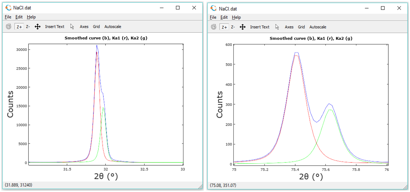
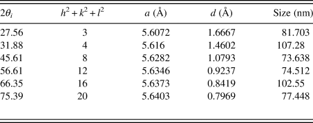
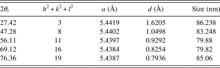
After considering the appropriate experimental setup for XRD data acquisition, the user can execute the main.m routine to calculate properties of specimens. Here, we tested NaCl, Si, and sputtered Au thin-films. Figure 1 shows results for NaCl. Intensities of raw data, as well as K α 1 and K α 2 are shown for comparison in two representative peaks. In addition to this, it is observed that a strong line broadening exists which is likely because NaCl is mostly composed of small size crystallites (Figure 1). Tables II and III show the calculated properties for both NaCl and Si, respectively.
Integral breadth analysis for NaCl for two representative peaks. The blue line contains the original data points, while the red and green lines represent the separated K α 1 and K α 2 intensities.

NaCl solution: FCC crystal system, a = 5.6273 Å, V = 178.2 Å3, APF = 0.74078.

Si solution: diamond cubic crystal system, system, a = 5.4112 Å, V = 158.4 Å3, APF = 0.74078.

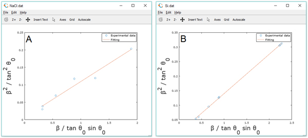
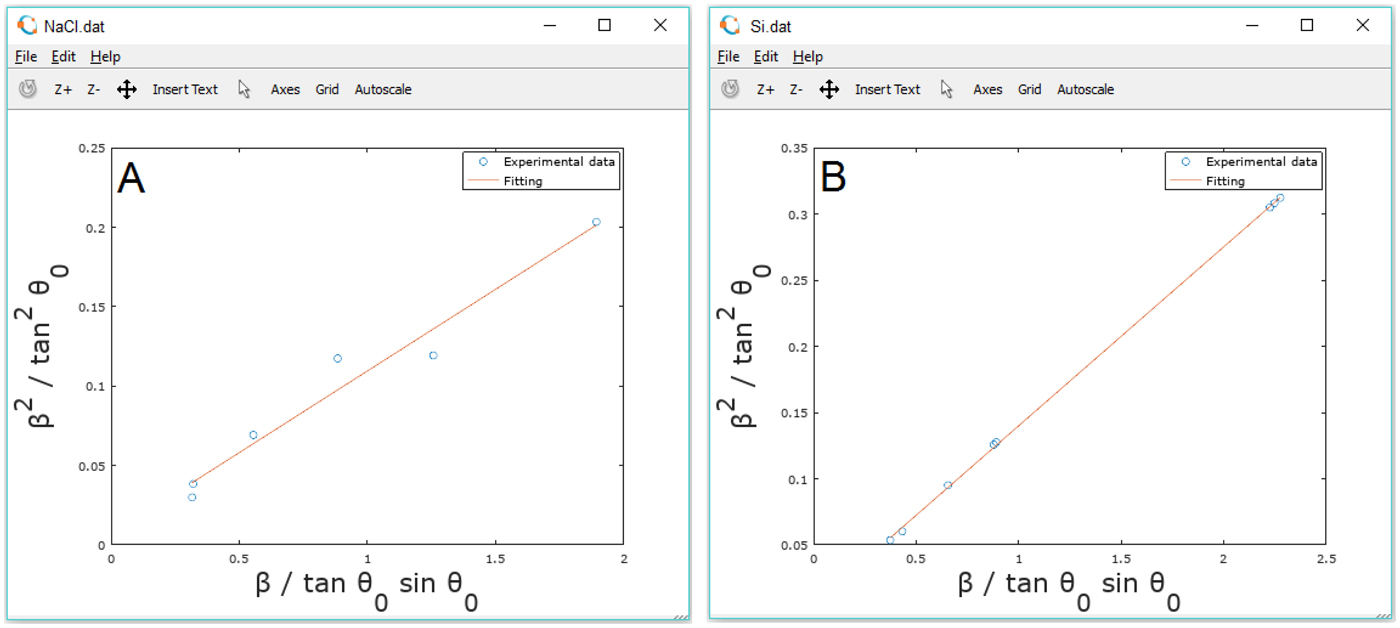
The integral breadths (β hkl) of individual hkl-reflections were determined and plotted as a function of the projection of a diffracting plane normal onto the basal (cross-sectional) plane. From Figure 2, it is observed that the integral breadth does not depend monotonically for NaCl, but a trend is visible for epitaxial Si. Under such circumstance is important to perform a calculation of contrast factor in NaCl to obtain information of strain through the modified WH or WA methods.
Integral breadth analysis for NaCl (A) and Si (B). The red lines indicate the linear fitting.
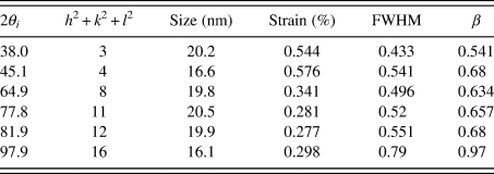
Determination of cell type and peak indexation for Au thin-films are computed using a comparison with a database of cubic crystal structures located in the file cubix.m. Broadening measurements are computed with simple methods: linear interpolation of data for FWHM and integration by a trapezoidal method for integral breadth. Crystallite size and lattice strain at zero order are computed using the calculated Integral breadth formula substitution. Table IV shows the calculated properties on a gold thin film prepared at 400 °C using radiofrequency (400 RF).
Au (400 RF) solution: FCC crystal system, system, a = 5.4112 Å, V = 158.4 Å3.

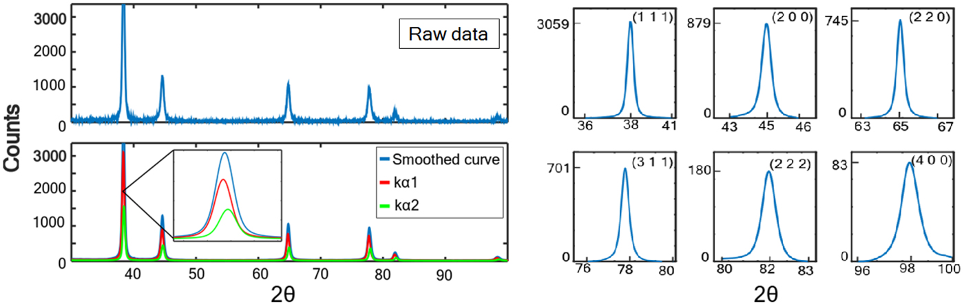
Preliminary diffraction patterns recorded on the Au thin-films indicated a strong preferred orientation in the [111] direction perpendicular to the substrate. After raw data processing, smoothing and K α 2 removal, the peaks can be separated individually as shown in Figure 3 (right) for a further Warren–Averbach analysis.
Diffraction profile (left) and the observed diffracted peaks from Au thin-film (right). The red lines and green lines indicate K α 1 and K α 2 contributions.

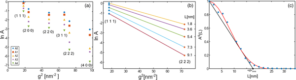
Fourier coefficients of the total intensity are shown in Figure 4(a). The natural logarithm of the DFT of the normalized intensity, L, is shown in Figure 4(b). In order to compute the mean column length d, the polynomial curve
 $$p(x) = (1-ax-bx^2)\exp (-cx^2)$$
was fitted to the A S(L) plot, and the calculation of the tangent line yields the value d at the intersection with the L axis, as shown in Figure 4(c).
Warren–Averbach analysis for Au thin-films.

From Figure 4(c) it is observed that the prepared thin-films show a strong texture that may result in the coherence of X-rays scattered from adjacent nanocrystallites. In particular, a coherently diffracting domain size of about 17.6 nm was calculated in Au thin-films prepared by RF magnetron sputtering. For the same thin-film, the diffracting domain size was calculated in 28.5 nm when using Bragg-Brentano geometry. This result can be related to the low quality of those obtained diffractograms as well as some basic problems underlying the use of bulk models in thin films specimens. Because of the small incidence angle (ω < 1°), the irradiated area on the film surface is large, therefore the diffracted beam is wide which usually yields several times worse peak profile resolution than in the case of focusing Bragg-Brentano geometry.
The microstructure characterization for systems with strain anisotropy require calculations of contrast factors. A subroutine calculates these values according to:
 $$\bar{C} = C_{hkl,0}(1-q\mu H^2)$$
IndexCub allows the selection of a percentage of screw or edge dislocations trough the parameter μ. Contrast factors were implemented accordingly to the previous work published by Armstrong and Lynch (Armstrong and Lynch, Reference Armstrong, Lynch, Mittemeijer and Scardi2004). Computed contrast factors came from routines screw.m and edge.m that are incorporated to extend the WH formalism (currently, IndexCub has no incorporated the anisotropic correction using contrast factors in the WA framework). Thus, a second order polynomial fit is performed to obtain the function containing deconvoluted size and strain. From diffractograms of Au thin-films, it was calculated 13% and 73% of strain respectively when using line profiles obtained with GIXRD and Bragg-Brentano geometries. The high value from BB indicates that line profile evaluation methods may detect a false microstrain broadening. Several studies confirm a correlation between residual stress, stress-free lattice parameter, microdistortions and the size of coherently diffracting domains, it is also known that the variation in peak shape between samples can lead to severe systematic errors as for instance in the determination of strain percentage from modified WH analysis.
VI. CONCLUSION
The basis of a ready-to-use set of routines for X-ray line profile analysis, including Williamson–Hall, Warren–Averbach and contrast factor calculations were described to show the development of an open-source code, IndexCub. As long as modifications on these routines were performed, this task leads to a friendly GNU computational approach based on modules, which are expected to raise a significant understanding of XLPA in undergraduate students. Future works may include methods especially designed for other structures than cubic materials. In the same way, furthermore it is mandatory to increase the usability to allow indexing multiphase patterns as well. The open-source routines can be found online as the Supplementary Material to this article.
SUPPLEMENTARY MATERIAL
To view supplementary material for this article, please visit https://doi.org/10.1017/S0885715619000332
ACKNOWLEDGEMENTS
F.F.C.T thanks Dr. J. Aguilar-Martínez for supporting in XRD experiments for Au thin-films measurements and Dr. R. Cué for preparing the films. This study was partially supported by the National Council of Science and Technology of Mexico (CONACyT, grant 269399).