NOMENCLATURE
- m
size of the Kolmogorov-Zurbenko filter window
- k
Kolmogorov-Zurbenko filter iteration depth
 $a_s^{m,k}$
Kolmogorov-Zurbenko filter window shape
- n
length of matched filter template
- y
matched filter template
- x(t)
section of signal input to the matched filter, of length n
-
$\overline y $
mean value of y


Subscripts
- FETSA
Flight Event Time Synchronous Average
- HUMS
Health and Usage Monitoring System
- OEM
Original Equipment Manufacturer
- RPM
Revolutions Per Minute
- RSR
Regime Signature Recognition
- RTB
Rotor Track and Balance
- RVS
Regime Vibration Signature
- Tacho
Tacho pulse signal (once per revolution)
- TSA
Time Synchronous Average
- 1R
Rotor turn frequency
1.0 INTRODUCTION
During regular helicopter maintenance checks, Rotor Track and Balance (RTB) is often used as a method of minimising the wear on a helicopter’s active components, such as the swashplate and pitch links, by monitoring and modifying the inertial forces of the helicopter blades(Reference Moon and Phan1). The balance of the blades is affected by the physical mass distribution of the blades and their aerodynamic properties, both of which can vary due to minor differences in the blades’ composition, arising from manufacturing tolerances or from operational damage, added marks, etc. Ideally the centre of force of the rotation should be directly over the centre of rotation (the hub) as any offset creates additional out-of-balance forces, ultimately increasing the stress on the mechanisms. There are a number of adjustments that can be applied to the rotorcraft to make sure the rotor is well balanced over a number of typical operating conditions, known as regimes.
1.1 Defining regimes
Regime recognition is the process of deriving the particular flight condition in which a rotorcraft is operating. The first challenge of regime recognition is identifying what classifies as a regime(Reference Renzi2). According to Ref. (Reference Oldersma and Bos3), a regime “can be a flight condition, a manoeuvre or a specific event such as autorotation, [or a] single engine operation [such as] landing,” which leads to the entire rotorcraft flight categorised into these flight regimes as defined by the values of various flight parameters such as ground speed, pitch rate, longitudinal acceleration, vertical acceleration, air speed, weight on wheels, yaw, rate etc.
It is important to note that variations in actual operating conditions are what distinguish a regime from a manoeuvre, such as a hover performed in different wind directions or in-ground-effect, producing several regimes from a single manoeuvre. Ref. (Reference Teal, Evernham, Larchuk, Miller, Marquith, White and Deibler4) uses five fundamental manoeuvres as the basis for their regimes, while other authors have 23 basic manoeuvres or 58 usage manoeuvres(Reference Moon and Phan1). The 58 manoeuvres in Ref. (Reference Moon and Phan1) become 367 regimes when parameters are split into multiple ranges, with even more regimes when the gross weight is split into three categories.
The alternative to this manoeuvre-driven, top-down view of regimes is a parameter-driven, bottom-up approach, where the regimes are determined purely through the combination and granularity of the parameters. In this way, some studies have identified lists of over 1,000 regimes for helicopter flight(Reference Moon and Phan1,Reference Grabill, Brotherton and Keller6) which includes regimes such as climb, left pullout & left turn deceleration, though in this case the number of regimes is reduced to a mere 144 regimes for practical purposes by assimilating similar regimes(Reference Grabill, Brotherton and Keller6). Other studies set a more manageable limit of only 50 regimes, despite an OEM suggestion of 90(Reference He, Wu and Bechhoefer7), or use as few as 8 basic regimes as in Ref. (Reference Rajnicek8).
The large amount of variation in regimes means that the number of flight parameters can also vary considerably, with 40(Reference Moon and Phan1), 37 (including stick positions)(Reference Barndt, Sarkar and Miller5), 7(Reference Grabill, Brotherton and Keller6), 22(Reference He, Wu and Bechhoefer7) and 8(Reference Rajnicek8) parameters in a set as possibilities, although often not all the parameters are needed to identify all the regimes. In most of the literature reviewed, the parameters are not chosen using a truly systematic approach, with one exception where aero-mechanical equations are used to choose the most appropriate flight parameters for identifying a particular regime, as in Ref. (Reference Moon and Phan1).
1.2 Regime recognition techniques
There have been various attempts to detect the current regime from a parameter set, using a variety of techniques, most of which consider the regime recognition as a classification task, specifically as a form of pattern recognition(Reference Wyłomańska and Zimroz9). The simplest of these approaches include setting activation ranges on the parameters such that when all the required signals are within a particular range, the system is considered to be in a particular regime state(Reference Barndt, Sarkar and Miller5), or evaluating the standard deviation, or higher moments, of a single parameter that defines the system to monitor the stability of a current state, a technique used in mobile mining machinery(Reference Wyłomańska and Zimroz9).
In order to discriminate between the potentially large number of regimes requires both a knowledge of the key parameters that can be used to classify a regime, as well as a database of those parameter stored for each manoeuvre that distinguishes a regime. Ref. (Reference Barndt, Sarkar and Miller5) identifies 37 flight parameters and creates a database with over 1,200 regimes, grouped into regime types, though not all parameters are needed to identify all regimes. However, as some other studies only use 22 parameters to identify their 50 regimes(Reference He, Wu and Bechhoefer7), it is clear there is not a simple relationship between the number of parameters and the number of regimes.
The characteristic flight parameter vector of various flight regimes for rotorcraft can be used to train a pattern classifier, such as a neural net, to recognise the individual regimes. Ref. (Reference Celis, Xavier, Teixeira and Pinto10) uses a multilayer perceptron feedforward neural network with backpropagation algorithm, while Ref. (Reference Grabill, Brotherton and Keller6) uses a more complex hierarchical set of 10 neural networks based on eleptic functions to classify a particular flight regime from flight parameter data, though the authors note that the number of networks can be reduced when considering only RTB regimes.
There are a number of other approaches that have been tried: in Ref. (Reference Rajnicek8) a bank of Kalman filters is applied to the flight parameters to estimate a set of indexes, which are indicative of the flight regime. Hidden Markov Models are another approach used in Ref. (Reference He, Wu and Bechhoefer7), where the hidden processes use the current regime and the current measurements to calculate the likelihood of any particular change of regime.
Most of these techniques are preceded by some form of de-noising to improve the results, such as in Ref. (Reference Teal, Evernham, Larchuk, Miller, Marquith, White and Deibler4) where the authors use data filtering, data smoothing and outlier removal to increase the classification accuracy. When there are a larger number of regimes, and therefore potentially a large number of output values to deal with, a decision tree is used to make a final judgment about the current regime, usually using some form of hierarchical decimation(Reference Laillet11).
1.3 Efficacy of current techniques
The accuracy of the approaches mentioned in the previous section varies between 33% for some neural networks, up to 99.94% for the Hidden Markov Models used in Ref. (Reference He, Wu and Bechhoefer7). While on the surface some of these results are impressive, further investigation shows that they are trained for a very specific case, and tested on the very same case.
In addition to these questions about the repeatability or accuracy, all of the techniques presented so far have one of three challenges to address:
Difficulty in acquiring input parameters
Some of the flight parameters are difficult to acquire, either because they are restricted access from the flight computer of the helicopter or because they are not measured as part of the standard configuration, such as stick position, requiring dedicated and inconvenient sensors to be added to the structure. Some parameters are also difficult to measure in the first place, and are estimated by an operator, such as the Weight-On-Wheels signal or the gross weight.
Tight thresholds
The process noise determines the uncertainty in regime recognition. The discrimination thresholds in the case of fine granularity can be very tight, which leads to overlap in the parameter threshold that define a particular regime.
Overfitting in presence of noise
As the level of process noise is usually very high when training a learning system, such as a neural network, it becomes part of the neural model and later when presented with new measurements the classifier may fail by recognising noise as belonging to a certain regime. This overfitting is a well known problem in learning system, especially neural networks(Reference Bishop12).
Compared to the complex solutions discussed so far, this paper will lay out novel technique, referred to as Regime Signature Recognition (RSR), for regime classification that only requires a single real-time signal input to classify the current regime for RTB flights, that uses the system vibration, as well as a new technique for representing any real-time flight signal that extends the visibility of the signal behaviour within a flight.
2.0 METHODS – DATA SPECIFICS
The data used in this paper were collected from an Agusta Westland A109 Helicopter, over a series of three standard RTB flights. During each flight, various channels of data were collected, including four channels of vibration data using a Heltitune® RT6 on-board data recorder. The four vibration channels were designated as Main Rotor Vertical, Main Rotor Horizontal, Tail Rotor Axial & Tail Rotor Lateral, the attributed names reflecting the transducer positions, and are the main data streams used for RTB analysis. The primary signal used here is the Main Rotor Vertical which was located in the footwell of the co-pilot’s seat.
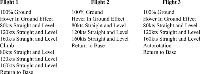
There are five regimes required in a standard RTB test for this aircraft: 100% Ground, Hover IGE (in ground effect), 80kts Straight and Level, 120kts Straight and Level & 160kts Straight and Level. As shown in Table 1, the A109 performed at the very least one complete set of the regimes per flight, with an additional set of the Straight & Level conditions in Flight 1. There was also at least one occurrence of an Autorotation event in Flight 3 and a Climb event in Flight 1. The details of each of these manoeuvres, including the start and end times of these duration events, were manually identified and recorded by a human in a Flight Log for each of the flights. Usually this would be the pilot, thought in this case it was a member of the research team with experience of flight regimes. Note that a duration event is a flight event that has a recorded start time and end time.
List of duration events recorded for each RTB flight used in the study

3.0 DATA PROCESSING
3.1 Overview
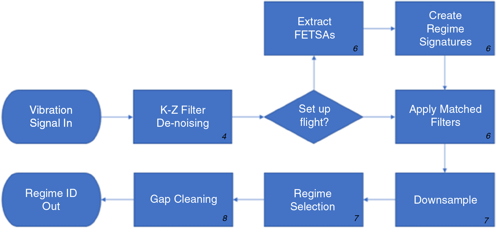
Figure 1 shows a summary of the Regime Signature Recognition (RSR) algorithm. Most of the techniques used in the individual steps of the process are well documented in the literature and will not be covered in detail in this paper, though the effect of each stage as applied to this data will be demonstrated. The techniques that are specific to the RSR are the extraction of the regime signatures and their precursors, the Flight Event Time Synchronous Average (FETSA), which will be explained in more detail. A new visualisation technique will also be presented as an intermediate stage in the development of the RSR technique.
Overview of the Regime Signature Recognition (RSR) process. The number in the corner of each stage indicate the page in this paper where the details of the stage can be found.

3.2 Denoising
Initially all the incoming signals exhibited noise due to the nature of the recording environment, especially for transducers sat directly on active components such as the main gearbox, so a Kolmogorov-Zurbenko filter was applied to each vibration signal. The Kolmogorov-Zurbenko filter can be described as the iterative application of a moving average filter(Reference Yang and Zurbenko13), defined by:
 \begin{align}{\rm{K}}{{\rm{Z}}_{m,k}}\left[ {X\!\left( t \right)} \right] = \mathop \sum\nolimits_{s = - \frac{{m - 1}}{2}}^{\frac{{m - 1}}{2}} X\left( {t + s} \right){\rm{\;}} \times {\rm{\;}}a_s^{m,k}\end{align}
where m is the size of the window, k is effectively the iteration depth, as the filter can be considered as being repeatedly applied, and  $a_s^{m,k}$
is the window shape(Reference Zurbenko14).
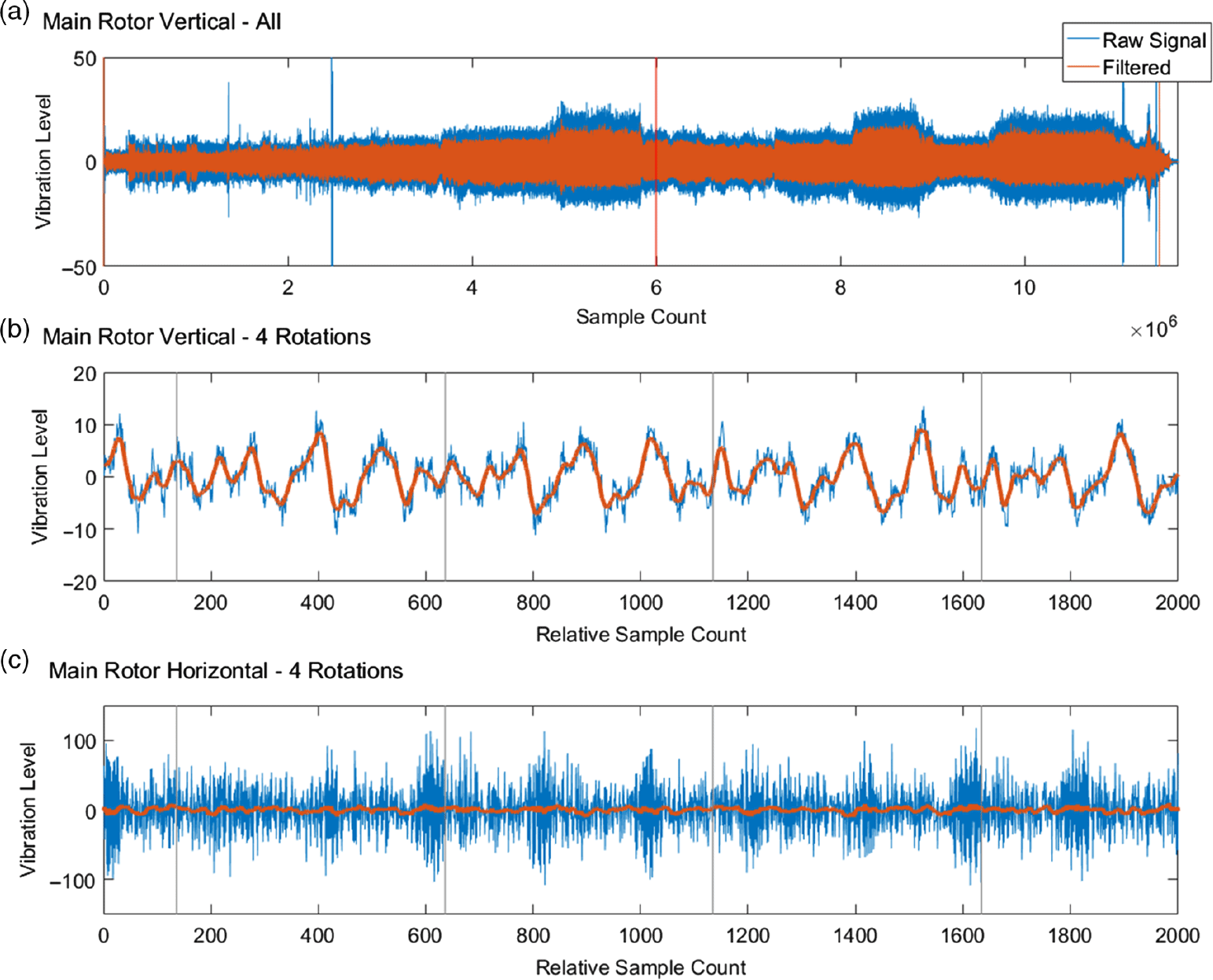
The filter is designed to find discontinuities or level shifts in very noisy data, behaving like a very low pass filter to reveal the general trend of the signal and belongs to the general family of moving window average filters, making it amenable to this application. Figure 2 shows the effect of applying the filter to both the very noisy Horizontal and more quiescent Vertical vibration signals from the main rotor: both result in a smooth signal with an obvious set of low frequency peaks that seems to coincide repeatedly with the Tacho signal, the once per hub rotation (grey lines).
Example of the de-noised vibration signal using the Kolmogorov-Zurbenko algorithm. Figure (a) shows the whole vibration signal for the Vertical Main Rotor vibration channel, while (b) shows a small section of the whole signal (indicated by the red line in (a). The grey vertical lines in (b) and (c) indicate the start of a full rotation of the main rotor hub. While it may seem that little cleaning is needed to see the blade pulses in waveform of (b), for a sensor close to the gearbox and therefore saturated with noise, such as in (c), the de-noising makes these low frequencies much clearer.

3.3 Rotorgram
It is quite clear from Fig. 2(b) that there are four equally spaced peaks between tacho pulses, representing the blade passing frequency, when each blade passes over the same location in turn. It is not known if these beat shapes are constant throughout the flight, or for how long they remain stable before taking on a different deflection shape, because of a shift in aerodynamic forces. One way to visualise these beats for an easy comparison across a flight is to cut the signal into an array of single rotation lengths, and stretching the individual sections to be the same length before stacking them orthogonally to produce a two-dimensional array of values.
Note that because the rotor speed is typically consistent within +/− 2% of the maximum RPM (except for the initial run up and run down conditions) each rotation is typically only a few samples longer/shorter than the average. To reduce the processing burden of interpolating each rotation, only sections with a length difference of more than 5% of a typical rotation are resized, using a simple linear interpolation, while the remainder are either cropped or padded for the few extra samples. Five percent is used in this case because the A109 actually has two speed conditions that it enters for a prolonged duration, and this 5% covers the +/− 2% limits in both conditions. This approximation still results in less than 1% discrepancy in array values compared to the fully interpolated array, and requires far fewer calculations.
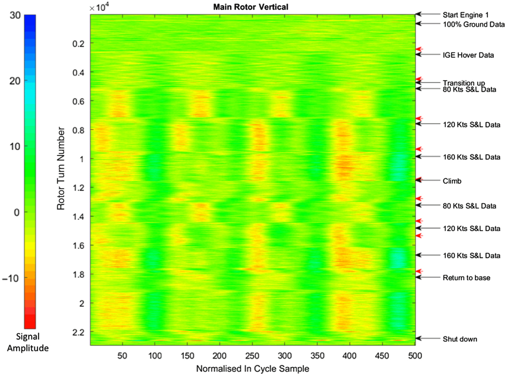
When this array is displayed as a heatmap, with signal amplitude displayed as false colour, as in Fig. 3, it becomes a useful visualisation of the behaviour of the blades over the flight time, which is introduced here as a ROTORGRAM. The important point to note about the rotorgram is that both dimensions are time based: The y axis represents the flight time-line, here as the rotor turn count, from the beginning of the flight (top) to the end (bottom). The x axis represents the time within a single rotation, or the proportion of the full rotation completed, within a scale −Π to Π. Both axes can be represented as alternative units.
The rotorgram for the whole flight, showing changes in the behaviour of the blade within a single full rotation (right to left) as the flight progresses (top to bottom). The labels on the right side indicate flight states as recorded in the log. The black arrows are the start of an event, while any following red arrow shows the point at which it ends. N.B. some flight conditions only happen instantaneously and so do not need an end arrow. The bar on the left shows the true signal amplitude represented by the colour levels in the rotorgram.

From the rotorgram in Fig. 3, it is clear that the blade beats do not remain constant at all times within the rotations as the flight progresses. Instead there are sections of flight where the blade beat profile is consistent, usually connected by visibly distinct transition points. By comparing these consistent profile sections to events in the flight log (right side, Fig. 3), it becomes apparent that the profile transitions often coincide with the start and end of the flight event recorded in the log, and in particular the flight regimes for RTB.
There are some notable exceptions, such as the Return to base regime, where a status transition very definitely occurs within this regime. Return to base however, is not considered a full regime, as it is really only a description of an event, rather than a flight control setup as with the majority of the other regimes, especially those directly connected to RTB.
3.4 Extracting the flight event time synchronous averages
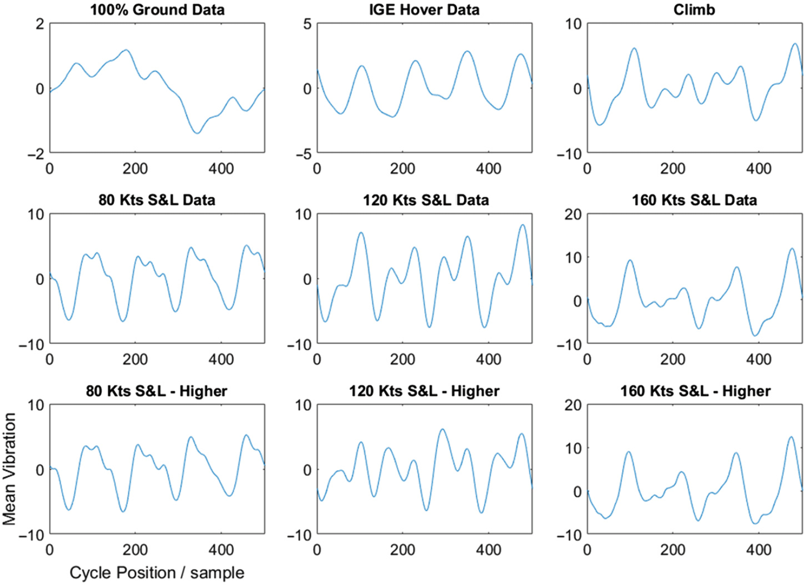
The constancy of the signals within flight events seen in Fig. 3 suggests that each rotation conforms to a standard profile, with some noise, and that by applying the Time Synchronous Average (TSA)(Reference Bechhoefer and Kingsley15) to the whole of a duration event will produce a signal that shows the typical behaviour of the vibration signal within a particular event. These signals are established here as Flight Event Time Synchronous Averages (FETSAs), and are constructed by averaging the rotorgram hub rotation signals using the central 90% of rotations from a flight event. The results of the FETSAs for Flight 1, are shown in Fig. 4.
The Flight Event Time Synchronous Average (FETSA) for each RTB regime identified in the flight log. Note that the axes are the same for each of the individual plots.

3.5 Regime signatures
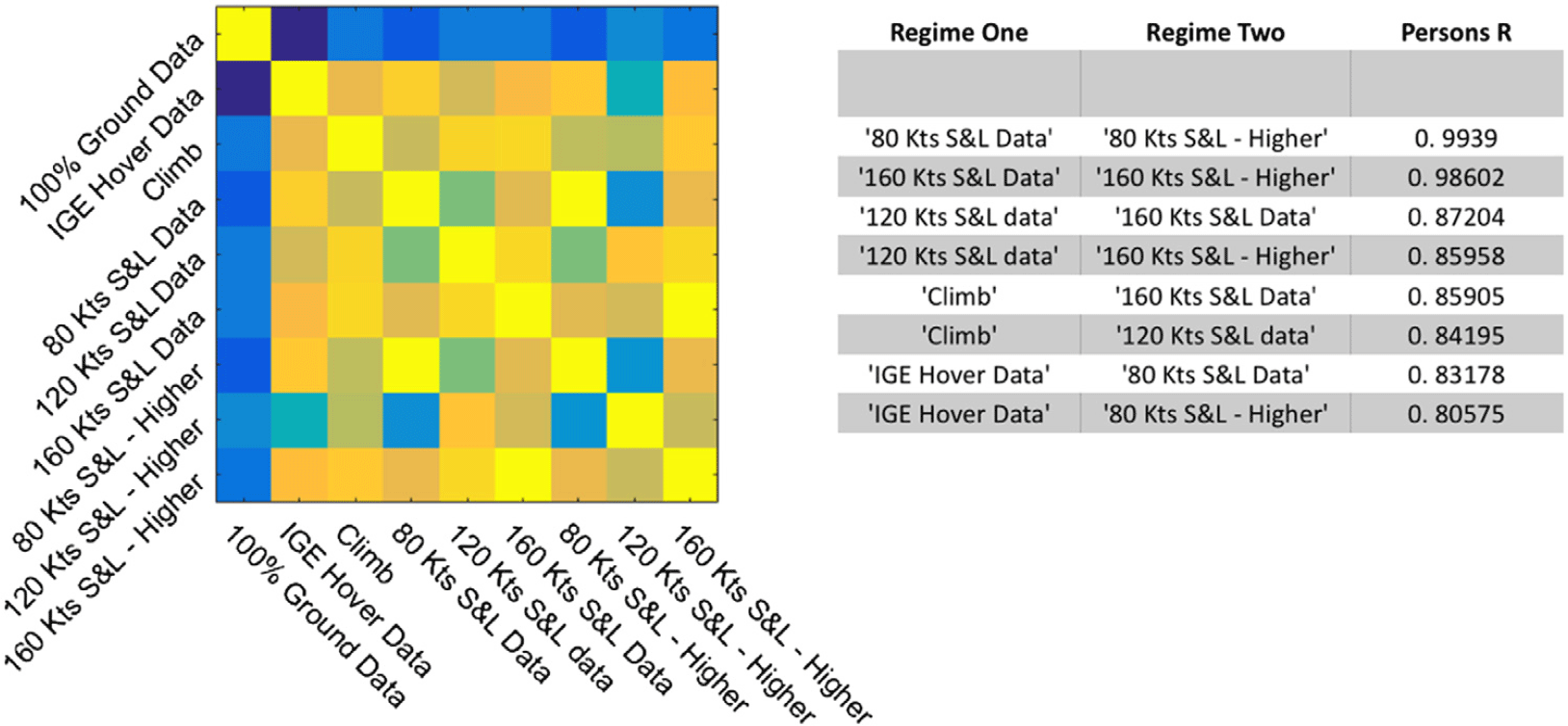
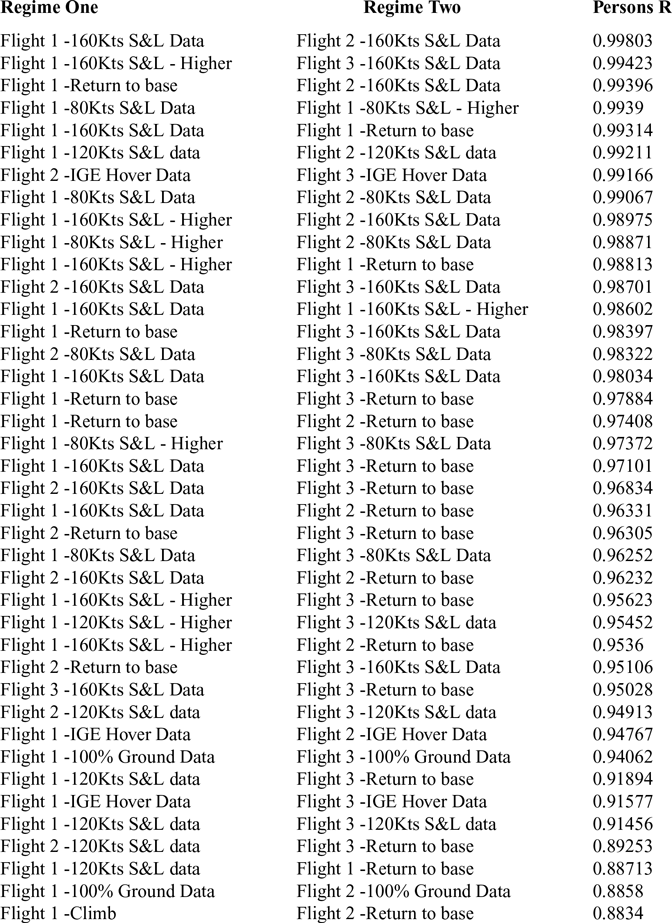
It is apparent that each flight event has a distinct profile, though the underlying blade beats are still clearly visible even after averaging over the thousands of rotations within each regime. However, it is also clear that within this distinctiveness, flight events of the same regime type have very similar FETSAs. This visual similarity can be formalised by performing a cross-correlation of the FETSAs, the results of which indicate that for Flight 1, the correlation between separate FETSAs of the same regime, r > 0.98, while other comparisons are substantially lower (r < 0.88) (Fig. 5). The very high correlation in general is probably due to the underlying four blade beat signal present in every FETSA. These relationships continue to hold true when comparing the FETSAs between flights, as shown in Table 2: There is a similar drop in correlation in all types of comparison, suggesting that each regime has a characteristic FETSA, despite minor variations between flights. The similarity allows the FETSAs for the same regime to be combined to produce a characteristic Regime Vibration Signature (RVS), which can be used as a template to compare against the incoming signals and potentially identify a given regime.
Flight 1 Regime TSA correlation for Flight 1. The full correlation matrix is shown on the left side, with the correlation value indicated by the colour bar in the centre. The results of correlations greater than 0.80 are shown on the right.

Table of the highest inter-flight regime correlation comparisons.

Note that until the last few, the only unwanted correlations are with the Return to base regime, which is an amalgamate of some of the other conditions. The table is truncated at the point where other unwanted correlations stat to appear.
3.6 Matched signatures
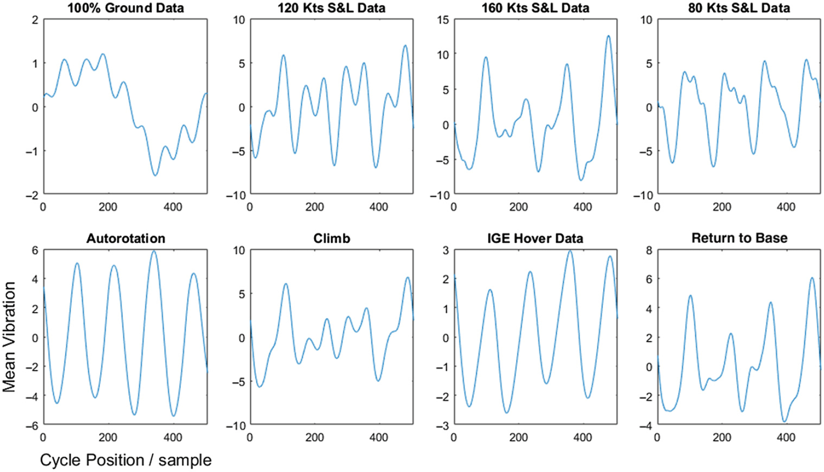
Figure 6 shows the calculated Regime Vibration Signatures for eight flight events: the five RTB conditions, plus the Climb and Autorotation events. Return to base is included simply because it is a duration event, but has no meaning as a regime because it can incorporate a number of true regimes, as seen in the rotorgram (Fig. 3). By comparing the incoming flight vibration signal to these RVSs, it is possible to determine an estimate of the likelihood for each of the possible regimes.
One way to perform this comparison is to take the rotorgram and perform a Pearson’s cross-correlation on each of the rows against each of the signatures, essentially producing eight values per tacho pulse. This approach is possible because of the approximately fixed rotor speed used in the rotorgram and so each single rotation has the same number of samples as the signature. The Pearson’s cross-correlation is used because it normalises the distributions of the two signals values by the signal content, compared to simple linear correlation, meaning that only the match to the shape of a signature and not the amplitude is considered, equalising the signals that feed into the decision-making stage.
The proposed Regime Vibration Signatures (RVS) for eight flight condition. These signatures are created by taking the FETSA’s from all three flights and averaging across all cases of a given RTB regime.

An alternative is to use a technique from signal detection theory called matched filters(Reference Turin16), used to detect specific binary signals in very noisy data. A matched filter uses a bank of filters to compare an incoming signal with various template signatures, creating one filtered stream per template, with the largest stream value at any one point in time indicating the best match of a template. The technique exploits the relationship between correlation and convolution, passing the incoming signal through a bank of shaped filters that are based upon templates taken from the RVSs. A small algebraic rearrangement is required to implement a Person’s correlation rather than a linear correlation, resulting in the standard correlation filter becoming:
 \begin{align}F\left( t \right) = \frac{{y \otimes x\left( t \right)}}{{\sqrt {\sum {y^2} - n{{\overline y }^2}} \sqrt {\sum x{{\left( t \right)}^2} - n{{\overline {x(t)} }^2}} }}\end{align}
Where y is the filter, an inverted version of the template, and x(t is the equivalent length section of the input signal at time t. The means and summations can be calculated by using additional convolution filters, or in the case of the signatures they can be calculated ahead of time and implemented as a constant scaling factor. It can be considered as a convolution normalised by the standard deviations of the two signals, or least-squares normalised convolution.
By passing the new incoming signal through a bank of these RVS based filters, the result is a set of eight time-domain signals that represent the instantaneous correlation between the incoming signal and a particular regime signature.
3.6 Downsampling
The output from the filter bank needs to be down-sampled to produce a single value per channel per rotation that represents the best correlation for the signature. The principles of the matched filter and correlation means that the optimal point to indicate the level of signature matching is the point in the middle of the correlations, i.e. the antiphase of the tacho pulse. However, because the filter itself results in an output delay of half a signature/rotation period when the system runs in real time, this sample point effectively now coincides with the tacho pulse marking the end of the rotation, which is then used to down-sample the matched filter output to the same length as the equivalent block-wise correlation signal.
3.7 Classification
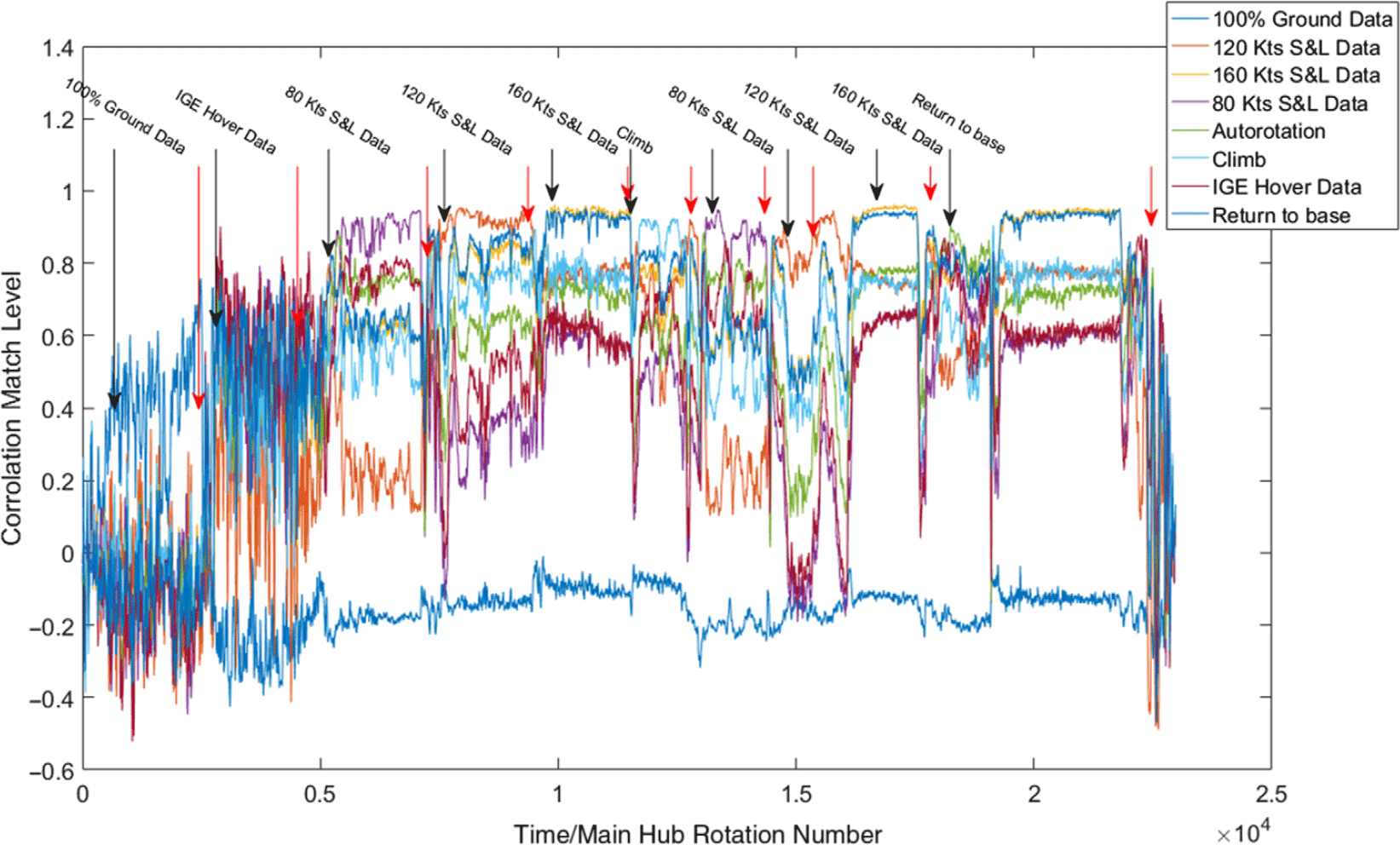
The final stage of a matched filter is to make a decision as to which of the possible templates provides the best match for the incoming signal(Reference Turin16). Ideally a simple winner-takes-all or maximum value classifier would be acceptable and Fig. 7 shows that for about half the flight regimes there is a clear and correct winner (80kts S&L, 120kts S&L, etc.); however, there are flight conditions that either have two very close candidates for maximum value, such as 160kts S&L vs. Return to base, or sections where the profile signal is so noisy it might jump below other signals (i.e. IGE Hover).
The Matched Filter results for Flight 1 using the signatures in Fig. 6. This graph shows the output from applying the matched filters to the Main Rotor Horizontal, and performing the down-sample. The regime labels across the top indicate the start and end of RTB regime in the flight time as before.

An alternative option is to use a simple learning system, such as a neural net, to make the choice. The advantage for using such a system is that if there are two signals it is difficult to distinguish between simply using their own matched filter values, it may be important to take into account the current level of other profiles that might add to the weight of evidence in one direction or another. For example, Fig. 7 shows that the Autorotation signal is clearly lower in the Return to base condition than for 160kts S&L.
The neural network implemented here was a simple back-propagation configuration: a single hidden layer with ten nodes. There were 16 input nodes, as the matched filter results from two channels (Main Rotor Vertical & Main Rotor Horizontal) were included to improve the accuracy, and nine output signals, including a generic flight regime called Unknown, used to cover any part of the timeline not associated with a regime, such as transitions. The network was implemented in Matlab® using the Scaled Conjugate Gradient Algorithm(Reference MØller17) as the training algorithm.
The network was trained using a sample set of data that had been passed through the matched filter templates. These data were the raw vibration signals that had been used to create the signatures, and half of these data points were used as the training set. The remaining data points from the matched filter were then used as a holdout set to test the output of the neural network.
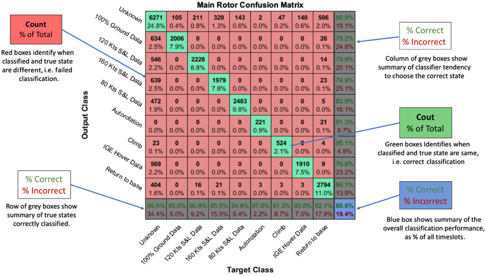
Figure 8 shows a typical confusion matrix from this training-testing cycle, which was repeated 100 times to confirm the stability of the classifier. The confusion matrix is a technique to show the success rate of the classifier split by confusion between the true regime and the classifier’s output. It not only shows the overall success of giving the correct regime, but also useful for identifying what causes the classifier to become confused. In Fig. 8, the green boxes on the diagonal indicate the correctly classified rotations, while the numbers in the boxes indicate the total number of these correct classifications, with the percentage of all classifications underneath. Red boxes indicate incorrect classifications, with the same values inside. The system successfully identifies the correct regime 80.6% of the time, compared to a simple chance rate of around 11%, with absolutely no confusion between RTB regimes. It is clear that most of the incorrect classifications are due to confusing the RTB regimes with the Unknown condition, with a smaller contribution from Return to base. This is not unexpected as these two regimes are an amalgamation of regimes from the extended set, and therefore likely to be confused with other regimes.
Example confusion matrix for a neural network trained using the match filter outputs from all flights. Data from half the time slots (randomly selected) on both the main rotor signals were used to train the network, and the remaining data was used to produce this particular confusion matrix. Each row represents the classification made by the computer classifier, while each column indicates the true state of a particular time slots. Note that there are no false classifications between the true regimes, only in the mixed regimes of Return to base and Unknown are confusing results produced.

It is noted by the authors that there are many varieties of decision making techniques, including many of those mentioned in the introduction, and each of them have many variations in methodology. This result, derived from a basic classifier, illustrates the strength of the core RSR technique, independent of the classifier used in this final stage.
3.8 Gap cleaning
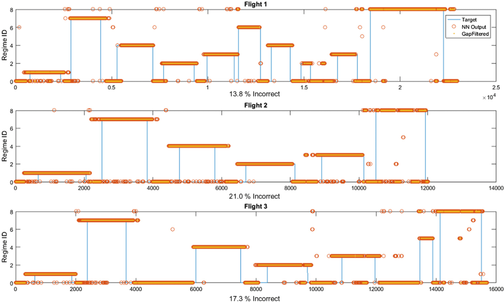
The output from the neural net is performed as if each point is independent, with no regard for which regime an adjacent point has been classified as. This leads to the result shown by the red circles in Fig. 9, where for all three flights, there are many occasions when a single time point is misclassified breaking up a continuous regime. Some of the techniques for decision making can incorporate a temporal element into its processes, but here a simple binary smoothing is used to remove any gap in a regime of less than ten rotations, approximately two seconds in real time. Note that while further processing could be used to make sure that adjacent conditions are valid, such as knowing a transition from Hover IGE to 160kts S&L is not possible, the nature of the real regimes mean that there is always a transitional period between regimes, with blade beat patterns that do not match any known regime. For this reason, small gaps are filled in on the basis of individual regimes, and the transitions between regimes are assumed to have large gaps of unidentified signal.
Plots showing the classification levels for each flight as recorded, showing the level of classification achieved by the neural network classification of the match filter signals, and the smoothing produced by the gap filter. The blue line shows the flight condition as recorded in the log. Note that just because that is when the log states a condition ends is not the same as the helicopter actually changing state, which is why a large proportion of the incorrect classifications are type 1 errors: i.e. the classifier is not actually incorrect, but the log itself is inaccurate.

To perform this gap filling, the signal is split into nine binary signals, each representing whether this regime is the current regime or not. Gaps of fewer than ten samples are filled in with the value of the preceding sample status (i.e. gaps of 0 values are set to 1, and visa-versa), and the signals are recombined. Any conflict between regime during the recombination is considered to be during a transition and reclassified as the Unknown regime. The orange dots in Fig. 9 show the smoothed outputs, demonstrating how most of the RTB sections are now completely solid, with almost no instability in regime identification.
4.0 FINAL RESULTS
Figure 9 shows how the final output from each flight compares against the log information, with the percentage of incorrectly identified regimes displayed underneath each graph.
A large number of the identified RTB regimes extend beyond the start and end of their recorded existence, creating a number of false positives for a particular regime. This feature is probably due to the recording method of the flight log, i.e. human input. Ref. (Reference Teal, Evernham, Larchuk, Miller, Marquith, White and Deibler4) attempts to remove human variability by using multiple pilots, while Ref. (Reference Moon and Phan1) notes that the control stick position is not used directly for recognising manoeuvres, effectively disconnecting the pilot behaviour from the current regime as measured by the instrumentation. In the case of the flight data presented here, the log is representative of when the person recording the event is certain that the rotorcraft is within that condition, meaning recorded times and durations are likely to be conservative. The aircraft may very well have actually been in a defined regime for a period before it was officially recorded.
There are still a few prolonged periods where the system has produced a different regime classification to the flight event. This may be where improvements in the algorithm need to be focused but it is also possible that for these sections of the flight the conditions actually changed, such as a heavy gust that would change the air speed without warning and therefore change the flight condition, which might invalidate any RTB measurements.
These problems are more of data collection than of processing, and it is intended that as this investigation extends to more flight regimes, both the algorithm and the method of collecting the relevant data are refined.
4.1 Signal combinations
While the majority of the paper focuses on the signature properties of the signal from a single transponder, combining the transponder signals might be a good way of improving the performance. For example, there is a 4% improvement in the performance of the system if the input to the neural network is fed by the matched filter result signals from both the horizontal and the vertical transducer. Combining the tail rotor transducer signals in this way produces a similar result, though combining the signals from the main rotor and the tail rotor to extend this result is problematic as they are asynchronous. The classifier demonstrated in the final section of this paper uses the combination of the vertical and the horizontal, as it produces the best result for the presented methodology.
4.2 Effect of noise
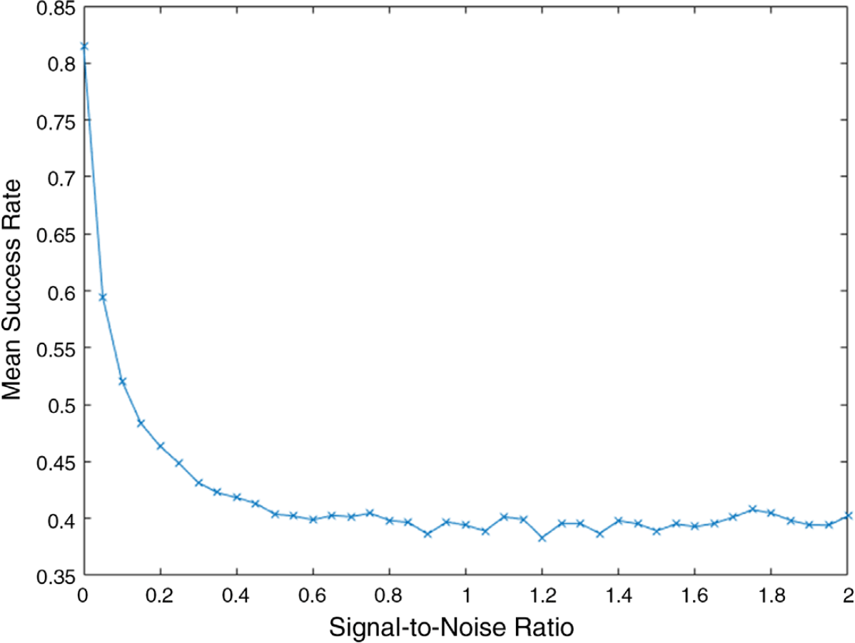
The combination of signals produces a small gain in accuracy, but there is potential for large losses of accuracy if there is noise on the original signal. Figure 10 shows the effective robustness of the system in different levels of noise, as a comparison between success rate and Signal-to-Noise ratio (SNR). The system was repeatedly trained using the original denoised signal Matched Filter results, then tested by applying the whole process to signals with an increasing SNR. These noisy signals were created by adding normally distributed random data to the original denoised signal, with the maximum amplitude reducing from 2 to 0. The increases in noise almost exponentially reduce the success rate of the technique, though there are two factors that should be accounted for in this test: First of all, the denoising will normally be applied to such signals reducing the SNR somewhat again. And secondly, there may be more nuanced differences that the neural network was not trained to pick up on between the results of the matched filter.
Demonstration of the effect of noise in an input signal. Plot shows the mean success rate of ten iterations of training the neural network on the processed signals from the denoised data, and tested on processed signals with various signal to noise ratios. The SNR was manipulated by adding Gaussian white noise to the denoised signal, with increasing amplitudes of noise to change the variance. Plot shows the noise as ratio to signal, as the denoised signal would be considered to have SNR = ∞.

5.0 CONCLUSIONS
This paper has shown a new, intuitively informative visualisation of the vibration data that comes from the Health and Usage Monitoring System (HUMS) time domain data. This Rotorgram visualisation makes it possible to see the behaviour of the blades as the flight progresses and any meaningful fluctuations, possibly even allow an operator to observe lead-lag or deflection changes. More work is currently being carried out with ground crews to see if this basic visualisation can lead to better on the ground insights during maintenance periods.
The development of the Rotorgram has also led to the creation of the Regime Vibration Signature (RVS), a characteristic 1R (single rotation) time domain vibration signal wave form that can uniquely identify the current regime. Using these Regime Signatures, the authors have presented a novel methodology for identifying the RTB regimes while in flight, using a number of existing signal processing stages to analysis vibration data.
The RVS methodology is based around the use of matched filters to compare the incoming signals to the respective Regime Signatures. This core process is supplemented by some other stages to perform operations of Denoising, Creating the Signatures, Down-sampling, Decision making and Gap Filling. A summary of the components in the current implementation of the methodology are shown in Fig. 1 and has demonstrated an 81% successful regime recognition rate, compared to an approximately 11% chance level.
The main advantage of this technique is that it can be constructed from a single, tangible, vibration signal once set up, rather than requiring the input of many process parameters, some of which either have to be inferred or rely on human input. Additional advantages are that it has an understandable representation in the system, unlike some types of learning system that overly abstract the information, disassociating the result from the physical system that the ground crew have to consider, or what the result means for the system.
There is still much work to be done to probe how the Regime Signatures behave over a wider range of circumstances: changes over time, variance between aircraft or weather conditions, or distinguishing between an extended set of regimes. These results will give a better understanding of how unique the signatures are to the aircraft, and how much tuning is required to apply this technique to a brand-new aircraft. It expected that the technique will have its limitations, but will provide a viable and understandable starting point to develop operational flight RTB techniques, an important goal in the current rotorcraft industries.
ACKNOWLEDGMENTS
The authors would like to thank Innovate UK and Helitune for funding the research that this paper comes from. The authors would also like to thank Castle Air and Prosig for their help in acquiring the data in a format that was useable.