Introduction
The mass balance of the Antarctic ice sheet is receiving increased attention due to its relevance for climate change studies and sea level contribution (Jacka et al. Reference Jacka2004). Mass balance methods applied in Antarctica include the mass budget approach where snow accumulation input is compared to ice flow output (Rignot et al. Reference Rignot, Bamber, van den Broeke, Davis, Li, Van de Berg and van Meijgaard2008); repeated altimetry using airborne and satellite data obtained by radar and laser sensors (Smith et al. Reference Smith, Bentley and Raymond2005, Wingham et al. Reference Wingham, Shepherd, Muir and Marshall2006) to measure ice elevation changes; and determination of temporal changes in gravity based on satellite data (Velicogna & Wahr Reference Velicogna and Wahr2006). Recent assessments suggest an overall negative mass balance for Antarctica, with sea level contribution values that range from -0.14 to + 0.55 mm a-1 (Lemke et al. Reference Lemke, Ren, Alley, Allison, Carrasco, Flato, Fujii, Kaser, Mote, Thomas and Zhang2007). A growth in East Antarctica probably caused by increased snowfall (Davis et al. Reference Davis, Li, McConnell, Frey and Hanna2005) seems to be offset by larger shrinkage from West Antarctica and the Antarctic Peninsula due mainly to enhanced flow, associated thinning and enhanced basal melting of ice shelves (Rignot & Thomas Reference Rignot and Thomas2002, Rignot et al. Reference Rignot, Casassa, Gogineni, Kanagaratnam, Krabill, Pritchard, Rivera, Thomas, Turner and Vaughan2005, Shepherd & Wingham Reference Shepherd and Wingham2007). While two satellite radar altimetry studies suggested an overall null or even positive mass balance (Zwally et al. Reference Zwally, Giovinetto, Li, Cornejo, Beckley, Brenner, Saba and Yi2005, Wingham et al. Reference Wingham, Shepherd, Muir and Marshall2006), other studies conclude a substantial mass loss for the continent as a whole but with very high uncertainties (Velicogna & Wahr Reference Velicogna and Wahr2006, Rignot et al. Reference Rignot, Bamber, van den Broeke, Davis, Li, Van de Berg and van Meijgaard2008).
Within the Antarctic, fast flowing ice streams, grounding line areas and ice shelves are particularly sensitive to changes in mass balance. So far mass balance changes in the interior of the continent have been attributed to enhanced snowfall in East Antarctica (Davis et al. Reference Davis, Li, McConnell, Frey and Hanna2005), although this has been disputed by more recent studies (e.g. Monaghan et al. Reference Monaghan, Bromwich, Fogt, Wang, Mayewski, Dixon, Ekaykin, Frezzotti, Goodwin, Isaksson, Kaspari, Morgan, Oerter, Van Ommen, Van Der Veen and Wen2006). Ice sheet areas close to rock outcrops in mountain regions where fixed reference sites can be deployed are especially suited for monitoring changes in elevation and ice velocity using ground-based methods. An additional advantage of mountain regions is the frequent presence of blue-ice areas (BIAs) due to wind erosion and enhanced sublimation (Bintanja Reference Bintanja1999, Sinisalo et al. Reference Sinisalo, Moore, Van de Wal, Bintanja and Jonsson2003), where elevation changes over ice can be measured, avoiding the effects of possible changes in firn densification.
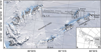
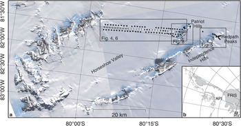
Glaciological studies at Patriot Hills (80°18′S, 81°22′W), southern Ellsworth mountains, were initiated in 1995 as part of the Chilean Antarctic programme. Patriot Hills are located ∼50 km inland from the Ronne Ice Shelf grounding line (Joughin & Bamber Reference Joughin and Bamber2005), on the southernmost margin of Horseshoe Valley (Fig. 1). Mass balance results by means of repeat measurements of stakes at Patriot Hills and Horseshoe Valley performed by optical survey in 1995, and by GPS surveys in 1996 and 1997, have shown that the ice sheet is in near steady state (Casassa et al. Reference Casassa, Brecher, Cárdenas and Rivera1998, Reference Casassa, Rivera, Acuña, Brecher and Lange2004). Here we analyse new elevation data at Patriot Hills and Horseshoe Valley obtained from GPS surveys in 2004/2005 and January of 2006, and compare them with GPS data obtained one decade earlier.
Network survey
In November/December 1996 an existing network of ablation stakes near Patriot Hills (Casassa et al. Reference Casassa, Brecher, Cárdenas and Rivera1998) was extended across the whole width of Horseshoe Valley consisting of three parallel lines with a stake separation of about 1 km (Fig. 1). Additionally, some stakes were set up on the ice cliff between Independence Hills and Redpath Peaks.
The position of all stakes was observed by static Global Positioning System (GPS) measurements of at least ten minutes with geodetic-quality dual-frequency GPS equipment relative to a GPS site in the Chilean base camp “Teniente Arturo Parodi” located on snow, at the southern margin of Horseshoe Valley, about 250 m north of the Patriot Hills BIA. The position of the Parodi base station was determined three times during the campaign, using a reference site on bedrock located 2.6 km to the south-west, on the northern slope of Patriot Hills.
One year later (1997), the complete network was resurveyed by GPS with Leica SR9500 receivers and antenna type LEIAT302-GP, and a slightly modified measurement strategy to allow for shorter observation times. Additionally to the base station established at Parodi base camp, two temporary base stations across the valley were deployed to reduce baseline length to 13 km at the most. These temporary base stations operated for one or two days only, with differential observations lasting 20 and 40 minutes, respectively. All stakes were observed in a stop-and-go mode with observation times as short as three minutes, by means of the Leica GPS receiver that does not record data in kinematic mode but keeps track of the phase ambiguities.
Due to burial by snow accumulation, most stakes could not be found during the following resurvey performed in November/December 2004, as expected. Near the BIA where net ablation prevails, about 10 stakes were found and measured again. In view of the loss of stakes, a kinematic scheme was adapted to resurvey the surface heights at the stake positions. A geodetic site on bedrock in Patriot Hills served as a base station and was operated semi-permanently throughout the whole GPS campaign. For the kinematic survey a Javad Lexon GD receiver and an antenna MarAnt, operating with a sampling interval of five seconds, were mounted on a snowmobile. Around the former stake positions, a regular trefoil pattern of 100 m radius was surveyed to enable the reconstruction of the ice or snow surface height at the exact location.
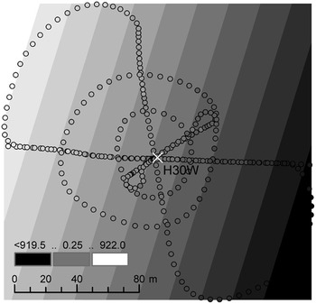
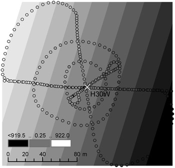
The kinematic survey of the stake locations was repeated in January 2006 with the same GPS equipment as in 2004. The ground pattern around each stake location was slightly modified, now consisting of two concentric circles of about 25 and 50 m radius and two loops of 100 m (Fig. 2). The sampling rate in 2006 was increased to 1 Hz. The few stakes on and near the BIA that still existed were additionally surveyed statically.
Example of survey pattern and plane adjustment to the 2006 kinematic survey around the location of stake H30W.
Data analysis
All GPS data (four epochs) were (re-)processed using the commercial software GrafNav 7.60 to provide for a consistent analysis procedure. We used dual-frequency carrier-phase measurements. For baselines longer than 10 km the ionosphere-free linear combination was employed. The processing of each GPS campaign exhibited some peculiarities which are summarized below.
1996
As mentioned above, the Parodi base station of the 1996 survey was established on snow and thus moved due to ice flow by an unknown amount during the campaign. A baseline to a site on bedrock located at Patriot Hills 2.6 km to the south-west was observed three times to enable the correction of this influence. The resurvey of the 1996 base station in 1997 revealed a flow velocity of 1.1 m a-1, resulting in a displacement of 0.07 m during the three-week campaign. This displacement was finally ignored and the mean value of the three sessions was used as coordinate for the base station. For about 95% of the sites ambiguities could be fixed reliably. The usually too optimistic standard deviation calculated by the software is between 0.01 m and 0.03 m for the vertical component of most sites. As none of the stakes were observed twice, the standard deviation of the coordinates cannot be estimated independently to check for consistency, but a mean vertical precision of 0.15 m was regarded as reasonable.
1997
The observation times of the stakes with a minimum of 3 min in the stop-and-go configuration used in 1997 occasionally proved to be too short for the ambiguity solution within the GrafNav software, especially on longer (> 10 km) baselines. Consequently, 10% of the sites could not be reliably processed. The results from a few repeated measurements of stake sites agree within 1–2 cm in the vertical in case of fixed ambiguities. However, when the ambiguity solution failed, bad float solutions can cause height differences between repeated sessions of the same site of up to 1 m. Special care has been taken to evaluate solutions and reject bad ones, which has resulted in a data gap of 3 km between stakes H17 and H20 within the otherwise evenly spaced profile. Similar to 1996, a mean vertical precision of 0.15 m was considered.
2004
The kinematic processing of the 2004 measurements showed a large number of cycle slips resulting in a heterogeneous accuracy of the epochs. About 9% of all kinematic positions had a vertical standard deviation larger than 0.5 m according to the GPS software and were excluded from further consideration. A reason for this could be the combined effect of the low sampling rate (5 s), the ionosphere refraction and the distance covered between successive observations. The mean vertical standard deviation of the remaining epochs was 0.1 m.
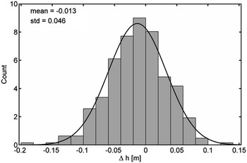
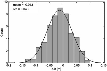
To determine the surface height at the exact location of the 1996 stakes, a plane was fitted to the kinematic positions in a vicinity of 100 m and used for interpolation. At this scale, the terrain in Horseshoe Valley is quite smooth. Only in a few places near the flanks of the valley, the surface is curved and a bilinear approach was used. Another limiting factor is the local roughness that at some stakes can reach 30 cm, but usually the surface is smoother. The resulting approximation errors, which indicate the accuracy that can be expected for the interpolated heights, follow a normal distribution (Fig. 3) and support the validity of this approach. These misfits are both a measure of the validity of a plane assumption in the vicinity of the sites and, in smooth areas; they also serve as an independent estimation of the GPS error.
Approximation error of the plane adjustment shown in Fig. 2. The black line represents the normal probability density function with the same values for mean and standard deviation.
For the 2004 data the accuracy of the height determination varies strongly from stake to stake depending whether ambiguities could be fixed or not. Shorter baselines tend to be more reliable with a vertical misfit of about 0.10 m. The vertical approximation error of distant sites (> 20 km from the base station) can range up to 0.40 m with an overall mean of 0.27 m.
2006
The main difference of the 2006 survey in comparison to that of 2004 is the higher sampling rate of 1 Hz. This resulted in a higher percentage of solved ambiguities and therefore nearly homogeneous solutions. Only in 0.5% of the epochs the vertical error exceeded 0.5 m (vs 9.2% in 2004) and only two days were affected by this, raising the speculation of an intermittent deteriorating effect, e.g. ionospheric refraction.
The mean vertical standard deviation of all kinematic epochs is 0.05 m. The vertical misfit of the adjusting planes amounts to about 0.10 m, ranging from 0.05 m to 0.15 m and depends only slightly on baseline length. Thus, this value can be used as a measure of the standard deviation of the 2006 height determination of the stakes. Figure 2 shows the example of stake H30W at a distance of 25 km from the base station, with an approximation error of 0.05 m.
Results
Ice flow velocities
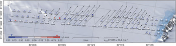
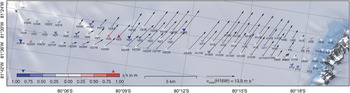
The reanalysis of the 1996 and 1997 data resulted in revised velocities for the profile across Horseshoe Valley (Fig. 4), with near-zero velocities at the edges of the valley and a maximum of 14.0 m a-1 in the centre with uncertainties in the range of 0.2 m a-1. The flow direction is along the axis of the valley, that is, towards the south-east. Casassa et al. (Reference Casassa, Rivera, Acuña, Brecher and Lange2004) obtained velocities ranging from 13 m a-1 near the margins to 25 m a-1 at the centre of Horseshoe Valley, with a mean easterly direction. The reason for the differing results from Casassa et al. (Reference Casassa, Rivera, Acuña, Brecher and Lange2004) seems to be the use of a marker on ice as a moving base station. In their analysis, differences of repeated coordinate determinations for the base station on the glacier relative to bedrock were interpreted as movement, but in fact this only increased the uncertainties.
Ice flow velocities (arrows) and height changes (triangles) in Horseshoe Valley derived from GPS measurements of stakes in 1996 and 1997.
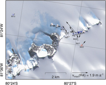
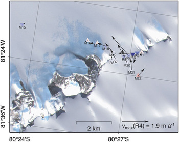
At the ice cliff between Redpath Peaks and Independence Hills, the maximum slope is 6%, with ice flowing from the south down to the valley between Independence Hills and Horseshoe Valley, with a vertical drop of 65 m. Velocities in the ice cliff have a general north-east direction, with magnitudes from 0.3 to 1.9 m a-1 (Fig. 5). The flow vectors of stakes R1 and R2 point to the west, which can be explained because of the local slope on the steep flank of Redpath Peaks.
Ice flow velocities and height changes at the ice cliff between Redpath Peaks and Independence Hills derived from GPS measurements of stakes in 1996 and 1997. For colour scale of the triangles see Fig. 4.
Ice flux through the Horseshoe Valley profile
Based on the revised surface velocities, we re-estimate the annual ice flux leaving Horseshoe Valley combining these flow velocities with ice thickness information. The stake network, which serves as a flux gate, divides the valley cross section into 32 sections each characterized by a mean flow velocity and a mean ice thickness. The integrated flux across the whole profile can then be calculated summing up all individual products of ice flow velocity  , ice thickness H and width of the section W:

The measured surface velocities have to be converted into depth-averaged velocities. The usual approach assuming ice frozen to the bedrock is using Glen’s flow law with a nonlinearity of 3 (Paterson Reference Paterson1994, p. 252) leading to a depth-averaged velocity that amounts to 80% of the surface velocity. Ice thickness information comes from radar echo sounding measurements realized between 1995 and 1997 (Casassa et al. Reference Casassa, Rivera, Acuña, Brecher and Lange2004) and in December 2007 (Ulloa et al. Reference Ulloa, Uribe, Zamora, García, Casassa and Rivera2008). Due to limitations of the 2.5 MHz impulse radar system used in the 1990s, a 10 km wide sector of the profile with ice deeper than 1200 m could not be observed. In 2007, this deep area was measured with a pulse compression radar depth sounder operating at a central frequency of 155 MHz, especially designed for thickness measurements of cold ice (Ulloa et al. Reference Ulloa, Uribe, Zamora, García, Casassa and Rivera2008). The maximum ice thickness measured is 2246 m 12 km north of Patriot Hills. The valley is considerably deeper than the previously extrapolated value of 1520 m (Casassa et al. Reference Casassa, Rivera, Acuña, Brecher and Lange2004).
The profile does not cross Horseshoe Valley perpendicularly so that the widths of the gate sections formed by the stakes have to be projected normal to the valley axis. The revised ice flux of Horseshoe Valley amounts to 0.19 km3 a-1 ± 0.004 km3 a-1. This is about half of the value of 0.44 km3 a-1 ± 0.08 km3 a-1 calculated by Casassa et al. (Reference Casassa, Rivera, Acuña, Brecher and Lange2004), which can be explained by the smaller recalculated ice flow velocities.
Glaciological mass balance analysis
The ice flux through the Horseshoe Valley flux gate comprising the outflow mass balance component can be compared with the input into the valley system from snow accumulation and from influx through the ice cliffs between the hills that separate the valley from the interior ice plateau.
The integrated accumulation in the valley upstream of the profile (1087 km2 ± 100 km2) was estimated by Casassa et al. (Reference Casassa, Rivera, Acuña, Brecher and Lange2004) to be 0.11 km3 a-1 ± 0.04 km3 a-1 considering a net accumulation rate of 100 kg m-2 a-1, which is the mean value determined at the profile. While the uncertainty in the accumulation estimate might account for this discrepancy, the mass balance difference of 0.08 km3 a-1 could also be explained by a moderate additional influx of ice with a mean thickness of 500 m and a velocity of 8 m a-1 across the c. 20 km wide ice cliffs in the west side of the valley (∼80°S, 83°W and 80°10′S, 82°30′W; Fig. 1). In the light of the velocity of 2 m a-1 at the very narrow ice cliff at Redpath Peaks these values might be plausible. Therefore, the flux gate method gives no indication for a significant mass imbalance of Horseshoe Valley. To reduce the large uncertainties of the mass balance determination, ice thickness and velocity measurements at the ice cliffs would be necessary.
Surface elevation changes and geodetic mass balance estimation
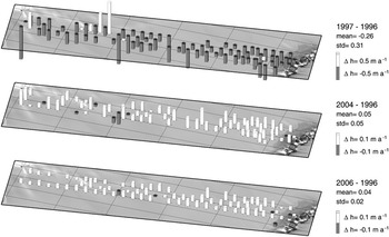
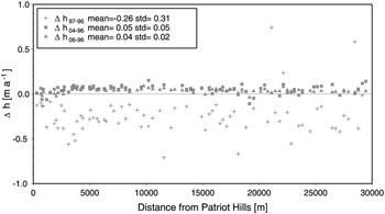
The surface height determined at the stake locations for all four epochs can be used to calculate surface elevation changes (Fig. 6) and to assess the mass balance by means of the geodetic method (Bamber & Payne Reference Bamber and Payne2004). For the 1996–97 comparison, static measurements of actual stakes are available to assess elevation changes. However, due to the ice flux the stakes do not represent the same location in both years and the height difference has to be corrected for surface slope. This can be done using the planes adjusted from the 2006 measurements. The slightly less precise data of 2004 (see above) have been used to adjust planes at the stake locations without measurements in 2006. After performing the slope correction the data show a mean elevation decrease of 0.26 m a-1 for the period 1996–97 and a large scatter (see Fig. 7) either due to a spatially varying pattern across the valley or more likely due to uncertainties in the height determination mentioned earlier. Four stake locations with gross errors were excluded from the further analysis. The mean surface decrease is consistent with the extremely low snow accumulation in 1996/97 in contrast to the previous year, as already reported by Casassa et al. (Reference Casassa, Rivera, Acuña, Brecher and Lange2004).
Elevation change rates in Horseshoe Valley. a. Derived from stake measurements in 1996 to 1997, b. derived from comparison of kinematic GPS survey in 2004 with stake measurements in 1996, and c. derived from comparison between 2006 and 1996.
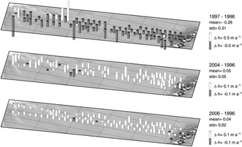
Elevation change rates across Horseshoe Valley plotted along the profile from Patriot Hills towards Douglas Peaks.
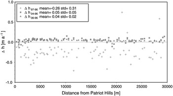
The comparison between the heights derived from the kinematic remeasurement in 2004 and the original stake heights in 1996 (Fig. 6b) does not require a correction for the effect of ice flow as the 2004 measurements were interpolated to the same position where the meanwhile disappeared stakes were installed in 1996. The mean elevation change of 0.05 m a-1 is positive but much smaller. The reduced scatter of the individual height changes around this mean points to more consistent results across the valley. This shows that during the eight years between the observations, the surface elevation increased in contrast to the quite strong decrease between 1996 and 1997 attributed to exceptional weather conditions. The main reason for the lower scatter is the greater time span between the two observations (eight years) which diminishes the influence of measurement uncertainties, smoothes the effect of the interannual variability in accumulation rate and reduces the influence of random changes of the snow surface due to the presence of sastrugi in the area which can have amplitudes up to about 40 cm.
Using data covering a time span of more than nine years from December 1996 to January 2006 further stabilizes the result yielding a mean elevation increase of 0.04 m a-1 and a standard deviation of a single height difference of ± 0.02 m a-1 (Fig. 6c). This scatter can be fully explained by the error of an individual GPS-derived height difference between 1996 and 2006 of about 0.18 m (see above).
To estimate the error of the mean elevation change this standard deviation has to be divided by the square root of the number of observations yielding a value of 0.002 m a-1 based on about 80 stake measurements. Thus, the elevation increase of 0.04 m a-1 is significant at the 99% significance level.
Accumulation/ablation 1997–2006
During the 2006 resurvey 11 stakes on or near the blue ice field of Patriot Hills still existed and were remeasured. The comparison of their original length above the snow/ice surface in 1997 and 2002, and their respective lengths in 2006 gives a measure of the accumulation/ablation during this time span. The difference in length can then be converted to a mass balance rate using the snow density of 383 kg m-3 for the surface layer at Horseshoe Valley as measured in a snow pit by Casassa et al. (Reference Casassa, Rivera, Acuña, Brecher and Lange2004), and a mean ice density of 865 kg m-3 for blue ice (Bintanja Reference Bintanja1999), respectively.
The results show a maximum ablation on the blue ice of 119.4 kg m-2 a-1 close to bedrock that diminishes gradually towards the northern margin of the BIA. This rate is smaller than the maximum ablation of 170 kg m-2 a-1 observed in 1996–97 in accordance with higher surface temperatures and therefore higher ablation during this period (see below). The maximum observed accumulation is 45.6 kg m-2 a-1 to the east of Patriot Hills, less than 1 km from the blue ice area. Larger accumulation values cannot be observed after such a long time (9.1 yr) because the ∼1.5 m long stakes have already been buried by snow.
Blue ice area
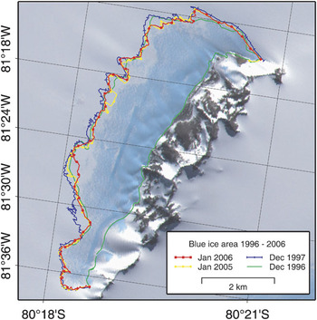
Additionally to the survey of the stake network, the perimeter of the Patriot Hills BIA was mapped during each campaign (Fig. 8). For that purpose, the outermost occurrence of bare ice was surveyed kinematically by GPS using a snowmobile. The interpretation of the snow-ice limit is in many places subjective and depends on the snow patch distribution at the time of measurement. The limit between blue ice and rock was assumed to be stable and deduced from a combination of 1996 and 1997 measurements.
Edge of blue ice area in 1996, 1997, 2005 and 2006. The ice runway appears as a darker straight line in the ASTER image.
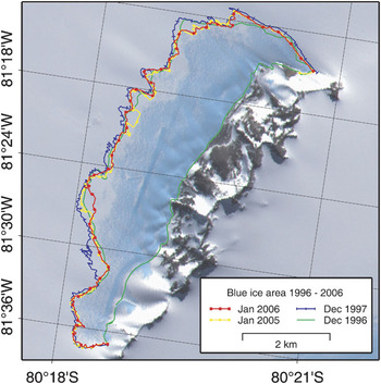
In general, there is no consistent shift of the edge of the blue ice. Only on the eastern side a segment of a length of about 600 m shifted consistently by 200–300 m towards the mountains between 1996/1997 and 2005/2006. It is particularly noticeable that the 1997 limit differs substantially from the rest and exhibits a larger snow-free surface.
Comparing the area covered by blue ice gives a more integrated measure of change. The measurements of 1996 had to be complemented on a 2 km long stretch by observations of 1997, because the perimeter is not complete due to missing data. This concerns about 7% of the BIA in the western part where the perimeter of each year coincides quite well and therefore the effect on the comparison should be minor. The resulting areas are 12.59 km2 for 1996, 13.83 km2 for 1997, 12.60 km2 for 2005, and 12.62 km2 for 2006, respectively. This supports the idea of 1997 being an extraordinary year with positive temperatures at Patriot Hills (Carrasco et al. Reference Carrasco, Casassa and Rivera2000, Casassa et al. Reference Casassa, Rivera, Acuña, Brecher and Lange2004), associated melting on the blue ice, with higher ablation rates and exceptional surface lowering.
In 2006 three stakes on the BIA originally observed by GPS in 1996 still existed and the surface elevation at these locations could be remeasured statically. They exhibit an elevation increase between 0.099 m and 0.245 m resulting in rates of up to 0.027 m a-1 ± 0.005 m a-1.
The blue ice runway (straight dark line in the ASTER image in Fig. 8) was surveyed twice, in December 1996 and January 2005, by a kinematic GPS grid. The significance of any elevation changes of this part of the blue ice can be questioned as there are man-made changes to maintain the runway free of snow. One can argue that the clearance of snow by a snowblower only accelerates the effect of the katabatic winds, which keeps the blue ice snow-free, but in fact the machines also level the ice, abrading the rippled surface. However, the direct comparison of points closer than 15 m in both surveys shows a mean height increase of 0.048 m a-1 in eight years in accordance with the results of the entire Horseshoe Valley profile.
Discussion and conclusions
Based on the field data collected between 1996 and 2006, there are two estimates of the mass balance state of Horseshoe Valley. The glaciological method comparing input (accumulation and inflow through the ice cliffs) and outflow of the valley through the surveyed profile gives no indication of a significant mass change, but with large error margins due to the lack of measurements of the ice cliff contribution. The most reliable estimation of the mean surface height change at the mouth of Horseshoe Valley using the geodetic method is an elevation increase of 0.04 m a-1 ± 0.002 m a-1 over the nine year period between November 1996 and January 2006, which is the result of comparing the elevations of 80 stake positions. Now we will discuss possible effects that contribute to this surface height change.
In general, an elevation change of the ice surface can be interpreted as a combination of a change of the height of the underlying bedrock and a change in ice thickness. The first effect can be caused by glacial isostatic adjustment and amounts to an uplift of a few millimetres per annum (Ivins & James Reference Ivins and James2005), but it is not relevant in this study because height changes were measured relative to a nearby site on bedrock that is influenced in a similar way. The second effect of changes in the ice thickness, the focus of this study, can be attributed either to changes in surface accumulation and ablation, to a difference in ice flux, or - on a snow surface - to a variation in the density of the snow due to variable firn compaction (Paterson Reference Paterson1994). For the latter effect, Zwally et al. (Reference Zwally, Giovinetto, Li, Cornejo, Beckley, Brenner, Saba and Yi2005) compute firn compaction rates based on a temperature-driven firn compaction model and give a surface lowering up to 0.01 m a-1 for the region of Patriot Hills due to climate warming. Thus the main components that could explain the surface height increase at Patriot Hills are changes in surface accumulation and ablation, and/or a change in ice flux. Due to lack of long-term data the exact causes of the surface increase cannot be determined. Considering firn compaction, the best estimation of a thickness change at Horseshoe Valley is 0.05 m a-1 ± 0.002 m a-1. Assuming the determined thickness change on the profile to be representative for the whole valley, we estimate the volume increase to be 0.054 km3 a-1 ± 0.0054 km3 a-1. Due to the lack of knowledge of the reason of thickening and whether the gained volume consists of snow or of ice, converting the volume change into a mass leaves a huge range of 20 Mt a-1 and 47 Mt a-1 depending on the density applied.
To evaluate our result we go back to the determined elevation change rate and compare it with other mass balance analyses. There are several large-scale studies about the change in ice sheet surface elevation based on satellite radar altimetry (Zwally et al. Reference Zwally, Giovinetto, Li, Cornejo, Beckley, Brenner, Saba and Yi2005, Davis et al. Reference Davis, Li, McConnell, Frey and Hanna2005, Wingham et al. Reference Wingham, Shepherd, Muir and Marshall2006), or Synthetic Aperture Radar Interferometry (Joughin & Bamber Reference Joughin and Bamber2005). These studies indicate a surface height increase between 0.011 m a-1 and 0.024 m a-1 in the region of Horseshoe Valley with errors in the range of few millimetres up to 0.015 m a-1.
Whereas these results are based on large-scale investigations that integrate over a certain area and therefore level out spatial heterogeneities, here we look at a spot measurement in a mountainous region where local effects could predominate. Nevertheless, the statistics approximately agree, suggesting a positive but small elevation change.
The BIA at Patriot Hills does not show any significant changes in areal extent. The few data available suggest a slight thickening of the blue ice. This contrasts results of some BIAs near the coast that seem to undergo a thinning (e.g. Horwath et al. Reference Horwath, Dietrich, Baessler, Nixdorf, Steinhage, Fritzsche, Damm and Reitmayr2006).
Finally, new radar data show that the ice at the centre of Horseshoe Valley is considerably thicker than previously estimated with ice thicknesses of more than 2200 m.
Acknowledgements
We thank Antarctic Logistics and Expedition and the Chilean Army for logistic support in the 2004, 2006, and 2007 seasons. Ice thickness measurements in 2007 were conducted by D. Ulloa and analysed by R. Zamora. The figures were produced using the Generic Mapping Tools GMT (Wessel & Smith Reference Wessel and Smith1998). ASTER satellite images were obtained from the project Global Land Ice Measurements from Space (GLIMS). This work was supported by a fellowship within the Postdoctoral Programme of the German Academic Exchange Service (DAAD). The Centro de Estudios Científicos (CECS) is funded by the Chilean Government through the Millennium Science Initiative and the Centers of Excellence Base Financing Program of CONICYT. CECS is also supported by a group of private companies which at present includes Antofagasta Minerals, Arauco, Empresas CMPC, Indura, Naviera Ultragas and Telefónica del Sur. We thank Tom Neumann and an anonymous reviewer for their comments that helped improve the paper.