
1. Introduction
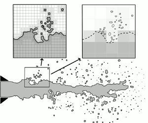
Two-phase flows encompass a wide range of physical phenomena, presenting dynamics involving a large spectrum of scales (Scardovelli & Zaleski Reference Scardovelli and Zaleski1999; Shinjo & Umemura Reference Shinjo and Umemura2010; Tomar et al. Reference Tomar, Fuster, Zaleski and Popinet2010; Dumouchel et al. Reference Dumouchel, Blaisot, Bouche, Ménard and Vu2015; Cordesse et al. Reference Cordesse, Remigi, Duret, Murrone, Ménard, Demoulin and Massot2020b; Estivalezes et al. Reference Estivalezes2022; Sakano et al. Reference Sakano, Nambu, Mizobuchi and Sato2022). We identify, in particular, two different regimes based on the topology/geometry of the fluid interfaces (Ishii & Hibiki Reference Ishii and Hibiki1975): separated-phases flows, where the material interface is described at the bulk fluid scale (hereafter called large scale), and disperse flows, characterised by the presence of disperse phases within a carrier fluid, resulting in interfaces with significantly smaller scales (hereafter called small scale).
Simulating such flows is crucial for many industrial processes such as combustion chambers where liquid fuel is injected at high velocity and pressure forming a cloud of liquid droplets further away from the nozzle or nucleate boiling in nuclear reactors (Jamet et al. Reference Jamet, Lebaigue, Morel and Arcen2010; Providakis et al. Reference Providakis, Zimmer, Scouflaire and Ducruix2012; Fiorina et al. Reference Fiorina2016). Unfortunately, direct numerical simulation (DNS) capturing the smallest interfacial variations is currently limited to academic configurations and impractical in industrial contexts. We address these challenges through the development of new modelling approaches.
One such approach, known as sub-scale modelling, consists of modelling the sub-scale phenomena directly at the bulk scale. Various approaches have been proposed for both separated and disperse flow regimes, such as two-fluid systems of equations (Baer & Nunziato Reference Baer and Nunziato1986; Raviart & Sainsaulieu Reference Raviart and Sainsaulieu1995; Saurel, Chinnayya & Carmouze Reference Saurel, Chinnayya and Carmouze2017). However, they often offer limited information about the interfacial structures and are only adapted to one of the two regimes. Several works aim at coupling both regimes (Devassy, Habchi & Daniel Reference Devassy, Habchi and Daniel2015; Le Touze et al. Reference Le Touze, Dorey, Rutard and Murrone2020) and sometimes include other modelling approaches such as Lagrangian models (Lebas et al. Reference Lebas, Menard, Beau, Berlemont and Demoulin2009). In the mixed regime zone, when the separated regime transitions to the disperse regime, the coupling processes involve very different descriptions, variables as well as a series of coupling parameters. They have to be tuned depending on the configuration of interest, which prevents the possibility of predictive simulations. The present work aims at providing a unified formalism that naturally degenerates towards separated and disperse flow models, and that can handle the mixed zone where both large and small scales are present.
This contribution takes advantage of a new versatile framework to derive unified two-scale two-phase models (Loison et al. Reference Loison, Kokh, Pichard and Massot2024) based on Hamilton's stationary action principle (SAP) (Herivel Reference Herivel1955; Serrin Reference Serrin1959; Salmon Reference Salmon1983; Bedford Reference Bedford1985; Truskinovsky Reference Truskinovsky1991; Gavrilyuk, Gouin & Perepechko Reference Gavrilyuk, Gouin and Perepechko1998; Gouin & Gavrilyuk Reference Gouin and Gavrilyuk1999; Gavrilyuk & Saurel Reference Gavrilyuk and Saurel2002; Berdichevsky Reference Berdichevsky2009; Drui et al. Reference Drui, Larat, Kokh and Massot2019; Cordesse et al. Reference Cordesse, Di Battista, Chevalier, Matuszewski, Ménard, Kokh and Massot2020a; Gouin Reference Gouin2020) and the second principle of thermodynamics. The originality of the approach relies on the models’ ability to account for the presence of both separated and disperse regimes at the same time. This is made possible by considering an artificial mixture in which small-scale and large-scale interfaces coexist within the same physical domain. The length-scale threshold that separates the large-scale dynamics of the bulk phase from the dynamics of the small-scale depends on the physics and is not discussed in this work. By employing Hamilton's SAP and an evolution equation for the mathematical entropy of the model, we can obtain a dissipative system that captures the behaviour of this multiphase medium and provides a good mathematical framework to analyse such models.
The main contribution of this work lies in the ability to plug into this two-scale framework a hierarchy of small-scale models for the disperse flow regime coupled to the large scale via a liquid mass transfer. We notably extend the geometric method of moments (GeoMOM) of Essadki et al. (Reference Essadki, Drui, de Chaisemartin, Larat, Ménard and Massot2019) which connects geometric description of the small-scale interfaces (Pope Reference Pope1988; Drew Reference Drew1990) with the statistics of a spray of droplets (Massot et al. Reference Massot, Kumar, Gomez and Smooke1998; Laurent & Massot Reference Laurent and Massot2001; Fox & Marchisio Reference Fox and Marchisio2007; Massot Reference Massot2007). We propose, in particular, a reduced-order moment model for the dynamics of the small-scale inclusions that degenerates toward an existing moment models for the disperse regime in the static minimal surface configuration of spherical polydisperse droplets (Kah et al. Reference Kah, Emre, Tran, de Chaisemartin, Jay, Laurent and Massot2015; Essadki et al. Reference Essadki, de Chaisemartin, Laurent and Massot2018), but can also handle the dynamic case of incompressible oscillation of droplets at the kinetic level following O'Rourke & Amsden (Reference O'Rourke and Amsden1987) to model deformed inclusions. The key ingredient is the proper choice of variables, which are moments of this kinetic description, but can also be identified as surface-averaged geometric quantities related to the interface dynamics independently of the flow topology. By including an inter-scale transfer, this paves the way to the modelling of the mixed zone, where the shape of droplets and ligaments depart significantly from a spherical form.
Lastly, we demonstrate the compatibility of the obtained small-scale models with several existing models from the literature that describe the evolution of the interfacial area density in the flow. It offers a new way on selecting the adequate variables for interface dynamics description and reaches interesting closures, usually out of reach, for the interfacial area density equation.
The definition of the two-scale mixture and the derivation of its dynamics with Hamilton's SAP is recalled in § 2 following Loison et al. (Reference Loison, Kokh, Pichard and Massot2024). Then, the small-scale modelling of polydisperse sprays with GeoMOM is proposed in § 3. We pursue with an extension of the polydisperse model of spherical droplets into a spray of oscillating droplets in § 4. An inter-scale mass transfer coupling the resulting hierarchy of two-scale models is then defined in § 5. Finally, the dynamics of interface area density of these models is discussed and compared with models of the literature in § 6.
2. Two-scale two-phase model for both separated and disperse regimes
We model a mixture composed of large-scale liquid and gaseous phases in a separated regime and a small-scale liquid phase, the dynamics of which is characterised by a length scale yet to be determined. The regime of the small-scale phase is not prescribed here, but it is eventually described by a disperse regime model. This section recalls the two-scale model obtained in Loison et al. (Reference Loison, Kokh, Pichard and Massot2024) which proposes a framework to account for the presence of both large-scale and small-scale phases at the same location. The interested reader is referred to the discussions therein for more details.
2.1. Two-scale modelling assumptions
We propose successive sets of assumptions. First, regarding the fluid dynamics:
 \begin{align}
{(a)}\ &\textrm{all phases have the same mean velocity;} \end{align}
 \begin{align}
{(b)}\ &\textrm{the small-scale velocity fluctuations and capillarity forces } \nonumber\\
& \textrm{are modelled by a small-scale energy term}; \end{align}
 \begin{align} {(c)}\ & \textrm{the small-scale liquid phase is incompressible.} \end{align}
Following hypotheses (H1a) and (H1b), we account for velocities that naturally appear at small scale (e.g. droplets’ drag in the disperse regime) only through the advection of a local small-scale energy for the sake of clarity of the exposition of the new ideas of the paper. Potential extensions are discussed in the conclusion. The incompressibility of the small-scale is discussed in Appendix A to justify (H1c). It affects the physics at two levels. The first level pertains to sound propagation that is cancelled at the small scale. It is especially relevant in the disperse regime where no sound can propagate from one inclusion to another as underlined in Saurel et al. (Reference Saurel, Chinnayya and Carmouze2017). The second level is related to the volume occupation of the disperse phase and the evolution of its volume fraction.
Second, the following hypotheses are formulated solely for the sake of simplicity, but are not limiting for the models developed in the present work:
 \begin{align}
{(a)}\ &\textrm{each phase is isothermal with barotropic equations of state;} \end{align}
 \begin{align}
{(b)}\ &\textrm{large-scale capillarity effects are not modelled;}
\end{align}
 \begin{align}
{(c)}\ &\textrm{no mass exchanges between the phases are taken into account;} \end{align}
 \begin{align}
{(d)}\ &\textrm{body forces are neglected.} \end{align}
Let us remark that (H1a) and (H2a) correspond to the thermal and kinematic equilibria as studied in Chanteperdrix, Villedieu & Vila (Reference Chanteperdrix, Villedieu and Vila2002), Caro et al. (Reference Caro, Coquel, Jamet and Kokh2005) and Drui et al. (Reference Drui, Larat, Kokh and Massot2019). The effects neglected by (H2a), (H2b) and (H2c) have been studied, for instance, in Perigaud & Saurel (Reference Perigaud and Saurel2005), Gaillard (Reference Gaillard2015), Schmidmayer et al. (Reference Schmidmayer, Petitpas, Daniel, Favrie and Gavrilyuk2017), Cordesse (Reference Cordesse2020), Loison et al. (Reference Loison, Kokh, Pichard and Massot2024), Caro et al. (Reference Caro, Coquel, Jamet and Kokh2005) and Pelanti (Reference Pelanti2022). The model can be extended to include these effects, but they are not necessary for the two-scale modelling framework at stake in this work. The particular modelling of mass transfer between the large scale and the small scale is not considered in this section but accounted in § 5.
We denote with the subscript  $k=1$ the liquid and
 $k=2$ the gaseous phase. An additional superscript
 $d$ identifies the small-scale liquid phase, where the letter
 $d$ stands for ‘droplets’ or ‘disperse’ liquid phase. Following (H2a), each large-scale fluid
 $k=1,2$ is equipped with a barotropic equation of state of the form
 $\rho _k \mapsto e_k (\rho _k)$, where
 $\rho _k$ and
 $e_k$ are the density and the barotropic potential of the phase
 $k=1,2$. Denoting
 $({\cdot })\mapsto ({\cdot })'$ the derivative with respect to the density, the pressure
 $p_k$ of the large-scale phase
 $k=1,2$ is then defined by
 $p_k = \rho _k^2 e_k'(\rho _k)$. We assume that
 $p_k'(\rho _k)>0$ so that the sound speed
 $c_k$ associated with the phase
 $k=1,2$ is
 $c_k=\sqrt {p_k'(\rho _k)}$. With
 $\alpha _k$ the volume fraction of the phase
 $k=1,2,1^d$, we consider a two-scale mixture such that it obeys the volume constraint
 \begin{equation} \alpha_1 + \alpha_2 + \alpha_1^d = 1, \end{equation}
and its density  $\rho$ is obtained from the effective phase densities
 $m_k := \alpha _k\rho _k$,
 \begin{equation} m_1 + m_2 + m_1^d = \rho. \end{equation}
Following Loison et al. (Reference Loison, Kokh, Pichard and Massot2024), we introduce the large-scale volume fractions defined by
 \begin{equation} \bar{\alpha}_k:=\frac{\alpha_k}{1-\alpha_1^d} \quad \textrm{for}\ k=1,2, \end{equation}
extending the usual definition at the large-scale perspective such that
 \begin{equation} \bar{\alpha}_1 + \bar{\alpha}_2=1. \end{equation}
We denote by  $Y_k$ the mass fraction such that the specific barotropic potential
 $e$ of the two-phase material is defined by
 \begin{equation} e = Y_1 e_1(\rho_1) + Y_2 e_2(\rho_2) + Y_1^d e_1(\rho_1^d). \end{equation}
Under assumptions (H1a) and (H1b), there is a unique velocity  $\boldsymbol {u}$ describing the mixture
 \begin{equation} \boldsymbol{u}:= \boldsymbol{u}_1 = \boldsymbol{u}_2 = \boldsymbol{u}_1^d. \end{equation}
Then, (H2c) provides the mass conservation of each phase
 \begin{equation} \partial_t m_k + \boldsymbol{\nabla} \boldsymbol{\cdot} (m_k \boldsymbol{u}) = 0 \quad \textrm{for} \ k=1,2,1^d. \end{equation}
Summing these equations provides the total mass conservation equation
 \begin{equation} \partial_t \rho + \boldsymbol{\nabla}_{\boldsymbol{x}}\boldsymbol{\cdot} (\rho \boldsymbol{u})=0. \end{equation}
Denoting  $D_t({\cdot })=\partial _t({\cdot }) + \boldsymbol {u} \boldsymbol {\cdot } \boldsymbol {\nabla } ({\cdot })$ the material time derivative, the incompressibility of the small-scale liquid phase (H1c) reads
 \begin{equation} D_t \rho_1^d = 0. \end{equation}
Then liquid volume fraction of the small scale is conserved
 \begin{equation} \partial_t \alpha_1^d + \boldsymbol{\nabla} \boldsymbol{\cdot} (\alpha_1^d \boldsymbol{u}) = 0. \end{equation}
The small-scale energy density accounting for both capillarity energy and kinetic energy of velocity fluctuations is advected at the mixture averaged velocity
 \begin{equation} D_t \zeta = 0. \end{equation}
2.2. Conservative motion with Hamilton's SAP
The equation of the two-scale fluid mixture's motion is derived similarly as Gavrilyuk & Gouin (Reference Gavrilyuk and Gouin1999) and Drui et al. (Reference Drui, Larat, Kokh and Massot2019) by using Hamilton's SAP. We set the kinetic and potential energies of the phase  $k$ as
 \begin{equation} E_k^{kin}:= \tfrac{1}{2}m_k \boldsymbol{u}^2, \quad E_k^{pot}:= m_k e_k\left(\frac{m_k}{\alpha_k}\right), \end{equation}
and the mixture kinetic and potential energies are  $\sum _k E_k^{kin}$ and
 $\sum _k E_k^{pot}$. This enables the definition of the Lagrangian energy
 ${\mathcal {L}}_k=E_k^{kin}-E_k^{pot}$ of the phases
 $k=1,2$,
 ${\mathcal {L}}_1^d=E_1^{d,kin}-E_1^{d,pot}-m_1^d\zeta$ and a mixture Lagrangian energy
 ${\mathcal {L}}=\sum _k{\mathcal {L}}_k$. Capillarity energy at large scale is purposely not modelled for simplifying purposes (see (H2b)) and no particular flow regime is assumed for now at small scale. These effects are considered later in § 3, where we refine the small-scale model. Thereby, the Lagrangian associated with our system reads
 \begin{equation} {\mathcal{L}} = {\mathcal{L}}_1(\alpha_1, m_1, \boldsymbol{u}) +{\mathcal{L}}_2(\alpha_2, m_2, \boldsymbol{u}) +{\mathcal{L}}_1^d(m_1^d, \rho_1^d, \zeta, \boldsymbol{u}). \end{equation}
With mass conservation constraints, Hamilton's SAP leads to the following set of equations (see Appendix B for details)
 \begin{equation} \left.\begin{array}{@{}c@{}} \partial_t m_k + \boldsymbol{\nabla} \boldsymbol{\cdot} (m_k \boldsymbol{u})=0,\quad k=1,2,1^d, \\ \partial_t \alpha_1^d + \boldsymbol{\nabla} \boldsymbol{\cdot} (\alpha_1^d \boldsymbol{u})=0,\\ \partial_t \zeta + \boldsymbol{u} \boldsymbol{\cdot} \boldsymbol{\nabla} \zeta=0,\\ \partial_t (\rho \boldsymbol{u}) + \boldsymbol{\nabla} \boldsymbol{\cdot} (\rho \boldsymbol{u} \otimes \boldsymbol{u} + p \boldsymbol{\mathsf{I}})=0, \end{array}\right\} \end{equation}
where  $\boldsymbol{\mathsf{I}}$ is the identity matrix, and
 $p$ is the equilibrium pressure obtained for the mixture thermodynamic closure
 $p:=p_1=p_2$ given by the second line of (B16). This algebraic equation gives
 $\alpha _1$ and
 $p$, respectively, as the solution and the value of the equilibrium for given values of
 $m_1$,
 $m_2$ and
 $\alpha _1^d$. System (2.14) also admits a supplementary conservation equation
 \begin{equation} \partial_t {\mathcal{H}} + \boldsymbol{\nabla} \boldsymbol{\cdot}(({\mathcal{H}}+p)\boldsymbol{u})=0, \end{equation}
where the total energy  ${\mathcal {H}} = \rho \Vert \boldsymbol {u}\Vert ^2 - {\mathcal {L}}$ is a mathematical entropy (Godlewski & Raviart Reference Godlewski and Raviart1991) for (2.14). The mathematical entropy of the system is studied as the isothermal limit of the Euler–Fourier model in Serre (Reference Serre2010). It is shown to be convex and linked to the physical entropy of the mixture
 $s$ with
 ${\mathcal {H}}=\rho (\varepsilon -Ts) + \tfrac {1}{2}\rho \Vert \boldsymbol {u}\Vert ^2$ where
 $\varepsilon = e + Ts$ and
 $T$ are the internal energy and the temperature of the mixture, respectively.
Remark that  $\alpha _1$ is not a variable of the set of conservation laws (2.14), but its effective dynamics for smooth solution can be written explicitly by applying the material time derivative to the algebraic equation
 $p_1(m_1/\alpha _1)=p_2(m_2/(1-\alpha _1-\alpha _1^d))$, and reads
 \begin{align} D_t \alpha_1 =
\varLambda
\boldsymbol{\nabla}\boldsymbol{\cdot}\boldsymbol{u} \quad
\textrm{with} \ \varLambda =
\alpha_1(1-\alpha_1)\tfrac{\rho_2
c_2^2\,-\,\rho_1c_1^2}{\alpha_1\rho_2c_2^2\,+\,(1-\alpha_1)\rho_1c_1^2}+\alpha_1^d
\tfrac{\alpha_1\rho_2c_2^2}{\alpha_1\rho_2c_2^2\,+\,(1\,-\,\alpha_1)\rho_1c_1^2}.
\end{align}
Moreover, system (2.14) is shown hyperbolic with a mixture's velocity  $c_W^d:=c_W/(1-\alpha _1^d)$ where
 $c_W$ is the Wood sound velocity such that
 $(c_W^2)^{-1}=\rho (\alpha _1/(\rho _1c_1^2)+\alpha _2/(\rho _2c_2^2))$. This extends, in particular, the three-equation model proposed by Chanteperdrix et al. (Reference Chanteperdrix, Villedieu and Vila2002), which is recovered when
 $\alpha _1^d\rightarrow 0$.
Remark also that the small-scale specific energy  $\zeta$ is chosen to be modelled here as a passively advected quantity. Therefore, it does not affect the dynamics of the two-scale mixture in absence of inter-scale mass transfer which is further modelled in § 5. The modelling of the effect of small-scale velocity fluctuations on large-scale dynamics, possibly via pressure contributions, is however out of the scope of this work. Because of this temporary passive role and for clarity purposes, this small-scale energy is removed from the modelling up to § 5.
2.3. Dissipative dynamics
Now that we have set the conservative structure of the model with Hamilton's SAP, we add dissipative processes to the model. We propose here to model both a pressure disequilibrium between the two large-scale phases as it is characteristic of two-phase flow models as in the model of Baer & Nunziato (Reference Baer and Nunziato1986) and fluid viscosity.
First, the pressure disequilibrium can encompass several physical phenomena with different timescales [e.g. bubbly flows (Drui et al. Reference Drui, Larat, Kokh and Massot2019) and stochastic thermodynamic relaxation (Perrier & Gutiérrez Reference Perrier and Gutiérrez2021)]. Let us mention that the limit of instantaneous relaxation can also be used to build a numerical scheme that solves the pressure equilibrium of (2.14) (Chanteperdrix et al. Reference Chanteperdrix, Villedieu and Vila2002).
In order to make this pressure relaxation a large-scale process that acts on each large-scale phase symmetrically, we define the large-scale volume fractions
 \begin{equation} \bar{\alpha}_k:=\frac{\alpha_k}{1-\alpha_1^d} \quad \textrm{for}\ k=1,2, \end{equation}
such that for  $\alpha _1^d< 1$,
 \begin{equation} \alpha_1+\alpha_2+\alpha_1^d=1 \ \iff\ \bar{\alpha}_1 + \bar{\alpha}_2=1. \end{equation}
Then, we relax the pressure equilibrium of (2.14) into
 \begin{equation} D_t \bar{\alpha}_1 = \frac{p_1-p_2}{\epsilon}, \end{equation}
where  $\epsilon >0$ has the dimension of a dynamic viscosity. Since the pressure is no longer unique with this pressure relaxation, the momentum equation can be expressed as follows:
 \begin{equation} \partial_t (\rho \boldsymbol{u}) + \boldsymbol{\nabla} \boldsymbol{\cdot} (\rho \boldsymbol{u} \otimes \boldsymbol{u}+\bar{p} \boldsymbol{\mathsf{I}})=0, \end{equation}
where  $\bar {p}$ is chosen to provide a signed dissipation of
 ${\mathcal {H}}$. Following Appendix B,
 \begin{align} \varsigma&:= \partial_t {\mathcal{H}} +\boldsymbol{\nabla}\boldsymbol{\cdot}(({\mathcal{H}}+\bar{p}) \boldsymbol{u}) \nonumber\\ &= (\kern0.7pt \bar{p}-\alpha_1p_1-(\alpha_2+\alpha_1^d)p_2)\boldsymbol{\nabla}\boldsymbol{\cdot}\boldsymbol{u} - (p_1-p_2) D_t \alpha_1 \nonumber\\ &= (\kern0.7pt \bar{p}-\bar{\alpha}_1p_1-\bar{\alpha}_2p_2)\boldsymbol{\nabla}\boldsymbol{\cdot}\boldsymbol{u} - \epsilon (1-\alpha_1^d) (D_t\bar{\alpha}_1)^2. \end{align}
Therefore, choosing  $\bar {p}:=\bar {\alpha }_1p_1 + \bar {\alpha }_2p_2$ gives a signed mathematical entropy production
 $\varsigma \le 0$ and the relaxed model reads
 \begin{equation} \left.\begin{array}{@{}c@{}} \partial_t m_k +\boldsymbol{\nabla} \boldsymbol{\cdot} (m_k \boldsymbol{u})=0\quad \textrm{for} \ k=1,2,1^d, \\ \partial_t \alpha_1^d + \boldsymbol{\nabla} \boldsymbol{\cdot} (\alpha_1^d \boldsymbol{u})=0,\\ \partial_t (\rho \boldsymbol{u}) + \boldsymbol{\nabla} \boldsymbol{\cdot} (\rho \boldsymbol{u} \otimes \boldsymbol{u}+ \bar{p}\boldsymbol{\mathsf{I}})=0,\\ D_t \bar{\alpha}_1= \epsilon^{{-}1}(p_1-p_2). \end{array}\right\} \end{equation}
The model (2.22) is obtained for the specific dissipative process (2.19) that gives a relaxed model for (2.14). It is also shown hyperbolic with a mixture's velocity  $c_F^d:=c_F/(1-\alpha _1^d)$ where
 $c_F$ is the frozen sound velocity such that
 $c_F^2 = Y_1c_1^2+Y_2c_2^2$. The reader is referred to Loison et al. (Reference Loison, Kokh, Pichard and Massot2024) for a more thorough discussion on the pair of two-scale systems (2.14) and (2.22).
Second, the fluid viscosity in the context of a two-phase diffuse interface model with one velocity can be modelled with a Stokes source term on the momentum equation
 \begin{equation} \partial_t (\rho \boldsymbol{u}) + \boldsymbol{\nabla} \boldsymbol{\cdot} (\rho \boldsymbol{u} \otimes \boldsymbol{u}+ \bar{p}\boldsymbol{\mathsf{I}})= \boldsymbol{\nabla}\boldsymbol{\cdot}\boldsymbol{T}_{stokes}, \end{equation}
where  $\boldsymbol {T}_{stokes}:=\mu (\boldsymbol {\nabla } \boldsymbol {u} + (\boldsymbol {\nabla } \boldsymbol {u})^\textrm {T}) + \lambda (\boldsymbol {\nabla }\boldsymbol {\cdot }\boldsymbol {u})\boldsymbol {I}$ is the viscous stress,
 $\mu$ the dynamic viscosity and
 $\lambda$ the second viscosity with
 $\lambda + \frac {2}{3}\mu \ge 0$. After some calculations, this additional term modifies the mathematical entropy production (2.21) to yield
 \begin{align} &\partial_t {\mathcal{H}} +\boldsymbol{\nabla}\boldsymbol{\cdot}(({\mathcal{H}}+\bar{p}) \boldsymbol{u}-\boldsymbol{T}_{stokes}\boldsymbol{\cdot} \boldsymbol{u})\nonumber\\ &\quad ={-} \epsilon (1-\alpha_1^d) (D_t\bar{\alpha}_1)^2 - \!\left( 2\mu \left(\frac{\boldsymbol{\nabla}\boldsymbol{u} + (\boldsymbol{\nabla}\boldsymbol{u})^T}{2}-\frac{1}{3}(\boldsymbol{\nabla}\boldsymbol{\cdot}\boldsymbol{u})\right)^2 + \left(\lambda + \frac{2}{3}\mu\right)(\boldsymbol{\nabla}\boldsymbol{\cdot}\boldsymbol{u})^2 \right)\!. \end{align}
The right-hand side is negatively signed and thus provides a dissipative term to the dynamics.
Including these two viscosity terms, a dimensionless analysis of the dissipative system is proposed in Appendix C. In the remainder of this paper, such viscous terms are neglected for readability purposes, but their absence could also correspond to regimes with high fluid velocities.
We remark that other dissipative processes could have been considered, but are not modelled here, such as drag for two-velocity models (Saurel et al. Reference Saurel, Chinnayya and Carmouze2017; Gavrilyuk Reference Gavrilyuk2020) or turbulent dissipation (Saurel, Gavrilyuk & Renaud Reference Saurel, Gavrilyuk and Renaud2003).
3. Small-scale modelling consistent with polydisperse sprays of spherical droplets
We now follow two parallel goals to enrich the small-scale models of the previous section: (1) describing polydisperse sprays in the disperse regime, where the droplets are spherical, in their static minimal surface configuration; and (2) introducing geometric quantities which describe the small scale for any kind of interface in all flow regimes, thus proposing a limit model of a general interface dynamics at small scale. This modelling strategy has first been introduced for droplets in spherical shape in Essadki et al. (Reference Essadki, de Chaisemartin, Massot, Laurent, Larat and Jay2016) and will be referred to in the present contribution as GeoMOM. This strategy relies on a kinetic modelling of the small scale as a population of droplets. The resulting model is consequently coherent in the disperse regime where the kinetic approach is valid. In the mixed regime, the physics validity of the kinetic-based model is limited, but it still remains interpretable since the chosen geometric variables are showed to be defined with both a large-scale modelling of the interface and the small-scale kinetic model.
3.1. Kinetic-based model in the disperse regime
We start the modelling of the spray by assuming that:
 \begin{align}
{(a)}\ &\textrm{the small-scale phase is composed of spherical droplets;} \end{align}
 \begin{align} {(b)}\ &\textrm{the droplets do not break nor coalesce.} \end{align}
Indeed, (H1b) shows that only small velocity differences are locally allowed at the small scale, and droplets are then very close to a spherical shape. The droplets are then described by a static minimal surface, which remains spherical. The kinetic modelling of the disperse small scale relies on the number density function (NDF)  $f$ that counts the number of droplets within a small volume of the phase space around a point of the space–time domain. For generality purpose, we adopt a description for compressible inclusions whose sizes can change in time under either mass exchange or compressibility processes. Therefore, we consider the NDF
 $f(\boldsymbol {x}, t, \boldsymbol {v}, \hat {m})$ to be a distribution of velocities
 $\boldsymbol {v}$ and droplet masses
 $\hat {m}$ instead of a size parameter such as radius or surface. We also denote
 $f_{\boldsymbol {v},m}$ for compactness to underline the phase-space dependencies only. Then, the equation of evolution of the NDF expresses the conservation of the droplets in both the real and phase spaces (Williams Reference Williams1958; Marchisio & Fox Reference Marchisio and Fox2013) and reads
 \begin{equation} \partial_t\, f_{\boldsymbol{v},m} + \boldsymbol{\nabla}_{\boldsymbol{x}}\boldsymbol{\cdot}(f_{\boldsymbol{v},m} \boldsymbol{v}) + \boldsymbol{\nabla}_{\boldsymbol{v}}\boldsymbol{\cdot}(\boldsymbol{F}(\boldsymbol{v}, \hat{m})f_{\boldsymbol{v},m}) + \partial_{\hat{m}}(R_{m}(\boldsymbol{v}, \hat{m})f_{\boldsymbol{v},m})=\varGamma, \end{equation}
where  $\boldsymbol {F}$ and
 $R_{m}$ are unclosed rates of change of the velocity and the mass corresponding to body forces and mass transfer, while
 $\varGamma =\varGamma _{bu}+\varGamma _{coal}$ accounts for source terms such as break-up and coalescence phenomena. Hypotheses (H3b) and (H2c) imply
 $\varGamma =0$ and
 $R_{m}=0$, respectively. Moreover, the distribution of velocities is out of the scope of this work as assumed by (H1a) (see Vié et al. Reference Vié, Laurent and Massot2013 for an Eulerian model coupling the effects of size and velocity distributions). Therefore, we discard the velocity dependency by considering
 $n_m = \int _{\boldsymbol {v}} f_{\boldsymbol {v}, m} \,\textrm {d}\boldsymbol {v}$, the mass-based NDF in the limit of a vanishing Stokes number
 $St \rightarrow 0$, i.e. when the inertial timescale of inclusions is negligible compared to the timescale of the flow. Following the works of Jabin (Reference Jabin2002) and Massot (Reference Massot2007), the dynamics of
 $n_m$ reads
 \begin{equation} \left.\begin{array}{@{}c@{}} \partial_t n_{m} + \boldsymbol{\nabla}_{\boldsymbol{x}}\boldsymbol{\cdot}(n_{m} \boldsymbol{u})=0,\\ \partial_t (n_{m}\boldsymbol{u}) + \boldsymbol{\nabla}_{\boldsymbol{x}}\boldsymbol{\cdot}(n_{m} \boldsymbol{u}\otimes\boldsymbol{u})=\boldsymbol{0}, \end{array}\right\} \end{equation}
where  $\boldsymbol {u}$ is the unique velocity of every phase as defined by (2.6).
3.2. GeoMOM: definition and application to the incompressible spray
GeoMOM aims at enriching the models (2.14)–(2.22) with quantities describing the geometry of the interface at the small scale. This method introduced in Essadki et al. (Reference Essadki, de Chaisemartin, Massot, Laurent, Larat and Jay2016, Reference Essadki, de Chaisemartin, Laurent and Massot2018, Reference Essadki, Drui, de Chaisemartin, Larat, Ménard and Massot2019) is a reduced-order moment model for the polydisperse droplet distribution where the chosen moments are geometric quantities that can be defined for any flow regime and interface topology.
First, let us define those quantities. We consider a surface  ${\mathcal {S}}$ defined by mapping a set
 ${\mathcal {U}}\subset \mathbb {R}^2$ onto
 ${\mathcal {S}}\subset \mathbb {R}^3$ such that we denote by
 $A(u,v)\,\textrm {d}u\,\textrm {d}v$ the infinitesimal surface element over
 ${\mathcal {S}}$. Then, the surface area and a surface-average operator are defined on
 ${\mathcal {S}}$ by
 \begin{equation} S:= \int_{{\mathcal{U}}} A(u,v)\,{\rm d}u,{\rm d}v, \quad \langle {\cdot}\rangle:=\frac{1}{S}\int_{{\mathcal{U}}}({\cdot}) A(u,v)\,{\rm d}u\,{\rm d}v. \end{equation}
Considering the surface of the droplets in the two-scale mixture as described in § 2, the sum of their areas defines the small-scale interface area density  $\varSigma$. Thanks to (3.3), one can also define surface-average Gauss and mean curvatures
 $\varSigma \langle G\rangle$ and
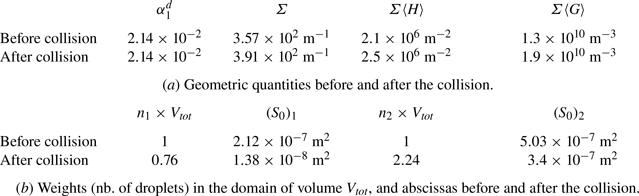
 $\varSigma \langle H\rangle$ as in Drew (Reference Drew1983) and Pope (Reference Pope1988). We use here these quantities to enhance the description of the disperse small scale, but their definitions are a priori independent of the surface geometry (see an application of these geometric quantities to the interface resulting from for the collision of two spherical droplets in Appendix D). This property is particularly convenient as it indicates that the kinetic-based model can be interpreted as a limit case for the mixed regime, and we discuss in conclusion how it allows coupling of the interface geometry between scales.
Second, we reduce the complexity of the spray dynamics, modelled by the distribution  $n_m$ given in (3.2), by introducing a finite set of moments indexed by
 ${\mathcal {I}}$
 \begin{equation} M_i^m := \int_{\hat{m}} \hat{m}^i n_m \, {\rm d}\hat{m}, \quad i\in {\mathcal{I}} \textrm{ finite }\subset\mathbb{N}. \end{equation}
These scalars retain statistical information about the NDF and their dynamics can be obtained by integrating (3.2) against the corresponding monomials,
 \begin{equation} \partial_t M_i^m + \boldsymbol{\nabla}\boldsymbol{\cdot}(M_i^m\boldsymbol{u})=0, \quad i\in{\mathcal{I}}. \end{equation}
The method of moments then gives a reduced-order model for the small-scale spray in comparison with (3.2). In general, the equations are unclosed, and a reconstruction of the NDF based on the selected moments must be provided. The selection of these moments is not obvious and is usually motivated on the basis of mathematical properties of the resulting moment model.
Finally, the specificity of GeoMOM consists in the selection of moments related to geometric quantities defined with (3.3) to construct a model interpretable even out of the disperse regime. For the spherical droplets described by  $n_m$, the local Gauss and mean curvatures on the sphere are constant and equal to
 $R^{-1}$ and
 $R^{-2}$, respectively, where
 $R=(3m/(4{\rm \pi} \rho _1^d))^{1/3}$ is the radius of the sphere of density
 $\rho _1^d$ and mass
 $m$. Therefore, considering a population of spherical droplets, we express the geometric quantities
 $\varSigma$,
 $\varSigma \langle G\rangle$ and
 $\varSigma \langle H\rangle$ as moments of the distribution
 $n_m$
 $$\begin{gather} \varSigma\langle G\rangle = \int_{\hat{m}} 4{\rm \pi} n_m \, {\rm d}\hat{m}=4{\rm \pi} M^m_0, \end{gather}$$
 $$\begin{gather}\varSigma\langle H\rangle = \int_{\hat{m}} 4{\rm \pi} \left(\frac{3}{4{\rm \pi} \rho_1}\right)^{1/3} \hat{m}^{1/3} n_m \, {\rm d}\hat{m}=4{\rm \pi} \left(\frac{3}{4{\rm \pi} \rho_1^d}\right)^{1/3} M^m_{1/3}, \end{gather}$$
 $$\begin{gather}\varSigma = \int_{\hat{m}} 4{\rm \pi} \left(\frac{3}{4{\rm \pi} \rho_1^d}\right)^{2/3} \hat{m}^{2/3} n_m \, {\rm d}\hat{m}=4{\rm \pi} \left(\frac{3}{4{\rm \pi} \rho_1^d}\right)^{2/3} M^m_{2/3}. \end{gather}$$
Remark the special role of  $\varSigma \langle G\rangle$ proportional to the zeroth-order moment of
 $n_m$. This results from the Gauss–Bonnet theorem (Kreyszig Reference Kreyszig1991), which indicates a geometric invariant
 $S\tilde {G}=4{\rm \pi}$ for continuous deformations of the sphere, where
 $\widetilde {({\cdot })}$ denotes the surface average as (3.3) applied to a unique droplet. It is also shown in Essadki et al. (Reference Essadki, Drui, de Chaisemartin, Larat, Ménard and Massot2019) that such an invariant enables to write the dynamics of geometric quantities
 $\varSigma$,
 $\varSigma \langle {\cdot }\rangle$ independently of the flow regime. Furthermore, the small-scale volume fraction is not surface-related in general, but in the specific case of spherical droplets, it is also linked to a moment of
 $n_m$ with
 \begin{equation} \alpha_1^d=\int_{\hat{m}} \frac{1}{\rho_1^d} \hat{m} n_{m} \, {\rm d}\hat{m} = \frac{1}{\rho_1^d} M^m_1. \end{equation}
From (3.6) and (3.7), we select  ${\mathcal {I}}=\{0,1/3,2/3,1\}$ in (3.5) to obtain the dynamics of the geometric quantities
 \begin{equation} \left.\begin{array}{@{}c@{}} \partial_t (\varSigma\langle G\rangle ) + \boldsymbol{\nabla} \boldsymbol{\cdot} (\varSigma\langle G\rangle \boldsymbol{u})=0,\\ \partial_t ((\rho_1^d)^{1/3}\varSigma\langle H\rangle ) + \boldsymbol{\nabla} \boldsymbol{\cdot} ((\rho_1^d)^{1/3} \varSigma\langle H\rangle \boldsymbol{u})=0,\\ \partial_t ((\rho_1^d)^{2/3}\varSigma) + \boldsymbol{\nabla} \boldsymbol{\cdot} ((\rho_1^d)^{2/3}\varSigma \boldsymbol{u})=0,\\ \partial_t m_1^d + \boldsymbol{\nabla} \boldsymbol{\cdot} (m_1^d \boldsymbol{u})=0. \end{array}\right\} \end{equation}
Up to here, the model has been derived for compressible spherical inclusions. We focus back on the description of a spray of droplets by assuming the incompressibility of the small scale thanks to the constraint  $D_t \rho _1^d = 0$. Then, the geometric variables are governed by
 \begin{equation} \left.\begin{array}{@{}c@{}} \partial_t (\varSigma\langle G\rangle ) + \boldsymbol{\nabla} \boldsymbol{\cdot} (\varSigma\langle G\rangle \boldsymbol{u}) = 0,\\ \partial_t (\varSigma\langle H\rangle ) + \boldsymbol{\nabla} \boldsymbol{\cdot} (\varSigma\langle H\rangle \boldsymbol{u}) = 0,\\ \partial_t \varSigma + \boldsymbol{\nabla} \boldsymbol{\cdot} (\varSigma \boldsymbol{u}) = 0,\\ \partial_t \alpha_1^d + \boldsymbol{\nabla} \boldsymbol{\cdot} (\alpha_1^d \boldsymbol{u}) = 0. \end{array}\right\} \end{equation}
System (3.9) corresponds to the system with surface-based moments of Essadki et al. (Reference Essadki, de Chaisemartin, Laurent and Massot2018) when no evaporation nor condensation is accounted for. Indeed, when the droplets are incompressible, the mass-based NDF  $n_m$ relates to the surface-based NDF
 $n_{S}$ defined by
 \begin{equation} n_S(\boldsymbol{x}, t, \hat{S}):=n_m(\boldsymbol{x}, t, \hat{m})\delta(\hat{m}-m(\hat{S})), \quad m(\hat{S})=\rho_1^d\frac{\hat{S}}{3\sqrt{4{\rm \pi}}}. \end{equation}
As  $\rho _1^d$ is a constant along the streamlines, there is no variation of surface area for the droplets and the dynamics is then driven by
 \begin{equation} \partial_t n_S + \boldsymbol{\nabla}_{\boldsymbol{x}}(n_S \boldsymbol{u})=0. \end{equation}
Again, when the droplets have the same density, the geometric quantities are also expressed through the moments  $M_i^S$ of
 $n_S$,
 \begin{equation} \varSigma\langle G\rangle = 4{\rm \pi} M^S_0, \quad \varSigma\langle H\rangle = \sqrt{4{\rm \pi}} M^S_{1/2}, \quad \varSigma = M^S_1, \quad \alpha_1^d = \frac{1}{3 \sqrt{4{\rm \pi}}} M^S_{3/2}. \end{equation}
The change of variables (3.10) only modifies the dimensions and orders of the moments. Consequently, the four initial half-integer moments can be recovered as in Essadki et al. (Reference Essadki, de Chaisemartin, Laurent and Massot2018). In the following, we stick with the surface-based moments for better comparison with the work of Essadki et al. In the end, the relations (3.12) between moments and geometric quantities provide a reduced-order model of the small-scale disperse phase (see Appendix D for an illustration of the reduced-order modelling applied to droplets resulting from the collision of two spherical droplets).
3.3. A two-scale model with a polydisperse small-scale model
The two-scale models derived in § 2 thanks to Hamilton's SAP can now be enhanced by incorporating the new geometric quantities in the Lagrangian and specifying whether these parameters are constrained by new conservation laws. We add then a small-scale capillarity energy  $\sigma \varSigma$ along with the conservation constraints given by (3.9). Let us introduce a new variable
 $z=\varSigma /m_1^d$, which is transported, that is,
 $D_t z = 0$. As the large-scale capillarity is neglected (H2b), the energies associated with the large scales of the flow are left unchanged whereas the small-scale Lagrangian
 ${\mathcal {L}}_1^d$ becomes
 \begin{equation} {\mathcal{L}}_1^d(m_1^d, \rho_1^d, z:=\varSigma/m_1^d, \boldsymbol{u}):=\tfrac{1}{2}m_1^d \vert\boldsymbol{u}\vert^2 -m_1^d e_1(\rho_1^d) -\sigma m_1^d z. \end{equation}
Eventually, the system resulting from Hamilton's SAP (see details in Appendix E) together with the constraints (3.9) yields
 \begin{equation} \left.\begin{array}{@{}c@{}} \partial_t m_k + \boldsymbol{\nabla} \boldsymbol{\cdot} (m_k \boldsymbol{u})=0,\quad k=1,2,1^d, \\ \partial_t \alpha_1^d + \boldsymbol{\nabla} \boldsymbol{\cdot} (\alpha_1^d \boldsymbol{u}) =0, \\ \partial_t \varSigma +\boldsymbol{\nabla} \boldsymbol{\cdot}(\varSigma\boldsymbol{u})=0,\\ \partial_t (\varSigma\langle G\rangle ) + \boldsymbol{\nabla} \boldsymbol{\cdot} (\varSigma\langle G\rangle \boldsymbol{u}) =0, \\ \partial_t (\varSigma\langle H\rangle ) + \boldsymbol{\nabla} \boldsymbol{\cdot}(\varSigma\langle H\rangle \boldsymbol{u})=0,\\ \partial_t (\rho \boldsymbol{u})+ \boldsymbol{\nabla} \boldsymbol{\cdot} (\rho \boldsymbol{u} \otimes \boldsymbol{u}+p\boldsymbol{\mathsf{I}})=0, \end{array}\right\} \end{equation}
with  $p:=p_1=p_2$. Let us remark that the new small-scale capillarity term in the Lagrangian does not alter momentum flux in this formulation compared to (2.14). Similarly to the previous models but with the updated definition of the Lagrangian
 ${\mathcal {L}}$, this model also admits a supplementary conservation equation
 \begin{equation} \partial_t {\mathcal{H}} + \boldsymbol{\nabla} \boldsymbol{\cdot}(({\mathcal{H}}+p)\boldsymbol{u})=0, \quad {\mathcal{H}} = \sum_k m_k \Vert\boldsymbol{u}\Vert^2 - {\mathcal{L}}. \end{equation}
Both (3.14) and its relaxed version are hyperbolic with similar structure of eigenvalues and eigenvectors.
4. Polydisperse and vibrational spray small-scale model
In the previous model, no dynamics have been associated with the geometric variables as they represent a spray of spherical droplets, that is a static minimal surface. Here, we propose to enhance this model by associating a dynamics to the droplet geometry. In the context of the small velocity differential given by (H1b), we add an oscillating motion to the droplets around their spherical shapes. Such a model is sufficiently simple to identify the associated energies while being a first step towards the modelling of break-up as proposed in O'Rourke & Amsden (Reference O'Rourke and Amsden1987) and Amsden, O'Rourke & Butler (Reference Amsden, O'Rourke and Butler1989) (see figure 1). Moreover, this model introduces with GeoMOM non-trivial dynamics for geometric quantities such as interface area density.
Sphere deformed with the second axisymmetric spherical harmonic and vibrational breakup modelled by a critical length for the smallest radius.

4.1. Kinetic-based model in the disperse regime
Let us model the spray of oscillating droplets by first discarding assumption (H3a) of spherical shapes, and rather assume:
 \begin{align}
{(a)}\ &\textrm{the droplets' internal flow is irrotational; } \end{align}
 \begin{align}
{(b)}\ &\textrm{the amplitude of the interface deformation is small; } \end{align}
 \begin{align}
{(c)}\ &\textrm{the deformed droplets are either randomly orientated or they all } \nonumber \\
& \textrm{orientate to the same privileged direction;}
\end{align}
 \begin{align}
{(d)}\ &\textrm{the droplets' interface is deformed along the second } \nonumber \\
& \textrm{axisymmetric spherical harmonic.} \end{align}
The dynamics of a droplet satisfying (H4a) and (H4b) has been studied thoroughly (Rayleigh Reference Rayleigh1879; Prosperetti Reference Prosperetti1977; Plümacher et al. Reference Plümacher, Oberlack, Wang and Smuda2020). The choice of orientation (H4c) of the deformation depends on the physics, whether it is isotropic or not, and it is not discussed here. Denote by  $\boldsymbol {r}$ the position of the droplet interface in spherical coordinates
 $(r,\theta,\phi )$ and
 $(\boldsymbol {e}_r$,
 $\boldsymbol {e}_{\theta }$,
 $\boldsymbol {e}_{\phi })$ the spherical orthonormalised basis. Following (H4d), we denote by
 $Y_2(\theta ) = \sqrt {5}/(4\sqrt {{\rm \pi} })(3\cos ^2\theta -1)$ the second axisymmetric spherical harmonic, and
 $R_0$ the radius of the non-deformed spherical droplet, such that the position can be written as
 \begin{equation} \boldsymbol{r} = (R_0 + x_2 Y_2) \boldsymbol{e}_r, \end{equation}
where  $x_2$ denotes the amplitude of the deformation. The dynamics of this motion follows the harmonic oscillation
 \begin{equation} \ddot{x}_2+\omega^2 x_2 = 0,\quad \omega^2 = 8\frac{\sigma}{\rho_1^d R_0^3}=\tilde{\omega}^2S_0^{{-}3/2}, \end{equation}
where  $\tilde {\omega }^2=(8(4{\rm \pi} )^{3/2}\sigma /\rho _1^d)$ is a constant along the streamlines. The dynamics of the droplets is then characterised by
 $(S_0,x_2,\dot {x}_2)$. For computational reasons, we introduce
 $\chi = (2/S_0)^{1/2}x_2$ which satisfies the same dynamics (4.2) as
 $x_2$. Assuming (H3b) and (H2c), the balance equation for the NDF
 $n_{\xi }$ in the phase space
 $\hat {\boldsymbol {\xi }}=(\hat {S}_0, \hat {\chi }, \hat {\dot {\chi }})$ yields
 \begin{equation} \partial_t n_{\xi}+ \boldsymbol{\nabla}_{\boldsymbol{x}} \boldsymbol{\cdot} (n_{\xi}\boldsymbol{u}) + \partial_{\hat{\chi}} (R_{\chi}n_{\xi}) + \partial_{\hat{\dot{\chi}}}(R_{\dot{\chi}}n_{\xi})=0, \end{equation}
where  $R_{\chi }$ and
 $R_{\dot {\chi }}$ are rates of change that remain to be closed. This model can be seen as the particular case satisfying (H1a)–(H2c)–(H3b)–(H2a) of the kinetic model considered by O'Rourke & Amsden (Reference O'Rourke and Amsden1987), Amsden et al. (Reference Amsden, O'Rourke and Butler1989). With the oscillator model (4.2), we close (4.3) by fixing
 $R_{\chi } = \hat {\dot {\chi }}$ and
 $R_{\hat {\dot {\chi }}} = -\tilde {\omega }^2\hat {S}_0^{-3/2}\hat {\chi }$,
 \begin{equation} \partial_t n_{\xi}+ \boldsymbol{\nabla}_{\boldsymbol{x}} \boldsymbol{\cdot} (n_{\xi}\boldsymbol{u}) + \partial_{\hat{\chi}} (\hat{\dot{\chi}} n_{\xi}) + \partial_{\hat{\dot{\chi}}}(-\tilde{\omega}^2\hat{S}_0^{{-}3/2}\hat{\chi} n_{\xi})=0. \end{equation}
4.2. Modelling a spray of asynchronously oscillating droplets
With the new PBE (4.4), GeoMOM leads to a non-trivial closure problem and the geometric quantities chosen in (3.6) and (3.7) cannot model an arbitrary distribution. With such a choice, we propose in this section to approximate the distribution with
 \begin{equation} n_{\xi}(\boldsymbol{x}, t, \hat{S}_0, \hat{\chi}, \hat{\dot{\chi}}) = n_{S_0}(\boldsymbol{x}, t, \hat{S}_0) \frac{1}{\vert{\mathcal{E}}(\hat{S}_0)\vert} \mathbb{1}_{{\mathcal{E}}(\hat{S}_0)}(\hat{\chi}, \hat{\dot{\chi}}), \end{equation}
where the amplitudes and their rates of change  $(\hat {\chi }, \hat {\dot {\chi }})$ are uniformly distributed on a compact space
 ${\mathcal {E}}\subset \mathbb {R}^2$ of area
 $\vert {\mathcal {E}}(\hat {S}_0)\vert$ that allows a maximal energy for a given droplet size
 $\hat {S}_0$. This approximation of the NDF discards situations where droplets oscillate synchronously, and consequently a macroscopic oscillation motion of the spray.
4.2.1. GeoMOM based on the classical surface-average operator
We apply GeoMOM with the same surface-average operators  $\langle {\cdot }\rangle$ and
 $\widetilde {({\cdot })}$ defined in § 3.2, and geometric quantities
 $\varSigma \langle G\rangle$,
 $\varSigma \langle H\rangle$,
 $\varSigma$,
 $\alpha _1^d$. We establish then the relations between these geometric quantities and moments of the NDF in the context of a disperse regime,
 \begin{equation} \left.\begin{array}{@{}c@{}} \displaystyle \varSigma\langle G\rangle = \int_{\hat{\boldsymbol{\xi}}} S\tilde{G} n_{\xi}\,{\rm d}\hat{\boldsymbol{\xi}}, \quad \varSigma\langle H\rangle = \int_{\hat{\boldsymbol{\xi}}} S\tilde{H} n_{\xi}\, {\rm d}\hat{\boldsymbol{\xi}}, \\[14pt] \displaystyle \varSigma = \int_{\hat{\boldsymbol{\xi}}} S n_{\xi}\, {\rm d}\hat{\boldsymbol{\xi}}, \quad \alpha_1^d = \int_{\hat{\boldsymbol{\xi}}} V n_{\xi}\, {\rm d}\hat{\boldsymbol{\xi}}. \end{array}\right\} \end{equation}
When the oscillations are small, the integrands are functions of  $\hat {\boldsymbol {\xi }}$ (see Appendix F) and write
 \begin{equation} S\tilde{G}=4{\rm \pi}, \quad S\tilde{H} - S_0\tilde{H}_0 = \sqrt{4{\rm \pi}} S_0^{1/2}\chi^2, \quad V = \frac{1}{3\sqrt{4{\rm \pi}}} S_0^{3/2}, \quad S - S_0 = S_0 \chi^2, \end{equation}
where  $\tilde {H}_0=\sqrt {4{\rm \pi} }S_0^{-1/2}$ is the surface-averaged mean curvature when the droplet is a sphere, i.e.
 $\chi =0$. We remark that
 $S\tilde {G}$ and
 $\alpha _1^d$ are constant despite the oscillation thanks to the Gauss–Bonnet theorem (Kreyszig Reference Kreyszig1991) and the incompressibility assumption. Finally, relations between geometric quantities and moments
 $M_{i,j,k}^{\xi }:=\int _{\hat {\boldsymbol {\xi }}} \hat {S}^i \hat {\chi }^j \hat {\dot {\chi }}^k n_{\xi }\, \textrm {d}\hat {\boldsymbol {\xi }}$ of
 $n_{\xi }$ are obtained
 \begin{equation} \left.\begin{array}{@{}c@{}} \varSigma\langle G\rangle = 4{\rm \pi} M_{0,0,0}^{\xi},\quad \varSigma\langle H\rangle = \sqrt{4{\rm \pi}} (M_{1/2, 0, 0}^{\xi} + M_{1/2,2,0}^{\xi}),\\[12pt] \varSigma = M_{1,0,0}^{\xi}+M_{1,2,0}^{\xi},\quad \alpha_1^d = \dfrac{1}{3\sqrt{4{\rm \pi}}}M_{3/2,0,0}^{\xi}. \end{array}\right\} \end{equation}
These relations extend those of (3.12) with moments dedicated to the oscillatory dynamics. Such decomposition leads us to define and choose the following geometric quantities and moments for our model
 \begin{equation} \left.\begin{array}{@{}c@{}} \varSigma\langle H\rangle_0 := \sqrt{4{\rm \pi}} M_{1/2, 0, 0}^{\xi},\quad \Delta\varSigma\langle H\rangle := \sqrt{4{\rm \pi}} M_{1/2,2,0}^{\xi},\\ \varSigma_0 := M_{1, 0, 0}^{\xi},\quad \Delta\varSigma := M_{1,2,0}^{\xi}, \end{array}\right\} \end{equation}
instead of just  $\varSigma$ and
 $\varSigma \langle H\rangle$ which can be reconstructed with (4.8). Integrating (4.4) against
 $(1,\hat {S}_0^{1/2},\hat {S}_0,\hat {S}^{3/2}_0,\hat {S}^{1/2}_0\hat {\chi }^2,\hat {S}_0\hat {\chi }^2)$ provides
 \begin{equation} \left.\begin{array}{@{}c@{}} \partial_t (\varSigma\langle G\rangle) + \boldsymbol{\nabla} \boldsymbol{\cdot} (\varSigma\langle G\rangle \boldsymbol{u}) = 0,\\ \partial_t (\varSigma\langle H\rangle_0) + \boldsymbol{\nabla} \boldsymbol{\cdot} (\varSigma\langle H\rangle_0 \boldsymbol{u}) = 0,\\ \partial_t \varSigma_0 + \boldsymbol{\nabla} \boldsymbol{\cdot} (\varSigma_0 \boldsymbol{u}) = 0,\\ \partial_t \alpha_1^d + \boldsymbol{\nabla} \boldsymbol{\cdot} (\alpha_1^d \boldsymbol{u}) = 0,\\ \partial_t (\Delta\varSigma\langle H\rangle) + \boldsymbol{\nabla} \boldsymbol{\cdot} (\Delta\varSigma\langle H\rangle \boldsymbol{u}) = 2 \sqrt{4{\rm \pi}} M_{1/2,1,1}^{\xi},\\ \partial_t (\Delta\varSigma) + \boldsymbol{\nabla} \boldsymbol{\cdot} (\Delta\varSigma \boldsymbol{u}) = 2 M_{1,1,1}^{\xi}. \end{array}\right\} \end{equation}
We obtained that  $\varSigma \langle G\rangle$,
 $\varSigma \langle H\rangle _0$,
 $\varSigma _0$ and
 $\alpha _1^d$ are conserved similarly as (3.9) with two additional equations for the oscillatory components
 $\Delta \varSigma \langle H\rangle$ and
 $\Delta \varSigma$.
4.2.2. Energies of the spray
In the context of two-scale modelling with Hamilton's SAP, we are specifically interested in defining the energies of the spray with the geometric quantities. For the oscillatory motion described by (4.2), the kinetic and potential energies of a droplet can be expressed as function of  $\boldsymbol {\xi }$ (Rayleigh Reference Rayleigh1879, Appendix II)
 \begin{equation} E^{kin,1d} = \frac{1}{2} \frac{\rho_1^d}{4(4{\rm \pi})^{3/2}}S_0^{5/2}\dot{\chi}^2, \quad E^{pot,1d} = \sigma S = \sigma S_0 + \sigma S_0 \chi^2. \end{equation}
It is then straightforward to obtain the energies of the spray  $E^{kin,d}$ and
 $E^{pot,d}$ from moments of
 $n_{\xi }$ by integrating the expressions above,
 \begin{equation} E^{kin,d} = \frac{1}{2} \frac{\rho_1^d}{4(4{\rm \pi})^{3/2}}M_{5/2,0,2}^{\xi}, \quad E^{pot,d} = \sigma \varSigma = \sigma M^{\xi}_{1,0,0} + \sigma M^{\xi}_{1,2,0}. \end{equation}
Remark that the moment  $M_{5/2,0,2}^{\xi }$ is not linked to any of the selected geometric quantities of the model. We can find a closure for this moment using the approximation of
 $n^{\xi }$ given in (4.5). It requires to provide a definition for
 ${\mathcal {E}}$ which is chosen following the break-up criterion of O'Rourke & Amsden (Reference O'Rourke and Amsden1987). Therefore, we authorise the droplets to oscillate with an energy lower than a fraction
 $c\in [0,1]$ of the maximal energy
 $E_{max}$ before break-up,
 \begin{equation} {\mathcal{E}}(\hat{S}_0):=\{ (\hat{\chi},\hat{\dot{\chi}})\in\mathbb{R}^2 \textrm{ s.t. } E^{kin,1d}(\hat{S}_0, \hat{\chi}, \hat{\dot{\chi}}) + E^{pot,1d}(\hat{S}_0, \hat{\chi}, \hat{\dot{\chi}})\le c E_{max}(\hat{S}_0) \}. \end{equation}
The break-up energy  $E_{max}(S_0)$ corresponds to a deformation up to an equatorial radius reaching half the value of the spherical radius
 \begin{equation} R_{eq} := \Vert\boldsymbol{r}({\rm \pi}/2)\Vert = \frac{R_0}{2}. \end{equation}
Then, the subset  ${\mathcal {E}}$ boils down to
 ${\mathcal {E}}=\{\chi ^2 + (\dot {\chi }/\omega )^2 \le 2c/5\}$ whose area is
 $\vert {\mathcal {E}}\vert = \frac {2}{5} {\rm \pi}\omega c$. We can now close the expression of
 $E^{kin,d}$,
 $E^{pot,d}$ in (4.11) and find the dynamics of the parameter
 $c$ using (4.10) and the approximation of the NDF (4.5). It yields
 \begin{equation} E^{kin,d} = \tfrac{1}{10} c \sigma \varSigma_0, \quad E^{pot,d} = \sigma\varSigma_0 + \tfrac{1}{10} c \sigma \varSigma_0,\quad D_t c = 0. \end{equation}
We remark that, as  $(\chi,\dot {\chi })$ are uniformly distributed in
 ${\mathcal {E}}$, the mechanical energy is evenly distributed between kinetic and potential energies. Regarding the dynamics of
 $c$, the energy of the oscillation is advected along the streamline. Moreover, using the relation
 $\Delta \varSigma = M^{\xi }_{1,2,0}$, one can replace
 $c$ by geometric quantities with
 $c=10\Delta \varSigma /\varSigma _0$.
4.2.3. Two-scale model with the small-scale spray model of asynchronous droplets
Energies related to the small-scale oscillation are negatively signed in Hamilton's SAP as the kinetic energy is not a quadratic form of any kind of velocity. Indeed, the energy of the droplets is here considered as a whole energetic contribution without following their specific dynamics. Remark that the specific oscillatory energies for the small-scale are advected by the flow and then partly accounts for the velocity fluctuations introduced in § 2. While not being accounted here, the fluctuation energy term would be defined as the energy contribution of the velocity fluctuations which is not associated with droplets oscillations. We keep then the expression of the Lagrangian defined in (2.13), where we only modify the small-scale energies of  ${\mathcal {L}}_1^d$ following
 \begin{equation} {\mathcal{L}}_1^d := \frac{1}{2}m_1^d \Vert\boldsymbol{u}\Vert^2 - m_1^d e_1(\rho_1^d) - \sigma \varSigma_0 \left(1 + \frac{c}{5}\right). \end{equation}
The constraints are the same as in § 3 with the additional advection constraint  $D_t c=0$. The derivation of the two-scale mixture's dynamics with Hamilton's SAP is very similar to that of Appendix E and yields
 \begin{equation} \left.\begin{array}{@{}c@{}} \partial_t m_k + \boldsymbol{\nabla} \boldsymbol{\cdot} (m_k \boldsymbol{u})=0,\quad k=1,2,1^d, \\ \partial_t \alpha_1^d + \boldsymbol{\nabla} \boldsymbol{\cdot} (\alpha_1^d \boldsymbol{u}) =0, \\ \partial_t \varSigma_0 +\boldsymbol{\nabla} \boldsymbol{\cdot}(\varSigma_0\boldsymbol{u})=0,\\ \partial_t (\Delta\varSigma) + \boldsymbol{\nabla} \boldsymbol{\cdot}(\Delta\varSigma\boldsymbol{u})=0,\\ \partial_t (\varSigma\langle G\rangle) + \boldsymbol{\nabla} \boldsymbol{\cdot} (\varSigma\langle G\rangle \boldsymbol{u}) =0, \\ \partial_t (\varSigma\langle H\rangle _0) + \boldsymbol{\nabla} \boldsymbol{\cdot}(\varSigma\langle H\rangle _0\boldsymbol{u})=0,\\ \partial_t (\rho \boldsymbol{u})+ \boldsymbol{\nabla} \boldsymbol{\cdot} (\rho \boldsymbol{u} \otimes \boldsymbol{u}+p\boldsymbol{\mathsf{I}})=0, \end{array}\right\} \end{equation}
with  $p:=p_1=p_2$, and the additional equation on total energy as a mathematical entropy for (4.17),
 \begin{equation} \partial_t {\mathcal{H}} + \boldsymbol{\nabla} \boldsymbol{\cdot} (({\mathcal{H}}+p)\boldsymbol{u})=0, \quad {\mathcal{H}} = \sum_k m_k \Vert\boldsymbol{u}\Vert^2-{\mathcal{L}}. \end{equation}
Now considering dissipation processes, we could also add the pressure relaxation as in the previous two-scale models. We propose here to focus on the dissipation associated to the small-scale oscillatory dynamics. Indeed, the oscillation motion eventually decreases and the associated energy dissipates into thermal energy or small-scale kinetic energy of the gas phase. Each of these last two energies are not modelled here, so the system loses this energy, and we only consider the following source term  $R_c$ on the dynamics of
 $c$,
 \begin{equation} D_t c = R_c. \end{equation}
The mathematical entropy production may be written as
 \begin{equation} \varsigma:=\partial_t {\mathcal{H}} + \boldsymbol{\nabla} \boldsymbol{\cdot} (({\mathcal{H}}+p)\boldsymbol{u}) ={-} (\partial_c {\mathcal{L}}) R_c. \end{equation}
As  $\partial _c {\mathcal {L}} = - \sigma \varSigma _0/5$, we choose
 $R_c = - c/\tau$ to sign the mathematical entropy production
 $\varsigma \le 0$ and model the dissipation with an exponential decrease of characteristic time
 $\tau >0$. The final system reads
 \begin{equation} \left.\begin{array}{@{}c@{}} \partial_t m_k + \boldsymbol{\nabla} \boldsymbol{\cdot} (m_k \boldsymbol{u})= 0,\quad k=1,2,1^d, \\ \partial_t \alpha_1^d + \boldsymbol{\nabla} \boldsymbol{\cdot} (\alpha_1^d \boldsymbol{u}) = 0,\\ \partial_t \varSigma_0 +\boldsymbol{\nabla} \boldsymbol{\cdot}(\varSigma_0\boldsymbol{u})= 0,\\ \partial_t (\Delta\varSigma) + \boldsymbol{\nabla} \boldsymbol{\cdot}(\Delta\varSigma\boldsymbol{u})={-}\tau^{{-}1}\Delta\varSigma,\\ \partial_t (\varSigma\langle G\rangle) + \boldsymbol{\nabla} \boldsymbol{\cdot} (\varSigma\langle G\rangle \boldsymbol{u}) = 0, \\ \partial_t (\varSigma\langle H\rangle _0) + \boldsymbol{\nabla} \boldsymbol{\cdot}(\varSigma\langle H\rangle _0\boldsymbol{u})= 0,\\ \partial_t (\rho \boldsymbol{u})+ \boldsymbol{\nabla} \boldsymbol{\cdot} (\rho \boldsymbol{u} \otimes \boldsymbol{u}+p \boldsymbol{\mathsf{I}})= 0, \end{array}\right\} \end{equation}
with  $p:=p_1=p_2$. One can see that the component of the interface area density modelling the droplets’ dynamics have now its own dynamics with an additional source term that makes it dissipate over time.
4.3. Modelling a spray of synchronously oscillating droplets
With the choice of geometric quantities of the previous section, the moments are not suited to obtain a macroscopic oscillation of the spray. Therefore, we introduce now new geometric quantities with GeoMOM based on another surface-average operator, and the following NDF approximation
 \begin{equation} n_{\xi}(\hat{S}_0,\hat{\chi}, \hat{\dot{\chi}}) = \sum_{i} n_i \delta(\hat{S}_0 - (S_0)_i)\delta(\hat{\chi}-\chi_i)\delta(\hat{\dot{\chi}}-\dot{\chi}_i). \end{equation}
This corresponds to several populations of droplets which share the same size and oscillate synchronously.
4.3.1. GeoMOM based on an oriented surface-average operator
Similarly to § 3.2, we consider a surface  ${\mathcal {S}}$ and its mapping
 ${\mathcal {U}}\subset \mathbb {R}^2$ onto
 ${\mathcal {S}}\subset \mathbb {R}^3$ such that
 $A(u,v)\, \textrm {d}u\,\textrm {d}v$ is the infinitesimal surface element over
 ${\mathcal {S}}$. We decompose the surface local area into two contributions, one related to a preferred direction
 $\boldsymbol {N}$ given by the large-scale dynamics as suggested by (H4c). In this sense, we decompose this infinitesimal surface element
 $A(u,v)\, \textrm {d}u\,\textrm {d}v$ using its definition using tangential vectors
 $\boldsymbol {e}_u$ and
 $\boldsymbol {e}_v$
 \begin{equation} A = \Vert \boldsymbol{e}_u \times \boldsymbol{e}_v \Vert, \quad A_{{\parallel}} = | (\boldsymbol{e}_u \times \boldsymbol{e}_v) \boldsymbol{\cdot} \boldsymbol{N} |, \quad A_{{\perp}} = A - A_{{\parallel}}. \end{equation}
From them, we decompose the surface into parallel and perpendicular components  $S_{\parallel }$ and
 $S_{\perp }$ such that
 \begin{equation} S = \int_{{\mathcal{U}}}A(u,v)\, {\rm d}u\,{\rm d}v = \int_{{\mathcal{U}}}A_{{\parallel}}(u,v)\, {\rm d}u\,{\rm d}v + \int_{{\mathcal{U}}}A_{{\perp}}(u,v)\, {\rm d}u\,{\rm d}v = S_{{\parallel}} + S_{{\perp}}. \end{equation}
We also define new surface-average operators similarly to (3.3)
 \begin{equation} \langle {\cdot}\rangle_{{\parallel}}:=\frac{1}{S_{{\parallel}}}\int_{{\mathcal{U}}}({\cdot}) A_{{\parallel}}(u,v)\, {\rm d}u\,{\rm d}v, \quad \langle {\cdot}\rangle_{{\perp}}:=\frac{1}{S_{{\perp}}}\int_{{\mathcal{U}}}({\cdot}) A_{{\perp}}(u,v)\, {\rm d}u\,{\rm d}v, \end{equation}
and the surface-average operators  $\widetilde {({\cdot })}^{\parallel }$,
 $\widetilde {({\cdot })}^{\perp }$ for one closed inclusion. Considering now the oscillatory motion (4.2), we have the following dynamics for the geometric quantities of one droplet (see details in Appendix F)
 \begin{equation} \left.\begin{array}{@{}c@{}} \displaystyle S_{{\parallel}} = \dfrac{1}{2}S_0 - \dfrac{1}{\sqrt{4{\rm \pi}}} \sqrt{\dfrac{5{\rm \pi}}{2}}S_0\chi, \quad S_{{\parallel}}\tilde{H}^{{\parallel}} = \dfrac{1}{2}\sqrt{4{\rm \pi}}\sqrt{S_0} - \dfrac{1}{2}\sqrt{\dfrac{5{\rm \pi}}{2}}\sqrt{S_0}\chi,\\ \displaystyle S_{{\perp}} = \dfrac{1}{2}S_0 + \dfrac{1}{\sqrt{4{\rm \pi}}} \sqrt{\dfrac{5{\rm \pi}}{2}}S_0\chi, \quad S_{{\perp}}\tilde{H}^{{\perp}} = \dfrac{1}{2}\sqrt{4{\rm \pi}}\sqrt{S_0} + \dfrac{1}{2}\sqrt{\dfrac{5{\rm \pi}}{2}}\sqrt{S_0}\chi. \end{array}\right\} \end{equation}
Defining the oriented interface area densities  $\varSigma _{\perp }$ and
 $\varSigma _{\parallel }$ within the mixture, we remark that
 $\varSigma = \varSigma _{\perp } + \varSigma _{\parallel }$ and
 $\varSigma \langle {\cdot }\rangle = \varSigma _{\perp }\langle {\cdot }\rangle _{\perp } + \varSigma _{\parallel }\langle {\cdot }\rangle _{\parallel }$. Integrating (4.26) against
 $n_{\xi }$ provides
 \begin{align} \left.\begin{array}{@{}c@{}} \displaystyle \varSigma_{{\parallel}} = \dfrac{1}{2}M^{\xi}_{1,0,0} - \dfrac{1}{\sqrt{4{\rm \pi}}} \sqrt{\dfrac{5{\rm \pi}}{2}}M^{\xi}_{1,1,0}, \quad (\varSigma\langle H\rangle )_{{\parallel}} = \dfrac{1}{2}\sqrt{4{\rm \pi}}M^{\xi}_{1/2,0,0}-\dfrac{1}{2}\sqrt{\dfrac{5{\rm \pi}}{2}}M^{\xi}_{1/2,1,0},\\ \displaystyle \varSigma_{{\perp}} = \dfrac{1}{2}M^{\xi}_{1,0,0} + \dfrac{1}{\sqrt{4{\rm \pi}}} \sqrt{\dfrac{5{\rm \pi}}{2}}M^{\xi}_{1,1,0}, \quad (\varSigma\langle H\rangle )_{{\perp}} = \dfrac{1}{2}\sqrt{4{\rm \pi}}M^{\xi}_{1/2,0,0}+\dfrac{1}{2}\sqrt{\dfrac{5{\rm \pi}}{2}}M^{\xi}_{1/2,1,0}. \end{array}\right\} \end{align}
Remark that both the parallel and perpendicular geometric variables represent the same information for the spray as they are related to the same moments of the NDF. Consequently, we here retain the perpendicular components only, and we extract the part dedicated to the dynamics by defining
 \begin{equation} \left.\begin{array}{@{}c@{}} \displaystyle \Sigma_{{\perp},0}:= \tfrac{1}{2}M^{\xi}_{1,0,0},\quad (\Delta\varSigma_{{\perp}}):= \dfrac{1}{\sqrt{4{\rm \pi}}} \sqrt{\dfrac{5{\rm \pi}}{2}}M^{\xi}_{1,1,0}, \\ \displaystyle (\varSigma\langle H\rangle)_{{\perp},0}:=\tfrac{1}{2}\sqrt{4{\rm \pi}}M^{\xi}_{1/2,0,0},\quad (\Delta\varSigma\langle H\rangle)_{{\perp}}:=\dfrac{1}{2}\sqrt{\dfrac{5{\rm \pi}}{2}}M^{\xi}_{1/2,1,0}. \end{array}\right\} \end{equation}
We intentionally factored some indexes in the two last geometric quantities to lighten the notations. This splitting allows us to retain more information on the NDF in our model by including two moments rather than the sum of two moments. We know from (4.10) that  $\varSigma _{\perp,0}$ and
 $(\varSigma \langle H\rangle )_{\perp,0}$ are conserved, while we integrate (4.4) to obtain the dynamics of the two other geometric quantities
 \begin{equation} \left.\begin{array}{@{}c@{}} \displaystyle \partial_t (\Delta\varSigma_{{\perp}}) + \boldsymbol{\nabla} \boldsymbol{\cdot} ( (\Delta\varSigma_{{\perp}}) \boldsymbol{u}) = \dfrac{1}{\sqrt{4{\rm \pi}}} \sqrt{\dfrac{5{\rm \pi}}{2}} M^{\xi}_{1,0,1},\\ \displaystyle \partial_t (\Delta\varSigma\langle H\rangle)_{{\perp}} + \boldsymbol{\nabla} \boldsymbol{\cdot} ( (\Delta\varSigma\langle H\rangle)_{{\perp}} \boldsymbol{u}) = \dfrac{1}{2}\sqrt{\dfrac{5{\rm \pi}}{2}} M^{\xi}_{1/2,0,1}. \end{array}\right\} \end{equation}
With the moments considered up to now, we cannot model a macroscopic oscillatory spray as we lack some information regarding the distribution of  $\hat {\dot {\chi }}$ in our model. We propose then to add two new geometric quantities that correspond to the unclosed moments of (4.29)
 \begin{equation} \left.\begin{array}{@{}c@{}} \displaystyle(\varDelta_t\Sigma_{{\perp}}) := \varSigma_{{\perp}}\left\langle \dfrac{\partial_t A_{{\perp}}}{A_{{\perp}}}\right\rangle_{{\perp}} = \dfrac{1}{\sqrt{4{\rm \pi}}} \sqrt{\dfrac{5{\rm \pi}}{2}} M^{\xi}_{1,0,1},\\ \displaystyle (\varDelta_t\varSigma\langle H\rangle)_{{\perp}} := \varSigma_{{\perp}}\left\langle \partial_t H + H \dfrac{\partial_t A_{{\perp}}}{A_{{\perp}}}\right\rangle _{{\perp}} = \dfrac{1}{2}\sqrt{\dfrac{5{\rm \pi}}{2}} M^{\xi}_{1/2,0,1}. \end{array}\right\} \end{equation}
The above definitions with the oriented surface-average operators show that these quantities are also well-defined regardless of the flow regime. Finally, we consider the following eight geometric quantities to describe the spray of oscillating droplets:  $\alpha _1^d$,
 $\Sigma _{\perp,0}$,
 $(\Delta \varSigma _{\perp })$,
 $(\varDelta _t\Sigma _{\perp })$,
 $(\varSigma \langle H\rangle )_{\perp,0}$,
 $(\Delta \varSigma \langle H\rangle )_{\perp }$,
 $(\varDelta _t\varSigma \langle H\rangle )_{\perp }$ and
 $\varSigma \langle G\rangle$.
4.3.2. Amplitude-based closure
With the eight moments given by the eight corresponding geometric quantities, we propose to look for a two-point quadrature which corresponds to two populations of droplets as defined in (4.22),
 \begin{equation} n_{\xi}(\hat{S}_0,\hat{\chi}, \hat{\dot{\chi}}) = \sum_{i=1,2} n_i \delta(\hat{S}_0 - (S_0)_i)\delta(\hat{\chi}-\chi_i)\delta(\hat{\dot{\chi}}-\dot{\chi}_i), \end{equation}
where  $n_i$ are the weights or numbers of droplets that share the same abscissas
 $\chi _i$ and
 $\dot {\chi }_i$. The quadrature above admits a unique solution (excluding symmetry) under some realisability conditions that ensure that
 $\varSigma \langle G\rangle$,
 $(\varSigma \langle H\rangle )_{\perp,0}$,
 $\varSigma _{\perp,0}$ and
 $\alpha _1^d$ are positive with additional geometric constraints (see Appendix G). Remark that
 $n_i$ and
 $(S_0)_i$ depend only on
 $\varSigma \langle G\rangle$,
 $(\varSigma \langle H\rangle )_{\perp,0}$,
 $\Sigma _{\perp,0}$,
 $\alpha _1^d$ and, for
 $(i,j)\in \{(1,2),(2,1)\}$,
 \begin{equation} \left.\begin{array}{@{}c@{}} \displaystyle\chi_i =\sqrt{\dfrac{2}{5{\rm \pi}}}\dfrac{\sqrt{4{\rm \pi}}(\Delta\varSigma_{{\perp}})-2\sqrt{(S_{0})_j}(\Delta\varSigma\langle H\rangle)_{{\perp}}}{n_i((S_{0})_i-\sqrt{(S_{0})_i(S_{0})_j})},\\ \displaystyle\dot{\chi}_i =\sqrt{\dfrac{2}{5{\rm \pi}}}\dfrac{\sqrt{4{\rm \pi}}(\varDelta_t\Sigma_{{\perp}})-2\sqrt{(S_{0})_j}(\varDelta_t\varSigma\langle H\rangle)_{{\perp}}}{n_i((S_{0})_i-\sqrt{(S_{0})_i(S_{0})_j})}. \end{array}\right\} \end{equation}
We easily obtain that  $\alpha _1^d$,
 $\varSigma \langle G\rangle$,
 $(\varSigma \langle H\rangle )_{\perp,0}$ and
 $\Sigma _{\perp,0}$ are conserved such that, together with (4.29), it implies
 \begin{equation} \partial_t n_i + \boldsymbol{\nabla} \boldsymbol{\cdot} (n_i\boldsymbol{u})= 0,\quad D_t (S_{0})_i = 0, \quad D_t\chi_i = \dot{\chi}_i, \quad i=1, 2. \end{equation}
This dynamics is expected as the two populations of oscillating droplets are advected by the flow at velocity  $\boldsymbol {u}$.
4.3.3. Two-scale model with the small-scale spray model of synchronous droplets
Denote  $\nu := \rho _1^d/(4(4{\rm \pi} )^{3/2})$ and
 $\gamma := 2\sigma$ such the kinetic and potential energies of the spray of oscillating droplets given in (4.11) can be written
 \begin{equation} E^{kin,d} = \tfrac{1}{2} \nu M^{\xi}_{5/2,0,2}, \quad E^{pot,d} = \sigma M^{\xi}_{1,0,0} + \tfrac{1}{2}\gamma M^{\xi}_{1,2,0}, \end{equation}
and  $\tilde {\omega }^2 = \gamma /\nu$. The closure (4.31) then yields
 \begin{equation} E^{kin,d} = \sum_{i=1,2} \frac{1}{2}\nu n_i (S_0)_i^{5/2}\dot{\chi}_i^2,\quad E^{pot,d} = \sum_{i=1,2} \sigma n_i (S_0)_i + \frac{1}{2}\gamma n_i (S_0)_i \chi_i^2. \end{equation}
We extend the two-scale Lagrangian (2.13) by adding the energies above to account for the small-scale oscillation
 \begin{align} {\mathcal{L}} &= {\mathcal{L}}_1(\alpha_1, m_1, \boldsymbol{u}) +{\mathcal{L}}_2(\alpha_2, m_2, \boldsymbol{u}) +{\mathcal{L}}_{1}^d(m_1^d, \rho_1^d, \boldsymbol{u})\nonumber\\ &\quad +{\mathcal{L}}^{vib}_1(n_1, (S_0)_1, \chi_1, \dot{\chi}_1) +{\mathcal{L}}^{vib}_2(n_2, (S_0)_2, \chi_2, \dot{\chi}_1), \end{align}
where  ${\mathcal {L}}^{vib}_i$ is defined using vibrating energies of (4.34)
 \begin{equation} {\mathcal{L}}^{vib}_i = \tfrac{1}{2}\nu n_i (S_0)_i^{5/2}\dot{\chi}_i^2 - \sigma n_i (S_0)_i - \tfrac{1}{2}\gamma n_i (S_0)_i \chi_i^2. \end{equation}
Recall that the kinetic energy is here positively signed as it is a quadratic form of  $\dot {\chi }_1$ and
 $\dot {\chi }_2$ with their associated momentum equations after Hamilton's SAP. We also remark that similarly to the asynchronous case, a similar remark as that stated in § 4.2.3 holds regarding the modelling of small-scale energy fluctuations. We provided an expression using the quadrature's abscissas rather than the geometric quantities for computational convenience, but the dynamics of the geometric quantities is equivalently obtained using the quadrature expression of Appendix G. In addition to
 $\alpha _1$, the quantities
 $\chi _1$ and
 $\chi _2$ are also free variables which results in the following system with two additional momentum equations for each population of droplets of same size in the spray (see Appendix H):
 \begin{equation} \left.\begin{array}{@{}c@{}} \partial_t m_k + \boldsymbol{\nabla} \boldsymbol{\cdot} (m_k \boldsymbol{u})=0, \quad k=1,2,1^d,\\ \partial_t n_i + \boldsymbol{\nabla} \boldsymbol{\cdot} (n_i \boldsymbol{u})=0 ,\quad i=1,2,\\ \partial_t (n_i(S_0)_i) + \boldsymbol{\nabla} \boldsymbol{\cdot} (n_i(S_0)_i \boldsymbol{u}) =0, \quad i=1,2,\\ \partial_t(n_i\dot{\chi}_i)+ \boldsymbol{\nabla} \boldsymbol{\cdot} (n_i\dot{\chi}_i \boldsymbol{u})={-}\omega_i^2 n_i\chi_i, \quad i=1,2, \\ \partial_t(n_i\chi_i)+ \boldsymbol{\nabla} \boldsymbol{\cdot} (n_i\chi_i \boldsymbol{u}) =n_i\dot{\chi}_i, \quad i=1,2,\\ \partial_t (\rho \boldsymbol{u})+ \boldsymbol{\nabla} \boldsymbol{\cdot} (\rho \boldsymbol{u} \otimes \boldsymbol{u}+p)=0, \end{array}\right\} \end{equation}
with  $p:=p_1=p_2$ and
 $\omega _i^2 = \tilde {\omega }^2 (S_0)_i^{-3/2}$. Combining the equations at the fifth and sixth lines of the system above, one can recognise the equations of harmonic oscillators advected along the streamlines
 \begin{equation} D_t(D_t \chi_i) + \omega_i^2 \chi_i = 0,\quad i=1,2. \end{equation}
Similarly to the previous models, this system admits an additional conservation equation on the total energy  ${\mathcal {H}}$ defined hereafter
 \begin{align} \partial_t {\mathcal{H}} + \boldsymbol{\nabla} \boldsymbol{\cdot} (({\mathcal{H}}+p)\boldsymbol{u})=0,\quad {\mathcal{H}} = \sum_{k=1,2,1^d} \frac{1}{2}m_k\vert\boldsymbol{u}\vert^2 + \sum_{i=1,2} \frac{1}{2}\nu n_i (S_0)_i^{5/2}\dot{\chi}_i^2 -{\mathcal{L}}. \end{align}
Once again, we could consider a pressure relaxation model, but we would like to focus again on the dissipation associated to the oscillation process, and we introduce source terms  $R_{\chi _i}$ in the new momentum equations
 \begin{equation} \partial_t(n_i\dot{\chi}_i) + \boldsymbol{\nabla} \boldsymbol{\cdot} (n_i\dot{\chi}_i \boldsymbol{u}) ={-}\omega_i^2 n_i\chi_i + R_{\chi_i},\quad i=1,2. \end{equation}
This source term provides the following mathematical entropy production:
 \begin{equation} \varsigma := \partial_t {\mathcal{H}} + \boldsymbol{\nabla} \boldsymbol{\cdot} (({\mathcal{H}}+p)\boldsymbol{u}) =\sum_{i=1,2}\nu (S_0)_i^{5/2}R_{\chi_i}D_t\chi_i. \end{equation}
As the closure (4.31) groups droplets by size, we can now model the first-order size-dependent damping term of the viscous droplet in a light carrier phase (Prosperetti Reference Prosperetti1977; Plümacher et al. Reference Plümacher, Oberlack, Wang and Smuda2020). Then, we expect each population of oscillators to be damped following
 \begin{equation} D_{t}(D_t(\chi_i))+\omega_i^2 \chi_i={-}\beta_i D_t\chi_i \ \iff D_{t}\dot{\chi}_i+\omega_i^2 \chi_i={-}\beta_i \dot{\chi}_i, \end{equation}
with  $\beta _i=4{\rm \pi} \nu _{vis}/(S_0)_i>0$ with
 $\nu _{vis}$ the liquid kinematic viscosity. One can then choose
 $R_{\chi _i}=-n_i\beta _i\dot {\chi }_i$ and recover both the above dissipation process for both populations of droplets and a signed production of mathematical entropy
 \begin{equation} \varsigma ={-}\beta_1n_1\nu(S_0)_1^{5/2}\dot{\chi}_1^2 -\beta_2n_2\nu(S_0)_2^{5/2}\dot{\chi}_2^2 \le 0. \end{equation}
This leads to the following dissipative model:
 \begin{equation} \left.\begin{array}{@{}c@{}} \partial_t m_k + \boldsymbol{\nabla} \boldsymbol{\cdot} (m_k \boldsymbol{u})=0, \quad k=1,2,1^d,\\ \partial_t n_i + \boldsymbol{\nabla} \boldsymbol{\cdot} (n_i \boldsymbol{u})=0, \quad i=1,2,\\ \partial_t (n_i(S_0)_i) + \boldsymbol{\nabla} \boldsymbol{\cdot} (n_i(S_0)_i \boldsymbol{u}) =0, \quad i=1,2,\\ \partial_t(n_i\dot{\chi}_i)+ \boldsymbol{\nabla} \boldsymbol{\cdot} (n_i\dot{\chi}_i \boldsymbol{u})={-}\omega_i^2 n_i\chi_i-\beta_in_i\dot{\chi}_i, \quad i=1,2,\\ \partial_t(n_i\chi_i)+ \boldsymbol{\nabla} \boldsymbol{\cdot} (n_i\chi_i \boldsymbol{u}) =n_i\dot{\chi}_i, \quad i=1,2,\\ \partial_t (\rho \boldsymbol{u}) + \boldsymbol{\nabla} \boldsymbol{\cdot} (\rho \boldsymbol{u} \otimes \boldsymbol{u}+p \boldsymbol{\mathsf{I}})=0, \end{array}\right\} \end{equation}
with  $p:=p_1=p_2$. This model shows a macroscopic synchronous oscillation through the two momentum equations on
 $\dot {\chi }_1$ and
 $\dot {\chi }_2$ and includes a physics-based dissipation rate. The system is here written using the weights and abscissas, but it can also be written using the geometric quantities of the model.
5. Inter-scale coupling transfer for the two-scale model with asynchronously oscillating droplets
In this section, we provide an example of inter-scale transfer that takes advantage of the enhanced description of the small scale with more geometric quantities and demonstrates the modelling capabilities of the primary break-up. We consider the two-scale model (4.17) where the small-scale droplets are oscillating asynchronously. Considering a process that mimics a liquid atomisation, we would like to add now an inter-scale transfer from large-scale liquid phase to the small-scale phase via source terms. Such a transfer requires a small amount of energy as the interface area density increases when droplets are created. Thus, we introduce back the small-scale energy  $\zeta$ defined in § 2, which now only contains the small-scale energy of velocity fluctuations not related to the oscillatory motion of the droplets. Let us then modify (4.17) to obtain
 \begin{equation} \left.\begin{array}{@{}c@{}} \partial_t m_1 + \boldsymbol{\nabla} \boldsymbol{\cdot} (m_1 \boldsymbol{u})= R_{m_1},\\ \partial_t m_1^d + \boldsymbol{\nabla} \boldsymbol{\cdot} (m_1^d \boldsymbol{u})=R_{m_1^d},\\ \partial_t m_2 + \boldsymbol{\nabla} \boldsymbol{\cdot} (m_2 \boldsymbol{u})=0,\\ \partial_t \alpha_1^d + \boldsymbol{\nabla} \boldsymbol{\cdot} (\alpha_1^d \boldsymbol{u}) =R_{\alpha_1^d},\\ \partial_t \varSigma_0 +\boldsymbol{\nabla} \boldsymbol{\cdot}(\varSigma_0\boldsymbol{u})=R_{\varSigma_0},\\ \partial_t (\Delta\varSigma) + \boldsymbol{\nabla} \boldsymbol{\cdot}(\Delta\varSigma\boldsymbol{u})=R_{\Delta\varSigma_0},\\ \partial_t (\varSigma\langle G\rangle) + \boldsymbol{\nabla} \boldsymbol{\cdot} (\varSigma\langle G\rangle \boldsymbol{u}) =R_{\varSigma\langle G\rangle}, \\ \partial_t (\varSigma\langle H\rangle _0) + \boldsymbol{\nabla} \boldsymbol{\cdot}(\varSigma\langle H\rangle _0\boldsymbol{u}) =R_{\varSigma\langle H\rangle _0},\\ \partial_t (\rho \boldsymbol{u})+ \boldsymbol{\nabla} \boldsymbol{\cdot} (\rho \boldsymbol{u} \otimes \boldsymbol{u}+p\boldsymbol{\mathsf{I}}) =\boldsymbol{0},\\ \partial_t\bar{\alpha}_1 + \boldsymbol{u}\boldsymbol{\cdot}\boldsymbol{\nabla}\bar{\alpha}_1 = R_{\bar{\alpha}_1},\\ \partial_t \zeta + \boldsymbol{u}\boldsymbol{\cdot}\boldsymbol{\nabla}\zeta = R_{\zeta}, \end{array}\right\} \end{equation}
where  $R_{X}$ are the source terms of the equation on quantities
 $X\in \{m_1,m_1^d,\alpha _1^d,\varSigma _0,\Delta \varSigma, \varSigma \langle G\rangle,$
 $\varSigma \langle H\rangle _0,\bar {\alpha }_1, \zeta \}$. Remark that the choice of source terms differs from Loison et al. (Reference Loison, Kokh, Pichard and Massot2024) as no source term is set here on the momentum equations. In both cases, the goal is to give access to another source of energy. The source terms chosen keeps the Galilean invariance on the model, even though the numerical effect of a non-Galilean invariant source term was limited.
Moreover, we also introduce a source term in the underlying PBE (4.4) that now reads
 \begin{equation} \partial_t n_{\xi}+ \boldsymbol{\nabla}_{\boldsymbol{x}} \boldsymbol{\cdot} (n_{\xi}\boldsymbol{u}) + \partial_{\hat{\chi}} (\hat{\dot{\chi}} n_{\xi}) + \partial_{\hat{\dot{\chi}}}(-\tilde{\omega}^2\hat{S}_0^{{-}3/2}\hat{\chi} n_{\xi})=R_{\xi}(\widehat{S_0},\hat{\chi},\hat{\dot{\chi}}). \end{equation}
Note that the additional source term is not a collisional operator for coalescence or break-up but a coupling term with the large-scale model.
We can now identify constraints between source terms, first with the conservation of the liquid mass and the incompressibility which immediately gives
 \begin{equation} R_{m_1^d} ={-} R_{m_1},\quad R_{\alpha_1^d} ={-}\frac{R_{m_1}}{\rho_1^d}. \end{equation}
The source terms for geometric quantities related to the surface  $S_0$ are derived according to the relations between moments and geometric quantities (4.8) and (4.9), it yields
 \begin{equation} \left.\begin{array}{@{}c@{}} \displaystyle R_{\varSigma_0}={-}\dfrac{S_{0,avg}}{m_{avg}} R_{m_1}, \quad R_{\varSigma\langle H\rangle _0}={-}\dfrac{(S\tilde{H})_{0,avg}}{m_{avg}} R_{m_1},\\ \displaystyle R_{\varSigma\langle G\rangle }={-}\dfrac{4{\rm \pi}}{m_{avg}} R_{m_1}, \quad R_{\alpha_1^d}={-}\dfrac{R_{m_1}}{\rho_1^d}, \end{array}\right\} \end{equation}
where  $S_{0,avg}$,
 $(S\tilde {H})_{0,avg}$ and
 $m_{avg}$ are unclosed parameters. The source term
 $R_{\Delta \varSigma }$ can be decomposed in two contributions: a creation term arising from the mass transfer
 $R_{\Delta \varSigma,m}$ and a viscous damping
 $R_{\Delta \varSigma,v}$ as in system (4.21). As
 $\Delta \varSigma = 4{\rm \pi} M_{1,2,0}$, the creation source term then reads
 \begin{equation} R_{\Delta\varSigma,m} = \int_{\xi} \widetilde{S_0}\tilde{\chi}^2R_{\xi}(\widehat{S_0},\hat{\chi},\hat{\dot{\chi}}). \end{equation}
Let us then assume that
 $$ (a)\; \textrm{the droplets are created at a fraction}\; q \; \textrm{of their maximal amplitude.} $$
Given the definitions of § 4, that  $\chi _{max}(S_0) = 2/\sqrt {5}$, such that the assumption translates as
 \begin{equation} R_{\Delta\varSigma,m} = \frac{4}{5}q^2 R_{\varSigma_0} ={-}\frac{4}{5}q^2 \frac{S_{0,avg}}{m_{avg}} R_{m_1}. \end{equation}
The source terms  $R_{\bar {\alpha }_1}$
 $R_{\Delta \varSigma,v}$
 $R_{m_1}$ and
 $\boldsymbol {R}_{\boldsymbol {u}}$ are left unconstrained for now. Now, the mathematical entropy dissipation rate
 $\varsigma$ associated with the energy
 ${\mathcal {H}}$ defined in (4.18) gives
 \begin{align} \varsigma &={-}(1-\alpha_1^d)(p_1-p_2)R_{\bar{\alpha}_1} + 2 \sigma R_{\Delta\varSigma,v}\nonumber\\ &\quad -\left(e_1(\rho_1^d)+\frac{\bar{p}}{\rho_1^d}-\left(e_1(\rho_1)+\frac{p_1}{\rho_1}\right) +\sigma \left(1+\frac{8}{5}q^2\right)\left(\frac{S_{avg}}{m_{avg}}\right)\right)R_{m_1} +R_{\zeta}. \end{align}
We sign the two first terms, the pressure relaxation and the viscous damping of the oscillation, respectively, with
 \begin{equation} R_{\bar{\alpha}_1} ={-}\frac{1}{\mu}(p_1-p_2),\quad R_{\Delta\varSigma,v} ={-}\tau^{{-}1}\Delta\varSigma, \end{equation}
and  $\mu,\tau >0$ a dynamic viscosity and a damping timescale. The non-positivity of
 $\varsigma$ is then enforced by choosing
 \begin{equation} \left.\begin{array}{@{}c@{}} \displaystyle R_{m_1} = R_{m_{1,1}} (1-\mathbb{1}_{{\mathcal{C}}_1\cap{\mathcal{C}}_2}) +R_{m_{1,2}} \mathbb{1}_{{\mathcal{C}}_1\cap{\mathcal{C}}_2},\\ \displaystyle R_{\zeta} = R_{m_{1,2}}\left( e_1^d + \dfrac{\bar{p}}{\rho_1^d}+\sigma \left(1+\dfrac{8}{5}q^2\right)\dfrac{S_{avg}}{m_{avg}} - e_1 - \dfrac{p_1}{\rho_1} \right), \end{array}\right\} \end{equation}
with unclosed parameters  $R_{m_{1,1}}<0$ and
 $R_{m_{1,2}}<0$ and both a thermodynamic disequilibrium condition and a small-scale energy availability condition
 $$\begin{gather} {\mathcal{C}}_1: \left(e_1^d + \frac{\bar{p}}{\rho_1^d}+\sigma\left(1+\frac{8}{5}q^2\right) \frac{S_{avg}}{m_{avg}} > e_1 + \frac{p_1}{\rho_1}\right), \end{gather}$$
 $$\begin{gather}{\mathcal{C}}_2: \zeta > 0. \end{gather}$$
Because of the incompressibility of the small scale and its oscillatory motion, a small contribution of the small-scale energy density is sometimes needed to bridge the small thermodynamic disequilibrium (5.10) between the two liquid phases. In these conditions, for such inter-scale transfer to happen, one needs some small-scale energy density available (5.11), i.e. kinetic energy due to velocity fluctuations.
With its handful of unclosed parameters  $S_{0,avg}$,
 $(S\tilde {H})_{0,avg}$,
 $m_{avg}$,
 $q$,
 $\tau$,
 $R_{m_{1,1}}$ and
 $R_{m_{1,2}}$, this model allows a further modelling of the mechanism of the primary breakup. Such parameters can then be related to dimensionless number via heuristics to mimic experimental observation as can be found in Pilch & Erdman (Reference Pilch and Erdman1987). For instance, one can either create static inclusions by setting
 $q=0$ or deformed inclusion on the verge of breaking up a second time by choosing
 $q=1$. This initial deformation influences the dynamics of the inclusions right after the break-up. Depending on the oscillation pulsation, the damping timescale and additional source terms such as velocity drag, the initial deformation can either lead to a secondary break-up or not. Furthermore, the choice of parameters
 $S_{0,avg}$,
 $(S\tilde {H})_{0,avg}$ and
 $m_{avg}$ influences the distribution in sizes of the resulting small-scale droplets. The determination of such relation is not, however, proposed in this work and is left for further study.
We remark that all the previous models provide peculiar interface area density dynamics which are specifically discussed in the next section.
6. Dynamics of the small-scale interface area density
To perceive the importance of the choice of variables and modelling choices made in the previous sections, in this last section we investigate their effect on the closure of the evolution equation for the interface area density. Such an equation is usually obtained from an averaging process and, whereas several terms are classically identified, their closure is most of the time out of reach except in very simplified configurations. We show how the proper choice of variables for both the static minimal surface spherical case, but also the dynamical case, allows a clear-cut strategy to close this important evolution equation and rethink the set of variables we should use for a unified model.
6.1. Geometry of the disperse regime through the classical averaging approach
First, the time evolution of the geometry for a generic two-phase flow is derived with an averaging process (Drew & Passman Reference Drew and Passman1999; Lhuillier Reference Lhuillier2004; Morel Reference Morel2015). This approach relies on the kinematics of the interface where the phases  $k=1,2$ are located using a phase indicator function
 $\boldsymbol {X}_k$ and the interface is identified through its derivative
 $\boldsymbol {\nabla }\boldsymbol {X}_k$ in the sense of generalised function. Denoting by
 $\boldsymbol {u}_I$ the interface velocity, the kinematics of the interface reads
 \begin{equation} \partial_t \boldsymbol{X}_k + \boldsymbol{u}_I \boldsymbol{\cdot} \boldsymbol{\nabla} \boldsymbol{X}_k = 0. \end{equation}
The ensemble-average operator  $\langle {\cdot }\rangle _E$ is introduced such that the volume fraction and the interface area density are defined by
 $\alpha _k~=~\langle \boldsymbol {X}\rangle _E$ and
 $\varSigma =\langle \delta _I\rangle _E$ where
 $\delta _I=-\boldsymbol {n}\boldsymbol {\nabla }\boldsymbol {X}_k$ is the interface generalised function. Then, the evolution of the interface area density is derived in Lhuillier (Reference Lhuillier2004) as the trace of the interface tensor
 $\delta _I \boldsymbol {n}\otimes \boldsymbol {n}$. It eventually yields
 \begin{equation} \left.\begin{array}{@{}c@{}} \partial_t\alpha + \langle \boldsymbol{u}_I\boldsymbol{\cdot}\boldsymbol{\nabla} \boldsymbol{X}\rangle _E=0,\\ \partial_t \varSigma + \boldsymbol{\nabla} \boldsymbol{\cdot} \langle \delta_I\boldsymbol{u}_I\rangle _E =\langle \boldsymbol{\mathsf{I}}-\boldsymbol{n}\otimes\boldsymbol{n}:\boldsymbol{\nabla}\boldsymbol{u}_I \delta_I\rangle _E. \end{array}\right\} \end{equation}
Such an averaging approach is compatible with the kinetic-based small-scale models of this work in the statistical sense. Similarly, the characteristics (size, oscillation amplitude, etc.) are following the probabilistic law given by the NDF. Focusing on the small-scale disperse regime while assuming (H1a), we have  $\alpha =\alpha _1^d$, and we decompose
 $\boldsymbol {u}_I = \boldsymbol {u} + v_n \boldsymbol {n}$. Moreover, the symmetry of either spherical inclusions (H3a) or oscillation motion (H4d) gives
 $\langle v_n\boldsymbol {n}\delta _I\rangle _E=0$. The averaged equations then become
 \begin{align} \left.\begin{array}{@{}c@{}} D_t \alpha_1^d ={-}\langle v_n\boldsymbol{n}\boldsymbol{\cdot}\boldsymbol{\nabla} \boldsymbol{X}\rangle _E,\\ \partial_t \varSigma + \boldsymbol{\nabla} \boldsymbol{\cdot} (\varSigma \boldsymbol{u})= \dfrac{2}{3}\varSigma\boldsymbol{\nabla}\boldsymbol{\cdot}\boldsymbol{u} -\langle \boldsymbol{\mathsf{q}}:\boldsymbol{\nabla}\boldsymbol{u}\rangle _E +\dfrac{2}{3}\langle \boldsymbol{\nabla}\boldsymbol{\cdot}(v_n\boldsymbol{n})\delta_I\rangle _E -\langle \boldsymbol{\mathsf{q}}:\boldsymbol{\nabla}(v_n\boldsymbol{n})\rangle _E, \end{array}\right\} \end{align}
where  $\boldsymbol{\mathsf{q}} = \langle (\boldsymbol {n}\otimes \boldsymbol {n}-\boldsymbol{\mathsf{I}}/3)\delta _I\rangle _E$ is the anisotropic tensor. In this last equation, one can identify the different contributions to the interface area density evolution (from left to right of the right-hand side): the large-scale isotropic and anisotropic terms, the small-scale isotropic and anisotropic terms.
6.2. Comparison with the small-scale models
From the different small-scale models in this work, as well as proper choice of variables, we show that the interface area density equation of evolution can be thoroughly closed. We compare it with the unclosed kinematic set of equations (6.3) and identify the various contributions. The question of the choice of fundamental variables to describe the dynamics of the interface is eventually discussed.
6.2.1. Spray of compressible spherical inclusions
Before considering an incompressible small scale dedicated to the description of droplets, we focus on the case of compressible inclusions such as bubbles, which has been partially treated in § 3. We recast the unclosed dynamics for  $\varSigma$ obtained in (3.8) into
 \begin{equation} \partial_t\varSigma + \boldsymbol{\nabla} \boldsymbol{\cdot} (\varSigma \boldsymbol{u}) = \frac{2}{3}\varSigma \boldsymbol{\nabla} \boldsymbol{\cdot} \boldsymbol{u} + \frac{2}{3} \varSigma \frac{D_t \alpha_1^d}{\alpha_1^d}. \end{equation}
Even though the previous equation is unclosed as the dynamics of  $\alpha _1^d$ is not specified, one can still identify the isotropic contribution of the large scale of (6.3). As we consider spherical shapes,
 $\boldsymbol{\mathsf{q}}=\boldsymbol {0}$ and there are no anisotropic contributions. Therefore, the small-scale isotropic term is
 \begin{equation} \langle \boldsymbol{\nabla}\boldsymbol{\cdot}(v_n\boldsymbol{n})\delta_I\rangle _E = \varSigma \frac{D_t \alpha_1^d}{\alpha_1^d}. \end{equation}
A closed model is thus obtained with the dynamics of  $\alpha _1^d$ as in the next case dealing with incompressible inclusions.
6.2.2. Spray of incompressible spherical droplets
The incompressible case has been treated in § 3 after assuming  $D_t \rho _1^d = 0$. We have then the following conservation equations:
 \begin{equation} \left.\begin{array}{@{}c@{}} \partial_t \alpha_1^d + \boldsymbol{\nabla} \boldsymbol{\cdot} (\alpha_1^d \boldsymbol{u}) = 0,\\ \partial_t \varSigma + \boldsymbol{\nabla} \boldsymbol{\cdot} (\varSigma \boldsymbol{u}) = 0. \end{array}\right\} \end{equation}
The anisotropic tensor  $\boldsymbol{\mathsf{q}}$ is still nil and provides trivial anisotropic closures, while the isotropic closures read
 \begin{equation} \langle v_n\boldsymbol{n}\boldsymbol{\cdot}\boldsymbol{\nabla} \boldsymbol{X}\rangle _E = \alpha_1^d \boldsymbol{\nabla}\boldsymbol{\cdot}\boldsymbol{u}, \quad \langle \boldsymbol{\nabla}\boldsymbol{\cdot}(v_n\boldsymbol{n})\delta_I\rangle _E ={-}\varSigma\boldsymbol{\nabla}\boldsymbol{\cdot}\boldsymbol{u}. \end{equation}
This shows that the small-scale isotropic contributions balance the large-scale ones to maintain the incompressibility of the small scale.
6.2.3. Two-scale model with the small-scale spray model of asynchronous droplets
This case has been treated in §§ 4.2 and 5, where the oscillatory dynamics of the incompressible droplets is formulated in a decomposed form of the small-scale interface area density following  $\varSigma = \varSigma _0 + \Delta \varSigma$. Considering the case with inter-scale mass-transfer, this results in the following set of equations:
 \begin{equation} \left.\begin{array}{@{}c@{}} \partial_t \alpha_1^d + \boldsymbol{\nabla} \boldsymbol{\cdot} (\alpha_1^d \boldsymbol{u}) = 0,\\ \displaystyle \partial_t \varSigma + \boldsymbol{\nabla} \boldsymbol{\cdot} (\varSigma \boldsymbol{u}) ={-} \dfrac{\Delta\varSigma}{\tau} -\left(\dfrac{S_{0,avg}}{m_{avg}}+\dfrac{4}{5}q^2 \dfrac{S_{0,avg}}{m_{avg}}\right) R_{m_1}. \end{array}\right\} \end{equation}
Following the assumption (H4c) made on the orientation of the oscillating droplets, one can consider the right-hand side term as either isotropic or anisotropic
 \begin{align} \left.\!\begin{array}{@{}c@{}} \langle v_n\boldsymbol{n}\boldsymbol{\cdot}\boldsymbol{\nabla} \boldsymbol{X}\rangle _E= \alpha_1^d \boldsymbol{\nabla}\boldsymbol{\cdot}\boldsymbol{u},\\ \langle \boldsymbol{\mathsf{q}}:\boldsymbol{\nabla}\boldsymbol{u}\rangle _E = 0,\\ \displaystyle \dfrac{2}{3}\langle \boldsymbol{\nabla}\boldsymbol{\cdot}(v_n\boldsymbol{n})\delta_I\rangle _E -\langle \boldsymbol{\mathsf{q}}:\boldsymbol{\nabla}(v_n\boldsymbol{n})\rangle _E ={-}\dfrac{2}{3}\varSigma\boldsymbol{\nabla}\boldsymbol{\cdot}\boldsymbol{u} -\dfrac{\Delta\varSigma}{\tau} -\left(\dfrac{S_{0,avg}}{m_{avg}}+\dfrac{4}{5}q^2 \dfrac{S_{0,avg}}{m_{avg}}\right) R_{m_1}. \end{array}\!\right\} \end{align}
The excess of interface area density  $\Delta \varSigma$ results from the balance between the inter-scale creation term and the exponentially dissipative decreasing. It proposes an additional perspective to the balance between coalescence and break-up as can be found in Vallet & Borghi (Reference Vallet and Borghi1999) and Anez et al. (Reference Anez, Ahmed, Hecht, Duret, Reveillon and Demoulin2019). This last phenomenon cannot be recovered here as we have not introduced any turbulence model for the small scale. This is the subject of a current work in progress.
6.2.4. Two-scale model with the small-scale spray model of synchronous droplets
This case has been studied in § 4.3, where incompressible droplets oscillate synchronously for a given size. The dynamics has been derived respectively for each size of droplets using the weights and abscissas rather than the geometric quantities. Without losing the properties of the polydisperse case, we propose here to focus on the monodisperse case detailed in Appendix I. It allows a more compact equation of evolution for the small-scale interfacial area density  $\varSigma = M_{1,0,0}^{\xi } + M_{1,2,0}^{\xi }$
 \begin{equation} \partial_t \varSigma + \boldsymbol{\nabla} \boldsymbol{\cdot} (\varSigma \boldsymbol{u}) = \frac{16}{5} \frac{(\Delta\varSigma_{{\perp}})(\varDelta_t\Sigma_{{\perp}})}{(n_1^d)^{1/3}(6\sqrt{\rm \pi}\alpha_1^d)^{2/3}}. \end{equation}
Similarly to the previous cases, the incompressibility condition balances the isotropic terms to conserve  $\alpha _1^d$. Moreover, the right-hand side of (6.10) only accounts for the small-scale anisotropic motion such that
 \begin{equation} \left.\begin{array}{@{}c@{}} \langle v_n\boldsymbol{n}\boldsymbol{\cdot}\boldsymbol{\nabla} \boldsymbol{X}\rangle _E =\alpha_1^d \boldsymbol{\nabla}\boldsymbol{\cdot}\boldsymbol{u},\\ \langle \boldsymbol{\nabla}\boldsymbol{\cdot}(v_n\boldsymbol{n})\delta_I\rangle _E={-}\varSigma\boldsymbol{\nabla}\boldsymbol{\cdot}\boldsymbol{u},\\ \langle \boldsymbol{\mathsf{q}}:\boldsymbol{\nabla}\boldsymbol{u}\rangle _E=0,\\ \displaystyle \langle \boldsymbol{\mathsf{q}}:\boldsymbol{\nabla}(v_n\boldsymbol{n})\rangle _E ={-}\dfrac{2}{(3\sqrt{4{\rm \pi}})^{2/3}} \dfrac{(\Delta\varSigma_{{\perp}})(\varDelta_t\Sigma_{{\perp}})}{(n_1^d)^{1/3}(\alpha_1^d)^{2/3}}. \end{array}\right\} \end{equation}
This last identification of closures concludes our approach where the dynamics is first assessed, and the geometry kinematics is obtained secondly. Our approach shows that for this last case, the dynamics cannot be simply expressed relying on the usual quantities  $\alpha _1^d$ and
 $\varSigma$. The SAP modelling strategy allows the proper set of variables and conservation equations to be identified in the dynamical case, and a closed conservation equation to be obtained for the interface area density in particular, an important building block for further modelling such as evaporation or heat transfer.
7. Conclusion
In this work, we have proposed a novel framework to derive two-scale reduced-order models based on Hamilton's SAP as well as a set of geometric variables leading to the premises of a unified model for both disperse and separated phases two-phase flows, potentially including several dissipation phenomena. A hierarchy of small-scale models involving a variety of physical phenomena can be described within the framework.
The model is compatible in the two limits with classical models of the literature for disperse and separated two-phase flows and possesses essential properties for a proper mathematical framework, that is hyperbolicity and signed mathematical entropy evolution.
To deal with interface dynamics at small scale, we rely on GeoMOM: geometric variables are defined, which can be interpreted both as moments of a kinetic description at small scale, or as surface-averaged quantities, which are also defined in other regimes without any assumption on the geometry of the interface. This makes the link with the mixed zone and open new perspectives since we are able to tackle interface dynamics at small scale and reach a closed surface area density evolution equation for all the proposed small-scale models. It sheds some light on the fact that the natural variables to tackle the interface dynamics are not necessarily the interface area density and volume fractions but more intrinsic geometric quantities, the dynamics of which allow the interface area density evolution to be recovered.
Two issues have been left aside on purpose in the design of the paper for the sake of clarity of the exposition: (1) the existence of multiple velocities for the large-scale phases and for the disperse small scale as well as possible phase coupling through small-scale fluctuating velocities; and (2) the transfer of mass from large scale to small scale when capillarity is accounted for at all scales. The key issue is to include the related physics within the proposed framework. The first part is currently under investigation and relates to another version of the SAP with multiple velocities, while the second requires to include the capillarity at large scale and to interpret the transfer of scales as a local dissipative phenomenon; it is also the subject of a complementary piece of work (Loison et al. Reference Loison, Kokh, Pichard and Massot2024). In the context of this latter contribution, special care must be given to the initialisation of the small-scale energy density to keep a global and consistent modelling of capillarity forces. Such effort is subject to ongoing investigations by the authors. Eventually, numerical methods also have to be designed in order to resolve properly the proposed models in the line of GeoMOM and preserve realisability. One last key issue is related to the treatment of small-scale agitation/turbulence of the large-scale phase, as mentioned in § 4, which would couple this velocity fluctuations to the droplet oscillations and provide sources terms in the kinetic equation. This is also the subject of our current investigation. This non-exhaustive list of extensions tends to assess the versatility of the proposed framework for the design of physically relevant and mathematically well-designed two-scale models for interfacial two-phase flows.
Acknowledgements
The discussions and insightful comments of R. Di Battista and F.-X. Demoulin are gratefully acknowledged.
Funding
This work has been funded by the French Department of Defence (Defence Innovation Agency) through the MMEED project. The PhD of A.L. is funded by a grant of the French Department of Higher Education and Research and the French Department of Defence (Defence Innovation Agency).
Declaration of interests
The authors report no conflict of interest.
Appendix A. Condition of small-scale incompressibility in the disperse regime
We are interested in the compressibility caused by sound propagation at large scale. Consider then the two-scale mixture defined in § 2 with two large-scale liquid and gaseous phases and one small-scale liquid phase that share the same pressure  $P$. Using
 $\kappa _T^k := \rho _k^{-1}(\partial \rho _k/\partial P)_T$ to denote the isothermal compressibility, we measure the mixture compressibility using the mass conservation of each phase with
 \begin{equation} \boldsymbol{\nabla}\boldsymbol{\cdot}\boldsymbol{u} = \sum_{k=1,2,1^d}\alpha_k \boldsymbol{\nabla}\boldsymbol{\cdot}\boldsymbol{u} ={-}\sum_{k=1,2,1^d}\alpha_k\frac{D_t\rho_k}{\rho_k} ={-}\sum_{k=1,2,1^d}\alpha_k\kappa_T^k D_t P. \end{equation}
The liquid phase is much less compressible than the gaseous phases  $\kappa _T^1,\kappa _T^{1,d}\ll \kappa _T^2$. Moreover, the small-scale liquid phase only occupies a small amount of the mixture volume
 $\alpha _1^d\ll \alpha _1, \alpha _2$. Then, the contributions to the overall compressibility of the mixture are ranked like
 \begin{equation} \vert\alpha_2\kappa_T^2 D_t P\vert \gg \vert\alpha_1\kappa_T^1 D_t P\vert \gg \vert\alpha_1^d\kappa_T^{1,d} D_t P\vert. \end{equation}
The small-scale liquid phase can then be assumed incompressible in comparison to both large-scale phases.
Appendix B. Stationary action principle
B.1. Derivation of the conservative dynamics
Consider the Lagrangian defined in (2.13),
 \begin{equation} {\mathcal{L}} = {\mathcal{L}}_1(\alpha_1, m_1, \boldsymbol{u}) + {\mathcal{L}}_2(\alpha_2, m_2, \boldsymbol{u}) + {\mathcal{L}}_1^d(m_1^d, \rho_1^d, \zeta, \boldsymbol{u}). \end{equation}
The dependency on  $\rho _1^d=m_1^d/\alpha _1^d$ was added to take advantage of the constraint
 $D_t \rho _1^d = 0$ in the derivation with Hamilton's SAP. Then, the dependencies of the small-scale Lagrangian are
 ${\mathcal {L}}_1^d=\tfrac {1}{2}m_1^d \boldsymbol {u}^2 - m_1^d e_1(\rho _1^d)-m_1^d\zeta$.
Hamilton's SAP provides the momentum equation by minimising the Lagrangian's action, i.e. the integral of the Lagrangian over a space domain  $\varOmega _{\boldsymbol {x}}$ and a time interval
 $[0,T]$. This minimisation takes place under the mass conservation (2.7) and incompressibility constraints (2.10). We minimise the action of the whole mixture defined by
 \begin{equation} {\mathcal{A}} = \int_{\varOmega} {\mathcal{L}} \,{\rm d}\kern0.7pt \boldsymbol{x}\,{\rm d}t, \end{equation}
where  $\boldsymbol {x}$ is the position in Eulerian coordinates and
 $\varOmega :=\varOmega _{\boldsymbol {x}}\times [0,T]$ is the Eulerian space–time domain. This minimisation is performed over a family of trajectories defined by Lagrangian mappings
 $\boldsymbol {\phi }^{\lambda }(\boldsymbol {X},t, \lambda )$ parametrised by
 $\lambda$ which lies in the vicinity of
 $0$ and
 $\boldsymbol {X}=\boldsymbol {\phi }^{-1}(\boldsymbol {x},t)$ the Lagrangian coordinates. We similarly introduce families of Eulerian fields
 $\alpha _{1}^{\lambda }(\boldsymbol {x},t, \lambda )$,
 $b_{c}^{\lambda }(\boldsymbol {x},t, \lambda )$,
 $b_{a}^{\lambda }(\boldsymbol {x},t, \lambda )$ for the volume fraction, the conserved variables and the advected ones. We assume that these families of Lagrangian mappings and Eulerian fields satisfy the following conditions.
(i) The mapping and Eulerian fields of the solution is included in the families for
 $\lambda =0$, i.e. for all $(\boldsymbol {x},t)\in \varOmega$,
(B3a–c)\begin{align} \alpha_{1}^{\lambda}(\boldsymbol{x},t,\lambda=0)=\alpha_1(\boldsymbol{x},t), \, b_{c}^{\lambda}(\boldsymbol{x},t,\lambda=0)=b_{c}(\boldsymbol{x},t),\, b_{a}^{\lambda}(\boldsymbol{x},t,\lambda=0)=b_{a}(\boldsymbol{x},t). \end{align}
(ii) All the mappings and Eulerian fields preserve the constraints, i.e. for all
$(\boldsymbol {x},t)\in \varOmega$,
(B4a,b)\begin{equation} \partial_t b_c^{\lambda} + \boldsymbol{\nabla}\boldsymbol{\cdot}(b_c^{\lambda}\boldsymbol{u})=0,\quad \partial_t b_a^{\lambda} + \boldsymbol{u}\boldsymbol{\cdot}\boldsymbol{\nabla} b_a^{\lambda}=0. \end{equation}(iii) All the mappings and Eulerian fields preserve the values at boundaries of the space–time domain, i.e. for all
$(\boldsymbol {x},t)\in \partial \varOmega$,
(B5a–c)\begin{equation} \alpha_{1}^{\lambda}(\boldsymbol{x},t,\lambda)=\alpha_1(\boldsymbol{x},t), \quad b_{c}^{\lambda}(\boldsymbol{x},t,\lambda)=b_{c}(\boldsymbol{x},t), \quad b_{a}^{\lambda}(\boldsymbol{x},t,\lambda)=b_{a}(\boldsymbol{x},t). \end{equation}


We define the following variations,
 \begin{equation} \boldsymbol{\boldsymbol{\eta}}(\boldsymbol{x},t) := (\partial_{\lambda}\boldsymbol{\phi}^{\lambda})_{\boldsymbol{X},t}(\boldsymbol{\phi}^{{-}1}(\boldsymbol{x},t),t, \lambda=0), \quad \delta b_e(\boldsymbol{x},t) := (\partial_{\lambda} b^{\lambda}_e)_{\boldsymbol{x},t}(\boldsymbol{x},t,\lambda=0), \end{equation}
where  $\boldsymbol {\boldsymbol {\eta }}$ is an infinitesimal Eulerian displacement and
 $\delta b_e$ the variation on any Eulerian field
 $b_e$. With this variational operator, Hamilton's SAP can be simply written as
 \begin{equation} \delta{\mathcal{A}}=0. \end{equation}
Following Truskinovsky (Reference Truskinovsky1991), Gavrilyuk et al. (Reference Gavrilyuk, Gouin and Perepechko1998), Gouin & Gavrilyuk (Reference Gouin and Gavrilyuk1999), Gavrilyuk & Saurel (Reference Gavrilyuk and Saurel2002), Drui et al. (Reference Drui, Larat, Kokh and Massot2019), Gouin (Reference Gouin2020) and Cordesse et al. (Reference Cordesse, Di Battista, Chevalier, Matuszewski, Ménard, Kokh and Massot2020a), the variations of  $b_c$,
 $b_a$ and
 $\boldsymbol {u}$ are related to
 $\boldsymbol {\boldsymbol {\eta }}$ through relations
 \begin{equation} \delta b_c ={-} \boldsymbol{\nabla} \boldsymbol{\cdot} (b_c\boldsymbol{\boldsymbol{\eta}}), \quad \delta b_a ={-}(\boldsymbol{\boldsymbol{\eta}}\boldsymbol{\cdot}\boldsymbol{\nabla})b_a, \quad \delta\boldsymbol{u} = D_t \boldsymbol{\boldsymbol{\eta}}-(\boldsymbol{\boldsymbol{\eta}}\boldsymbol{\cdot}\boldsymbol{\nabla})\boldsymbol{u}. \end{equation}
For the Lagrangian under consideration, we have  $b_c\in \{m_1, m_2, m_1^d, \alpha _1^d\}$ and advected quantities
 $b_a\in \{\rho _1^d\}$. The variation of
 $\alpha _2$ is linked to both
 $\boldsymbol {\boldsymbol {\eta }}$ and
 $\delta \alpha _1$ through the volume occupation relation
 $\alpha _2=1-\alpha _1-\alpha _1^d$. With the summation on repeated indexes, we define the divergence of
 $\boldsymbol{\mathsf{A}}$ by
 $\boldsymbol {\nabla }\boldsymbol {\cdot }\boldsymbol{\mathsf{A}}=(\partial _{x_j}{\mathsf{A}}_{ij})$ and the gradient of a vector
 $\boldsymbol {\nabla }\boldsymbol {b}=(\partial _{x_i}b_j)$. We decompose the action variation in Eulerian coordinates with respect to each dependency
 $$\begin{gather} \delta{\mathcal{A}}_{\alpha_1} = \int_\varOmega \partial_{\alpha_1}{\mathcal{L}}_1 \delta\alpha_1, \end{gather}$$
 $$\begin{gather}\delta{\mathcal{A}}_{\alpha_2} = \int_\varOmega \partial_{\alpha_2}{\mathcal{L}}_2 \delta\alpha_2 ={-}\int_{\varOmega}\alpha_1^d \boldsymbol{\nabla} (\partial_{\alpha_2}{\mathcal{L}}_2)\boldsymbol{\cdot}\boldsymbol{\eta} -\int_{\varOmega}\partial_{\alpha_2}{\mathcal{L}}_2 \delta \alpha_1, \end{gather}$$
 $$\begin{gather}\delta{\mathcal{A}}_{m_k} = \int_\varOmega \partial_{m_k}{\mathcal{L}}_k \delta m_k = \int_\varOmega m_k \boldsymbol{\nabla} (\partial_{m_k}{\mathcal{L}}_k)\boldsymbol{\cdot} \boldsymbol{\eta}, \end{gather}$$
 $$\begin{gather}\delta{\mathcal{A}}_{\rho_1^d} = \int_\varOmega -\partial_{\rho_1^d}{\mathcal{L}}_1^d \boldsymbol{\nabla}\rho_1^d \boldsymbol{\cdot} \boldsymbol{\eta}, \end{gather}$$
 $$\begin{gather}\delta{\mathcal{A}}_{\zeta} = \int_\varOmega -\partial_{\zeta}{\mathcal{L}}_1^d \boldsymbol{\nabla}\zeta \boldsymbol{\cdot} \boldsymbol{\eta}, \end{gather}$$
 $$\begin{gather}\delta{\mathcal{A}}_{\boldsymbol{u}} = \int_\varOmega -(\partial_t\boldsymbol{K}+\boldsymbol{\nabla}\boldsymbol{\cdot}(\boldsymbol{K} \otimes \boldsymbol{u})+\boldsymbol{K}\boldsymbol{\cdot}\boldsymbol{\nabla}\boldsymbol{u})\boldsymbol{\cdot}\boldsymbol{\eta}, \end{gather}$$
where  $\delta \alpha _1^d$ follows (B8),
 $\delta \alpha _2=-\delta \alpha _1-\delta \alpha _1^d$ and
 $\boldsymbol {K}=\partial _{\boldsymbol {u}}{\mathcal {L}}$. Remark that we denoted here the matrix–vector product of a matrix
 $\boldsymbol{\mathsf{A}}$ with a vector
 $\boldsymbol {b}$ by
 $\boldsymbol {b}\boldsymbol {\cdot }\boldsymbol{\mathsf{A}}=({\mathsf{A}}_{ij}b_j)$. Denoting
 ${\mathcal {L}}_k^* = m_k(\partial _{m_k} {\mathcal {L}}_k)-{\mathcal {L}}_k$ and
 ${\mathcal {L}}^* = \sum _k {\mathcal {L}}_k^*$, then
 $\delta {\mathcal {A}}$ can be expressed as a combination of variations
 $\boldsymbol {\boldsymbol {\eta }}$ and
 $\delta \alpha _1$,
 \begin{align} \delta {\mathcal{A}} &={-}\int_{\varOmega}(\partial_t\boldsymbol{K}+\boldsymbol{\nabla}\boldsymbol{\cdot}(\boldsymbol{K} \otimes \boldsymbol{u})+\boldsymbol{K}\boldsymbol{\cdot}\boldsymbol{\nabla}\boldsymbol{u}+\alpha_1^d \boldsymbol{\nabla} (\partial_{\alpha_2}{\mathcal{L}}_2)+\partial_{\rho_1^d}{\mathcal{L}}_1^d \boldsymbol{\nabla}\rho_1^d +\partial_{\zeta}{\mathcal{L}}_1^d \boldsymbol{\nabla}\zeta\nonumber\\ &\quad-m_1 \boldsymbol{\nabla} (\partial_{m_1}{\mathcal{L}}_1)-m_2 \boldsymbol{\nabla} (\partial_{m_2}{\mathcal{L}}_2)-m_1^d \boldsymbol{\nabla} (\partial_{m_1^d}{\mathcal{L}}_1^d))\boldsymbol{\cdot}\boldsymbol{\eta}\nonumber\\ &\quad+\int_{\varOmega}(\partial_{\alpha_1}{\mathcal{L}}_1-\partial_{\alpha_2}{\mathcal{L}}_2) \delta \alpha_1,\nonumber\\ &={-}\int_{\varOmega} (\partial_t \boldsymbol{K}+\boldsymbol{\nabla}\boldsymbol{\cdot}(\boldsymbol{K} \otimes \boldsymbol{u}) - \boldsymbol{\nabla}( {\mathcal{L}}^*-\alpha_1^d\partial_{\alpha_2}{\mathcal{L}}_2)-(\partial_{\alpha_1}{\mathcal{L}}_1-\partial_{\alpha_2}{\mathcal{L}}_2)\boldsymbol{\nabla}\alpha_1)\boldsymbol{\cdot} \boldsymbol{\eta}\nonumber\\ &\quad +\int_{\varOmega}(\partial_{\alpha_1}{\mathcal{L}}_1-\partial_{\alpha_2}{\mathcal{L}}_2) \delta\alpha_1, \end{align}
with  $\boldsymbol {K}=\partial _{\boldsymbol {u}} {\mathcal {L}}$ and
 ${\mathcal {L}}_k^* = m_k(\partial _{m_k} {\mathcal {L}}_k)-{\mathcal {L}}_k$. The fundamental theorem of variations applied to (B15) gives
 \begin{equation} \delta {\mathcal{A}}=0 \Rightarrow \begin{cases} \partial_t\boldsymbol{K}+\boldsymbol{\nabla}\boldsymbol{\cdot}(\boldsymbol{K} \otimes \boldsymbol{u}) - \boldsymbol{\nabla}( {\mathcal{L}}^*-\alpha_1^d\partial_{\alpha_2}{\mathcal{L}}_2) = 0, \\ \partial_{\alpha_1}{\mathcal{L}}_1-\partial_{\alpha_2}{\mathcal{L}}_2 = 0. \end{cases} \end{equation}
Developing the expression of the derivatives yields (2.14).
B.2. Additional conservation equation
Starting from (2.14), we now look for an additional conservation equation on  ${\mathcal {H}} = \boldsymbol {K}\boldsymbol {\cdot }\boldsymbol {u} - {\mathcal {L}}$. We take the scalar product of the momentum equation with
 $\boldsymbol {u}$ to get
 \begin{align} 0&=\partial_t(\boldsymbol{K}\boldsymbol{\cdot}\boldsymbol{u})-\boldsymbol{K}\partial_t \boldsymbol{u}+\boldsymbol{\nabla}\boldsymbol{\cdot}((\boldsymbol{K}\boldsymbol{\cdot}\boldsymbol{u}) \boldsymbol{u}) -\boldsymbol{K}(\boldsymbol{u}\boldsymbol{\cdot}\boldsymbol{\nabla})\boldsymbol{u}- \boldsymbol{\nabla}\boldsymbol{\cdot}(p\boldsymbol{u})-p\boldsymbol{\nabla}\boldsymbol{\cdot}\boldsymbol{u}\nonumber\\ &=\partial_t {\mathcal{H}} +\boldsymbol{\nabla}\boldsymbol{\cdot}(({\mathcal{H}}+p) \boldsymbol{u}) + \partial_t {\mathcal{L}} -\boldsymbol{K}D_t \boldsymbol{u}+\boldsymbol{\nabla}\boldsymbol{\cdot}({\mathcal{L}} \boldsymbol{u}) -p\boldsymbol{\nabla}\boldsymbol{\cdot}\boldsymbol{u}\nonumber\\ &=\partial_t {\mathcal{H}} +\boldsymbol{\nabla}\boldsymbol{\cdot}(({\mathcal{H}}+p) \boldsymbol{u}) + D_t {\mathcal{L}} -\boldsymbol{K}D_t \boldsymbol{u}+ ({\mathcal{L}} - p)\boldsymbol{\nabla}\boldsymbol{\cdot}\boldsymbol{u}. \end{align}
We develop the material time derivative and isolate the mass and incompressibility constraints such that (B17) becomes
 \begin{align} 0&=\partial_t {\mathcal{H}} +\boldsymbol{\nabla}\boldsymbol{\cdot}(({\mathcal{H}}-({\mathcal{L}}^*-\alpha_1^d\partial_{\alpha_2}{\mathcal{L}}_2)) \boldsymbol{u}) + ({\mathcal{L}} - p)\boldsymbol{\nabla}\boldsymbol{\cdot}\boldsymbol{u}\nonumber\\ &\quad + \partial_{\alpha_1}{\mathcal{L}}_1 D_t \alpha_1+ \partial_{\alpha_2}{\mathcal{L}}_2 D_t \alpha_2 + \partial_{\rho_1^d}{\mathcal{L}}_1^d D_t \rho_1^d + \partial_{\zeta}{\mathcal{L}}_1^d D_t \zeta\nonumber\\ &\quad + \partial_{m_1} {\mathcal{L}}_1 D_t m_1+ \partial_{m_2} {\mathcal{L}}_2 D_t m_2 + \partial_{m_1^d} {\mathcal{L}}_1^d D_t m_1^d\nonumber\\ &=\partial_t {\mathcal{H}} +\boldsymbol{\nabla}\boldsymbol{\cdot}(({\mathcal{H}}+p) \boldsymbol{u}) + ({\mathcal{L}} - m_1\partial_{m_1}{\mathcal{L}}_1- m_2\partial_{m_2}{\mathcal{L}}_2- m_1^d\partial_{m_1^d}{\mathcal{L}}_1^d - p)\boldsymbol{\nabla}\boldsymbol{\cdot}\boldsymbol{u}\nonumber\\ &\quad + \partial_{\alpha_1}{\mathcal{L}}_1 D_t \alpha_1+ \partial_{\alpha_2}{\mathcal{L}}_2 D_t \alpha_2 + \partial_{\rho_1^d}{\mathcal{L}}_1^d D_t \rho_1^d+ \partial_{\zeta}{\mathcal{L}}_1^d D_t \zeta\nonumber\\ &\quad + \partial_{m_1} {\mathcal{L}}_1 (\partial_t m_1+\boldsymbol{\nabla}\boldsymbol{\cdot}(m_1\boldsymbol{u})) + \partial_{m_2} {\mathcal{L}}_2 (\partial_t m_2+\boldsymbol{\nabla}\boldsymbol{\cdot}(m_2\boldsymbol{u}))\nonumber\\ &\quad + \partial_{m_1^d} {\mathcal{L}}_1^d (\partial_t m_1^d+\boldsymbol{\nabla}\boldsymbol{\cdot}(m_1^d\boldsymbol{u})). \end{align}
The four last terms nullify thanks to the constraints while we develop  $D_t \alpha _2$ using the volume occupation constraint
 $\alpha _1 + \alpha _2 + \alpha _1^d = 1$ and the conservation of
 $\alpha _1^d$. It yields
 \begin{align} 0&=\partial_t {\mathcal{H}} +\boldsymbol{\nabla}\boldsymbol{\cdot}(({\mathcal{H}}+p) \boldsymbol{u}) - (p+{\mathcal{L}}^*)\boldsymbol{\nabla}\boldsymbol{\cdot}\boldsymbol{u} + (\partial_{\alpha_1}{\mathcal{L}}_1-\partial_{\alpha_2}{\mathcal{L}}_2) D_t \alpha_1-\partial_{\alpha_2}{\mathcal{L}}_2 D_t \alpha_1^d\nonumber\\ &=\partial_t {\mathcal{H}} +\boldsymbol{\nabla}\boldsymbol{\cdot}(({\mathcal{H}}+p) \boldsymbol{u}) - (p+{\mathcal{L}}^*-\alpha_1^d\partial_{\alpha_2}{\mathcal{L}}_2)\boldsymbol{\nabla}\boldsymbol{\cdot}\boldsymbol{u}+ (\partial_{\alpha_1}{\mathcal{L}}_1-\partial_{\alpha_2}{\mathcal{L}}_2) D_t \alpha_1. \end{align}
Finally, the pressure equilibrium given by the second equation of (B16) gives
 \begin{equation} {\mathcal{L}}^*+\alpha_1^d\partial_{\alpha_2}{\mathcal{L}}_2={-}p, \end{equation}
and we obtain the desired conservation equation on  ${\mathcal {H}}$.
Appendix C. Dimensionless analysis of the dissipative two-scale model
We consider here the two-scale model with dissipative pressure relaxation (2.22) together with the Stokes viscosity term (2.23). We introduce the following dimensionless variables
 \begin{equation} \left.\begin{array}{@{}c@{}} \boldsymbol{\nabla}^* = L_{ref}\boldsymbol{\nabla}, \quad \boldsymbol{u}^* = \dfrac{\boldsymbol{u}}{u_{ref}}, \quad t^* = t\dfrac{u_{ref}}{L_{ref}}, \quad \rho^* = \dfrac{\rho}{\rho_{ref}},\\ p^* = \dfrac{p}{\rho_{ref}(c_F^d)^2} \quad \textrm{for} \ p=\bar{p},p_1,p_2. \end{array}\right\} \end{equation}
Then, it yields the following dimensionless set of equations
 \begin{align} \left.\begin{aligned} &
\partial_{t^*} m_k + \boldsymbol{\nabla}^*
\boldsymbol{\cdot} (m_k \boldsymbol{u}^*)=0 \quad
\textrm{for} \ k=1,2,1^d, \\ & \partial_{t^*} \alpha_1^d +
\boldsymbol{\nabla}^* \boldsymbol{\cdot} (\alpha_1^d
\boldsymbol{u}^*)=0,\\ & \partial_{t^*} (\rho^*
\boldsymbol{u}^*) + \boldsymbol{\nabla}^*
\boldsymbol{\cdot} (\rho^* \boldsymbol{u}^* \otimes
\boldsymbol{u}^*)\\ & \quad={-}
\dfrac{1}{\textit{Ma}^2}\boldsymbol{\nabla}^* \bar{p}^*
+\dfrac{1}{\textit{Re}_{\mu}}\boldsymbol{\nabla}^*\boldsymbol{\cdot}(
(\boldsymbol{\nabla}^* \boldsymbol{u}^* +
(\boldsymbol{\nabla}^* \boldsymbol{u}^*)^T)) +
\dfrac{1}{{\textit{Re}}_{\lambda}} \boldsymbol{\nabla}^*\boldsymbol{\cdot}((\boldsymbol{\nabla}^*\boldsymbol{\cdot}\boldsymbol{u}^*)\boldsymbol{I}),\\
& D_{t^*} \bar{\alpha}_1=
\textit{Ma}^2{\textit{Re}}_{\epsilon}(p_1^*-p_2^*),
\end{aligned}\right\} \end{align}
with the Mach number  $\textit {Ma}=u_{ref}/c_F^d$ and the Reynolds number
 $Re_{X} = \rho _{ref}L_{ref}u_{ref}/X$ for a given dynamic viscosity
 $X$. In the context of two-phase flow atomisation, one can typically encounter regimes with high velocities
 $\textit {Ma}\approx 1$ and high Reynolds numbers
 $Re_{\mu },Re_{\lambda },Re_{\epsilon }\ll 1$. Large-scale capillarity is here not modelled but corresponds also to high Weber number. Such context is here retained in the remainder of the paper as it also lightens the calculations.
Appendix D. Large-scale and small-scale geometry description using GeoMOM geometric quantities
We propose here to illustrate why the choice of small-scale variables, which are at the same time moments of a kinetic modelling level as well as surface-averaged geometric quantities is fundamentally convenient for two-scale modelling. As their definitions are based on the surface-average operator in § 3, they can be computed for any flow topology beyond any assumption on the geometry and dynamics of the interface.
We illustrate this point by comparing the evaluation of such quantities in a single realisation of the collision of two droplets at small scale.
The simulation has been performed with the ARCHER code (Ménard, Tanguy & Berlemont Reference Ménard, Tanguy and Berlemont2007) (see details in Essadki et al. Reference Essadki, Drui, de Chaisemartin, Larat, Ménard and Massot2019) with  $256\times 256\times 512$ cells in a volume
 $V_{tot}$ of
 $1\ \textrm {mm}\times 1 \textrm {mm}\times 2\ \textrm {mm}$ and the geometric post-treatment of the obtained level set is done with the open-source library Mercur(v)e, which relies on a triangulation of the interface as well as geometric properties preserving the topological invariants (Cordesse et al. Reference Cordesse, Di Battista, Chevalier, Matuszewski, Ménard, Kokh and Massot2020a). Before the collision, the two droplets are spherical with diameters of 400 and 260
 $\mathrm {\mu }$m (see figure 2a). After the collision, there are three deformed inclusions with different sizes (see figure 2c).
Local mean curvature for the collision of two droplets that scales between  $H_{min}=6.3 \times 10^2\ \textrm {m}^{-1}$ (blue) and
 $H_{max}=2.4\times 10^4\ \textrm {m}^{-1}$ (red): (a) before the collision, (b) beginning of the collision and (c) after the collision.

We usually consider a kinetic description at mesoscopic level based on a statistical ensemble average of several realisations, but for the purpose of the present illustration we stick to a single realisation, since the kinetic description (3.2) is also valid in this case of measure-valued number distribution functions. At the kinetic level of description, we reconstruct the distribution using the two-point quadrature
 \begin{equation} n_{S_0}(\hat{S}_0) = n_1 \delta(\hat{S}_0-(S_0)_1) + n_2 \delta(\hat{S}_0-(S_0)_2). \end{equation}
We could also have used another reconstruction techniques such as the entropy maximisation technique (Mead & Papanicolaou Reference Mead and Papanicolaou1984; Levermore Reference Levermore1996; Essadki et al. Reference Essadki, de Chaisemartin, Laurent and Massot2018), which maximises the concave functional  $n\mapsto -n \log n$, while constraining the values of some selected moments. Such techniques are better suited for statistical descriptions corresponding to many realisations/inclusions or when a smooth NDF is required, such as when evaporation is taking place. We gather in table 1(a,b) the values of each geometric variable before and after collision, from the analytical initial configuration and the geometric post-treatment, respectively, along with the corresponding weights and abscissas of (D1). Let us study the reconstruction of the NDF is well-predicted through the chosen moments, showing how to interpret the chosen geometric variables. Before the collision, (D1) has the exact number of parameters to represent well the two droplets. After the collision, droplets’ sizes are sensitively changed with a droplet much smaller than the other two. With Mercur(v)e, the geometric invariant associated surface-averaged Gauss curvature is well-preserved and recovers well the total number of droplets. However, (D1) has not enough parameters to detect three different sizes, even less the deformations. However, deformations could be better modelled if we switched to the eight-moment model. Nevertheless, even if it is a reduced-order model, the retained key information about the geometry at small scale allow us to always have a representation, through quadrature, of a small-scale interface.
Values of each geometric variable before and after collision, from the analytical initial configuration and the geometric post-treatment, respectively, along with the corresponding weights and abscissas of (D1).

Let us conclude this illustration by underlining that the above results correspond to a treatment of the interface geometry as small scale. We could also have taken the point of view of the large scale, where all the geometry is not obtained through a geometric post-treatment, but can be locally estimated relying on  $\bar {\alpha }_1$ only. For instance, the interface area density and the mean curvature can be estimated using
 $\Vert \boldsymbol {\nabla }\bar {\alpha }_1\Vert$ and
 $\boldsymbol {\nabla }\boldsymbol {\cdot }(\boldsymbol {\nabla }\bar {\alpha }_1/\Vert \boldsymbol {\nabla }\bar {\alpha }_1\Vert )$ (Goldman Reference Goldman2005), as long as the characteristic lengths stay at large-scale, that is above a given threshold.
Appendix E. Derivation of the model for the polydisperse spray of incompressible droplets
We consider here the two-scale model with capillarity at the small scale modelled by a polydisperse spray of spherical and incompressible droplets. The Lagrangian of the mixture is given by (2.13) with the modified small-scale Lagrangian given by (3.13) and reads
 \begin{equation} {\mathcal{L}} = {\mathcal{L}}_1(\alpha_1, m_1, \boldsymbol{u}) + {\mathcal{L}}_2(\alpha_2, m_2, \boldsymbol{u}) + {\mathcal{L}}_1^d(m_1^d, \rho_1^d, z, \boldsymbol{u}), \end{equation}
where  $z = \varSigma /m_1^d$ has a similar role to the variable defined in Appendix A as
 $D_t z = 0$. Moreover,
 $\rho _1^d$ is constrained by
 $D_t \rho _1^d=0$ and
 $\alpha _1^d$ is conserved such that the action, as defined in Appendix B, is decomposed according to each dependency,
 $$\begin{gather} \delta{\mathcal{A}}_{\alpha_1} = \int_\varOmega \partial_{\alpha_1}{\mathcal{L}}_1 \delta\alpha_1, \end{gather}$$
 $$\begin{gather}\delta{\mathcal{A}}_{\alpha_2} = \int_\varOmega \partial_{\alpha_2}{\mathcal{L}}_2 \delta\alpha_2 ={-}\int_{\varOmega}\alpha_1^d\boldsymbol{\nabla} (\partial_{\alpha_2}{\mathcal{L}}_2) \boldsymbol{\cdot} \boldsymbol{\eta} -\int_{\varOmega}\partial_{\alpha_2}{\mathcal{L}}_2 \delta \alpha_1, \end{gather}$$
 $$\begin{gather}\delta{\mathcal{A}}_{m_k} = \int_\varOmega \partial_{m_k}{\mathcal{L}}_k \delta m_k = \int_\varOmega m_k \boldsymbol{\nabla} (\partial_{m_k}{\mathcal{L}}_k)\boldsymbol{\cdot} \boldsymbol{\eta}, \end{gather}$$
 $$\begin{gather}\delta{\mathcal{A}}_{\rho_1^d} = \int_\varOmega -\partial_{\rho_1^d}{\mathcal{L}}_1^d \boldsymbol{\nabla} \rho_1^d \boldsymbol{\cdot} \boldsymbol{\eta}, \end{gather}$$
 $$\begin{gather}\delta{\mathcal{A}}_{z} = \int_\varOmega -\partial_{z}{\mathcal{L}}_1^d \boldsymbol{\nabla} z \boldsymbol{\cdot} \boldsymbol{\eta}, \end{gather}$$
 $$\begin{gather}\delta{\mathcal{A}}_{\boldsymbol{u}} = \int_\varOmega -(\partial_t\boldsymbol{K}+\boldsymbol{\nabla}\boldsymbol{\cdot}(\boldsymbol{K} \otimes \boldsymbol{u})+\boldsymbol{K}\boldsymbol{\cdot}\boldsymbol{\nabla}\boldsymbol{u})\boldsymbol{\cdot}\boldsymbol{\eta}. \end{gather}$$
The variation of the total action can then be written as
 \begin{align} \delta {\mathcal{A}} &={-}\int_{\varOmega}(\partial_t\boldsymbol{K}+\boldsymbol{\nabla}\boldsymbol{\cdot}(\boldsymbol{K} \otimes \boldsymbol{u})+\boldsymbol{K}\boldsymbol{\cdot}\boldsymbol{\nabla}\boldsymbol{u}+\alpha_1^d\boldsymbol{\nabla} (\partial_{\alpha_2}{\mathcal{L}}_2)+\partial_{z}{\mathcal{L}}_1^d \boldsymbol{\nabla} z \nonumber\\ &\quad-m_1 \boldsymbol{\nabla} (\partial_{m_1}{\mathcal{L}}_1)-m_2 \boldsymbol{\nabla} (\partial_{m_2}{\mathcal{L}}_2)-m_1^d \boldsymbol{\nabla} (\partial_{m_1^d}{\mathcal{L}}_1^d))\boldsymbol{\cdot}\boldsymbol{\eta}\nonumber\\ &\quad+\int_{\varOmega}(\partial_{\alpha_1}{\mathcal{L}}_1-\partial_{\alpha_2}{\mathcal{L}}_2) \delta \alpha_1,\nonumber\\ &={-}\int_{\varOmega} (\partial_t \boldsymbol{K}+\boldsymbol{\nabla}\boldsymbol{\cdot}(\boldsymbol{K} \otimes \boldsymbol{u}) - \boldsymbol{\nabla}({\mathcal{L}}^*-\alpha_1^d\partial_{\alpha_2}{\mathcal{L}}_2) -(\partial_{\alpha_1}{\mathcal{L}}_1-\partial_{\alpha_2}{\mathcal{L}}_2)\boldsymbol{\nabla}\alpha_1)\boldsymbol{\cdot} \boldsymbol{\eta}\nonumber\\ &\quad +\int_{\varOmega}(\partial_{\alpha_1}{\mathcal{L}}_1-\partial_{\alpha_2}{\mathcal{L}}_2)\delta\alpha_1. \end{align}
Nullifying the variations gives the following system
 \begin{equation} \left.\begin{array}{@{}c@{}} \partial_t\boldsymbol{K}+\boldsymbol{\nabla}\boldsymbol{\cdot}(\boldsymbol{K} \otimes \boldsymbol{u}) - \boldsymbol{\nabla}({\mathcal{L}}^*-\alpha_1^d\partial_{\alpha_2}{\mathcal{L}}_2) = 0,\\ \partial_{\alpha_1}{\mathcal{L}}_1-\partial_{\alpha_2}{\mathcal{L}}_2 = 0. \end{array}\right\} \end{equation}
We replace then the derivatives of the Lagrangian by their expressions
 \begin{equation} \partial_{\boldsymbol{u}}{\mathcal{L}}=\boldsymbol{K}=\rho \boldsymbol{u},\quad {\mathcal{L}}^* ={-}\alpha_1 p_1-\alpha_2p_2,\quad \partial_{\alpha_2}{\mathcal{L}}_2 =p_2,\quad \partial_{\alpha_1}{\mathcal{L}}_1 = p_1. \end{equation}
Then, (E9) becomes
 \begin{equation} \left.\begin{array}{@{}c@{}} \partial_t(\rho\boldsymbol{u})+\boldsymbol{\nabla}\boldsymbol{\cdot}(\rho\boldsymbol{u} \otimes \boldsymbol{u} + p \boldsymbol{\mathsf{I}}) = 0, \\ p:=p_1=p_2. \end{array}\right\} \end{equation}
Appendix F. Results of differential geometry
We recall here some elements to derive the evolution in time of the geometry for closed inclusions using the tools of differential geometry. The reader is referred to Kreyszig (Reference Kreyszig1991) for a general introduction to differential geometry and to Capovilla, Guven & Santiago (Reference Capovilla, Guven and Santiago2003) and Deserno (Reference Deserno2015) for a briefer introduction and the derivation of the formulae presented hereafter.
F.1. First- and second-order variations of a closed inclusion
Let us consider the deformation of a closed inclusion defined by its position vector mapped by  ${\mathcal {U}}$
 \begin{equation} \boldsymbol{r}(u,v) = \boldsymbol{r}_0(u,v) + \delta \boldsymbol{r}(u,v), \quad (u,v)\in{\mathcal{U}}, \end{equation}
where  $\boldsymbol {r}_0$ is the position before the deformation and
 $\delta \boldsymbol {r}$ the deformation vector that we assume to be small. From now on, we drop the dependencies on
 $(u,v)$ to lighten the formulae. For convex and closed inclusions, we write the deformation in the direction of the non-deformed surface normal,
 \begin{equation} \boldsymbol{r} = \boldsymbol{r}_0 + \psi \boldsymbol{n}, \end{equation}
where  $\boldsymbol {n}:=(\boldsymbol {e}_{\theta }\times \boldsymbol {e}_{\phi })/\Vert \boldsymbol {e}_{\theta } \times \boldsymbol {e}_{\phi }\Vert$ is the local normal and
 $\boldsymbol {e}_a:=\partial _a\boldsymbol {r}$ the tangential vectors and
 $\psi$ the local amplitude of the deformation. Then, we are interested in the first-order and second-order variations of particular geometric quantities of the whole inclusion. With the surface-weighted average operator
 $\widetilde {({\cdot })}$ defined in (3.3) for one inclusion, we focus on the volume
 $V$, the surface area
 $S$ and the surface-weighted mean curvature
 $S\tilde {H}$. There is no variation associated with the surface-weighted Gauss curvature
 $S\tilde {G}$ as a result of the Gauss–Bonnet theorem (Kreyszig Reference Kreyszig1991). The variations of these quantities up to second order in
 $\psi$ are found in Capovilla et al. (Reference Capovilla, Guven and Santiago2003) and written with the Einstein summation rule for implicit indexes
 $a,b \in \{u,v\}$,
 \begin{align} \left.\begin{array}{@{}c@{}} \displaystyle\delta V = \int_{{\mathcal{U}}}(\psi+H_0\psi^2)A_0 + o(\psi^2),\\ \displaystyle\delta S = \int_{{\mathcal{U}}} \left( 2H_0\psi +G_0\psi^2 -\dfrac{1}{2}\psi\Delta\psi \right) A_0 + o(\psi^2),\\ \displaystyle\delta (S\tilde{H}) = \int_{{\mathcal{U}}} \left( G_0\psi +\dfrac{1}{2}\psi[(\boldsymbol{\mathsf{K}}^{ab}-2H_0\boldsymbol{\mathsf{g}}^{ab}) :(\boldsymbol{\nabla}_{a}\otimes\boldsymbol{\nabla}_{b})\psi-\boldsymbol{\mathsf{G}}:\boldsymbol{\mathsf{K}}^{ab}\psi] \right) A_0 + o(\psi^2), \end{array}\right\} \end{align}
where  $H_0$ and
 $G_0$ are the non-deformed mean and Gauss curvature,
 $\Delta$ is the surface Laplacian,
 $\boldsymbol{\mathsf{K}}^{ab}$ the extrinsic curvature tensor,
 $\boldsymbol{\mathsf{g}}^{ab}$ the inverse of the metric tensor,
 $\boldsymbol {\nabla }_a$ is the vector of covariant derivative with respect to
 $a$ and
 $\boldsymbol{\mathsf{G}}$ the Einstein tensor.
F.2. Incompressible oscillation of the sphere
In § 4, we are specifically interested in a sphere deformed by the axisymmetric second spherical harmonic. We choose the spherical coordinates  $(u,v)=(\theta,\phi )$ on
 ${\mathcal {U}} = (0,{\rm \pi} )\times (0,2{\rm \pi} )$, and we denote
 $\boldsymbol {e}_r=(\sin \theta \cos \phi, \sin \theta \sin \phi,\cos \theta )$ such that
 \begin{equation} \boldsymbol{r}_0 = R_0 \boldsymbol{e}_r,\quad \psi(\theta,\phi) = x_0 Y_0 + x_2 Y_2(\theta), \end{equation}
where  $R_0$ is the constant radius of the non-deformed sphere,
 $Y_0$ is the zeroth spherical harmonic that corresponds to the isotropic perturbation that ensures incompressibility and
 $Y_2$ is the second spherical harmonic associated with the oscillatory motion. Then, we evaluate the geometric quantities in (F3),
 \begin{equation} \left.\begin{array}{@{}c@{}} \boldsymbol{n} = \boldsymbol{e}_r, \quad H_0 = R_0^{{-}1}, \quad G_0 = R_0^{{-}2}, \quad A_0 = R_0^2A_{\mathbb{S}^2},\\ \boldsymbol{\mathsf{K}}^{ab} = R_0^{{-}1}\boldsymbol{\mathsf{g}}^{ab}, \quad \boldsymbol{\mathsf{g}}^{ab}:\boldsymbol{\nabla}_{a}\otimes\boldsymbol{\nabla}_{b} = \Delta, \quad \Delta = R_0^{{-}2}\Delta_{\mathbb{S}^2}, \quad \boldsymbol{\mathsf{G}} = \boldsymbol{\mathsf{0}}, \end{array}\right\} \end{equation}
where  $\Delta _{\mathbb {S}^2}$ and
 $A_{\mathbb {S}^2}$ are the surface Laplacian and the surface element on the unit sphere
 $\mathbb {S}^2$. Furthermore, the orthonormal spherical harmonics
 $Y_0$ and
 $Y_2$ are eigenfunctions of the spherical Laplacian
 $\varDelta _{\mathbb {S}^2}$ such that
 \begin{equation} \varDelta_{\mathbb{S}^2} Y_k ={-}k(k+1) Y_k, \quad \int_{{\mathcal{U}}} Y_kY_{k^{\prime}} A_{\mathbb{S}^2}= \delta_{k,k^{\prime}}. \end{equation}
Evaluating the variations of  $V$,
 $S$ and
 $S\tilde {H}$ up to second order in
 $x_0$ and
 $x_2$ yields
 \begin{equation} \left.\begin{array}{@{}c@{}} \delta V = R_0^2 x_0 + R_0 x_0^2 + R_0x_2^2 + o(x_0^2+x_2^2),\\[5pt] \delta S = 2 R_0 x_0 + x_0^2 + 4x_2^2 + o(x_0^2+x_2^2),\\[5pt] \delta (S\tilde{H}) = x_0 + 3R_0^{{-}1}x_2^2 + o(x_0^2+x_2^2). \end{array}\right\} \end{equation}
As we consider incompressible oscillations  $\delta V=0$, this links the dynamics of
 $x_0$ to that of
 $x_2$
 \begin{equation} \delta V = 0 \ \Rightarrow\ x_0 ={-}R_0^{{-}1}x_2^2 + o(x_2^2). \end{equation}
The variations of the geometric quantities then simplify to
 \begin{equation} \delta V = 0, \quad \delta S = 2x_2^2 + o(x_2^2), \quad \delta (S\tilde{H}) = 2R_0^{{-}1}x_2^2 + o(x_2^2). \end{equation}
We then obtain (4.6) by introducing  $S_0 = 4{\rm \pi} R_0^2$ and
 $\chi = x_2(2/S_0)^{1/2}$.
F.3. Variations of the oriented geometric quantities
In § 4.3, new geometric quantities  $S_{\parallel }$,
 $S_{\perp }$,
 $S_{\parallel }\tilde {H}^{\parallel }$ and
 $S_{\perp }\tilde {H}^{\perp }$ are defined to recover first-order variations in
 $x_2$ using the decomposition of the local surface element into
 \begin{equation} A = \Vert \boldsymbol{e}_{\theta} \times \boldsymbol{e}_{\phi} \Vert = | (\boldsymbol{e}_{\theta} \times \boldsymbol{e}_{\phi}) \boldsymbol{\cdot} \boldsymbol{N} | +(\Vert \boldsymbol{e}_{\theta} \times \boldsymbol{e}_{\phi} \Vert - | (\boldsymbol{e}_{\theta} \times \boldsymbol{e}_{\phi}) \boldsymbol{\cdot} \boldsymbol{N} |) =:A_{{\parallel}} + A_{{\perp}}, \end{equation}
where  $\boldsymbol {e}_a:=\partial _a \boldsymbol {r}$ for
 $a=\theta,\phi$, and
 $\boldsymbol {e}_v:=\partial _v \boldsymbol {r}(u,v)$ are the tangential vectors and
 $\boldsymbol {N}=(0,0,1)$ is a constant vector chosen along the axisymmetric axis. Then for any local geometric quantity
 $X(u,v)$, we split the variation of the surface-averaged geometric quantity into
 \begin{equation} \delta(S\tilde{X}) = \delta(S_{{\parallel}}\tilde{X}^{{\parallel}}) +\delta(S_{{\perp}}\tilde{X}^{{\perp}}), \end{equation}
such that we can focus on the variation  $\delta (S_{\parallel }\tilde {X}^{\parallel })$, and
 $\delta (S_{\perp }\tilde {X}^{\perp })$ follows from (F9). The variation of
 $S_{\parallel }\tilde {X}^{\parallel }$ reads
 \begin{equation} \delta(S_{{\parallel}}\tilde{X}^{{\parallel}}) = \int_{{\mathcal{U}}}\delta(XA_{{\parallel}}) = \int_{{\mathcal{U}}}\delta(X| (\boldsymbol{e}_{\theta} \times \boldsymbol{e}_{\phi}) \boldsymbol{\cdot} \boldsymbol{N} |). \end{equation}
We get rid of the absolute value by remarking that the perturbations along harmonics  $Y_0$ and
 $Y_2$ are symmetric with respect to the equatorial plane of the droplet. We split
 ${\mathcal {U}}$ into two hemispheres using the half-unit sphere mapping
 $\tfrac {1}{2}{\mathcal {U}} = (0,{\rm \pi} /2)\times (0,2{\rm \pi} )$ where
 $(\boldsymbol {e}_{\theta } \times \boldsymbol {e}_{\phi } )\boldsymbol {\cdot } \boldsymbol {N}>0$ and perform a change of variables leading to
 \begin{align} \delta(S_{{\parallel}}\tilde{X}^{{\parallel}}) &= \int_{\tfrac{1}{2}{\mathcal{U}}}\delta(X (\boldsymbol{e}_{\theta} \times \boldsymbol{e}_{\phi}) \boldsymbol{\cdot} \boldsymbol{N} ) - \int_{{\mathcal{U}}\setminus\tfrac{1}{2}{\mathcal{U}}}\delta(X (\boldsymbol{e}_{\theta} \times \boldsymbol{e}_{\phi}) \boldsymbol{\cdot} \boldsymbol{N})\nonumber\\ &= 2\int_{\tfrac{1}{2}{\mathcal{U}}}\delta(X(\boldsymbol{e}_{\theta} \times \boldsymbol{e}_{\phi})) \boldsymbol{\cdot} \boldsymbol{N}. \end{align}
Then, the variation is decomposed following
 \begin{equation} \delta(S_{{\parallel}}\tilde{X}^{{\parallel}}) = 2\int_{\tfrac{1}{2}{\mathcal{U}}}\delta(XA)(\boldsymbol{n}\boldsymbol{\cdot}\boldsymbol{N}) + 2 \int_{\tfrac{1}{2}{\mathcal{U}}}X_0A_0\delta\boldsymbol{n}\boldsymbol{\cdot}\boldsymbol{N}, \end{equation}
with  $A_0\delta \boldsymbol {n} = \delta (\boldsymbol {e}_{\theta } \times \boldsymbol {e}_{\phi }) - \boldsymbol {n}\delta A$. The first-order variation in
 $x_2$ is non-trivial here, and we retain only the first-order terms in
 $\psi$ for
 $\delta (HA)$ and
 $\delta A$ in (F3). Only the first-order variation of
 $\delta (\boldsymbol {e}_{\theta } \times \boldsymbol {e}_{\phi })$ is still undetermined. For the first-order deformation
 $\psi = x_2 Y_2 + o(x_2)$, it yields
 \begin{align}
\delta(\boldsymbol{e}_{\theta} \times
\boldsymbol{e}_{\phi}) &= \partial_{\theta}\boldsymbol{r}
\times \partial_{\phi}\boldsymbol{r} -
\partial_{\theta}\boldsymbol{r}_0 \times
\partial_{\phi}\boldsymbol{r}_0\nonumber\\ &= x_2R_0Y_2
(\partial_{\theta}\boldsymbol{n}\times
\partial_{\phi}\boldsymbol{n})+x_2R_0(\partial_{\theta}Y_2)(\boldsymbol{n}\times
\partial_{\phi}\boldsymbol{n})\nonumber\\ &\quad
+R_0x_2Y_2(\partial_{\theta}\boldsymbol{n} \times
\partial_{\phi}\boldsymbol{n}) +
o(x_2^2). \end{align}
For the sphere, we recall that
 \begin{equation} \left.\begin{array}{@{}c@{}} \partial_{\theta}\boldsymbol{n} = R_0^{{-}1} \boldsymbol{e}_{\theta}, \quad \partial_{\phi}\boldsymbol{n} = R_0^{{-}1} \boldsymbol{e}_{\phi}, \quad \boldsymbol{e}_{\theta}\times\boldsymbol{e}_{\phi} = A_0 \boldsymbol{n},\\ A_0=R_0^2\sin\theta, \quad \boldsymbol{N}\boldsymbol{\cdot}\boldsymbol{n}=\cos\theta, \quad \boldsymbol{N}\boldsymbol{\cdot}\boldsymbol{e}_{\theta}={-}R_0\sin\theta. \end{array}\right\} \end{equation}
The first-order variation  $\delta (\boldsymbol {e}_{\theta } \times \boldsymbol {e}_{\phi })$ then reads
 \begin{align} \delta(\boldsymbol{e}_{\theta} \times \boldsymbol{e}_{\phi}) &= x_2R_0^{{-}1}Y_2 (\boldsymbol{e}_{\theta}\times \boldsymbol{e}_{\phi}) +x_2(\partial_{\theta}Y_2)(\boldsymbol{n}\times \boldsymbol{e}_{\phi}) +R_0^{{-}1}x_2Y_2(\boldsymbol{e}_{\theta} \times \boldsymbol{e}_{\phi})+ o(x_2^2)\nonumber\\ &=x_2R_0^{{-}1}Y_2A_0\boldsymbol{n}-x_2(\partial_{\theta}Y_2)A_0R_0^{{-}2}\boldsymbol{e}_{\theta} +R_0^{{-}1}x_2Y_2A_0\boldsymbol{n}+ o(x_2^2)\nonumber\\ &=2x_2R_0^{{-}1}Y_2A_0\boldsymbol{n}-x_2(\partial_{\theta}Y_2)\boldsymbol{e}_{\theta}+ o(x_2^2). \end{align}
Now, taking  $X=1$ in (F14) gives
 \begin{align} \delta S_{{\parallel}} &= 2 \int_{\tfrac{1}{2}{\mathcal{U}}} \delta(\boldsymbol{e}_u \times \boldsymbol{e}_v)\boldsymbol{\cdot}\boldsymbol{N}\nonumber\\ &= 2 \int_{\tfrac{1}{2}{\mathcal{U}}} 2x_2R_0^{{-}1}Y_2A_0(\boldsymbol{n}\boldsymbol{\cdot}\boldsymbol{N}) -x_2A_0R_0^{{-}2}(\partial_{\theta}Y_2)(\boldsymbol{e}_{\theta}\boldsymbol{\cdot}\boldsymbol{N})+ o(x_2^2)\nonumber\\ &= 4x_2R_0 \int_{\tfrac{1}{2}{\mathcal{U}}} Y_2\sin\theta\cos\theta +2x_2 R_0\int_{\tfrac{1}{2}{\mathcal{U}}}(\partial_{\theta}Y_2)\sin^2\theta+ o(x_2^2)\nonumber\\ &= 4x_2R_0 \frac{\sqrt{5 {\rm \pi}}}{8} +2x_2 R_0\left(-\frac{3 \sqrt{5 {\rm \pi}}}{4}\right)+ o(x_2^2)\nonumber\\ &={-}x_2R_0 \sqrt{5{\rm \pi}}+ o(x_2^2). \end{align}
For  $X=H$, there is an extra term in the first-order variation
 $\delta (HA)=(G_0 -\tfrac {1}{2}\varDelta )\psi A_0$ (Capovilla et al. Reference Capovilla, Guven and Santiago2003) which has been nullified in (F3) as the inclusion is closed. Here, it is taken into account as we integrate twice over a half-inclusion. It yields
 \begin{align} \delta S_{{\parallel}}\tilde{H}^{{\parallel}} &= 2\int_{\tfrac{1}{2}{\mathcal{U}}}\delta(HA)(\boldsymbol{n}\boldsymbol{\cdot}\boldsymbol{N}) + 2 \int_{\tfrac{1}{2}{\mathcal{U}}}H_0(\delta(\boldsymbol{e}_{\theta} \times \boldsymbol{e}_{\phi}) - \boldsymbol{n}\delta A)\boldsymbol{\cdot}\boldsymbol{N},\nonumber\\ &= 2\int_{\tfrac{1}{2}{\mathcal{U}}}(G_0-2H_0^2)\psi A_0(\boldsymbol{n}\boldsymbol{\cdot}\boldsymbol{N}) + \int_{\tfrac{1}{2}{\mathcal{U}}}\Delta\psi A_0(\boldsymbol{n}\boldsymbol{\cdot}\boldsymbol{N}) + 2 \int_{\tfrac{1}{2}{\mathcal{U}}}H_0\delta(\boldsymbol{e}_{\theta} \times \boldsymbol{e}_{\phi})\boldsymbol{\cdot}\boldsymbol{N},\nonumber\\ &={-}2x_2\int_{\tfrac{1}{2}{\mathcal{U}}}Y_2 \sin\theta\cos\theta +{-}x_2 \int_{\tfrac{1}{2}{\mathcal{U}}}(\varDelta_{\mathbb{S}^2} Y_2) \sin\theta\cos\theta + 2 R_0^{{-}1}\int_{\tfrac{1}{2}{\mathcal{U}}}\delta(\boldsymbol{e}_{\theta} \times \boldsymbol{e}_{\phi})\boldsymbol{\cdot}\boldsymbol{N},\nonumber\\ &={-}x_2 \frac{1}{2}\sqrt{5 {\rm \pi}}. \end{align}
Replacing  $x_2$ with its expression in
 $\chi$ and
 $S_0$ yields geometric relations (4.26).
Appendix G. Weights and quadrature points of the bi-disperse quadrature
The bi-disperse closure for  $n_1, n_2,(S_0)_1, (S_0)_2$ in terms of the moment in size only
 $M_k=M_{k,0,0}^\xi$ with
 $k=0,1/2,1,3/2$ is obtained by solving the truncated moment problem with Mathematica (Wolfram Research 2023) and reads
 \begin{align} n_i &=\frac{1}{2}\left(M_0+({-}1)^{i+1}\frac{3M_0M_1M_{1/2}-2M_{1/2}^3-M_0^2M_{3/2}}{\sqrt{\varDelta}}\right), \end{align}
 \begin{align} (S_0)_i & = (2(M_{1/2}^2-M_0M_1)^2)^{{-}1} (M_0^2M_{3/2}^2-M_1^2M_{1/2}^2+2(M_0M_1^3+M_{1/2}^3M_{3/2})\nonumber\\ &\quad-4M_0M_{1/2}M_1M_{3/2}+({-}1)^{i+1}(M_0M_{3/2}-M_1M_{1/2})\sqrt{\varDelta}), \end{align}
with
 \begin{equation} \varDelta = 4 M_0M_1^3-3M_1^2M_{1/2}^2-6M_0M_{1/2}M_1M_{3/2}+4M_{1/2}^3M_{3/2}+M_0^2M_{3/2}^2. \end{equation}
It can be written with the geometric variables using either relations (3.12), (4.8)–(4.9) or (4.27)–(4.28). Mathematica also shows that these relations yield positive values of  $n_i$ and
 $(S_0)_i$ provided that the moments
 $M_k$ are positive and
 \begin{equation} M_{1/2}M_{3/2}-M_1^2>0, \quad M_0M_1-M_{1/2}^2>0. \end{equation}
These last two conditions ensure the positivity of Hankel matrices involved in the realisability conditions of the Hausdorff truncated moment problem (Schmüdgen Reference Schmüdgen2017).
Appendix H. Hamilton's SAP for the polydisperse spray of oscillating droplets
This model is built on the basis of the two-scale model of § 2 where additional energies are added to take into account capillarity at the small scale along with the internal flow of the droplets. We recall the Lagrangian given in (4.36) for the two-scale mixture
 \begin{align} {\mathcal{L}}&= {\mathcal{L}}_1(\alpha_1, m_1, \boldsymbol{u}) +{\mathcal{L}}_2(\alpha_2, m_2, \boldsymbol{u}) +{\mathcal{L}}_{1}^d(m_1^d, \rho_1^d, \boldsymbol{u})\nonumber\\ &\quad +{\mathcal{L}}^{vib}_1(n_1, (S_0)_1, \chi_1, \dot{\chi}_1) +{\mathcal{L}}^{vib}_2(n_2, (S_0)_2, \chi_2, \dot{\chi}_1), \end{align}
where  ${\mathcal {L}}^{vib}_i =\frac {1}{2}\nu n_i (S_0)_i^{5/2}\chi _i^2 - \sigma n_i (S_0)_i - \frac {1}{2}\gamma n_i (S_0)_i \chi _i^2$. We define the action
 ${\mathcal {A}}$ associated to the Lagrangian similarly to that of Appendix B. In the same way as previous models,
 $\alpha _1$ is a free variable in the minimisation process, while effective densities
 $m_k$ are conserved,
 $\rho _1^d$ is advected. For the additional variables, the number densities of droplets
 $n_i$ are conserved, the surfaces
 $(S_0)_i$ are advected,
 $\chi _i$ are free variables describing the oscillatory motion of the droplets and
 $\dot {\chi }_i$ are linked to time derivatives of
 $\chi _i$ with
 $D_t \chi _i = \dot {\chi }_i$. This last constraint translates in terms of variations
 \begin{equation} \delta(\dot{\chi}_i)=\delta(D_t\chi_i)=\partial_t (\delta\chi_i)+\boldsymbol{u} \boldsymbol{\cdot} \boldsymbol{\nabla} (\delta \chi_i) + \delta \boldsymbol{u} \boldsymbol{\cdot} \boldsymbol{\nabla} \chi_i. \end{equation}
Denoting  $K_{\dot {\chi }_i}=\partial _{\dot {\chi }_i}{\mathcal {L}}^{vib}_i$ and
 $\boldsymbol {\boldsymbol {u}} = \partial _{\boldsymbol {u}}{\mathcal {L}}$, we decompose then the variation of the action according to each dependency
 $$\begin{gather} \delta{\mathcal{A}}_{\alpha_1} = \int_\varOmega \partial_{\alpha_1}{\mathcal{L}}_1 \delta\alpha_1, \end{gather}$$
 $$\begin{gather}\delta{\mathcal{A}}_{\alpha_2} = \int_\varOmega \partial_{\alpha_2}{\mathcal{L}}_2 \delta\alpha_2 ={-}\int_{\varOmega}\alpha_1^d\boldsymbol{\nabla} (\partial_{\alpha_2}{\mathcal{L}}_2) \boldsymbol{\cdot} \boldsymbol{\eta} -\int_{\varOmega}\partial_{\alpha_2}{\mathcal{L}}_2 \delta \alpha_1, \end{gather}$$
 $$\begin{gather}\delta{\mathcal{A}}_{m_k} = \int_\varOmega \partial_{m_k}{\mathcal{L}}_k \delta m_k = \int_\varOmega m_k \boldsymbol{\nabla} (\partial_{m_k}{\mathcal{L}}_k)\boldsymbol{\cdot} \boldsymbol{\eta}, \end{gather}$$
 $$\begin{gather}\delta{\mathcal{A}}_{\rho_1^d} = \int_\varOmega -\partial_{\rho_1^d}({\mathcal{L}}_1^d+{\mathcal{L}}^{vib}_1+{\mathcal{L}}^{vib}_2) \boldsymbol{\nabla} \rho_1^d \boldsymbol{\cdot} \boldsymbol{\eta}, \end{gather}$$
 $$\begin{gather}\delta{\mathcal{A}}_{(S_0)_i} = \int_\varOmega -\partial_{(S_0)_i}{\mathcal{L}}^{vib}_i \boldsymbol{\nabla} (S_0)_i \boldsymbol{\cdot} \boldsymbol{\eta}, \end{gather}$$
 $$\begin{gather}\delta{\mathcal{A}}_{n_i} = \int_\varOmega \partial_{n_i}{\mathcal{L}}^{vib}_i \delta n_i = \int_\varOmega n_i \boldsymbol{\nabla} (\partial_{n_i}{\mathcal{L}}^{vib}_i)\boldsymbol{\cdot} \boldsymbol{\eta}, \end{gather}$$
 $$\begin{gather}\delta{\mathcal{A}}_{\chi_i} = \int_\varOmega \partial_{\chi_i}{\mathcal{L}}^{vib}_i \delta \chi_i, \end{gather}$$
 \begin{gather} \delta{\mathcal{A}}_{\dot{\chi}_i} = \int_\varOmega K_{\dot{\chi}_i} \delta \dot{\chi}_i=\int_\varOmega K_{\dot{\chi}_i} (\partial_t (\delta\chi_i)+\boldsymbol{u} \boldsymbol{\cdot} \boldsymbol{\nabla} (\delta \chi_i) + \delta \boldsymbol{u} \boldsymbol{\cdot} \boldsymbol{\nabla} \chi_i), \end{gather}
 \begin{gather} ={-}\int_\varOmega (\partial_t K_{\dot{\chi}_i} + \boldsymbol{\nabla}\boldsymbol{\cdot}(K_{\dot{\chi}_i}\boldsymbol{u}))\delta\chi_i \end{gather}
 \begin{gather} -\int_\varOmega (\partial_t(K_{\dot{\chi}_i}\boldsymbol{\nabla} \chi_i)+\boldsymbol{\nabla}\boldsymbol{\cdot} ((K_{\dot{\chi}_i}\boldsymbol{\nabla} \chi_i)\boldsymbol{u})+K_{\dot{\chi}_i}\boldsymbol{\nabla} \chi_i\boldsymbol{\cdot}\boldsymbol{\nabla}\boldsymbol{u})\boldsymbol{\cdot}\boldsymbol{\boldsymbol{\eta}}, \end{gather}
 \begin{gather} \delta{\mathcal{A}}_{\boldsymbol{u}} = \int_\varOmega -(\partial_t\boldsymbol{K}+\boldsymbol{\nabla}\boldsymbol{\cdot}(\boldsymbol{K} \otimes \boldsymbol{u})+\boldsymbol{K}\boldsymbol{\cdot}\boldsymbol{\nabla}\boldsymbol{u})\boldsymbol{\cdot}\boldsymbol{\eta}. \end{gather}
We denote  ${\mathcal {L}}_k^* = m_k\partial _{m_k}{\mathcal {L}}_k-{\mathcal {L}}_k$,
 ${\mathcal {L}}_i^{vib,*} = n_i\partial _{n_i}{\mathcal {L}}_i^{vib}-{\mathcal {L}}_i^{vib}$ and
 ${\mathcal {L}}^*={\mathcal {L}}_1^*+{\mathcal {L}}_2^*+{\mathcal {L}}_1^{d,*}$ such that the variation of the action related to the mixture Lagrangian reads
 \begin{equation} \delta {\mathcal{A}} = \int \boldsymbol{A}_{\boldsymbol{\eta}} \boldsymbol{\cdot} \boldsymbol{\eta} +\boldsymbol{A}_{\alpha_1} \delta \alpha_1 +\boldsymbol{A}_{\chi_1} \delta\chi_1 +\boldsymbol{A}_{\chi_2} \delta\chi_2, \end{equation}
with
 \begin{align} \left.\begin{array}{@{}c@{}} \boldsymbol{A}_{\alpha_1} =\partial_{\alpha_1}{\mathcal{L}}_1-\partial_{\alpha_2}{\mathcal{L}}_2,\\ \boldsymbol{A}_{\chi_i} = \partial_{\chi_i}{\mathcal{L}}_{k}^{vib} - \partial_t K_{\dot{\chi}_i} - \boldsymbol{\nabla} \boldsymbol{\cdot} (K_{\dot{\chi}_i} \boldsymbol{u}),\\ \boldsymbol{A}_{\boldsymbol{\eta}} ={-}(\partial_t \boldsymbol{K} + \boldsymbol{\nabla} \boldsymbol{\cdot} (\boldsymbol{K} \otimes \boldsymbol{u}) -\boldsymbol{\nabla} ({\mathcal{L}}^*-\alpha_1^d\partial_{\alpha_2}{\mathcal{L}}_2) -\boldsymbol{A}_{\alpha_1}\boldsymbol{\nabla}\alpha_1 -\boldsymbol{A}_{\chi_1}\boldsymbol{\nabla} \chi_1 -\boldsymbol{A}_{\chi_2}\boldsymbol{\nabla} \chi_2) \end{array}\right\} \end{align}
and  ${\mathcal {L}}^{vib,*}_i:=n_i\partial _{n_i}{\mathcal {L}}^{vib}_i-{\mathcal {L}}^{vib}_i$. Nullifying the variations gives the following system:
 \begin{equation} \left.\begin{array}{@{}c@{}} \partial_t \boldsymbol{K} + \boldsymbol{\nabla} \boldsymbol{\cdot} (\boldsymbol{K} \otimes \boldsymbol{u}) -\boldsymbol{\nabla} ({\mathcal{L}}^*-\alpha_1^d\partial_{\alpha_2}{\mathcal{L}}_2)=0,\\ \partial_{\chi_1}{\mathcal{L}}_{1}^{vib} - \partial_t K_{\dot{\chi}_1} - \boldsymbol{\nabla} \boldsymbol{\cdot} (K_{\dot{\chi}_1} \boldsymbol{u})=0,\\ \partial_{\chi_2}{\mathcal{L}}_{2}^{vib} - \partial_t K_{\dot{\chi}_2} - \boldsymbol{\nabla} \boldsymbol{\cdot} (K_{\dot{\chi}_2} \boldsymbol{u})=0,\\ \partial_{\alpha_1}{\mathcal{L}}_1-\partial_{\alpha_2}{\mathcal{L}}_2=0. \end{array}\right\} \end{equation}
Evaluating the derivatives of the Lagrangian as defined in (4.37) yields
 \begin{equation} \left.\begin{array}{@{}c@{}} \boldsymbol{K}_{\boldsymbol{u}}=\partial_{\boldsymbol{u}}{\mathcal{L}}=\rho \boldsymbol{u}, \quad {\mathcal{L}}^* ={-}\alpha_1 p_1-\alpha_2p_2, \quad\partial_{\alpha_2}{\mathcal{L}}_2 =p_2, \quad \partial_{\alpha_1}{\mathcal{L}}_1 = p_1,\\ \partial_{\chi_i}{\mathcal{L}}_i^{vib} ={-}\gamma n_i (S_0)_i \chi_i, \quad K_{\dot{\chi}_i} = \partial_{\dot{\chi}_i}{\mathcal{L}}_i^{vib} = \nu n_i (S_0)_i^{5/2}\dot{\chi}_i. \end{array}\right\} \end{equation}
Finally, with the constraints and the relation  $D_t \chi _i = \dot {\chi }_i$, we write the final system in its conservative form
 \begin{equation} \left.\begin{array}{@{}c@{}} \partial_t m_k + \boldsymbol{\nabla} \boldsymbol{\cdot} (m_k \boldsymbol{u})=0, \quad k=1,2,1^d,\\ \partial_t n_i + \boldsymbol{\nabla} \boldsymbol{\cdot} (n_i \boldsymbol{u})=0, \quad i=1,2,\\ \partial_t (n_i(S_0)_i) + \boldsymbol{\nabla} \boldsymbol{\cdot} (n_i(S_0)_i \boldsymbol{u}) =0, \quad i=1,2,\\ \partial_t(n_i\dot{\chi}_i)+ \boldsymbol{\nabla} \boldsymbol{\cdot} (n_i\dot{\chi}_i \boldsymbol{u})={-}\omega_i^2 n_i\chi_i, \quad i=1,2, \\ \partial_t(n_i\chi_i)+ \boldsymbol{\nabla} \boldsymbol{\cdot} (n_i\chi_i \boldsymbol{u}) =n_i\dot{\chi}_i, \quad i=1,2,\\ \partial_t (\rho \boldsymbol{u}) + \boldsymbol{\nabla} \boldsymbol{\cdot} (\rho \boldsymbol{u} \otimes \boldsymbol{u}+p \boldsymbol{\mathsf{I}})=0, \end{array}\right\} \end{equation}
where  $p:=p_1=p_2$ and
 $\omega _i^2 = \gamma /\nu (S_0)_i^{-3/2}$.
Appendix I. The monodisperse case
Even though the polydispersion is a key feature of our model, we can also consider a monodisperse model to obtain a minimal model. In this case, only four geometric quantities are required, two related to statics and two related to dynamics. Compatibility with § 2 leads us to consider  $(\varSigma \langle G\rangle, \alpha _1^d, (\Delta \varSigma _{\perp }), (\varDelta _t\Sigma _{\perp }))$ or, equivalently,
 $(n_1^d, \alpha _1^d, (\Delta \varSigma _{\perp }), (\varDelta _t\Sigma _{\perp }))$. We then obtain the following quadrature:
 \begin{equation} \left.\begin{array}{@{}c@{}} n(\boldsymbol{x}, t, \hat{S}_0, \hat{\chi}, \hat{\dot{\chi}}) = n_1^d \delta(\hat{S}_0 - S_0)\delta(\hat{\chi}-\chi)\delta(\hat{\dot{\chi}}-\dot{\chi}),\quad S_0 = \dfrac{(6\sqrt{\rm \pi}\alpha_1^d)^{2/3}}{(n_1^d)^{2/3}},\\ \chi = 2\sqrt{\dfrac{2}{5}}\dfrac{(\Delta\varSigma_{{\perp}})}{(n_1^d)^{1/3}(6\sqrt{\rm \pi}\alpha_1^d)^{2/3}}, \quad \dot{\chi}= 2\sqrt{\dfrac{2}{5}}\dfrac{(\varDelta_t\Sigma_{{\perp}})}{(n_1^d)^{1/3}(6\sqrt{\rm \pi}\alpha_1^d)^{2/3}}. \end{array}\right\} \end{equation}
All other geometric quantities can then be reconstructed through moments of  $n$. The minimisation of the Lagrangian is similar to the polydisperse one, and, without adding dissipative source terms, we obtain the following set of equations
 \begin{equation} \left.\begin{array}{@{}c@{}} \partial_t m_k + \boldsymbol{\nabla} \boldsymbol{\cdot} (m_k \boldsymbol{u})=0, \quad k=1,2,1^d,\\ \partial_t n_1^d + \boldsymbol{\nabla} \boldsymbol{\cdot} (n_1^d \boldsymbol{u})=0,\\ \partial_t (n_1^d(S_0)) + \boldsymbol{\nabla} \boldsymbol{\cdot} (n_1^d(S_0) \boldsymbol{u})=0,\\ \partial_t (n_1^d\dot{\chi}) + \boldsymbol{\nabla} \boldsymbol{\cdot} (n_1^d\dot{\chi} \boldsymbol{u}) ={-}\omega^2n_1^d\chi,\\ \partial_t (n_1^d\chi) + \boldsymbol{\nabla} \boldsymbol{\cdot} (n_1^d\chi \boldsymbol{u}) =n_1^d\dot{\chi}, \\ \partial_t (\rho \boldsymbol{u})+ \boldsymbol{\nabla} \boldsymbol{\cdot} (\rho \boldsymbol{u} \otimes \boldsymbol{u}+p \boldsymbol{\mathsf{I}})=0, \end{array}\right\} \end{equation}
with  $p:=p_1=p_2$ where
 $\omega ^2 = \tilde {\omega }^2(S_0)^{-3/2}$ and
 $\beta = 40{\rm \pi} \nu _{vis}/S_0$. We can then provide the dynamics of other geometric quantities such as the interface area density
 $\varSigma = M_{1,0,0}^{\xi }+M_{1,2,0}^{\xi }$,
 \begin{align} \partial_t \varSigma + \boldsymbol{\nabla} \boldsymbol{\cdot} (\varSigma \boldsymbol{u}) =\partial_t (n_1^d (S_0)\chi^2) + \boldsymbol{\nabla} \boldsymbol{\cdot} (n_1^d (S_0)\chi^2 \boldsymbol{u}) =n_1^d (S_0)D_t (\chi^2) =2 n_1^d (S_0)\chi \dot{\chi}. \end{align}
Replacing with geometric variables leads to
 \begin{equation} \partial_t \varSigma + \boldsymbol{\nabla} \boldsymbol{\cdot} (\varSigma \boldsymbol{u}) = \frac{16}{5} \frac{(\Delta\varSigma_{{\perp}})(\varDelta_t\Sigma_{{\perp}})}{(n_1^d)^{1/3}(6\sqrt{\rm \pi}\alpha_1^d)^{2/3}}. \end{equation}
We remark that we cannot get rid of the oriented surface area density terms in all terms of the evolution equation of  $\varSigma$. Moreover, no parameter of the physics is present.