





Introduction
Temperature directly affects ectotherm survival, growth, metabolism, and fecundity and is a major factor determining species’ spatial distributions (Régnière Reference Régnière2009; Régnière et al. Reference Régnière, Powell, Bentz and Nealis2012a). In temperate regions, the type and intensity of thermal stress vary dramatically during the year. In winter, ectotherms may not be able to forage (Findsen et al. Reference Findsen, Pedersen, Petersen, Nielsen and Overgaard2014) and risk tissue damage from freezing (Storey and Storey Reference Storey, Storey and Wang1989). Temperate ectotherms can also be highly sensitive to fall and spring conditions (Sinclair, Reference Sinclair2015) because unfavourable temperatures in these seasons can deplete energy stores, reduce survival, and induce nonlethal costs such as limited fecundity (Marshall and Sinclair Reference Marshall and Sinclair2015; Roe et al. Reference Roe, Wardlaw, Butterson and Marshall2024). High temperatures in summer may induce elevated metabolic rates and macromolecular damage, which incur survival and fitness costs (González-Tokman et al. Reference González-Tokman, Córdoba-Aguilar, Dáttilo, Lira-Noriega, Sánchez-Guillén and Villalobos2020). Given the significant effects of temperature on ectotherm fitness, it is important to study how physiological adaptations to temperature contribute to environmental responses and to species distributions.
Although many physiological and ecological studies use mean and extreme temperatures to characterise thermal regimes across the range of ectotherms, these do not reflect conditions in the wild where temperature fluctuates on multiple time scales (Dillon et al. Reference Dillon, Woods, Wang, Fey, Vasseur and Telemeco2016). Even though organisms can experience temperature fluctuations on many frequencies, the predominant periods are yearly (seasonal) and daily (Dillon et al. Reference Dillon, Woods, Wang, Fey, Vasseur and Telemeco2016), and these fluctuations can have significant impacts on fitness (Kern et al. Reference Kern, Cramp and Franklin2015). In addition, fluctuations in temperature at similar time scales can be characterised in a variety of ways. For example, Sambaraju et al. (Reference Sambaraju, Carroll, Zhu, Stahl, Moore and Aukema2012) considered the number of days in which a drop in temperature of a certain magnitude is observed, and Marshall and Sinclair (Reference Marshall and Sinclair2015) compared the frequency of crossing of temperature thresholds to temperature exposure and duration. Overall, patterns of temperature fluctuations have shifted due to climate change: for example, Wang and Dillon (Reference Wang and Dillon2014) found that diurnal temperature cycling has increased by 1.4 and 1 °C in polar and temperate regions, respectively, since 1975. However, this effect varies by temperature threshold and season, with the frequency of extreme cold temperatures (below –20 °C) and freezing temperatures (below 0 °C) expected to decrease in the boreal forest under 2081–2100 climate conditions (Contosta et al. Reference Contosta, Arndt, Baulch, Casson, Harpold and Morelli2024).
Fluctuations at different temperatures, magnitudes, seasons, and life stages can have varying and overlapping impacts on organisms’ physiology and fitness. This has been observed in a variety of taxa, including fish, aquatic invertebrates, and lizards (Dickerson and Vinyard Reference Dickerson and Vinyard1999; Dong et al. Reference Dong, Dong, Tian, Wang and Zhang2006; Putnam and Edmunds Reference Putnam and Edmunds2011; Kern et al. Reference Kern, Cramp and Franklin2015; Raynal et al. Reference Raynal, Noble, Riley, Senior, Warner, While and Schwanz2022); however, it is particularly well characterised in insects (Marshall and Sinclair Reference Marshall and Sinclair2012). Increased diurnal temperature ranges at mild and high temperatures markedly change mosquito, Aedes aegypti (Diptera: Culicidae), development and fecundity compared to constant temperatures (Carrington et al. Reference Carrington, Armijos, Lambrechts, Barker and Scott2013). Previous exposure to high temperatures in the pea leafminer, Liriomyza huidobrensis (Diptera: Agromyzidae), leads to higher expression of heat-shock proteins and improved thermotolerance in subsequent heat exposures (Huang et al. Reference Huang, Chen and Kang2007). At below-freezing temperatures, temperature fluctuations can positively or negatively affect insect fitness, depending on the species and effect being studied (Marshall and Sinclair Reference Marshall and Sinclair2012). For example, the frequency of cold-temperature exposures is more detrimental than cold-temperature duration or intensity to overwintering survival of (eastern) spruce budworm, Choristoneura fumiferana (Lepidoptera: Tortricidae) (Marshall and Sinclair Reference Marshall and Sinclair2015). Warming periods that interrupt cold temperatures in winter may allow for repair of cold-damaged tissues (Colinet et al. Reference Colinet, Renault, Hance and Vernon2006) or, by contrast, may lead to de-acclimation of insects to winter conditions that increases the chance of chilling injury (Sobek-Swant et al. Reference Sobek-Swant, Crosthwaite, Lyons and Sinclair2012) and thereby either positively or negatively affect survival (Marshall and Sinclair Reference Marshall and Sinclair2010, Reference Marshall and Sinclair2012, Reference Marshall and Sinclair2015). Overall, temperature fluctuations have a wide range of impacts on insect physiology, survival, and fitness (Marshall and Sinclair Reference Marshall and Sinclair2012), and their effects may shift as climate change progresses.
Despite advances in our understanding of how temperature fluctuations drive physiology and fitness, these insights are generally not incorporated in methods for investigating species distributions, even though they might improve predictions of species ranges (Maino et al. Reference Maino, Kong, Hoffmann, Barton and Kearney2016). Species distribution models generally rely on associations between species distributions and macroenvironmental predictors, including temperature means and extremes (also known as “correlative” models). Although these temperature metrics can suggest insights into what factors drive species’ ranges, they lack physiological grounding and interpretability (Kearney and Porter Reference Kearney and Porter2009) and may not accurately predict species’ responses to climate change (Maino et al. Reference Maino, Kong, Hoffmann, Barton and Kearney2016). Incorporating physiologically informed predictors into correlative species distribution models enables them to directly incorporate drivers of fitness in addition to a suite of environmental predictors when predicting species’ ranges, and these models can make physiologically informed predictions of species’ ranges without the significant data requirements of alternative methods, such as mechanistic and biophysical models (Enriquez-Urzelai et al. Reference Enriquez-Urzelai, Kearney, Nicieza and Tingley2019). Organisms for which there are extensive distribution data and well-characterised physiological mechanisms that drive fitness make excellent model species to implement these models. These organisms are also useful for evaluating how the incorporation of physiologically informed predictors into correlative species distribution models impacts our ability to predict and evaluate species ranges.
The spruce budworm is a major North American insect pest of boreal forests from Alaska, United States of America, to Newfoundland, Canada (Gray Reference Gray2008; Marshall and Roe Reference Marshall and Roe2021; Natural Resources Canada 2021). Females lay eggs in late summer, and then first-instar larvae hatch and develop into second instars that spin hibernacula and overwinter in trees until early May. After overwintering, larvae feed voraciously on coniferous trees before developing into adults. Outbreaks of this pest occur every 30–40 years and cause landscape-scale defoliation: the larvae will eat expanding new buds, previous year foliage, and pollen cones of host trees (balsam fir, Abies balsamea; white spruce, Picea glauca; and black spruce, Picea mariana (all Pinaceae); Mattson et al. Reference Mattson, Haack, Lawrence and Slocum1991; Nealis Reference Nealis, Brandt, Daigle, St-Germain, Skinner, Callan and Nealis2024) in significant quantities. Several years of consecutive defoliation eventually weaken and kill the host trees (Gray Reference Gray2008). An ongoing outbreak in Quebec, Canada, has resulted in more than 14.3 million hectares of forest damage via defoliation since 2006 (Ministère des Ressources naturelles et des Forêts 2024). Outbreaks are potentially preventable if “hotspots” where populations are increasing are identified and treated in the early stages (Bouchard and Auger Reference Bouchard and Auger2014; Johns et al. Reference Johns, Bowden, Carleton, Cooke, Edwards and Emilson2019; MacLean et al. Reference MacLean, Amirault, Amos-Binks, Carleton, Hennigar, Johns and Régnière2019), which requires significant effort to understand drivers of outbreaks and defoliation severity, extensive forest monitoring, and prediction of future defoliation hotspots (Johns et al. Reference Johns, Bowden, Carleton, Cooke, Edwards and Emilson2019). Extensive aerial monitoring by provincial governmental agencies records the location and severity of spruce budworm defoliation across Canada, and this provincial scale lends itself well to the generation of spruce budworm species and defoliation distribution models (Natural Resources Canada 2021; Ministère des Ressources naturelles et des Forêts 2023).
Predictive distribution models of spruce budworm outbreaks have evaluated the importance of different environmental factors, including temperature, on outbreak likelihood and defoliation risk at a landscape scale (Greenbank Reference Greenbank1956; Gray Reference Gray2008; Bouchard and Auger Reference Bouchard and Auger2014; Li et al. Reference Li, MacLean, Hennigar and Ogilvie2020) and have predicted the effects of climate change on outbreak and defoliation distribution and severity (Candau and Fleming Reference Candau and Fleming2005; Régnière et al. Reference Régnière, St-Amant and Duval2012b; Johns et al. Reference Johns, Bowden, Carleton, Cooke, Edwards and Emilson2019). In particular, Gray (Reference Gray2008) found that patterns in outbreak distribution are partially explained by climate variables and forest composition and that outbreaks are expected to be longer and more severe under climate change. Candau and Fleming (Reference Candau and Fleming2005) also found that the distribution of spruce budworm defoliation is strongly correlated with temperature — in particular, with winter maximum and minimum temperatures. However, these models use monthly, seasonal, and annual temperature means and extremes, which generally do not reflect conditions experienced by spruce budworm larvae at high frequencies (i.e., daily) and may not be physiologically relevant. In laboratory experiments, temperature fluctuations across winter temperature thresholds affect the survival of spruce budworm more than either cold temperature duration or intensity does (Marshall and Sinclair Reference Marshall and Sinclair2015).
By using spruce budworm as a model species, the present study determines whether incorporating temperature fluctuations into species distribution models improves model performance, as well as the importance of those fluctuations relative to environmental factors such as host tree distribution and other climatic conditions. Based on previous work that demonstrated the importance of the frequency of temperature threshold crossings for spruce budworm survival (Marshall and Sinclair Reference Marshall and Sinclair2015), we hypothesised that temperature fluctuations such as those previously investigated in laboratory studies influence the landscape-scale distribution of spruce budworm defoliation. Using historical records of defoliation collected in Quebec, we trained a spatial random forest regression model to predict the propensity of the environment towards historical defoliation using three selected general predictor categories (climate, forest, and temperature fluctuations) summarised from 2006 to 2016. We then determined the effect of including temperature fluctuations in the model on predicted defoliation propensity of the environment under a 2041–2070 climate change scenario. We found clear evidence that temperature fluctuations are correlated with the landscape-scale distribution of spruce budworm defoliation and that inclusion of these predictors significantly impacts predictions of future spruce budworm defoliation under climate change. This framework demonstrates the usefulness of incorporating physiological predictors into species distribution models and may be useful for models of other ectotherm taxa whose survival and fitness are influenced by temperature fluctuations.
Methods
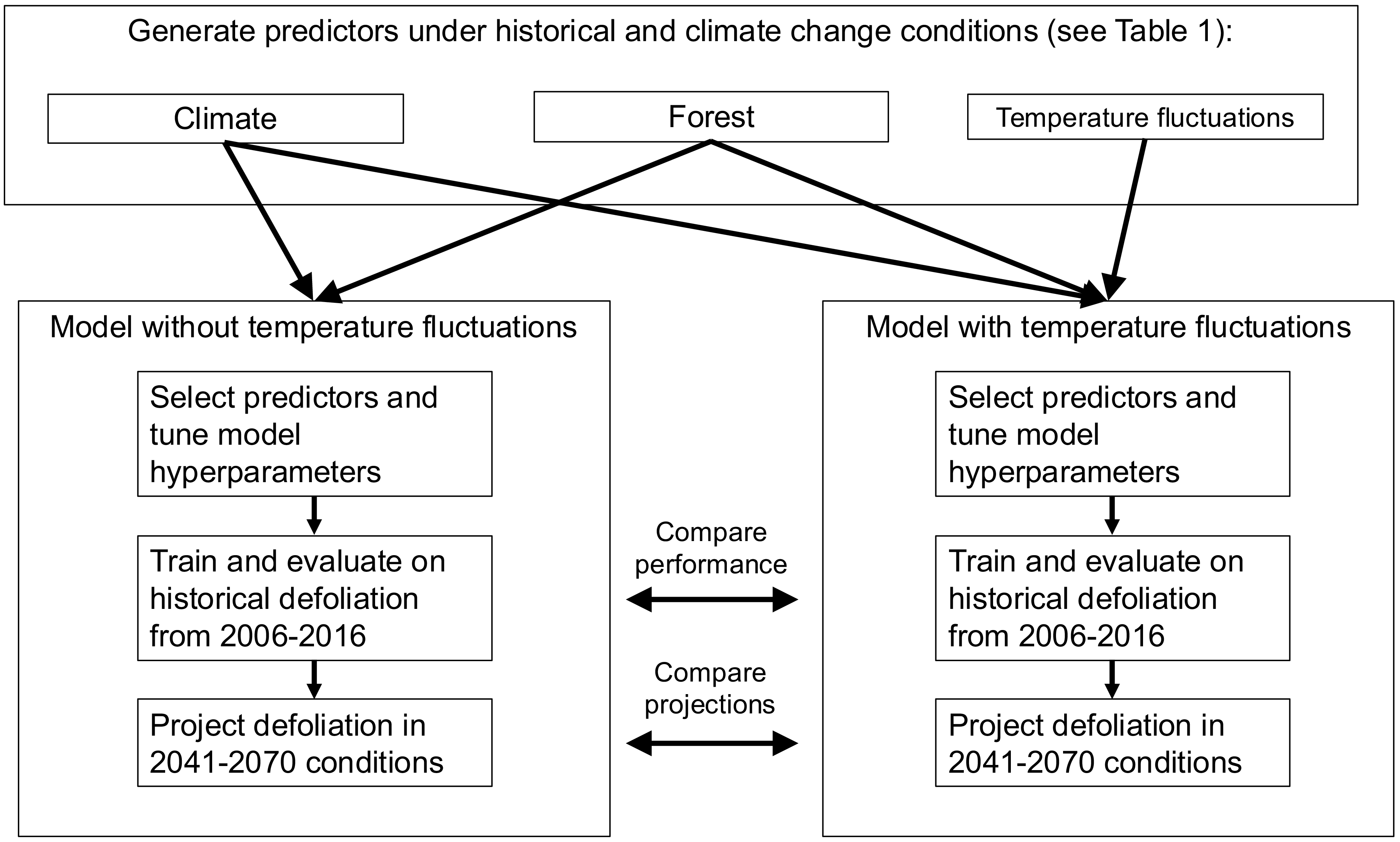
A general methods workflow is shown in Fig. 1. All analyses were performed using R, version 4.3.1 (R Core Team 2021).
General workflow of predictor generation and model tuning, training, evaluation, and prediction.

Figure 1. Long description
The flowchart begins with generating predictors under historical and climate change conditions, categorized into Climate, Forest, and Temperature fluctuations. These predictors are then used in two models: one without temperature fluctuations and one with temperature fluctuations. Each model involves selecting predictors and tuning model hyperparameters. Both models are trained and evaluated on historical defoliation data from 2006 to 2016. The models then project defoliation under future conditions from 2041 to 2070. The performance and projections of the two models are compared throughout the process.
Collecting and aggregating spruce budworm defoliation data
We used spruce budworm defoliation data collected by the Quebec Ministère des Ressources naturelles et des Forêts, which conducts annual aerial surveys of the province’s forests to record damage from major insect pests, the effects of disturbances such as forest fires, and the effectiveness of current pest control measures. During the surveys, spruce budworm defoliation patches are marked on a touchscreen computer from an aircraft travelling at 200 km/hour along flightlines spaced 4.5 km apart (Ministère des Ressources naturelles et des Forêts 2024). Survey locations are based on where insect damage was recorded the previous year, surveys of diapausing larvae, and predictive modelling of future outbreaks (Ministère des Ressources naturelles et des Forêts 2024). The location and severity of spruce budworm, Choristoneura fumiferana, defoliation patches are recorded during this survey (Ministère des Ressources naturelles et des Forêts 2024). Spruce budworm defoliation patches collected yearly from 1992 to 2006 (area = 2692.1 km2, npolygon = 4958), from 2007 to 2013 (area = 84 072.4 km2, npolygon = 54 867), and from 2014 to present (area = 774 851.7 km2, npolygon = 262 826 from 2014 to 2021) are stored as polygons in a publicly available file (see Supplementary material, Table S1 for links to data sources). The polygons have the following attributes: year of defoliation, defoliation severity level and score, hectares of defoliation, Quebec administrative region, and the geometric shape of the defoliation polygon. Yearly defoliation severity scores were mild (“1”) – with loss of foliage in the upper third of the crowns of some trees; moderate (“2”) – with loss of foliage in the upper half of the crowns of the majority of trees; and severe (“3”) – with loss of foliage along the entire length of the crowns of the majority of trees (Ministère des Ressources naturelles et des Forêts 2024). Tree mortality is not explicitly reported in aerial survey data. Cells that are reported as achieving high severity during the outbreak may be reclassified as moderate or mild later in the outbreak (Supplementary material, Fig. S1), indicating tree mortality is not counted as severe defoliation.
We also collected maps of spruce budworm defoliation in Ontario but did not use them in subsequent analyses due to difficulties standardising their data with the Quebec data (Supplementary material, File S1 – methods, and Fig. S2).
We projected defoliation polygons to a raster grid using the terra package (Hijmans et al. Reference Hijmans, Bivand, Forner, Ooms and Pebesma2021; Fig. 2) to model cumulative spruce budworm defoliation from the start of the most recent outbreak. Although year-over-year species distribution modelling approaches have been used to evaluate spruce budworm outbreaks (see Srivastava et al. Reference Srivastava, Tai, Robert and Carroll2024), we chose to evaluate the overall defoliation propensity of the environment by summarising defoliation intensity across all years studied. These summarised values also reduce the influence of biotic factors on outbreak dynamics explored by our model, which vary significantly across space and time over the course of an outbreak (Royama Reference Royama1984; Bouchard and Auger Reference Bouchard and Auger2014). We mapped the presence–absence of defoliation and the cumulative defoliation severity of each grid cell (i.e., how susceptible each cell was to spruce budworm damage) by summing the annual defoliation severity score of all polygons covering the centroid of a grid cell and assigning that value to the cell. Cumulative defoliation severity scores ranged from 0 (no defoliation) to a maximum of 21.84. Although yearly defoliation severity typically is reported as integers, bilinear interpolation of the cumulative defoliation grid to match the resolution of predictors led to noninteger cumulative severity values. The raster of spruce budworm defoliation in Quebec covered an area from –79.57° W to –61.55° W and from 45.42° N to 51.73° N. The grids had an initial resolution of approximately 412 m × 412 m; however, grids used in analyses were aggregated to a resolution of 300 arcsec (0.0833 × 0.0833 decimal degrees, or approximately 6.5 km × 6.5 km) to reflect distances between aerial survey flight lines (Ministère des Ressources naturelles et des Forêts 2024) and the resolution of climate predictors. All gridded variables use the EPSG:4326 (WGS84) coordinate reference system and are equal in latitude–longitude degree area but are not equal in squared kilometres (Office of Geomatics 2025).
Distribution of spruce budworm cumulative defoliation severity across Quebec from 2006 to 2016, collected from aerial surveys conducted by the Ministère des Ressources naturelles et des Forêts in Quebec. Cumulative defoliation severity is calculated by summing annual defoliation severity scores in each year from 2006 to 2016. Cells where defoliation is present have a mean cumulative defoliation severity of 6.63 ± 4.27 (standard deviation). An additional 35-km buffer with no measured defoliation was added to the mapped defoliation to serve as absences. n = 4146 grid cells (total area = 233 269 km2). Resolution: ∼6.5 km × 6.5 km.

Records of spruce budworm defoliation indicate that the current outbreak in eastern Canada began in 2006 (Natural Resources Canada 2021); we therefore used defoliation patches from that year onwards in our analysis. To confirm that defoliation polygons aligned with known outbreak years, we plotted the cumulative amount of defoliation in each grid cell in which defoliation was observed between 1997 and 2021. Cumulative defoliation severity increased rapidly in grid cells across Quebec from 2006 onwards (Supplementary material, Fig. S3). Although the outbreak beginning in 2006 is ongoing (Natural Resources Canada 2021), high-resolution daily climate records were only available until 2016. We therefore included only defoliation from 2006 to 2016 in our analyses.
Collecting and aggregating predictor data
We chose to evaluate the effect of four general predictor categories on defoliation presence and severity: forest, climate, degree-days, and temperature fluctuations. For a list of data sources, see Supplementary material, Table S1.
For forest predictors, we obtained raster grids of the forest composition of Canada, including the percent forest stand cover of spruce budworm host trees (white spruce, black spruce, balsam fir), and percent tree cover from the National Forest Inventory, a collaborative effort by federal, provincial, and territorial government agencies to generate continuous records of forest composition across Canada (Beaudoin et al. Reference Beaudoin, Bernier, Villemaire, Guindon and Guo2017). All grids had an initial resolution of 250 m × 250 m and were aggregated to approximately 6.5 km × 6.5 km using bilinear interpolation (Hijmans et al. Reference Hijmans, Bivand, Forner, Ooms and Pebesma2021).
For climate, temperature fluctuation, and degree-day predictors, we obtained minimum and maximum daily temperatures and daily precipitation from 2006 to 2016 across eastern Canada from the Climatologies at High Resolution for the Earth’s Land Surface Areas (CHELSA) dataset. The CHELSA dataset calculated global daily fine-resolution temperature and precipitation values up to 2016 using downscaling of atmospheric temperatures and climatologies (Karger et al. Reference Karger, Conrad, Böhner, Kawohl, Kreft and Soria-Auza2017, Reference Karger, Wilson, Mahony, Zimmermann and Jetz2021). Although many high-resolution climate products exist for our region of interest (e.g., Wang et al. Reference Wang, Hamann, Spittlehouse and Carroll2016), we selected CHELSA primarily because of its generation of global daily temperatures, which allowed us to generate daily temperature fluctuation counts across a broad geographic region, and its generation of global monthly climate variables under several climate change scenarios. In addition, CHELSA’s global distribution allows our methods to be more easily extrapolated to other species and regions of interest around the world.
From the daily CHELSA temperature values, we calculated the annual mean temperature, annual mean minimum temperature, annual maximum temperature, the absolute annual minimum temperature, and the absolute annual maximum temperature. We calculated these values for each month of the year, averaged across 2006–2016. We also obtained daily precipitation values from CHELSA to calculate mean yearly and monthly precipitation. For the degree-day predictors, using the CHELSA data, we summed the difference between mean daily temperatures and 0 °C annually and in each month, averaged across 2006–2016. Maps of historical climate and degree-day data covered an area from –83.57° W to –57.55° W and from 41.42° N to 55.73° N, with a resolution of approximately 6.5 km × 6.5 km.
To obtain temperature fluctuation predictors across the landscape, we calculated repeated temperature exposures, or the number of times the temperature in each grid cell crossed a particular daily temperature threshold each month (e.g., the number of times the temperature crossed 0 °C daily in January). Temperature thresholds were chosen based on temperature treatments performed by Marshall and Sinclair (Reference Marshall and Sinclair2015) on second-instar spruce budworm, temperature thresholds regularly experienced within the spruce budworm range in Quebec, and predominant periods of temperature fluctuations identified by Dillon et al. (Reference Dillon, Woods, Wang, Fey, Vasseur and Telemeco2016). To calculate temperature fluctuation predictors, we interpolated the daily minimum and maximum temperatures from CHELSA to simulate change in daily temperature across an entire year at each grid cell. We then summed the number of times the temperature in each cell crossed from below to above a particular threshold (e.g., 0–10 °C) to calculate the frequency of temperature exposure (Supplementary material, Fig. S4). We averaged these values across 2006–2016 and transformed the points into a raster map with a resolution of approximately 6.5 km × 6.5 km. To validate temperature fluctuation predictors, we compared CHELSA daily temperatures to hourly weather station records at two locations within the defoliated region (Supplementary material, Table S2, Fig. S5). We found that at both locations, the frequency of temperature threshold crossings calculated by our method varied slightly from hourly weather station records. However, the slopes of the relationships between the threshold crossings calculated from these two weather data sources did not differ significantly from 1 at both locations. Overall, we generated a total of 169 climate, forest, and temperature fluctuation predictors (Table 1).
List of predictors used for species distribution modelling with description of predictors, number of predictors generated in each category, predictors selected for final models by pruning using correlation coefficients and variance inflation factors, and the rationale for initial inclusion in the model. TF, retained in temperature fluctuation model; NTF, retained in no temperature fluctuations model; Both, selected for both models; Neither, selected for neither model.

Table 1. Long description
A table with 35 rows and 5 columns. The columns are labeled Predictor, Description, Number of predictors, Selected for final model (TF/NTF/Neither), and Rationale. The table lists various forest, climate, and temperature fluctuation predictors used for modeling. Each row provides details on the predictor’s description, the number of predictors in each category, which model they were selected for, and the rationale for their inclusion. The predictors are grouped into forest predictors, climate predictors, temperature fluctuation predictors, and degree-day predictors. Each group has specific columns filled with relevant data.
To determine the influence of temperature fluctuations on predicted future defoliation, we regenerated model predictors under simulated climate change conditions from 2041 to 2070. Because tree species in the eastern Canadian boreal forest show limited migration ability under climate change conditions (Boisvert-Marsh et al. Reference Boisvert-Marsh, Pedlar, de Blois, Le Squin, Lawrence and McKenney2022) and the majority of reductions in forest area under shared socioeconomic pathway (SSP) climate scenarios are expected to occur outside of North America (Böttinger and Kasang, Reference Böttinger and Kasangno date; Popp et al. Reference Popp, Calvin, Fujimori, Havlik, Humpenöder and Stehfest2017), we used the same tree distributions that are used in the historical models (Beaudoin et al. Reference Beaudoin, Bernier, Villemaire, Guindon and Guo 2017).
To generate climate, degree-day, and temperature fluctuation variables under climate change conditions, we used the monthly CHELSA Coupled Model Intercomparison Project, phase 5–(CMIP5–) predicted climatologies for 2041–2070 (Karger et al. Reference Karger, Conrad, Böhner, Kawohl, Kreft and Soria-Auza2017). These represent monthly temperatures in an example year under different climate change scenarios and were generated using the Geographic Fluid Dynamics Laboratory Earth System Model, version 4 (GFDL-ESM4; Alvich, Reference Alvichno date). We selected climatologies from the SSP370 climate scenario, which predicts a moderate-to-high amount of future global emissions (Böttinger and Kasang, Reference Böttinger and Kasangno date). Although the SSP370 climate scenario includes substantial land-use and aerosol emission changes in addition to increased greenhouse gas emissions, these have a limited effect on projected solar radiation and precipitation in eastern Canada compared to emissions changes in other SSP scenarios (Shiogama et al. Reference Shiogama, Fujimori, Hasegawa, Hayashi, Hirabayashi and Ogura2023). Furthermore, the majority of land-use changes in the SSP370 scenario are projected to occur outside of North America (Popp et al. Reference Popp, Calvin, Fujimori, Havlik, Humpenöder and Stehfest2017). To simulate daily temperatures under this climate change scenario, we used the R multi-sites auto-regressive weather generator (RMAWGEN) synthetic weather generator package (Nandan et al. Reference Nandan, Bandaru, Meduri, Jones and Lollato2024; Cordano et al. Reference Cordano, Eccel and Luedeling2025) implemented through the chillR package (Luedeling et al. Reference Luedeling, Caspersen and Fernandez2023) to generate daily stochasticity from the monthly CHELSA climate change projections. This package uses the CHELSA monthly projections to guide future climatic trends in the stochastic data and historical daily temperatures from the 2010–2016 CHELSA data to interpolate stochastic daily minimum and maximum temperatures (Supplementary material, Fig. S6). From the daily stochastic weather output, we generated annual and monthly climatic predictors, degree-day predictors, and temperature fluctuation predictors under SSP370 climate change conditions. Because we were predicting into the future and the range of the eastern spruce budworm is expected to shift (Gray Reference Gray2008; Régnière et al. Reference Régnière, St-Amant and Duval2012b), we increased the spatial extent of the predictors to include –96.76° W to –59.51° W and 43.42° N to 53.76° N. All predictors had a spatial resolution of approximately 6.5 km × 6.5 km.
Building and evaluating distribution models of defoliation
Although spruce budworm is found endemically throughout much of Canada’s boreal forest (Marshall and Roe Reference Marshall and Roe2021), only certain populations transition to epidemic (or outbreaking) dynamics with densities high enough to cause detectable defoliation. Therefore, “absences” in our model are defined as areas where no defoliation was observed and where populations remain at low endemic densities rather than as areas where spruce budworms are completely absent. We marked cells up to 35 km away from the nearest point with defoliation as regions where defoliation was not detected, creating a buffer region around the outbreak. This buffer distance is within the local and long-distance dispersal capability of spruce budworm (Greenbank et al. Reference Greenbank, Schaefer and Rainey1980; Sturtevant et al. Reference Sturtevant, Achtemeier, Charney, Anderson, Cooke and Townsend2013) but where no defoliation was recorded by aerial surveys. A larger buffer area would exceed the extent and precision of aerial surveys, which can be affected by flight conditions and human error (Ministère des Ressources naturelles et des Forêts Reference Nandan, Bandaru, Meduri, Jones and Lollato2024) and would offer limited additional information for distinguishing conditions associated with defoliation (Barve et al. Reference Barve, Barve, Jiménez-Valverde, Lira-Noriega, Maher and Peterson2011). Tree cover did not differ significantly between the buffer regions and areas where defoliation was present, so no additional filtering of buffer cells was performed. We also ensured grid cells used for training the models were within Quebec provincial boundaries.
Exploratory modelling showed that random forest regression had the highest r 2-value (best preliminary performance) amongst several machine learning algorithms tested; therefore, it was selected for further modelling analysis. To generate honest and spatially unbiased metrics of model performance, we used spatial cross-validation to reduce the effect of spatial autocorrelation on model evaluation. To do this, we used the spatialRF package (Wright and Ziegler Reference Wright and Ziegler2017), which generates random forest models, evaluates the contributions of predictors locally and to overall model performance, and evaluates model performance and transferability using spatial cross-validation. We chose to evaluate the influence of temperature fluctuation predictors on defoliation using a random forest regression model predicting cumulative defoliation severity (i.e., summed severity scores).
Climate, degree-day, forest, and temperature fluctuation predictors were highly correlated with one another, and a model with all predictors showed a high degree of overfitting and poor overall performance. Due to the potentially complex and nonparametric relationships between predictors and defoliation, we ran an initial model with all 169 predictors and default spatialRF hyperparameters (values configuring the random forest algorithm; Wright and Ziegler Reference Wright and Ziegler2017) and obtained the ranked relative importance of each predictor measured by permutation. We then kept predictors with a high relative importance in the initial model and eliminated less-important predictors with a correlation coefficient above 0.95 and subsequently a variance inflation factor higher than 7.5 as compared to higher-ranking predictors (i.e., if two predictors are highly correlated with one another, the predictor with a higher importance to the initial model is kept and the other is removed; Zhang et al. Reference Zhang, Leroux, Bowden, Hargan, Hurford and Moise2023). These values are more conservative than those used in similar models (Dormann et al. Reference Dormann, Elith, Bacher, Buchmann, Carl and Carré2013); however, due to the large number of variables that were highly correlated with one another, we decided more restrictive predictor selection was needed. This significantly reduced the number of predictors in the final model with all predictor categories from 169 to 12 predictors and in the model trained without fluctuations from 96 to 8 predictors. Degree-day predictors were not selected by this process; therefore, they were absent from subsequent analysis.
As some host tree predictors were not selected during predictor pruning, they were added back in to ensure predictions of defoliation under climate change were limited by the distribution of suitable food and habitat (which are not expected to change significantly under climate change scenarios; Boisvert-Marsh et al. Reference Boisvert-Marsh, Pedlar, de Blois, Le Squin, Lawrence and McKenney2022). We then retuned model hyperparameters using the spatialRF function “rf_tuning.” Inclusion of deselected forest variables increased the variance inflation factor and correlation coefficients amongst predictors in the final model. However, measures of model performance that were trained on only initially selected predictors and no deselected forest variables did not significantly differ or were slightly worse than those of the model that included deselected forest variables (mean absolute error = 0.62, 95% confidence interval = 0.60–0.65; root mean square error = 2.66; 95% confidence interval = 2.65–2.67), indicating their inclusion has little effect on performance.
To evaluate the model and to determine the importance of selected predictors, we calculated the mean absolute error of predictions of historical cumulative defoliation severity and the average increase in error when individual predictors were scrambled by permutation (Wright et al. Reference Wright, Ziegler and König2016). These metrics are based on predictions made on out-of-bag data (grid cells not used to train the random forest model). We also performed cross-validation that was repeated across 100 spatial folds with a 4:1 training:testing data split to measure the root mean square error of the regression model (Wright and Ziegler Reference Wright and Ziegler2017). For evaluation and climate change projections, the model predicted the cumulative defoliation severity score. To determine the effect of temperature fluctuation predictors on model performance, we built and evaluated a second model that did not include temperature fluctuation predictors. Predictor pruning using the correlation coefficient and variance inflation factor was performed on climate and forest predictors only, using the same protocol as the initial model, and model hyperparameters were retuned for this model to ensure the differences in performance were not due to poorly adapted model hyperparameters (Wright and Ziegler Reference Wright and Ziegler2017). To determine whether performance (the root mean squared error) of the models with and without temperature fluctuations differed significantly across the 100 spatial cross-validation folds, we performed a Mann–Whitney–Wilcoxon test.
To determine where the model performed more poorly, we investigated whether model error (residuals) varied systematically across the region. We also generated partial dependence plots to visualise the relationships between predictors and defoliation severity. Partial dependence plots show the relationship between the value of a predictor and the value of the predicted defoliation propensity generated by the model across fixed quantiles of other predictors (0.2 = predictors fixed at the 20th percentile, 0.5 = predictors fixed at the median value, 0.8 = predictors fixed at the 80th percentile; Benito Reference Benito2021). This can be used to infer the effect of the predictor on spruce budworm defoliation from the complex relationships amongst predictors and defoliation.
Predicting defoliation under 2040–2071 climate change conditions
We used the random forest regression to predict regions across Quebec, Ontario, and Labrador, Canada (from –96.76° W to –59.51° W and from 43.42° N to 53.76° N) that may be at risk of defoliation in a simulated 2040–2071 climate scenario. These simulated years occur 15–45 years after the collapse of the current outbreak and should capture the next bout of defoliation, based on historical outbreak patterns (Boulanger and Arseneault Reference Boulanger and Arseneault2004). We provided the model with the CHELSA CMIP5 climatology predictors and existing host tree distributions and had the model predict cumulative defoliation across the region. Then, to determine the effect of temperature fluctuations on predictions of defoliation under climate change, we repredicted cumulative defoliation under climate change conditions using the model trained without temperature fluctuation predictors. To measure the effect of temperature fluctuations, we reported deviations in cell-by-cell predictions between the full model and the model with temperature fluctuation predictors removed and investigated differences in the distribution of predicted defoliation. We calculated area under the curve (AUC) for each model to quantify the total number of grid cells that have predicted cumulative defoliation severity values greater than 4 and compared the tendency of models with and without temperature fluctuations to predict more severe defoliation. We also reported the number of grid cells with cumulative severity values greater than 4 across the latitudinal range of predicted defoliation to determine if including temperature fluctuations influences the distribution of more severe defoliation across the landscape.
Results
Overall model performance
Overall, the full regression model predicted historical cumulative defoliation severity with a mean absolute error of 0.54 (95% confidence interval = 0.52–0.56) across 4146 cells with a range of actual severity scores from 0 to 21.84 and a mean root mean square error of 2.73 (95% confidence interval = 2.67–2.79) across 100 spatial folds during evaluation. Although both mean absolute error and root mean square error report model error, root mean square error is based on spatial cross-validation rather than on out-of-bag predictions. The model trained without temperature fluctuation variables had a mean absolute error of 0.60 (95% confidence interval = 0.58–0.62) and a mean root mean square error of 3.00 (95% confidence interval = 2.91–3.09). Model error across spatial folds significantly increased in the model trained without temperature fluctuation predictors when root mean square errors were compared (W = 3127, P < 0.01, Mann–Whitney–Wilcoxon test).
To understand where the regression model performed more poorly, we investigated the residuals of the regression model along a gradient of defoliation severity. We tested both a polynomial fit and a linear fit and found that model error increased along a gradient of defoliation severity when grid cells where defoliation was present were considered (linear regression fit: R 2 = 0.37, F1,1479 = 866.3, P < 0.001; Fig. 3). Although the relationship between residuals and defoliation severity was fitted similarly by a polynomial (corrected Akaike information criterion (AICc) = 2863.22) and linear regression (AICc = 2863.76; ΔAICc = 0.55), we selected the simpler linear model. Grid cells where no defoliation was observed showed a wide range of residuals, but generally defoliation absence was predicted accurately (Fig. 3B, y-axis histogram).
Regression model error tends to increase in areas with higher observed defoliation severity: A, distribution of residuals of random forest regression model. Red cells indicate model underestimated defoliation severity, blue cells indicate model overestimated defoliation severity; B, relationship between model residuals and actual values of cumulative defoliation severity. Histograms in margins show the density of data across x-axis and y-axis values. Linear regression line only fits to cumulative defoliation severity (x-axis) values higher than zero (where defoliation was present). n present = 1481 grid cells.

Figure 3. Long description
Panel A: A map shows the distribution of residuals of a random forest regression model. Red cells indicate areas where the model underestimated defoliation severity, while blue cells indicate areas where the model overestimated defoliation severity. The map covers a region with latitude ranging from 45 degrees North to 52 degrees North and longitude ranging from 60 degrees West to 80 degrees West. Panel B: A scatter plot illustrates the relationship between model residuals and actual values of cumulative defoliation severity. The x-axis represents cumulative defoliation severity, and the y-axis represents residuals. Histograms in the margins show the density of data across x-axis and y-axis values. A linear regression line fits to cumulative defoliation severity values higher than zero, indicating the relationship between defoliation severity and model error. The scatter plot includes 1481 grid cells.
Predictor contributions
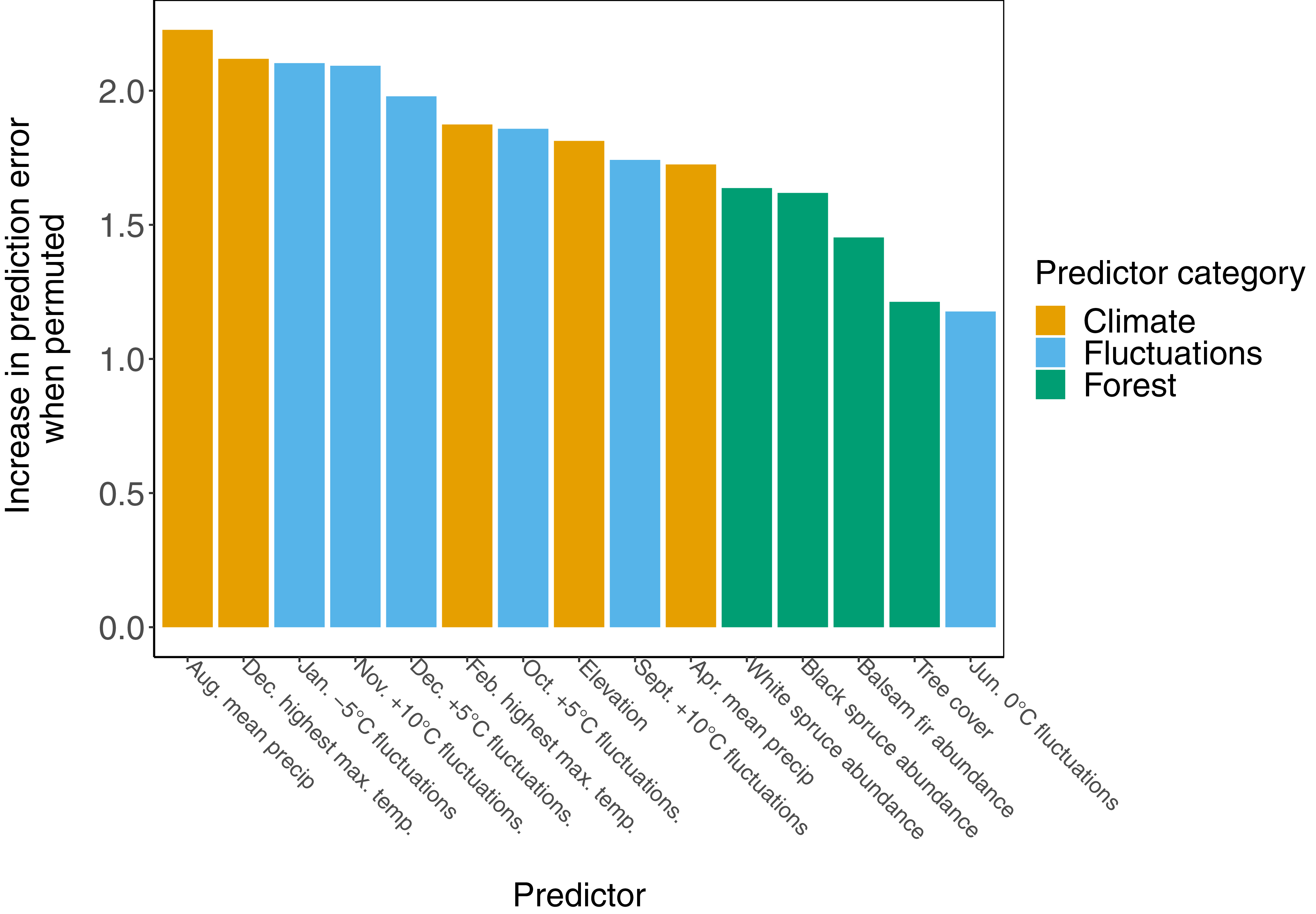
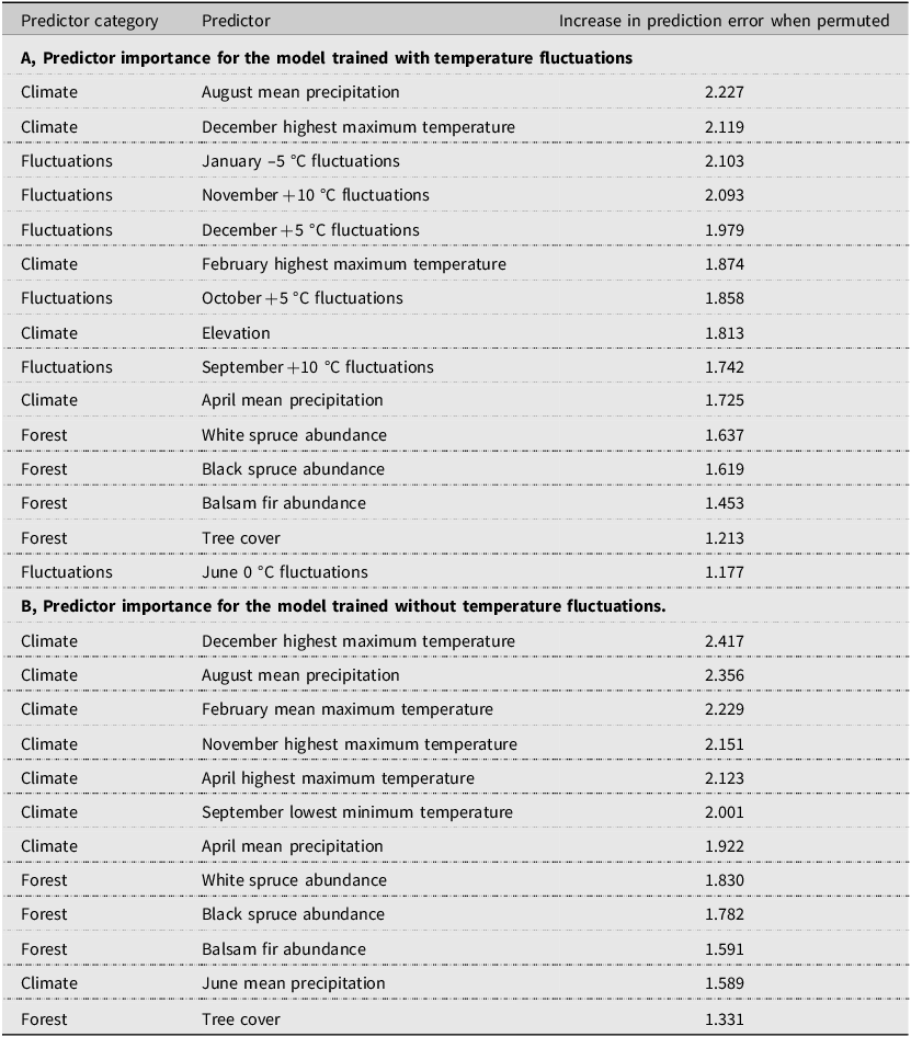
Climate and temperature fluctuation predictors had the highest overall importance in the random forest regression model, with a mean increase in out-of-bag prediction error when permuted of 1.95 ± 0.21 (standard deviation) and 1.83 ± 0.35 (standard deviation), respectively (Fig. 4; Table 2A, B). Forest composition predictors had lower overall importance, with a mean increase in error when permuted of 1.48 ± 0.20 (standard deviation). The distribution of local (cell-by-cell) importance of the top four most important variables also varies among predictors, with some showing higher importance that is localised to areas where defoliation is present or absent. For example, August mean precipitation generally had higher importance in areas where defoliation was present, whereas January –5 °C fluctuations were generally more important in areas where defoliation was absent (Supplementary material, Fig. S7). Temperature fluctuation predictors make up six of 15 predictors in the model and rank relatively highly among other predictors. Five of six temperature fluctuation predictors rank more highly than all tree distribution predictors.
Climate and temperature fluctuation predictors are generally more important than forest predictors in the random forest regression model. Bars represent an increase in prediction error on out-of-bag data when the predictor was scrambled by permutation.

Ranked predictor importance for defoliation models: A, model trained with temperature fluctuation predictors; and B, model trained without temperature fluctuation predictors. Importance represents the mean increase in prediction error on out-of-bag data after scrambling predictor by permutation. See Table 1 for detailed predictor descriptions.

Table 2. Long description
A table with two sections, A and B, each showing predictor importance for models trained with and without temperature fluctuations. Section A has 15 rows and 3 columns, listing predictors categorized under Climate, Fluctuations, and Forest, along with their increase in prediction error when permuted. Section B also has 12 rows and 3 columns, similarly listing predictors and their increase in prediction error. Each section includes specific predictors and their respective error increases, with Section A focusing on model with temperature fluctuations and Section B on models without.
The relationships between cumulative defoliation severity and model predictors in the regression model are complex and depend on the fixed quantiles of other predictors (Fig. 5). Generally, defoliation is more severe with lower August mean precipitation and higher April mean precipitation. Defoliation severity also increases at lower elevations and with higher tree cover, although relationships with specific tree species are variable. Generally, no consistent relationship was found between defoliation severity and fluctuation predictors because these vary across months, temperatures, and quantiles of other predictors. (Supplementary material, Fig. S8 shows the relationships between values of the four most important predictors and observed and predicted defoliation.)
Relationship between random forest regression model predictors and predicted cumulative defoliation severity. Lines show how each predictor individually affects model predictions across fixed quantile values of other predictors. Quantiles of 0.2, 0.5, and 0.8 correspond to predictors fixed at the 20th percentile, predictors fixed at the median value, and predictors fixed at the 80th percentile, respectively. Precipitation predictors transformed from kg m–2 s–1 to mg m–2 s–1 for ease of plotting and interpretation. Additional information on predictors can be found in Table 1.

Climate change predictions
In general, the regression models trained with and without temperature fluctuation were able to identify areas with environmental conditions correlated with defoliation when predicting with CMIP5 predicted climatologies for 2041–2070 (Fig. 6A, B). The model trained with temperature fluctuation variables had a mean predicted cumulative defoliation severity of 2.44 ± 0.68 (standard deviation) and predicted the greatest cumulative defoliation severity as 4.87. The range of predicted cumulative defoliation severity is highly reduced from the training data (maximum severity of 21.84). The model trained without temperature fluctuation variables predicted greater cumulative defoliation, on average, with a mean predicted cumulative defoliation severity of 3.03 ± 0.64 (standard deviation). This model also predicted a higher maximum cumulative defoliation severity, with a maximum predicted value of 6.70. However, this is still significantly reduced from the training data.
Predicted future defoliation across Quebec, Ontario, and Labrador by the random forest regression model using CMIP5-predicted climatologies for 2041–2070. Areas covered by lakes and rivers removed from the prediction area: A, distribution of predicted cumulative defoliation severity of the model trained using temperature fluctuations; B, distribution of predicted cumulative defoliation severity of the model trained without temperature fluctuations; C, difference in predicted defoliation severity between models trained with and without temperature fluctuations; D, the model trained using temperature fluctuations (left panel) predicted severe (> 4 cumulative severity score) defoliation less and with a more northerly distribution than the model trained without using temperature fluctuations (right panel).

Figure 6. Long description
Panel A: A heat map showing the distribution of predicted cumulative defoliation severity using a model trained with temperature fluctuations. The color gradient ranges from green (low severity) to red (high severity). Panel B: A heat map displaying the distribution of predicted cumulative defoliation severity using a model trained without temperature fluctuations, with a similar color gradient. Panel C: A difference map illustrating the predicted defoliation severity between models trained with and without temperature fluctuations, using a colour gradient from blue (model without fluctuations predicted higher defoliation) to beige (no difference) to red (model with fluctuations predicted higher defoliation). Panel D: Two line graphs showing the frequency of cells with severity greater than 4, comparing the model trained with temperature fluctuations (left) and without temperature fluctuations (right). The y-axis represents latitude, and the x-axis represents the frequency of cells.
The regression model trained with temperature fluctuations predicted severe defoliation at a lower frequency than did the model trained without temperature fluctuations, but in more northerly regions (Fig. 6). The frequency of cells with a predicted cumulative defoliation severity greater than 4 was found to be much higher in the model trained without temperature fluctuations (AUCwith fluctuations = 101 versus AUCwithout fluctuations = 2421, respectively). The average latitude of cells with a defoliation severity greater than 4 was 51.1 ± 1.54 (standard deviation) in the model trained with temperature fluctuations and 49.4 ± 1.66 (standard deviation) in the model without. However, given that higher defoliation severity is forecast to occur near to the highest latitudes included in the model runs, the latitudinal extent of the study area may be artificially truncating defoliation predictions.
Discussion
In the present study, we show the utility of including physiologically informed predictors in species distribution models, finding temperature fluctuations are highly correlated with cumulative spruce budworm defoliation from 2006 to 2016 in Quebec. Including temperature fluctuations improved the performance of the random forest regression model of defoliation propensity and influenced predictions of future defoliation under climate change. Temperature fluctuation predictors ranked highly amongst model predictors and had a similar mean importance to climate predictors and greater importance than forest predictors did. When predicting future defoliation under climate change conditions, including temperature fluctuation predictors drastically reduced predicted defoliation severity across the landscape. These results suggest that temperature fluctuations play a role in influencing landscape-scale defoliation by spruce budworm and demonstrate the utility of incorporating physiological measures into species distribution models of ectotherms to improve performance.
The importance of temperature fluctuations to the defoliation regression model was expected given the physiological importance of temperature fluctuations to spruce budworm in the laboratory and to other ectotherms generally. Marshall and Sinclair (Reference Marshall and Sinclair2015) demonstrated that the number and frequency of low-temperature stress events experienced affected spruce budworm survival in the laboratory, which supports our findings that temperature fluctuations may be important on a landscape scale. Those authors’ results also indicate that the frequency of temperature fluctuations may be more important than duration and severity of temperature exposure, which was not the case in our model, given the importance of other climatic variables. In addition, our model suggests that fluctuations at mild temperatures during the fall and winter may influence defoliation severity over the landscape. How the frequency of mild-temperature exposures may affect spruce budworm and other ectotherms during the fall and winter has not been directly studied; however, short exposures to warm-temperature events are known to affect the fitness of spruce budworm and other insects, particularly when they occur before or during overwintering in the fall and winter. Roe et al. (Reference Roe, Wardlaw, Butterson and Marshall2024) found that diapause preparation in spruce budworm is highly sensitive to fall length and temperature and that there is a delicate balance between survival and energetic costs during this period. Prolonged exposure to higher temperatures before overwintering also led to significant delayed post-overwintering mortality in the green-veined white, Pieris napi (Lepidoptera: Pieridae) (Nielsen et al. Reference Nielsen, Lehmann and Gotthard2022). Therefore, although there is no direct correlation between spruce budworm fitness and mild temperature fluctuations in fall and winter, it is plausible that such a relationship may exist, and we suggest further study to identify mechanistic explanations.
In general, the importance in the present study of climate predictors to the random forest regression model was consistent with findings from previous spruce budworm species distribution models (Candau and Fleming Reference Candau and Fleming2005; Gray Reference Gray2008; Zhang et al. Reference Zhang, Leroux, Bowden, Hargan, Hurford and Moise2023) and environmental factors known to affect spruce budworm physiology and defoliation. Winter (December and February) maximum temperatures and spring and summer (April and August) precipitation were the most important climate predictors to our model. The importance of winter maximum temperatures is consistent with the spruce budworm distribution model created by Candau and Fleming (Reference Candau and Fleming2005), who identified this factor as the most important variable for predicting defoliation frequency during a 1967–1998 outbreak in Ontario. Given the effect of winter temperatures on insect cold stress and overwintering survival and fitness (Sinclair Reference Sinclair2015; Marshall and Roe Reference Marshall and Roe2021), it is logical that winter temperatures may also drive spruce budworm fitness at the landscape scale.
Precipitation was also important for predicting defoliation in the present study; in particular, August precipitation was the most important individual predictor of defoliation in our regression model. Studies on spruce budworm show that periods of drought can promote defoliation (Wellington et al. Reference Wellington, Fettes, Belyea and Turner1950) and that larval development is faster in summers with dry and sunny weather (Greenbank Reference Greenbank1956); however, spruce budworm moths have generally eclosed by August, so climatic conditions in this month likely do not have a direct effect on larval defoliation (Marshall and Roe Reference Marshall and Roe2021). Peak spruce budworm moth exodus typically occurs in July and August (Royama Reference Royama1984): lower tropospheric weather conditions in this month influence dispersal (Boulanger et al. Reference Boulanger, Fabry, Kilambi, Pureswaran, Sturtevant and Saint-Amant2017) and may partially explain our results. Our results match the spruce budworm defoliation model created by Zhang et al. (Reference Zhang, Leroux, Bowden, Hargan, Hurford and Moise2023), who also found that spring and summer precipitation levels are strong predictors of defoliation during an outbreak in Newfoundland, Canada. Ultimately, our results align with previous findings on the climatic drivers of defoliation and underscore the influence of climate and weather on spruce budworm outbreak dynamics.
Our model provides insights into the factors influencing the distribution and severity of spruce budworm defoliation; although these insights are ultimately correlative, they are supported by physiological mechanisms and provide a case study for incorporating physiology into species distribution models. Correlative models use climate and environmental factors to predict the response of an organism to changes in those factors and have been used effectively to investigate the drivers of landscape-scale spruce budworm outbreaks (Candau and Fleming Reference Candau and Fleming2005; Gray Reference Gray2008; Zhang et al. Reference Zhang, Leroux, Bowden, Hargan, Hurford and Moise2023). However, these models do not consider organism physiology or sub-processes, which can modify the organism’s response to different conditions and inform their responses to climate change (Maino et al. Reference Maino, Kong, Hoffmann, Barton and Kearney2016). Therefore, robust predictions of ectotherm distributions in changing conditions require an understanding of the physiological mechanisms driving the ectotherms’ response in addition to landscape-level studies of abundance and fitness using modelling techniques (Rodríguez et al. Reference Rodríguez, García, Carreño and Martínez2019). Our model demonstrates that incorporating spatial predictors that directly relate to species survival and fitness is possible, improves species distribution model performance, and adds to a growing body of work on “hybrid” species distribution modelling that combine mechanistic and correlative approaches (Tourinho and Vale Reference Tourinho and Vale2023). These model principles may also be extended by incorporating explicitly mechanistic methods, such as biophysical modelling (Lembrechts et al. Reference Lembrechts, Nijs and Lenoir2019; Kearney and Porter Reference Kearney and Porter2020), into correlative species distribution models.
Although our model attempts to capture how environmental factors influence spruce budworm defoliation, biotic factors may still explain the greater model error in areas of severe defoliation. The dynamics of spruce budworm outbreaks are complex and likely are driven by a combination of top-down and bottom-up factors (Pureswaran et al. Reference Pureswaran, Johns, Heard and Quiring2016). Therefore, greater model error in areas with high defoliation severity may be explained by spruce budworm population dynamics and defoliator–host tree relationships. De Grandpré et al. (Reference De Grandpré, Marchand, Kneeshaw, Paré, Boucher and Bourassa2022) found that spruce budworm herbivory significantly increases tree needle nitrogen content, which may lead to a positive feedback loop of improved host foliage quality that promotes further spruce budworm feeding and development. In addition, dispersal of gravid moths can synchronise outbreaks across the landscape (Régnière and Nealis Reference Régnière and Nealis2019), and spruce budworm population spread, growth rates, and outbreak risk are known to be density-dependent (Régnière et al. Reference Régnière, Cooke, Béchard, Dupont and Therrien2019). Finally, climate change is expected to have significant and complex effects on spruce budworm physiology and outbreak dynamics (Navarro et al. Reference Navarro, Morin, Bergeron and Girona2018; Boulanger et al. Reference Boulanger, Desaint, Martel, Marchand, Tonye, Saint-Amant and Régnière2025), including outbreak frequency (Candau and Fleming Reference Candau and Fleming2011), length, and intensity (Gray Reference Gray2008). Therefore, although models investigating environmental factors such as defoliation are useful, additional drivers contributing to outbreak dynamics that are not as easily modelled, such as biotic interactions and the complex effects of climate change, should be considered in future work.
Shifts in the frequency of temperature fluctuations under climate change may influence the future distribution of spruce budworm and other ectotherms, but challenges still exist when modelling future daily temperatures and how biota will respond to climate change. Although the accuracy of future model predictions cannot be evaluated, the predicted propensity to defoliation under climate change by the model that we trained with temperature fluctuations was dramatically different than that predicted by the model trained without temperature fluctuations, suggesting that models are highly sensitive to these predictors. Overall temperature variability is expected to increase under climate change (Wang and Dillon Reference Wang and Dillon2014; Dillon et al. Reference Dillon, Woods, Wang, Fey, Vasseur and Telemeco2016); however, the frequency of variation at specific temperature thresholds is strongly driven by warming fall, winter, and spring temperatures and the nonuniformity of climate change effects across biomes and latitudes (Marshall et al. Reference Marshall, Gotthard and Williams2020; Contosta et al. Reference Contosta, Arndt, Baulch, Casson, Harpold and Morelli2024). This was reflected in our results, with changes in the frequency of temperature fluctuation predictors under climate change varying widely across the landscape and among our predictors as we saw a general decrease in the frequency of mild fall temperatures and a general increase in the frequency of mild winter temperatures (unpublished data). This also highlights uncertainty in species distribution model predictions: although our methods could generate stochastic daily temperatures informed by both daily historical temperatures and future climate trends, there is no reliable way to validate these future daily temperatures, and our methods may not accurately forecast trends in temperature fluctuations – and, by extension, spruce budworm defoliation and species distributions – in the future. Furthermore, the trajectory of climate change and its global and regional effects remain uncertain (Böttinger and Kasang, Reference Böttinger and Kasangno date). More reliable methods to predict future daily maximum and minimum temperatures are being developed (Dillon et al. Reference Dillon, Woods, Wang, Fey, Vasseur and Telemeco2016; Araya-Osses et al. Reference Araya-Osses, Casanueva, Román-Figueroa, Uribe and Paneque2020; Requena et al. Reference Requena, Nguyen, Burn, Coulibaly and Nguyen2021), but few resources on a fine spatial and temporal scale useful for large-scale biogeographical forecasting exist at the present time. The sensitivity of our species distribution model to temperature fluctuations and the lack of fine-scale future daily weather forecasting reveal uncertainty when predicting the response of biota to climate shifts. To combat this, we suggest further refinement of our methods and development of more fine-scale future climate modelling to clarify the response of spruce budworm and other ectotherms to daily temperature fluctuations under climate change.
Conclusion
In the present study, we investigated the hypothesis that including physiologically informed predictors in a species distribution model improves forecasts of the landscape-scale distribution of spruce budworm defoliation. Results from our defoliation model suggest temperature fluctuations are correlated with historic spruce budworm defoliation in Quebec and are as important to the model as climatic variables are. Furthermore, including temperature fluctuation variables drastically decreased predicted defoliation severity across Ontario, Quebec, and Labrador under climate change conditions. Further study is needed to clarify the role of biotic drivers of outbreaks on defoliation patterns and to generate reliable and large-scale future daily temperatures to more accurately evaluate the response of insects to future climate shifts. Ultimately, elucidating the effects of temperature fluctuations and other climatic factors on spruce budworm defoliation reveals a link between physiological responses and landscape-scale fitness that should be considered when building species distribution models of ectotherms. Given the highly destructive nature of spruce budworm, the model we developed will help to improve understanding of the drivers of forest pest outbreaks to enable better prediction of regions susceptible to large-scale outbreaks. The effects of temperature fluctuations on survival and fitness are common across ectotherm taxa, and our model provides a novel and useful framework for incorporating daily temperature variation into species distribution modelling of ectotherms.
Supplementary material
The supplementary material for this article can be found at https://doi.org/10.4039/tce.2026.10069.
Data availability statement
All data used in the study are publicly available and can be found in Supplementary material, Table S1. Code used in analyses, full-sized figures, supplementary material, and Supplementary material, Table S1 containing links to data are available at https://osf.io/anxc2/overview?view_only = 1332727e7f244169b6a4bb8d2eb8a0ce.
Acknowledgements
The authors thank Dr. Amanda Roe, Ian DeMerchant, and Adam Hogg for their assistance in accessing and providing spruce budworm defoliation data, as well as the Ministère des Ressources naturelles et des Forêts and the National Forest Inventory for data collection and curation. The authors additionally thank Dr. Amanda Roe, for her invaluable knowledge on spruce budworm and project guidance, and Dr. Allan Carroll, for his guidance on modelling forest insect pests. They thank Dr. Amy Angert and Dr. Bill Milsom for their comments, which significantly improved the preliminary manuscript, and the anonymous peer reviewers for their valuable input, which significantly improved the manuscript.
Competing interests
The authors have no competing interests to report.




 Open access

