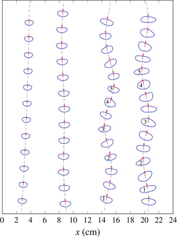
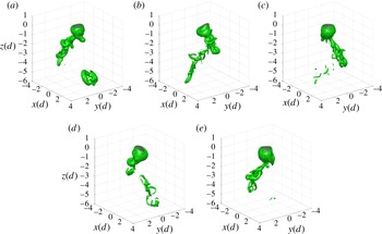
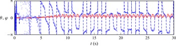
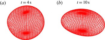
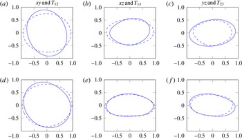
1. Introduction
Significant attention has been devoted to the flow associated with both rigid and fluid particles that are either fixed or freely rising/falling through a continuous phase of a Newtonian fluid. This is due to the relevance of such flows to engineering systems, their common occurrence in geophysical flows, as well as their complex and fascinating nature.
A considerable body of literature addresses the subject of instabilities for fixed, rigid (i.e. non-deformable solid) bodies, freely rising or falling rigid bodies and freely rising or falling fluid particles (gas or liquid). While these systems are related, they differ in the number of degrees of freedom they exhibit and this in turn impacts on the types of instabilities that can occur. In the first case, an instability can only occur in the velocity field around the body. In the second case, in addition to a wake instability, a path instability can also develop. In the last and most complex case, the velocity fields of both phases have to be considered as well as the shape of the deformable interface. In this case, instabilities can be seen in the particle interface in addition to those in the fluid wake and particle trajectory.
The case that is probably best understood is that of a rigid sphere held fixed in a uniform stream, for example in a wind tunnel. Since the numerical work of Natarajan & Acrivos (Reference Natarajan and Acrivos1993), Tomboulides & Orszag (Reference Tomboulides and Orszag2000) and the combined numerical and experimental work of Johnson & Patel (Reference Johnson and Patel1999), a consensus exists that the flow is axisymmetric for Reynolds numbers up to
 $\mathit{Re}\approx 212$
. Axisymmetry is broken by a regular bifurcation and replaced by steady flow with one symmetry plane for
 $\mathit{Re}$
between
 ${\approx}212$
and
 ${\approx}272$
. For Reynolds numbers which are slightly higher, the flow becomes periodic due to a Hopf bifurcation. Finally, periodicity is lost for
 $\mathit{Re}>300$
.
It was established numerically in Jenny, Dusek & Bouchet (Reference Jenny, Dusek and Bouchet2004) that the first, regular bifurcation observed for flow past a fixed sphere is also present in the case of rigid spherical particles rising or falling freely in a quiescent fluid. However, for unconstrained particles, the loss of axisymmetry in the wake at the first bifurcation leads to a lift force that generates oblique particle trajectories. This first bifurcation is weakly dependent on the solid/fluid density ratio
 $\tilde{{\it\rho}}$
. The second bifurcation is only identical to that for a fixed sphere if the density ratio is sufficiently high. Light spheres can attain a regime of in-plane zigzag motion before attaining fully three-dimensional paths, whereas dense spheres develop three dimensionality directly from the oscillatory oblique regime.
This dependence of the rise trajectory after the first bifurcation on the density ratio was experimentally verified in Veldhuis & Biesheuvel (Reference Veldhuis and Biesheuvel2007). Horowitz & Williamson (Reference Horowitz and Williamson2010) further experimentally confirmed these results including the shift to a steady oblique path as a result of the first bifurcation. They further identified a critical density ratio for freely rising spheres: spheres which are sufficiently light (
 $\tilde{{\it\rho}}\leqslant 0.36$
) enter a regime characterized by periodic vibration and a zigzagging trajectory for
 $\mathit{Re}>260$
, where four vortex rings are created per cycle of oscillation; cf. Horowitz & Williamson (Reference Horowitz and Williamson2010). In contrast, denser buoyant spheres remain in the steady oblique regime up to
 $\mathit{Re}=600$
, where an intermittent oblique regime begins. For
 $\mathit{Re}>1550$
, the rise path of the buoyant particles becomes vertical again.
The case of fluid particles, i.e. bubbles and drops, is even more complex due to their deformable interface; see, e.g. Clift, Grace & Weber (Reference Clift, Grace and Weber2005) as a general reference. In addition to the path and wake instabilities observed for rigid particles, bubbles and droplets deform from spherical to ellipsoidal to more general convex shapes, and even to skirted spherical caps. Moreover, their shape can be subject to dynamical changes such as periodic or aperiodic oscillations.
The most common systems for the experimental study of fluid particles are gas bubbles in water. However, such systems are easily influenced by surfactants accumulating at the interface, and the reduced surface mobility can severely influence the bubble dynamics unless extreme care is taken to exclude surfactant effects.
Comprehensive experiments of the dependence of bubble shape on non-dimensional groups such as
 $\mathit{Re}$
,
 $\mathit{Mo}$
and
 $\mathit{Eo}$
(as defined below in (2.30a
), (2.22) and (2.31a
), respectively) can be found in Bhaga & Weber (Reference Bhaga and Weber1981); see Clift et al. (Reference Clift, Grace and Weber2005) for a summary. Concerning the observed particle trajectories, small bubbles rise on rectilinear paths aligned with gravity, whereas larger ones rise on spiral or zigzagging paths (Magnaudet & Eames Reference Magnaudet and Eames2000; Prosperetti Reference Prosperetti2004).
For a long time, there has been speculation as to whether the transition scenario for the wakes of bubbles is qualitatively different from the case of solid spheres. Experiments in ultra-clean water (Duineveld Reference Duineveld1995) have shown, however, that in both cases the route to chaotic behaviour is very similar.
Quantitative information on the wake instabilities of bubbles was obtained through the analyses of Yang & Prosperetti (Reference Yang and Prosperetti2007) and Tchoufag, Magnaudet & Fabre (Reference Tchoufag, Magnaudet and Fabre2013). In those works, a rising bubble was approximated as having an ellipsoidal shape with a free-slip boundary while held fixed in a uniform stream. In a global linear stability analysis, the regular and Hopf wake bifurcations for solid spheres were recovered. However, the stability behaviour depends on more than Reynolds number for the case of free-slip boundaries. A sufficiently large deformation of the bubble shape is necessary for the regular mode to become unstable, as shown in Magnaudet & Mougin (Reference Magnaudet and Mougin2007). The reason for this is that sufficient vorticity must be produced at the bubble surface to trigger the instability. Another striking peculiarity is the fact that, for a given aspect ratio, the flow is only unstable for a finite range of Reynolds numbers. For high enough Reynolds numbers, vorticity is transported away from the interface at a rate sufficient to recover flow stability; see Magnaudet & Mougin (Reference Magnaudet and Mougin2007).
Recently, Cano-Lozano, Bohorquez & Martínez-Bazán (Reference Cano-Lozano, Bohorquez and Martínez-Bazán2013) studied the wake instability using realistic bubble shapes. The bubble shape and rise velocities were determined using steady, axisymmetric volume-of-fluid (VOF) simulations and then fed into a three-dimensional numerical stability analysis of the wake. In the three-dimensional analysis, the bubble interface was modelled as a perfect slip, impermeable boundary of a prescribed and constant shape, held fixed in a uniform liquid stream. Conditions for loss of flow axisymmetry were determined in the aspect ratio-Reynolds number space and found to be influenced by the fore-and-aft symmetry of the bubble – suggesting that the inclusion of realistic bubble shapes is important.
Shape oscillations of gas bubbles in tap water were studied experimentally in Lunde & Perkins (Reference Lunde and Perkins1998). The authors identified three distinct frequencies in their measurements: a vortex shedding frequency, and two frequencies of shape oscillations corresponding to the spherical harmonics of modes (2, 0) and (2, 2). They found that for bubbles of sufficiently large size, the frequencies of the shape oscillations approach the vortex shedding frequency, which was observed to have a constant value of 12 Hz. In Veldhuis, Biesheuvel & Van Wijngaarden (Reference Veldhuis, Biesheuvel and Van Wijngaarden2008), similar experiments were conducted in clean water. There, it was shown that in ultra-clean water, the vortex shedding frequency coincides with the frequency of the (2, 0) mode, and that a deviation from this is caused by the presence of a surfactant.
Concerning the dynamical behaviour of droplets in viscous liquids – as opposed to droplets in a gas phase – there is much less work devoted to rigorous stability and bifurcation analysis. There are several papers (see, e.g. Klee & Treybal Reference Klee and Treybal1956; Schroeder & Kintner Reference Schroeder and Kintner1965; Winnikow & Chao Reference Winnikow and Chao1966; Thorsen, Stordalen & Terjesen Reference Thorsen, Stordalen and Terjesen1968; Greene et al. Reference Greene, Irvine, Gyves and Smith1993 and Abdelouahab & Gatignol Reference Abdelouahab and Gatignol2011) presenting correlations for the terminal drop velocity for falling or rising droplets, several of which also report on oscillatory behaviour for larger droplets. In most of these papers, droplets from organic liquids with viscosities similar to the continuous phase are used, often but not exclusively ascending or settling in water. In the latter case, the typical viscosity ratios are between 0.7 and about 3. Concerning the onset of oscillatory behaviour, qualitative observations are reported such as the decline of the rise velocity for droplets having a Reynolds number above a critical threshold, and the simultaneous occurrence of shape or path oscillations with wake instabilities and vortex shedding. The terminal velocity was found to be somewhat insensitive to droplet viscosity, although shape oscillations were damped with increasing viscosity of the drop. It should be noted that these studies are for pure systems, i.e. efforts were made to avoid artefacts due to contamination that would severely alter the droplet dynamics. Some older work has later been disregarded due to such effects. The influence of a surfactant on the oscillations of oil droplets in water was recently studied in Abi Chebel et al. (Reference Abi Chebel, Vejražka, Masbernat and Risso2012). The oscillations in their experiments were not the result of the hydrodynamics of the rising droplet. Instead, the oscillations were artificially induced by an initial droplet shape that deviated from the spherical case. They found that the presence of surfactant did not change the frequency of the observed oscillations, whereas the damping rates were increased.
There is very little related work on detailed dynamics of higher viscosity oil droplets in water, although the rise behaviour of mineral oil in water is of importance for understanding oil–water separation processes as well as the dispersion of oil from natural oil seeps or artificial oil spills; see, e.g. MacDonald et al. (Reference MacDonald, Leifer, Sassen, Stine, Mitchell and Guinasso2002), Brewer et al. (Reference Brewer, Chen, Warzinski, Baggeroer, Peltzer, Dunk and Walz2006) and North et al. (Reference North, Adams, Schlag, Sherwood, He, Hyun, Socolofsky, Liu, MacFadyen, Ji and Weisberg2011). One exception is the PhD thesis of Haljasmaa (Reference Haljasmaa2006), in which the rise of oil droplets in water has been studied experimentally, with emphasis on instability in the droplet steady rectilinear motion which was shown ‘to correspond to a bifurcation in the drag curve’. Significantly, the onset of this bifurcation did not in general coincide with the onset of vortex shedding around the particle’.
As already mentioned, the oil/water system poses enormous difficulties for experimental study because of problems with contamination, either due to impurities in the oil phase or because of the additives needed to run the experiments. Obviously, such problems are avoided in theoretical studies and therefore the direct numerical simulation of the dynamics of deformable high viscosity droplets in liquids is of particular interest. We are aware of only two references applying such numerical methods in this parameter regime – the PhD thesis of Francois (Reference Francois2002), which uses Immersed Boundary computations, and the paper of Ohta et al. (Reference Ohta, Yamaguchi, Yoshida and Sussman2010), reporting numerical simulations assuming an axisymmetric geometry using a combined Level Set and Volume of Fluid method (CLSVOF). The focus of this latter work is on the influence of the density and viscosity ratios on droplet shape, terminal velocity and break up. As a high viscosity droplet case, a viscosity ratio of 100:1 and a density ratio of 95:100 between dispersed and continuous phase is studied. The range for the Morton number in this study was
 $-5\leqslant \log \mathit{Mo}\leqslant 6$
and the maximum obtained Reynolds number was 100. Note that a higher
 $\mathit{Re}$
would require fully three-dimensional simulations. As demonstrated in Ohta et al. (Reference Ohta, Yamaguchi, Yoshida and Sussman2010), the viscosity ratio is of tremendous importance for the dynamic rise behaviour of bubbles and droplets, but high viscosity droplets have rarely been studied to date.
The case of high viscosity drops in liquids is, in a certain sense, intermediate between the cases of free rigid particles and bubbles: the viscosity almost completely damps out the inner circulation, but the shape can still adjust to the outer forces. The present paper starts the investigation of the dynamical behaviour of such high viscosity droplets as they rise in a quiescent liquid. We focus on the bifurcation cascade which determines the route from almost spherical and vertically rising droplets, via laterally migrating slightly ellipsoidal droplets, to vortex shedding with path and shape oscillations up to almost chaotic shape dynamics and rocking behaviour. We consider as a prototype system the material properties of corn oil droplets in water. This choice is motivated by the PhD thesis of Haljasmaa (Reference Haljasmaa2006), which was supervised by one of the authors (A.M.R.). There, the original motivation for the corn oil/water-system came from studying the dynamics of liquid
 $\text{CO}_{2}$
-droplets in the deep sea as a means of
 $\text{CO}_{2}$
-sequestration; see Metz et al. (Reference Metz, Davidson, de Coninck, Loos and Meyer2005) and cf. Bozzano & Dente (Reference Bozzano and Dente2014) and the references therein concerning the importance of droplet hydrodynamics in this context. The relation to the oil/water system comes from the fact that the density ratio and the dimensionless Morton number, which incorporates only material properties of the involved liquids, is comparable to those of corn and castor oil; see Gangstø, Haugan & Alendal (Reference Gangstø, Haugan and Alendal2005). Indeed, the Morton numbers reported there for oil drops studied in the deep sea in Brewer et al. (Reference Brewer, Peltzer, Friederich and Rehder2002) are in the range
 $9.34\times 10^{-11}$
to
 $1.27\times 10^{-10}$
for droplets at depths of 800–500 m. Corn oil under the conditions considered in Haljasmaa (Reference Haljasmaa2006) resulted in
 $\mathit{Mo}=9\times 10^{-11}$
, while we use
 $\mathit{Mo}=10^{-10}$
in our study; the difference is due to a slightly different water viscosity resulting from different temperatures.
Since we are interested in droplet dynamics from the viewpoint of a bifurcation scenario, with increasingly complex droplet behaviour due to a progressive loss of stability accompanied by the loss of symmetries, we perform fully three-dimensional numerical simulations employing the in-house VOF-code FS3D. We fixed a system of corn oil droplets in water and varied the drop diameter as an input parameter. The main target of this research is a deeper understanding of the different rise characteristics on the route from the rectilinear rise of small droplets to an almost chaotic rise behaviour for large ones. Our study is guided by known results on bubbles (often considered to be of a fixed ellipsoidal shape with slip-boundary conditions) and, at the other extreme, free rigid spheres (with a no-slip boundary condition) rising in water. Particular questions are: (i) do oscillations in shape or path always appear together with wavy wakes and vortex shedding? (ii) Is the steady oblique rise, known for free rigid spheres but apparently not observed for bubbles (cf. Duineveld Reference Duineveld1995 and Wua & Gharib Reference Wua and Gharib2002), attained by oil droplets in water? (iii) As for bubbles, are there regimes of helical, or of zigzagging rise for high viscosity drops?
The remainder of this paper is organized as follows: the governing continuum mechanical equations are stated in the next section and then transformed into their non-dimensional form, where we elaborate on the different roles of the input and output parameters. Section 3 introduces the employed computational technique, the general set-up of the simulations and gives additional information on shape analysis and how integral quantities such as the terminal rise velocity are calculated in general, possibly non-stationary, cases. In § 4, the integral, global quantities obtained from direct numerical simulations for various droplet diameters are presented and analysed concerning prototypical qualitative droplet dynamics. Section 5 then discusses the quantitative behaviour of every simulated droplet with emphasis on instabilities of the path, wake and shape of the droplets. The paper ends with conclusions and an outlook.
2. Mathematical formulation
2.1. Dimensional form of the governing equations
The motion of the droplets is modelled as a two-phase flow, employing continuum physics with the phase boundary represented by a sharp interface. More precisely, we consider isothermal flows of two Newtonian fluids of constant density which are immiscible on the molecular scale. Inside the bulk phases, the incompressibility condition and balance of linear momentum reduce to the Navier–Stokes equations, i.e.
 $$\begin{eqnarray}\displaystyle & \boldsymbol{{\rm\nabla}}\boldsymbol{\cdot }\boldsymbol{v}=0, & \displaystyle\end{eqnarray}$$
 $$\begin{eqnarray}\displaystyle & \partial _{t}({\it\rho}\boldsymbol{v})+\boldsymbol{{\rm\nabla}}\boldsymbol{\cdot }({\it\rho}\boldsymbol{v}\otimes \boldsymbol{v})+\boldsymbol{{\rm\nabla}}p=\boldsymbol{{\rm\nabla}}\boldsymbol{\cdot }\unicode[STIX]{x1D64E}+{\it\rho}\boldsymbol{g} & \displaystyle\end{eqnarray}$$
 $$\begin{eqnarray}\unicode[STIX]{x1D64E}={\it\mu}(\boldsymbol{{\rm\nabla}}\boldsymbol{v}+(\boldsymbol{{\rm\nabla}}\boldsymbol{v})^{\text{T}}).\end{eqnarray}$$
Here,
 $\boldsymbol{v}$
denotes the (local and instantaneous) velocity of the fluid,
 $p$
the mechanical pressure and
 $\boldsymbol{g}$
the acceleration due to gravity. The material parameters of density (
 ${\it\rho}$
) and dynamic viscosity (
 ${\it\mu}$
) are assumed constant, but depend on the respective phase. Whenever distinction between the different phases is necessary,
 $d$
(dispersed) and
 $c$
(continuous) are used as phase indices. So, for example,
 ${\it\Omega}^{d}(t)$
is the time-dependent domain of the liquid droplet, or dispersed phase, while
 ${\it\Omega}^{c}(t)$
is occupied by the ambient liquid, or continuous phase. The interface is denoted by
 ${\it\Sigma}(t)$
and conservation of mass and momentum requires corresponding transmission conditions to hold there. In the present work, we assume a non-contaminated and fully mobile interface. The former corresponds to negligible surface mass densities, i.e. no adsorbed species, while the latter means constant surface tension, i.e. no Marangoni effects due to surface gradients of the surface tension, as well as zero surface viscosities. In this case the surface stress tensor reduces to
 ${\it\sigma}(\unicode[STIX]{x1D644}-\boldsymbol{n}\otimes \boldsymbol{n})$
with constant surface tension
 ${\it\sigma}$
, where
 $\unicode[STIX]{x1D644}$
is the identity matrix and
 $\boldsymbol{n}$
denotes the unit normal at the interface; while the formulas below are invariant under reorientation of the interface, we let
 $\boldsymbol{n}$
point into the dispersed phase. The additional jump conditions read as
 $$\begin{eqnarray}\displaystyle & [\![{\it\rho}(\boldsymbol{v}-\boldsymbol{v}^{{\it\Sigma}})]\!]\boldsymbol{\cdot }\boldsymbol{n}=0, & \displaystyle\end{eqnarray}$$
 $$\begin{eqnarray}\displaystyle & [\![{\it\rho}\boldsymbol{v}\otimes (\boldsymbol{v}-\boldsymbol{v}^{{\it\Sigma}})+p\unicode[STIX]{x1D644}-\unicode[STIX]{x1D64E}]\!]\boldsymbol{\cdot }\boldsymbol{n}={\it\sigma}{\it\kappa}\boldsymbol{n}. & \displaystyle\end{eqnarray}$$
 $\boldsymbol{v}^{{\it\Sigma}}$
is the interfacial velocity and
 ${\it\kappa}$
denotes the curvature – more precisely, the sum of the local principal curvatures – of the interface. The latter is given by
 $$\begin{eqnarray}{\it\kappa}=-\boldsymbol{{\rm\nabla}}_{{\it\Sigma}}\boldsymbol{\cdot }\boldsymbol{n},\end{eqnarray}$$
i.e. minus the surface divergence of the interface normal field. The notation
 $$\begin{eqnarray}[\![{\it\Psi}(t,\boldsymbol{x})]\!]:=\lim _{h\rightarrow 0+}({\it\Psi}(t,\boldsymbol{x}+h\boldsymbol{n})-{\it\Psi}(t,\boldsymbol{x}-h\boldsymbol{n}))\quad \text{for }\boldsymbol{x}\in {\it\Sigma}(t)\end{eqnarray}$$
stands for the jump of a physical quantity
 ${\it\Psi}$
across the interface.
Below, it is assumed that the two-fluid system under consideration does not undergo phase changes. Consequently, the normal component
 $V_{{\it\Sigma}}=\boldsymbol{v}^{{\it\Sigma}}\boldsymbol{\cdot }\boldsymbol{n}$
of the interfacial velocity coincides with the normal component of both the adjacent fluid velocities and, hence, there are no convective fluxes across the interface. Furthermore, since both fluids have non-vanishing viscosity, we suppose that there is no slip between the two phases at the interface. Then, the interfacial jump conditions (2.4), (2.5) simplify to
 $$\begin{eqnarray}[\![\boldsymbol{v}]\!]=0,\quad [\![p\unicode[STIX]{x1D644}-\unicode[STIX]{x1D64E}]\!]\boldsymbol{\cdot }\boldsymbol{n}={\it\sigma}{\it\kappa}\boldsymbol{n}.\end{eqnarray}$$
Separated into normal and tangential parts, the latter condition reads as
 $$\begin{eqnarray}p_{d}-2{\it\mu}_{d}\partial _{\boldsymbol{n}}v_{n}^{d}=p_{c}-2{\it\mu}_{c}\partial _{\boldsymbol{n}}v_{n}^{c}+{\it\sigma}{\it\kappa},\end{eqnarray}$$
where
 $v_{n}=\boldsymbol{v}\boldsymbol{\cdot }\boldsymbol{n}$
and
 $$\begin{eqnarray}{\it\mu}_{d}(\partial _{\boldsymbol{n}}\boldsymbol{v}_{tan}^{d}+\boldsymbol{{\rm\nabla}}_{{\it\Sigma}}v_{n}^{d})={\it\mu}_{c}(\partial _{\boldsymbol{n}}\boldsymbol{v}_{tan}^{c}+\boldsymbol{{\rm\nabla}}_{{\it\Sigma}}v_{n}^{c}),\end{eqnarray}$$
where
 $\boldsymbol{v}_{tan}=\boldsymbol{v}-v_{n}\,\boldsymbol{n}$
is the tangential part of
 $\boldsymbol{v}$
,
 $\partial _{\boldsymbol{n}}$
is the directional derivative into the normal direction and
 $\boldsymbol{{\rm\nabla}}_{{\it\Sigma}}{\it\phi}$
denotes the surface gradient of a quantity
 ${\it\phi}$
. Note that (2.9) reduces to the Young–Laplace equation,
 $$\begin{eqnarray}p_{d}=p_{c}+{\it\sigma}{\it\kappa},\end{eqnarray}$$
in the case of stagnant fluids.
With the discussion of non-dimensionalisation in mind, we prefer to write separate equations for the droplet and the surrounding liquid using a buoyancy formulation. For this purpose we introduce the non-hydrostatic pressure component
 ${\rm\pi}$
as
 $$\begin{eqnarray}{\rm\pi}=p-{\it\rho}_{c}\boldsymbol{g}\boldsymbol{\cdot }\boldsymbol{x}\end{eqnarray}$$
and obtain for the continuous phase the balance of linear momentum in the form
 $$\begin{eqnarray}{\it\rho}_{c}\partial _{t}\boldsymbol{v}+{\it\rho}_{c}(\boldsymbol{v}\boldsymbol{\cdot }\boldsymbol{{\rm\nabla}})\boldsymbol{v}+\boldsymbol{{\rm\nabla}}{\rm\pi}=\boldsymbol{{\rm\nabla}}\boldsymbol{\cdot }\unicode[STIX]{x1D64E}\quad \text{in }{\it\Omega}^{c}(t).\end{eqnarray}$$
For the dispersed phase, the momentum balance takes the form
 $$\begin{eqnarray}{\it\rho}_{d}\partial _{t}\boldsymbol{v}+{\it\rho}_{d}(\boldsymbol{v}\boldsymbol{\cdot }\boldsymbol{{\rm\nabla}})\boldsymbol{v}+\boldsymbol{{\rm\nabla}}{\rm\pi}=\boldsymbol{{\rm\nabla}}\boldsymbol{\cdot }\unicode[STIX]{x1D64E}+({\it\rho}_{d}-{\it\rho}_{c})\boldsymbol{g}\quad \text{in }{\it\Omega}^{d}(t).\end{eqnarray}$$
Considering Newtonian fluids, the viscous stress tensor is
 $$\begin{eqnarray}\unicode[STIX]{x1D64E}=\left\{\begin{array}{@{}ll@{}}{\it\mu}_{c}(\boldsymbol{{\rm\nabla}}\boldsymbol{v}+(\boldsymbol{{\rm\nabla}}\boldsymbol{v})^{\text{T}})\quad \quad & \text{in }{\it\Omega}^{c}(t),\\ {\it\mu}_{d}(\boldsymbol{{\rm\nabla}}\boldsymbol{v}+(\boldsymbol{{\rm\nabla}}\boldsymbol{v})^{\text{T}})\quad \quad & \text{in }{\it\Omega}^{d}(t).\end{array}\right.\end{eqnarray}$$
For a more detailed discussion of the continuum mechanical modelling of two-phase flows see, e.g. Edwards, Brenner & Wasan (Reference Edwards, Brenner and Wasan1991), Ishii & Hibiki (Reference Ishii and Hibiki2011) or Slattery (Reference Slattery1999).
2.2. Non-dimensionalisation of the governing equations
In order to perform the non-dimensionalisation, we first define the dimensionless variables
 $$\begin{eqnarray}\boldsymbol{x}^{\ast }=\boldsymbol{x}/L,\quad t^{\ast }=t/T,\quad \boldsymbol{v}^{\ast }=\boldsymbol{v}/U,\quad p^{\ast }={\rm\pi}/{\rm\pi}_{0},\end{eqnarray}$$
where
 $L,T,U,{\rm\pi}_{0}$
are characteristic values for length, time, velocity and pressure. We also let
 $\boldsymbol{{\rm\nabla}}^{\ast }$
denote the del operator in the dimensionless coordinates. For experiments on freely rising droplets, the droplet volume
 $\mathscr{V}$
is typically an input parameter in the experiments and can be used to define
 $L$
. In particular, we will set
 $L$
equal to
 $d$
, the equivalent spherical diameter of the droplet,
 $$\begin{eqnarray}d=\left(\frac{6\mathscr{V}}{{\rm\pi}}\right)^{1/3}.\end{eqnarray}$$
For freely rising inelastic fluids there is no intrinsic time scale and so we set
 $T=L/U$
. For reference pressure, we set
 ${\rm\pi}_{0}={\it\rho}_{c}U^{2}$
. This is twice the dynamic pressure of the potential flow of an inviscid fluid around a fixed sphere (cf. Clift et al.
Reference Clift, Grace and Weber2005, equation (1)–(32)) at the upper stagnation point. With this choice of
 ${\rm\pi}_{0}$
, the Euler number
 $\mathit{Eu}={\rm\pi}_{0}/{\it\rho}_{c}U^{2}$
is identically one and, hence, will not enter the problem formulation.
In studies of uniform flow past fixed objects, the magnitude of the far-field velocity
 $U_{\infty }$
naturally arises as a prescribed characteristic velocity. For freely moving particles in quasi-steady motion for example, the far-field velocity
 $U_{\infty }$
corresponds to
 $-U_{t}$
, the negative of the (terminal) particle velocity. However, the velocity of freely rising or settling objects is not known a priori, nor is it in general a constant. Therefore,
 $U_{t}$
is defined in terms of the physical parameters of the problem. It follows from the above formulation that the primary physical parameters for freely rising surfactant-free droplets in a quiescent Newtonian medium and in the absence of thermal effects are:
 $$\begin{eqnarray}({\it\rho}_{d},{\it\mu}_{d},\mathscr{V},{\it\rho}_{c},{\it\mu}_{c},{\it\sigma},g).\end{eqnarray}$$
As a consequence of the Buckingham Pi Theorem (see, e.g. Boyling (Reference Boyling1979) for a short proof), there will be four independent dimensionless parameters for this set. Clearly the choice of these independent parameters is not unique. Rather, we select these parameters based on physical considerations. The droplet volume
 $\mathscr{V}$
will not be chosen as a repeating parameter because of its fundamental role in parametric studies for fixed fluid properties. In the limiting case in which the viscous dissipation internal to the drop is negligible, the solution will not depend on
 ${\it\mu}_{d}$
. Furthermore, when the acceleration of the fluid in the droplet is negligible, the droplet density only enters through the term
 ${\rm\Delta}{\it\rho}$
where
 ${\rm\Delta}{\it\rho}={\it\rho}_{c}-{\it\rho}_{d}$
. As can be seen from the above equations, gravity only enters through the product
 ${\rm\Delta}{\it\rho}g$
. With these considerations in mind,
 ${\it\rho}_{c},{\it\mu}_{c}$
and
 ${\rm\Delta}{\it\rho}g$
are chosen as the repeating parameters. We can use them to determine a characteristic velocity,
 $$\begin{eqnarray}U=\left(\frac{{\it\mu}_{c}{\rm\Delta}{\it\rho}g}{{\it\rho}_{c}^{2}}\right)^{1/3},\end{eqnarray}$$
and also to define the following dimensionless groups
 $$\begin{eqnarray}\tilde{{\it\rho}}={\it\rho}_{d}/{\it\rho}_{c},\quad \tilde{{\it\mu}}={\it\mu}_{d}/{\it\mu}_{c},\quad \tilde{\mathscr{V}}=\mathscr{V}\,\frac{{\rm\Delta}{\it\rho}g{\it\rho}_{c}}{{\it\mu}_{c}^{2}},\quad \tilde{{\it\sigma}}={\it\sigma}\left(\frac{{\it\rho}_{c}^{2}}{{\it\mu}_{c}^{4}{\rm\Delta}{\it\rho}g}\right)^{1/3}.\end{eqnarray}$$
Employing the equivalent spherical diameter
 $d$
from (2.17), it follows that
 $\tilde{\mathscr{V}}$
is proportional to a generalisation of the Archimedes number used in Karamanev, Chavarie & Mayer (Reference Karamanev, Chavarie and Mayer1996) for rigid spheres,
 $$\begin{eqnarray}\mathit{Ar}=\frac{{\rm\Delta}{\it\rho}g\,{\it\rho}_{c}\,d^{3}}{{\it\mu}_{c}^{2}}.\end{eqnarray}$$
This in turn is the square of the Galileo number
 $G$
used in Jenny et al. (Reference Jenny, Dusek and Bouchet2004). Clearly, the Archimedes number can also be viewed as a dimensionless volume or, alternatively, as a measure of buoyancy to viscous effects. The parameter
 $\tilde{{\it\sigma}}$
is the inverse of the Morton number (
 $\mathit{Mo}$
) raised to the one third power, i.e.
 $$\begin{eqnarray}\mathit{Mo}=\frac{{\it\mu}_{c}^{4}{\rm\Delta}{\it\rho}g}{{\it\rho}_{c}^{2}{\it\sigma}^{3}}.\end{eqnarray}$$
Notably, the Morton number depends only on material parameters and the acceleration due to gravity and is independent of the droplet geometry. Without loss of generality, we can then represent our complete set of dimensionless parameters as
 $$\begin{eqnarray}(\tilde{{\it\rho}},\tilde{{\it\mu}},\mathit{Ar},\mathit{Mo}).\end{eqnarray}$$
After substituting the definitions for
 $L,U,T$
and
 ${\rm\pi}_{0}$
in (2.1)–(2.2) and (2.4)–(2.5), and organising the parameters into the dimensionless groups (2.23), we obtain the non-dimensional form of the two-phase Navier–Stokes system, i.e.
 $$\begin{eqnarray}\displaystyle & \boldsymbol{{\rm\nabla}}^{\ast }\boldsymbol{\cdot }\boldsymbol{v}^{\ast }=0\quad \text{in }{\it\Omega}\setminus {\it\Sigma}, & \displaystyle\end{eqnarray}$$
 $$\begin{eqnarray}\displaystyle & \displaystyle \partial _{t^{\ast }}\boldsymbol{v}^{\ast }+(\boldsymbol{v}^{\ast }\boldsymbol{\cdot }\boldsymbol{{\rm\nabla}}^{\ast })\boldsymbol{v}^{\ast }+\boldsymbol{{\rm\nabla}}^{\ast }p^{\ast }=\frac{1}{\mathit{Ar}^{1/3}}{\it\Delta}^{\ast }\boldsymbol{v}^{\ast }\quad \text{in }{\it\Omega}_{c}, & \displaystyle\end{eqnarray}$$
 $$\begin{eqnarray}\displaystyle & \displaystyle \tilde{{\it\rho}}\partial _{t^{\ast }}\boldsymbol{v}^{\ast }+\tilde{{\it\rho}}(\boldsymbol{v}^{\ast }\boldsymbol{\cdot }\boldsymbol{{\rm\nabla}}^{\ast })\boldsymbol{v}^{\ast }+\boldsymbol{{\rm\nabla}}^{\ast }p^{\ast }=\frac{\tilde{{\it\mu}}}{\mathit{Ar}^{1/3}}{\it\Delta}^{\ast }\boldsymbol{v}^{\ast }-\mathit{Ar}^{1/3}(1-\tilde{{\it\rho}})\boldsymbol{e}_{g},\quad \text{in }{\it\Omega}_{d}, & \displaystyle\end{eqnarray}$$
 $$\begin{eqnarray}\displaystyle & [\![\boldsymbol{v}^{\ast }]\!]=0\quad \text{at }{\it\Sigma}, & \displaystyle\end{eqnarray}$$
 $$\begin{eqnarray}\displaystyle & \displaystyle [\![p^{\ast }]\!]\,\boldsymbol{n}-\frac{1}{\mathit{Ar}^{1/3}}[\![\tilde{\unicode[STIX]{x1D64E}}]\!]\boldsymbol{\cdot }\boldsymbol{n}=\frac{\tilde{{\it\kappa}}}{\mathit{Mo}^{1/3}\,\mathit{Ar}^{1/3}}\boldsymbol{n}\quad \text{at }{\it\Sigma}, & \displaystyle\end{eqnarray}$$
 $\boldsymbol{e}_{z}=\boldsymbol{g}/\Vert \boldsymbol{g}\Vert$
,
 $\tilde{{\it\kappa}}={\it\kappa}d$
and
 $\tilde{\unicode[STIX]{x1D64E}}=\unicode[STIX]{x1D64E}/({\it\rho}U^{2})$
.
2.3. Non-dimensional form of the output variables
Depending on the imposed conditions, freely rising particles may approach a stationary or a periodic terminal state, or show non-periodic behaviour for arbitrarily large periods of time. In any case, we define a terminal rise velocity
 $U_{t}$
by averaging over a sufficiently long time scale. This velocity is a result of the imposed conditions. For details on how the terminal rise velocity is determined for non-steady droplets, see § 4. We further consider characteristic frequencies
 $f$
that may be used to describe the motion or surface deformation of the droplet.
Using the same parameters (2.18), we define a dimensionless velocity
 $\tilde{U} _{t}$
and a dimensionless frequency
 $\tilde{f}$
as
 $$\begin{eqnarray}\tilde{U} _{t}=U_{t}\left(\frac{{\it\rho}_{c}^{2}}{{\it\mu}_{c}{\rm\Delta}{\it\rho}g}\right)^{1/3},\quad \tilde{f}=f\left(\frac{{\it\rho}_{c}{\it\mu}_{c}}{{\rm\Delta}{\it\rho}^{2}g^{2}}\right)^{1/3}.\end{eqnarray}$$
In studies of uniform flow past fixed objects, the magnitude of the far-field velocity
 $U_{\infty }$
naturally arises as a characteristic velocity, and the drag force and the frequency of vortex shedding are measured as a function of this parameter. This data is then presented with respect to the functional dependence of the drag coefficient (
 $C_{D}$
) and Strouhal (
 $\mathit{St}$
) number on Reynolds number (
 $\mathit{Re}$
). Historically, these parameters have continued to be used for freely rising rigid particles, despite the fact that the velocity of the rising particle is unknown a priori and will not in general be constant. For this reason, we recall the relationships between
 $\mathit{Re},C_{D},\mathit{St}$
and the groups (2.23), namely
 $$\begin{eqnarray}\mathit{Re}=\frac{{\it\rho}_{c}U_{t}d}{{\it\mu}_{c}}=Ar^{1/3}\tilde{U} _{t},\quad C_{D}=\frac{4}{3}\frac{{\rm\Delta}{\it\rho}gd}{{\it\rho}_{c}U_{t}^{2}}=\frac{4}{3}\frac{\mathit{Ar}^{1/3}}{\tilde{U} _{t}^{2}},\quad \mathit{St}=\frac{fd}{U_{t}}=\mathit{Ar}^{1/3}\frac{\tilde{f}}{\tilde{U} _{t}}.\end{eqnarray}$$
Note that we build the Reynolds number on the droplet diameter as in Clift et al. (Reference Clift, Grace and Weber2005); several other authors use the droplet radius instead. It should also be noted that the representation of
 $C_{D}$
in (2.30) does not apply to the flow around fixed solid particles, since the buoyancy force is irrelevant for fixed particles. Recall that in the general case, the drag coefficient is defined as
 $C_{D}=(8F_{D}/{\rm\pi}{\it\rho}_{c}U_{t}^{2}d^{2})$
with
 $F_{D}$
denoting the drag force.
The role of surface tension relative to buoyancy and inertial effects is sometimes considered through the Eótvòs number (also called the Bond number) and Weber number, respectively defined as
 $$\begin{eqnarray}\mathit{Eo}=\frac{{\rm\Delta}{\it\rho}\;g\;d^{2}}{{\it\sigma}}=\mathit{Mo}^{1/3}Ar^{2/3},\quad \mathit{We}=\frac{{\it\rho}_{c}U_{t}^{2}d}{{\it\sigma}}=\mathit{Mo}^{1/3}Ar^{-1/3}\mathit{Re}^{2}.\end{eqnarray}$$
3. Numerical method
3.1. Volume of fluid method
All numerical simulations in this work have been performed with the finite volume based in-house code Free Surface 3D, originally developed by Rieber (Reference Rieber2004). The position of the interface is tracked using the VOF method of Hirt & Nichols (Reference Hirt and Nichols1981). The fluxes of the volume fraction function are determined geometrically, employing the Piecewise Linear Interface Calculation (PLIC) algorithm of Rider & Kothe (Reference Rider and Kothe1998). Surface tension is treated by the Continuum Surface Force model (Brackbill, Kothe & Zemach Reference Brackbill, Kothe and Zemach1992), in a so-called balanced force implementation (Renardy & Renardy Reference Renardy and Renardy2002) where curvature information is calculated by the height function algorithm described in Popinet (Reference Popinet2009). This has been extensively validated within FS3D for falling films, see Albert, Raach & Bothe (Reference Albert, Raach and Bothe2012). In order to correctly capture the coupling of tangential stresses at the free surface, a combination of arithmetic and harmonic averaging of viscosities in the interface cells as introduced in Tryggvason et al. (Reference Tryggvason, Bunner, Ebrat and Tauber1998) is used.
The VOF-solver employed here is able to handle realistic viscosity and density ratios. FS3D is well validated for droplets impinging on wetted surfaces (Rieber & Frohn Reference Rieber and Frohn1999), for binary droplet collisions (e.g. Gotaas et al. Reference Gotaas, Havelka, Jakobsen, Svendsen, Hase, Roth and Weigand2007; Focke & Bothe Reference Focke and Bothe2012 and Focke et al. Reference Focke, Kuschel, Sommerfeld and Bothe2013), rising bubbles in water and water–glycerol mixtures (Koebe, Bothe & Warnecke Reference Koebe, Bothe and Warnecke2003; Bothe, Schmidtke & Warnecke Reference Bothe, Schmidtke and Warnecke2006) and several other two-phase flows with additional transport processes, in particular mass transfer (Bothe & Fleckenstein Reference Bothe and Fleckenstein2013; Fleckenstein & Bothe Reference Fleckenstein and Bothe2013; Weirich, Köhne & Bothe Reference Weirich, Köhne and Bothe2014), thermocapillary flow (Ma & Bothe Reference Ma and Bothe2011) and evaporation (Ma & Bothe Reference Ma and Bothe2013).
For diffusive momentum transport, the explicit Euler method is used, which imposes a stability constraint on the time step according to
 $$\begin{eqnarray}{\rm\Delta}t\leqslant \frac{({\rm\Delta}x)^{2}}{2\max \{{\it\mu}_{d}/{\it\rho}_{d},{\it\mu}_{c}/{\it\rho}_{c}\}}\end{eqnarray}$$
where
 ${\rm\Delta}x$
denotes the grid width. Because of this limitation, the application of FS3D to oil drops in water proved to be challenging, since typical oil viscosities greatly exceed the viscosity of water: for the corn oil used in the simulations, the viscosity ratio
 $\tilde{{\it\mu}}$
is 45. Such high fluid viscosities imply fast diffusion of momentum and therefore require small time steps in the simulations. Other time step constraints need to be respected in the simulations, most notably the CFL condition. However, in all simulation runs in the present work, condition (3.1) was the limiting one. In all simulations,
 ${\rm\Delta}t$
was set to 0.75 times the maximal allowed value. A further reduction of the time step did not have a noticeable effect on the simulation results.
3.2. Set-up for VOF-simulations
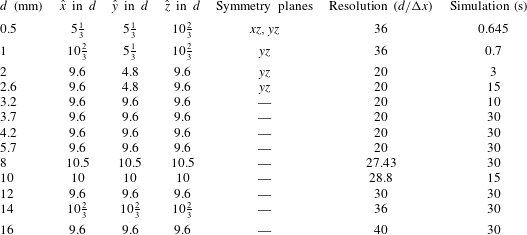
All computations were performed for a box-shaped computational domain of size
 $(0,\hat{x})\times (0,{\hat{y}})\times (0,\hat{z})$
. The simulation of the smallest droplet with a diameter of 0.5 mm was performed with two symmetry planes, which means that effectively only a quarter of a droplet was simulated. The 1 and 2 mm simulations were performed with a single symmetry plane, corresponding to the computation of half a droplet. All larger droplet sizes were simulated without symmetry.
Gravitational acceleration was aligned with the negative
 $z$
direction; due to buoyancy, the droplets therefore rose in the positive
 $z$
direction. To reduce the influence of the wall on drop movement, slip boundary conditions were prescribed on the lateral walls and on the boundary in the positive
 $z$
direction. In the negative
 $z$
direction, a continuous (outlet) boundary condition was used in order to let perturbations in the droplet wake leave the computational domain smoothly. Pressure was determined using the buoyancy formulation (2.13) and (2.14).
The computational domain was moved with the droplet barycentre such that it stayed within one cell of its initial position. As soon as the barycentre crossed the boundary of a cell, the arrays describing the current state of the simulation were copied back one layer, effectively ensuring that the barycentre of the droplet never deviates more than
 ${\rm\Delta}x$
from its initial position.
Due to the different physical phenomena for droplets of different sizes, it was not possible to use the same computational set-up for all simulations. Instead, the resolution had to be adapted on a case by case basis. Very small droplets required a high resolution in order to limit the influence of so-called parasitic currents, i.e. artificial velocity fluctuations close to the droplet surface due to numerical errors in the normal and curvature computations, which can be severe for the high curvatures encountered at small droplet diameters. Very large droplets show almost chaotic behaviour, and thus a sufficiently high resolution is needed to adequately resolve their complex velocity fields.
All computational domains had a size of at least
 $(0,9.6d)\times (0,9.6d)\times (0,9.6d)$
. FS3D solves the pressure Poisson equation using the geometrical multigrid approach, for which it is advantageous if the prime factorisation of the resolution in each direction contains a large power of two. Therefore, it was often computationally more efficient to choose a slightly larger domain. Drop shapes and terminal rise velocities do not significantly differ if the wall distance is increased, cf. table 3. Table 1 displays all domain sizes and resolutions used in the present work.
Size of computational domain, number of symmetry planes, resolution and simulation time for the different simulation runs.

The simulations are initialised with spherical oil drops released in stagnant water. For simulations without symmetry, the initial centre of the droplet was set to
 $(1/2\hat{x},1/2{\hat{y}},2/3\hat{z})$
; otherwise, the droplet centre was set to be on the symmetry plane. In test runs initialised with oblate ellipsoid shapes (drop width larger than the height), the resulting terminal velocity and aspect ratio are unchanged.
The employed material parameters and derived dimensionless numbers are given in table 2.
Material parameters used in the simulations and values of dimensionless numbers that depend solely on these parameters.

3.3. Grid independence studies
As will be discussed below, the dynamic behaviour of the droplet changes qualitatively over the large range of droplet sizes considered here. Accordingly, adequately capturing the flow physics requires very different numerical resolutions. For the smaller droplets, the interfacial curvature is high, leading to problems in correctly capturing surface tension effects. For the smallest droplets with a diameter of 0.5 mm, analytic solutions were used to confirm the adequacy of the mesh density; see § 5.1.3. A simulation with a coarser grid (18 cells per diameter) did exhibit instabilities for the terminal velocities due to parasitic currents. For a higher resolution (72 cells per diameter) however, the computation time considerably increases; on 250 cores, the estimated run time is roughly seven months.
For the 2 mm droplet, the difference in terminal rise velocity between simulations with a resolution of 16 cells per droplet diameter and simulations with 26.7 cells per droplet diameter was less than 3 %, so it was decided that a resolution of 20 cells was sufficient. The simulation with the somewhat lower spatial resolution was chosen for the present study, because longer physical time intervals become accessible then.
For larger droplets, the behaviour becomes more and more chaotic, and a true grid independence of the simulation results cannot be achieved. Concerning the influence of wall effects, as can be seen from table 3, a double lateral domain size affects the terminal rise velocity for the 5.7 mm droplets by 0.8 %.
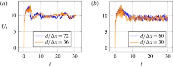
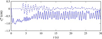
Rise velocity in
 $\text{cm}~\text{s}^{-1}$
over time in s for 14 mm (a) and 16 mm (b) droplet.

Integral quantities for 5.7 mm droplet for simulations with different resolutions and domain size (
 $U_{t}$
in
 $\text{cm}~\text{s}^{-1}$
, DLS: double lateral domain size).

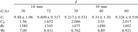
Integral quantities for 14 and 16 mm droplets for simulations with different resolutions (
 $U_{t}$
in
 $\text{cm}~\text{s}^{-1}$
).

Nevertheless, even for the largest droplet, a simulation with a resolution of only 30 cells per droplet diameter results in a terminal rise velocity that differs by less than 1 % from the value achieved with a resolution of 40 cells. Likewise, the deviation of the terminal velocity for a resolution of 60 cells per diameter is less than 0.1 %, cf. table 4. Figure 1 depicts the time evolution of the rise velocities for the 14 and 16 mm droplets for different resolutions. For the 14 mm droplets, increasing the resolution slightly shifts the peak velocity to earlier times, while the global qualitative appearance is retained. For the 16 mm droplets, an increased resolution reduces the amplitude of the velocity oscillations within the acceleration phase and smoothes the transition to the stationary phase. But the qualitative rise behaviour described later is already captured at the relatively moderate resolution of 30 cells per diameter, and the reported vortex shedding frequency also does not significantly differ. However, for the very long physical simulation times required to determine the behaviour of the droplets at large times, small numerical errors in mass conservation can accumulate. In order to keep total mass errors small, the relatively high resolution of 40 cells per diameter had to be chosen. The overall error in droplet mass was, for all simulations, less than 2 % which corresponds to an error in radius of less than 0.65 %.
3.4. Shape analysis
From the direct numerical simulations in FS3D, we obtain a sample set of points, which we denote
 $\unicode[STIX]{x1D653}=[\boldsymbol{x}_{1},\dots ,\boldsymbol{x}_{N}]$
. Its elements
 $\boldsymbol{x}_{i}\in \mathbb{R}^{3}$
are obtained as the intersections of the PLIC surfaces and the edges of the computation cells, where we have applied a spherical layer filtering to remove numerical wisps. Note also that the rows of
 $\unicode[STIX]{x1D653}$
have zero mean. Resorting to this sample set, the goal is to compute an approximate interface
 $\bar{{\it\Sigma}}$
in terms of a power series, ensuring conservation of volume for the fluid phases. With this objective, spherical coordinates, i.e.
 $$\begin{eqnarray}{\it\Sigma}=\left\{R\cdot \left[\cos {\it\varphi}\sin {\it\theta},\sin {\it\varphi}\sin {\it\theta},\cos {\it\theta}\right]^{\text{T}}:({\it\varphi},{\it\theta})\in [0,2{\rm\pi})\times [0,{\rm\pi}]\right\},\end{eqnarray}$$
appear to be an appropriate choice. However, the convergence properties of the expansion of the radius
 $R({\it\varphi},{\it\theta})$
in terms of real spherical harmonics
 $Y_{l}^{m}$
crucially depend on the interface shape. In the vicinity of the smallest sphere entirely enclosing the interface, the expansion converges quickly. However, for general aspherical bodies, the convergence of spherical harmonic series within the so-called Brillouin sphere is more complicated. For an ellipsoidal surface with semi-axes
 $a>b>c>0$
, Pick, Picha & Vyskocil (Reference Pick, Picha and Vyskocil1973) and Balmino (Reference Balmino1994) have shown that convergence of the spherical harmonic series requires the semi-axes of the ellipsoid to satisfy
 $a>b>c>a/\sqrt{2}$
, corresponding to a maximum aspect ratio of
 $1/\sqrt{2}$
. Since in the context of this work, the previously stated condition is too restrictive, some modifications, including an ellipsoid compression, are necessary, which are introduced in the next section. Subsequently, we give a brief introduction to shape description using bi-ellipsoids and spherical harmonics decomposition.
3.4.1. Principal component analysis and ellipsoid compression
The principal axes
 $\unicode[STIX]{x1D64F}_{PA}=[\boldsymbol{t}_{1},\boldsymbol{t}_{2},\boldsymbol{t}_{3}]$
with
 $\Vert \boldsymbol{t}_{i}\Vert =1$
of the droplet can be computed as the eigenvectors of the symmetric matrix
 $\unicode[STIX]{x1D63C}:=\unicode[STIX]{x1D653}^{\text{T}}\unicode[STIX]{x1D653}$
, where we assume that the associated eigenvalues
 ${\it\tau}_{i}$
fulfill
 ${\it\tau}_{1}\geqslant {\it\tau}_{2}\geqslant {\it\tau}_{3}$
. Since we expect the droplet to flatten, i.e. stretch in the lateral direction, the smallest eigenvalue of
 $\unicode[STIX]{x1D63C}$
, i.e.
 ${\it\tau}_{3}$
, indicates the direction of rise. Figure 35 exemplifies interface sections in Cartesian and principal coordinates. For the above mentioned ellipsoid compression, we transform
 $\unicode[STIX]{x1D653}$
to the principal coordinate system, i.e.
 $\unicode[STIX]{x1D653}_{PA}:=\unicode[STIX]{x1D64F}_{PA}^{\text{T}}\unicode[STIX]{x1D653}$
. The semi axes
 $\{a_{CE},b_{CE},c_{CE}\}$
of the compression ellipsoid, which are assumed to align to the principal axes, are then obtained from an LSE fit. Finally, we transform the set points according to
 $\unicode[STIX]{x1D653}_{PA}^{\ast }:=\text{diag}\,\{a_{CE}^{-1},b_{CE}^{-1},c_{CE}^{-1}\}\boldsymbol{\cdot }\unicode[STIX]{x1D64F}_{PA}^{\text{T}}\unicode[STIX]{x1D653}$
to perform the spherical harmonics decomposition.
3.4.2. Bi-ellipsoid shape description
As a bi-ellipsoid we define a composition of two half-ellipsoids which share two equatorial semi-axes
 $a,b$
, but have different sagittal semi-axes
 $c^{\pm }$
. The surface is then implicitly given by
 ${\it\Sigma}=\{\boldsymbol{x}\in \mathbb{R}^{3}:{\it\phi}(\boldsymbol{x})=0\}$
, where
 ${\it\phi}$
is the level set function
 $$\begin{eqnarray}{\it\phi}\left(\boldsymbol{x}\right)=\frac{x^{2}}{a^{2}}+\frac{y^{2}}{b^{2}}+\frac{z^{2}}{[c(z)]^{2}}-1\quad \text{with }c(z)=\left\{\begin{array}{@{}ll@{}}c^{+}\quad & z>0\\ c^{-}\quad & z\leqslant 0.\end{array}\right.\end{eqnarray}$$
The curvature is discontinuous at the equatorial plane and can be computed as the negative surface divergence of the unit normal, i.e.
 ${\it\kappa}:=-\boldsymbol{{\rm\nabla}}_{{\it\Sigma}}\boldsymbol{\cdot }\boldsymbol{n}$
with
 $\boldsymbol{n}:=(\boldsymbol{{\rm\nabla}}{\it\phi}/\Vert \boldsymbol{{\rm\nabla}}{\it\phi}\Vert )$
. But note that due to the discontinuity of the level set function, an analytical solution to the least squares minimization problem is not feasible. Thus, the estimation of the parameter set
 $\{a,b,c^{+},c^{-}\}$
from the transformed sample set
 $\unicode[STIX]{x1D653}_{PA}$
is conducted as follows. The equatorial semi-axes
 $a,b$
are assumed to coincide with those of the ellipsoid compression, i.e.
 $a:=a_{CE}$
and
 $b:=b_{CE}$
. The sagittal semi-axes
 $c^{\pm }$
are computed to pertain the total height and droplet centre of mass, i.e.
 $z_{max}-z_{0}=c^{+}$
and
 $-z_{min}+z_{0}=c^{-}$
with
 $z_{0}=3/8\left(c^{-}-c^{+}\right)$
.
Due to the discontinuity of the sagittal semiaxis
 $c$
, the direct computation of the curvature will exhibit an unphysical jump at the equatorial plane. To overcome this, we also introduce a smoothed transition for
 $c$
in (3.3), namely
 $$\begin{eqnarray}c(z)=c^{+}+\frac{c^{-}-c^{+}}{{\rm\pi}}\left(\arctan (-kz)+\frac{{\rm\pi}}{2}\right),\end{eqnarray}$$
where
 $k>0$
controls the width of the transition region. The aspect ratio of a bi-ellipsoid is defined as
 $$\begin{eqnarray}{\it\alpha}(t):=\frac{c^{+}(t)+c^{-}(t)}{2\sqrt{a(t)b(t)}}.\end{eqnarray}$$
3.4.3. Spherical harmonics decomposition
Spherical harmonics form an orthonormal basis on the unit sphere and are thus an appropriate tool for the representation of star-shaped surfaces embedded in
 $\mathbb{R}^{3}$
, cf. figure 34 for a prototypical droplet interface reconstructed from spherical harmonics. For a treatise on spherical harmonics analysis, see, cf. Tsoulis (Reference Tsoulis1999). To obtain the coefficients
 $c_{l}^{m}$
, we minimize the error
 $$\begin{eqnarray}\mathscr{E}=\frac{1}{2}\mathop{\sum }_{i=1}^{N}\left(R_{i}-\mathop{\sum }_{m=0}^{L}\mathop{\sum }_{l=-m}^{m}c_{l}^{m}Y_{l}^{m}\left({\it\varphi}_{i},{\it\theta}_{i}\right)\right)^{2},\end{eqnarray}$$
with
 $R_{i}:=\Vert \boldsymbol{x}_{i}\Vert$
,
 ${\it\varphi}_{i}:=\arctan y_{i}/x_{i}$
,
 ${\it\theta}_{i}:=\arccos z_{i}/R_{i}$
and the real spherical harmonics
 $$\begin{eqnarray}Y_{l}^{m}\left({\it\varphi},{\it\theta}\right)=\left\{\begin{array}{@{}ll@{}}\displaystyle \sqrt{2}\sqrt{\frac{2l+1}{4{\rm\pi}}\frac{\left(l+m\right)!}{\left(l-m\right)!}}P_{l}^{-m}\left(\cos {\it\theta}\right)\sin \left(-m{\it\varphi}\right) & \text{if }m<0\\ \displaystyle \sqrt{\frac{2l+1}{4{\rm\pi}}}P_{l}^{m}\left(\cos {\it\theta}\right) & \text{if }m=0\\ \displaystyle \sqrt{2}\sqrt{\frac{2l+1}{4{\rm\pi}}\frac{\left(l-m\right)!}{\left(l+m\right)!}}P_{l}^{m}\left(\cos {\it\theta}\right)\cos m{\it\varphi} & \text{if }m>0,\end{array}\right.\end{eqnarray}$$
where
 $P_{l}^{m}$
stands for the associated Legendre polynomial. Note that we do not include the Condon-Shortley phase, i.e. the pre-factor
 $\left(-1\right)^{m}$
, in the definition of the spherical harmonics. The resulting LSE problem can be cast in matrix form as
 $$\begin{eqnarray}\unicode[STIX]{x1D654}\unicode[STIX]{x1D654}^{\text{T}}\boldsymbol{c}=\unicode[STIX]{x1D654}\boldsymbol{r}\end{eqnarray}$$
with the multi-index
 $\boldsymbol{k}:=\left(l,m\right)$
and
 $\boldsymbol{r}=R_{i}\boldsymbol{e}_{i},~\unicode[STIX]{x1D654}=Y_{\boldsymbol{k}_{j}}\left({\it\varphi}_{i},{\it\theta}_{i}\right)\boldsymbol{\cdot }\left(\boldsymbol{e}_{i}\otimes \boldsymbol{e}_{j}\right),~\boldsymbol{c}=c_{\boldsymbol{k}_{j}}\boldsymbol{e}_{j}\text{ for }i\in [1,N],j\in [1,\left(L+1\right)^{2}]$
. Note that in the context of this work it holds that
 $N\gg \left(L+1\right)^{2}$
.
3.5. Calculation of integral quantities
The velocity data was determined in the following way: for every time step, the centre of mass of the droplet was determined as
 $$\begin{eqnarray}\boldsymbol{x}_{COM}=\frac{1}{\mathscr{V}}\int _{{\it\Omega}_{d}(t)}\boldsymbol{x}\,\text{d}\boldsymbol{x}.\end{eqnarray}$$
For the first and last time step, the velocity
 $\boldsymbol{v}$
was then calculated by forward or backward differencing, respectively, and by central differences for all other times.
The terminal rise velocity was determined as
 $$\begin{eqnarray}U_{t}=\frac{1}{t_{2}-t_{1}}\left|\int _{t_{1}}^{t_{2}}\boldsymbol{v}\boldsymbol{\cdot }\boldsymbol{e}_{z}\,\text{d}{\it\tau}\right|,\end{eqnarray}$$
where
 $t_{2}$
is the simulation time according to table 1, and
 $t_{1}$
is the time after which the (qualitatively) final state is reached. The latter time is given in table 5. All the simulation times are sufficiently long, so that reliable mean values are obtained even for droplets whose final state is unsteady. The lateral velocities
 $U_{x}$
,
 $U_{y}$
are defined analogously to
 $U_{t}$
, the deviations correspond to the respective RMS.
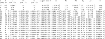
Results for integral quantities.

4. Results for integral quantities
For each droplet diameter listed in table 1, a direct numerical simulation has been performed from which the terminal velocity
 $U_{t}$
, the lateral velocities
 $U_{x}$
and
 $U_{y}$
as well as the aspect ratio, together with their RMS values, have been extracted by calculations as explained in §§ 3.4 and 3.5. These values were obtained from data after time
 $t_{1}$
, which is also displayed in table 1, when the droplets reached their final state. Depending on the large-time behaviour of the droplet,
 $t_{1}$
is either defined as the time when a steady terminal velocity is reached, when time-periodic behaviour is reached or when a non-periodic behaviour is present that does not change qualitatively anymore. From these basic integral quantities and the material parameters in table 2, the above defined non-dimensional numbers
 $\mathit{Ar}$
,
 $\mathit{Re}$
,
 $\mathit{We}$
,
 $\mathit{Eo}$
,
 $G$
and the non-dimensional drag
 $C_{D}$
are computed. All these basic outcomes of the simulation runs are listed in table 5.
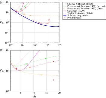
Figure 3 displays the dependence of the drag coefficient
 $C_{D}$
on
 $\mathit{Re}$
for the present study, together with other drag curves including the standard drag curve for fixed solid spheres. For the liquid drops considered here, the drag coefficient initially decreases with
 $\mathit{Re}$
, until a minimum is reached at about
 $\mathit{Re}=1000$
. For higher Reynolds numbers, the drag experiences a sharp increase, accompanied by the onset of shape oscillations. This is in accordance with Harper (Reference Harper1972), where a distinction is made between high and low Morton number fluids. For the former, the drag coefficient decreases monotonically with the Reynolds number, whereas for the latter a minimum of
 $C_{D}$
exists. Bhaga & Weber (Reference Bhaga and Weber1981) placed the separating value at
 $\mathit{Mo}=4\times 10^{-3}$
. The Morton number encountered in this work is much smaller than that and, accordingly, a minimum of
 $C_{D}$
is to be expected.
Note that the minimum drag among the simulated droplets is attained at
 $\mathit{We}=4.50$
, followed by a sharp increase in the drag. This is consistent with estimates for the critical Weber number for droplets, which is 4.04 in Winnikow & Chao (Reference Winnikow and Chao1966). Slightly differing values from other sources are compiled in the recent overview (Wegener, Paul & Kraume Reference Wegener, Paul and Kraume2014) on droplet fluid dynamics. In Winnikow & Chao (Reference Winnikow and Chao1966), the authors report that drop oscillations and changes in the wake structure set in at
 $\mathit{We}=4$
, Greene et al. (Reference Greene, Irvine, Gyves and Smith1993) mention the onset of droplet oscillations; these papers study falling droplets in liquids.
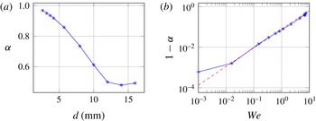
In our simulations, for Weber numbers above 4, significant deformations of the droplets are observed. Since the Weber number resembles the ratio of inertia to surface tension forces, it is interesting to visualize the aspect ratio as a function of
 $\log _{10}\mathit{We}$
. This is depicted in figure 4, which also shows the aspect ratio against the droplet diameter. A linear regression between
 $\log _{10}{\it\alpha}$
and
 $\log _{10}\mathit{We}$
, cf. the dashed line in the right panel of figure 4, yields the relation
 $$\begin{eqnarray}{\it\alpha}\approx 1-0.0773\mathit{We}^{0.92},\end{eqnarray}$$
where the 0.5 mm droplet was disregarded. The 8 mm droplet has a mean aspect ratio of 0.735 at a Weber number of
 $\mathit{We}=4.50$
. Interestingly, the data shows a minimum mean aspect ratio for the 14 mm droplet.
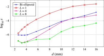
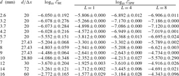
Shape error as a function of droplet diameter in mm. Note that the order
 $L$
of the spherical harmonics implies
 $\left(L+1\right)^{2}$
coefficients; cf. table 7.

(a) Drag curves from Proudman & Pearson (Reference Proudman and Pearson1957) (orange: first order in
 $\mathit{Re}$
, green: second order in
 $\mathit{Re}$
), Goldstein (Reference Goldstein1929) (magenta, fifth order in
 $\mathit{Re}$
), Taylor & Acrivos (Reference Taylor and Acrivos1964) (red, cf. (5.1)), Chester & Breach (Reference Chester and Breach1969) (pink) and standard drag curve (blue) for solid spheres from Clift et al. (Reference Clift, Grace and Weber2005) compared with DNS results (○: present study) and roots of (5.3) (
 $\times$
: 0.5 mm, ▫: 1 mm, ▵: 2 mm). (b) close-up for
 $\mathit{Re}<20$
.

Mean aspect ratio of bi-ellipsoid as a function of diameter in mm (a) and Weber number ((b),
 $\mathit{We}=({\it\rho}_{c}\,\text{d}U_{t}^{2})/{\it\sigma}$
) with linear regression (dashed,
 $(\mathit{We}=10^{-3},{\it\alpha}=0.999)$
was omitted).

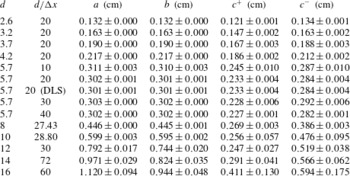
Figure 2 provides information on the shapes of the droplets. The implication of the results depicted there is twofold. First, note that for droplets with
 $d<10~\text{mm}$
, the equatorial semi-axes
 $a,b$
of the bi-ellipsoid essentially coincide, while the sagittal semi-axes
 $c^{\pm }$
deviate with increasing droplet diameter. This indicates that the deformation occurs essentially orthogonal to the centre axis, without any preferred direction. For larger droplets, however, the asymmetry within the equatorial plane becomes more pronounced, i.e. the droplets are stretched in a direction orthogonal to the centre axis. Interestingly, the deviation of the sagittal semi-axes
 $c^{\pm }$
decreases for droplets with
 $d>12~\text{mm}$
, which indicates the decreasing performance of the bi-ellipsoid model in terms of shape representation, cf. table 8. Figure 2 compares the shape estimation errors of the bi-ellipsoid representation and spherical harmonics decomposition. While the error of the bi-ellipsoid representation and the spherical harmonics decomposition with
 $L=1$
are in the same order of magnitude for the 2.6 mm droplet, increasing droplet size is accompanied by a considerable deviation. Due to the weak deformation, the error of the bi-ellipsoid fitting retains its magnitude of
 $1\times 10^{-6}$
for droplets up to 4.2 mm, lying roughly two orders of magnitude below the spherical harmonics decomposition with an identical number of parameters. Within the range of 4.2 and 10 mm, the error of the bi-ellipsoid fitting increases by two orders of magnitude, resembling the
 $L=4$
curve. Thus, the applicability of the bi-ellipsoid fitting is restricted to droplets with
 $d<10~\text{mm}$
. Note that the curves for
 $L=4$
and
 $L=8$
show increasing deviation for droplets with
 $d>4.2~\text{mm}$
, which indicates the broadening complexity of surface deformation.
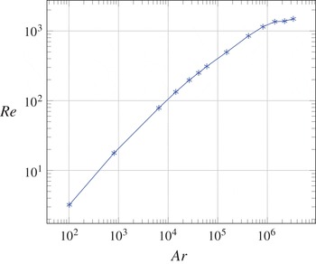
Just as the drag curve shows non-monotone behaviour, the same is true for the terminal velocity as a function of the droplet diameter; cf. table 5 and see figure 37 below. This complexity is partly related to the velocity being an output parameter, which is strongly influenced by the differing qualitative rise behaviour, rather than a pre-fixed input to the experiment. This has already been mentioned in § 2.3, where the Archimedes number was introduced as an appropriate dimensionless volume which – in a log–log-plot – can be used as a shifted dimensionless diameter. It is, hence, interesting to study the output parameter
 $\mathit{Re}$
as a function of the input parameter
 $\mathit{Ar}$
. The relationship obtained for the simulated droplets is displayed in figure 5, showing a strictly monotonic increase of
 $\mathit{Re}$
with
 $\mathit{Ar}$
. In fact the relation is almost linear up to
 $\mathit{Ar}\approx 10^{6}$
, followed by a range with much smaller slope.
Reynolds number as a function of Archimedes number, demonstrating a monotonic increase in Reynolds number that plateaus for the largest droplets.

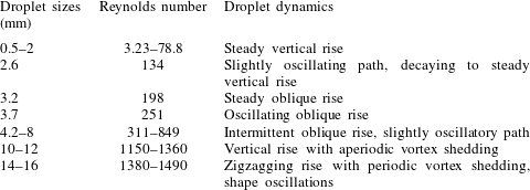
The sharp increase in the drag coefficient, as well as the trend towards a plateau in the Reynolds number as a function of the Archimedes number, is related to severe changes in the qualitative rise behaviour in terms of particle path, wake and shape. A detailed study of the underlying droplet dynamics is deferred to the next section, while the prototypical behaviour of the droplets is summarized in table 6. The qualitative picture is as follows:
Prototypical rise dynamics for droplets of different sizes.

Droplets in our study of size smaller than 2.6 mm rise on a vertical path. Their flow field may exhibit a varying number of vortices inside the droplet and in the wake. The flow fields of these droplets are axisymmetric.
For larger droplets, the route to chaotic behaviour seems analogous to the bifurcation behaviour found by numerical stability analysis for fixed spheres and ellipsoids with no-slip (Natarajan & Acrivos Reference Natarajan and Acrivos1993) and free-slip boundary conditions (Yang & Prosperetti Reference Yang and Prosperetti2007; Tchoufag et al. Reference Tchoufag, Magnaudet and Fabre2013).
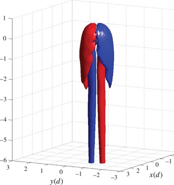
A first bifurcation occurs in the diameter range from 2.6 to 3.2 mm, since the 3.2 mm droplet is the first one to clearly rise on a path not aligned with gravity. Instead, this droplet shows a steady sidewards migration, accompanied by sheets of streamwise vorticity. These sheets of streamwise vorticity are symmetric about the plane of the droplet centre path; axisymmetry, however, is lost. This corresponds to the first, regular bifurcation reported in the above mentioned works.
Another qualitative change in rise behaviour is observed for the 3.7 mm droplet. The terminal state in this simulation is not stationary anymore. Instead, the wake of the droplet becomes wavy, and the droplet rises on an oscillatory path. This can be attributed to a Hopf bifurcation analogous to the ones found numerically in Yang & Prosperetti (Reference Yang and Prosperetti2007) and Tchoufag et al. (Reference Tchoufag, Magnaudet and Fabre2013).
The droplets of sizes 4.2–8 mm show a more irregular behaviour. Smaller droplets in this range rise in a manner similar to the 3.2 mm droplet. They rise on a piecewise straight path. However, the plane in which this movement takes place is not constant in time but changes its orientation abruptly in a non-periodic manner. The frequency of orientation changes increases with increasing droplet diameter.
For larger droplets of sizes 10 and 12 mm, the rise path is smooth and almost vertical. The 12 mm droplet, however, seems to be in a transitional regime already, where the vertical rise is interrupted by short periods of oscillating behaviour. Both droplets exhibit aperiodic vortex shedding without a clear connection between shedding and their rise path.
Finally, the largest droplets of sizes 14 and 16 mm rise on zigzag-paths. The plane in which the zigzagging takes place, however, is not constant in time but is subject to irregular rotations. Their rise path is intimately coupled to a periodic shedding of vortices.
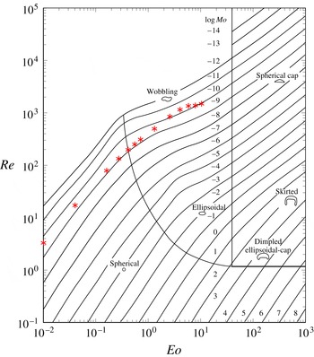
In figure 6, the simulation results of our study are classified in the Grace Diagram (Clift et al.
Reference Clift, Grace and Weber2005), where prototypical behaviour of rising bubbles and droplets in dependence on Re,
 $\mathit{Eo}$
and
 $\mathit{Mo}$
is summarized. Considering that the Morton number in this work is
 $\mathit{Mo}=1.00\times 10^{-10}$
, the agreement is satisfactory. The droplets of sizes 0.5–2.6 mm lie well beneath the boundary of the ‘spherical’ regime, in agreement with our results. As suggested by the Grace diagram, droplets larger than 3.2 mm do not show an ellipsoidal form on a straight rising path. Instead, they undergo intricate paths, and the largest ones show rocking movements on oscillatory paths.
Simulations in this work, plotted into the Grace diagram taken from Clift et al. (Reference Clift, Grace and Weber2005).

5. Results on droplet dynamics
Depending on the droplet size, the dynamic behaviour can change drastically. However, we identify different regimes of motion, group them according to their prototypical behaviour and describe the pertinent flow features in the following section.
5.1. Steady, vertical rise
5.1.1. Rise path
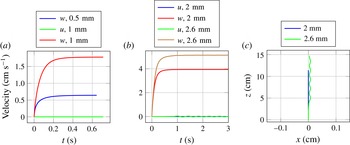
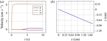
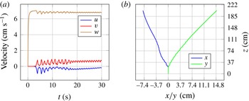
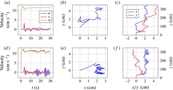
The smallest droplets considered here, with sizes of 0.5, 1 and 2 mm exhibit a steady vertical rise; cf. figure 7. After the start of the simulation, buoyancy accelerates the droplets monotonically until the terminal velocity is reached. There are no significant lateral velocities observed, and the asymptotic state is stationary, which means there are neither oscillations of droplet shape nor oscillations of the path velocity. Due to the high curvature and the small terminal rise velocity, surface tension forces are so strong compared to hydrodynamic forces that no significant deviation of the droplet from the spherical shape can be observed. The Weber numbers in this regime are much smaller than one, consistent with the dominance of surface tension effects over droplet inertia in this region; cf. table 5.
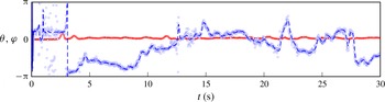
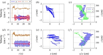
Velocity of the centre of mass of the 0.5, 1, 2 and 2.6 mm droplet are shown in the left two figures, where
 $w$
is the vertical or
 $z$
-component and
 $u$
is the lateral or
 $x$
-component. In the right figure, the motion in the
 $xz$
-plane is shown. Only the 2.6 mm displays a lateral motion.

Similar observations hold for the terminal behaviour of the 2.6 mm droplet. However, this droplet is in a transitional regime. Before reaching terminal velocity, the lateral velocity component starts to oscillate slightly, leading to an oscillation of the rise path. This oscillation, however, is damped in time, and the terminal state seems to be a steady vertical rise, or a path with oscillations of very small amplitude.
In general, the time needed to approach terminal velocity increases with droplet size; cf. again figure 7.
5.1.2. Velocity field
For very small droplets,
 $\mathit{Re}$
is much less than one and the shape is nearly spherical, in which case the associated velocity field can be approximated using analytical solutions. The solution for creeping flow (
 $\mathit{Re}=0$
) was derived by Hadamard (Reference Hadamard1911) and Rybczynski (Reference Rybczynski1911). The stream function of the solution is axisymmetric and symmetric with respect to the equatorial plane of the droplet (fore-aft symmetry). For very small Reynolds numbers, the VOF-code FS3D can reproduce the Hadamard–Rybczynski velocity field (Weirich et al.
Reference Weirich, Köhne and Bothe2014). Moreover, the Hadamard–Rybczynski solution also yields an analytical prediction of the terminal rise velocity, which shows good agreement with experimental results for sufficiently small gas bubbles in ultra-clean water (Parkinson et al.
Reference Parkinson, Sedev, Fornasiero and Ralston2008).
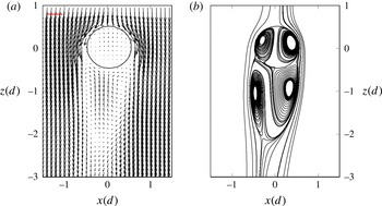
The 0.5 mm droplet exhibits a Reynolds number of
 $\mathit{Re}=3.23$
, with
 $\mathit{Re}$
based on the droplet diameter. The velocity field is axisymmetric, but does not show the fore-aft symmetry predicted by the Hadamard–Rybczynski solution, which therefore does not provide a qualitatively correct approximation at this Reynolds number. In fact, the Hadamard-Rybczinski solution predicts a terminal velocity of
 $1.14~\text{cm}~\text{s}^{-1}$
as opposed to a simulated rise velocity of
 $0.65~\text{cm}~\text{s}^{-1}$
.
A weakly nonlinear extension to small, non-vanishing, Reynolds numbers of the creeping flow solution was given in Taylor & Acrivos (Reference Taylor and Acrivos1964) using a method of matched asymptotics that was motivated by the earlier singular perturbation work of Proudman & Pearson (Reference Proudman and Pearson1957) for flow past a solid sphere. Taylor and Acrivos’s singular perturbation assumes axisymmetric flow and includes small deviations from a spherical geometry. Taylor & Acrivos (Reference Taylor and Acrivos1964) provide the analytical drag correlation
 $$\begin{eqnarray}\displaystyle C_{D} & = & \displaystyle \frac{8}{\mathit{Re}}\left(\frac{3\tilde{{\it\mu}}+2}{\tilde{{\it\mu}}+1}+\left(\frac{3\tilde{{\it\mu}}+2}{\tilde{{\it\mu}}+1}\right)^{2}\frac{\mathit{Re}}{16}\right.\nonumber\\ \displaystyle & & \displaystyle \left.+\,\left(\frac{3\tilde{{\it\mu}}+2}{\tilde{{\it\mu}}+1}\right)^{3}\frac{\mathit{Re}^{2}}{160}\log _{10}\frac{\mathit{Re}}{2}+\frac{{\it\mu}_{c}^{2}{\it\lambda}\left(3\tilde{{\it\mu}}^{2}-\tilde{{\it\mu}}+8\right)}{10(\tilde{{\it\mu}}+1)^{2}{\it\sigma}{\it\rho}d}\mathit{Re}^{2}\right)\end{eqnarray}$$
with
 $\mathit{Re}=({\it\rho}_{c}\,\text{d}U_{t})/{\it\mu}_{c}$
and
 $$\begin{eqnarray}{\it\lambda}=\frac{1}{4(\tilde{{\it\mu}}+1)^{3}}\left(\frac{81}{80}\tilde{{\it\mu}}^{3}+\frac{57}{20}\tilde{{\it\mu}}^{2}+\frac{103}{40}\tilde{{\it\mu}}+\frac{3}{4}-\frac{\tilde{{\it\rho}}-1}{12}(\tilde{{\it\mu}}+1)\right).\end{eqnarray}$$
The respective terminal velocities can then be obtained by equating the drag and lift forces, i.e. finding the roots of
 $$\begin{eqnarray}f(U_{t})=g{\rm\Delta}{\it\rho}\frac{4d}{3}-{\it\rho}_{c}U_{t}^{2}C_{D}\left(\frac{U_{t}{\it\rho}_{c}d}{{\it\mu}_{c}}\right).\end{eqnarray}$$
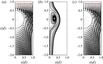
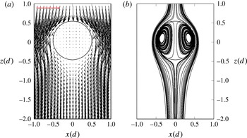
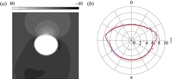
For comparison, on the right panel of figure 8, the velocity field according to Taylor–Acrivos is shown. All velocity plots show the velocity in the frame co-moving with the full droplet centre of mass velocity.
Velocity field around the 0.5 mm droplet (
 $\mathit{Re}=3.23$
). The horizontal arrow at the upper edge indicates the length of a velocity vector of modulus
 $U_{t}$
. For comparison, the figure on the right-hand side shows the analytic solution obtained by Taylor & Acrivos (Reference Taylor and Acrivos1964).

The predicted terminal velocity is
 $0.66~\text{cm}~\text{s}^{-1}$
with the theory from Taylor & Acrivos (Reference Taylor and Acrivos1964), very close to the simulated value of
 $0.65~\text{cm}~\text{s}^{-1}$
. The agreement of the velocity fields is still reasonable, although the Reynolds number is already too high to consider the Taylor–Acrivos solution strictly applicable, and the numerical solution suffers from parasitic currents caused by the high interface curvature. Note that the Reynolds number employed in Taylor & Acrivos (Reference Taylor and Acrivos1964) is based on the radius of the droplet, hence half of the value given here.
Inside the droplet, the velocities are less than 1 % of the rise velocity; see figure 8 and note the horizontal arrow at the top which depicts the rise velocity. The trajectories of virtual tracer particles show that a ring vortex, similar to Hill’s spherical vortex, is formed.
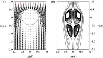
The flow field of the 1 mm droplet is qualitatively similar to the one of the 0.5 mm droplet, see figure 9. However, due to the much higher Reynolds number (
 $\mathit{Re}=17.78$
), the asymmetry about the equatorial plane is more pronounced, and the ring vortex inside the droplet is stronger.
Velocity field around 1 mm droplet. The horizontal arrow at the upper edge indicates the length of a velocity vector of modulus
 $U_{t}$
.

The velocity field in and around the 2 mm droplet is shown in figure 10. It is observed that the Hill vortex inside the droplet is again stronger than that in the 1 mm droplet. This is in accordance with the findings in Oliver & Chung (Reference Oliver and Chung1987), who noted that the strength of the internal circulation increases with
 $\mathit{Re}$
.
Velocity field around 2 mm droplet. The horizontal arrow at the upper edge indicates the length of a velocity vector of modulus
 $U_{t}$
.

The most salient new flow structure visible for the 2 mm droplet is the onset of a closed recirculating region in the wake. The onset of a downstream standing eddy is well understood in the case of rigid spherical particles in a uniform flow. A consensus exists that the critical Reynolds number for the onset of a standing eddy is 20 (Clift et al. Reference Clift, Grace and Weber2005, p. 102), explained by flow separation of the viscous boundary layer around the sphere.
In the case of deformable fluid particles the situation is more complicated, and the occurrence of vortices beneath the droplet depends to a large extent on the viscosity ratio
 $\tilde{{\it\mu}}$
and aspect ratio
 ${\it\alpha}$
. In the wake of spherical fluid particles (
 ${\it\alpha}=1$
) whose viscosity is smaller or equal to that of the surrounding fluid (
 $\tilde{{\it\mu}}\leqslant 1$
), no vortices are found in the wake. This was experimentally noted in Winnikow & Chao (Reference Winnikow and Chao1966) and numerically in Rivkind & Ryskin (Reference Rivkind and Ryskin1976). Dandy & Leal (Reference Dandy and Leal1986) performed simulations for ellipsoidal particles with a fixed shape in the case of a vanishing disperse phase viscosity. They found that for sufficiently large deviations from the spherical case, standing eddies can occur for intermediate Reynolds numbers. For small or very large
 $\mathit{Re}$
they are not observed. They show that two conditions must be fulfilled for the existence of standing eddies: the rate of vorticity production at the free surface must be sufficiently large, and the rate of downstream transport of vorticity must be sufficiently small. These findings were qualitatively confirmed by Blanco & Magnaudet (Reference Blanco and Magnaudet1995). In that work, vortices are only found for
 ${\it\chi}>1.65$
, where
 ${\it\chi}:=1/{\it\alpha}$
is the inverse aspect ratio.
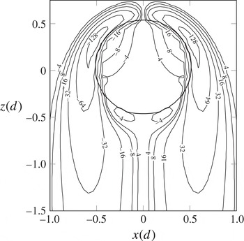
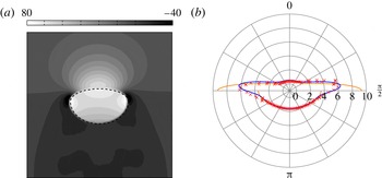
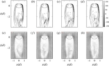
As can be seen in figure 10, the vortices inside and outside the droplet have the same sense of rotation. For reasons of flow topology, one would expect that a counter rotating vortex should be found near the rear end of the droplet. In our simulations however, such a vortex does not occur, although vorticity changes sign in a small region close to the rear end of the droplet, as visible in figure 11.
Vorticity isolines around 2 mm droplet. Vorticity in
 $\text{s}^{-1}$
.

The explanation for this is that the vortices in the droplet wake are not caused by flow separation at the free interface. As mentioned above, those vortices are a phenomenon of intermediate Reynolds numbers and cannot be explained by boundary layer theory, which predicts that no separation occurs on fluid interfaces. Instead, as was discussed in the literature (Rivkind & Ryskin Reference Rivkind and Ryskin1976; Dandy & Leal Reference Dandy and Leal1986; Blanco & Magnaudet Reference Blanco and Magnaudet1995), the standing eddies are a result of vorticity accumulating downstream of the droplet and inducing the formation of a vortex.
Therefore, the vortex in the wake and the interface are spatially separated from each other, allowing for a flow structure as shown in figure 10. This is in accordance with the experimental results in Sumner & Moore (Reference Sumner and Moore1969) and LeClair et al. (Reference LeClair, Hamielec, Pruppacher and Hall1972). We would like to point out, however, that Pruppacher & Beard (Reference Pruppacher and Beard1970) have experimentally found counter rotating vortices in water drops falling in air. Rivkind & Ryskin (Reference Rivkind and Ryskin1976) have found the same vortex structure in their simulations for very high viscosity ratios of
 $\tilde{{\it\mu}}=100$
.
The velocity field of the 2.6 mm droplet is very close to the one observed on the 2 mm droplet. The path instability is hardly recognizable in the streamlines.
5.1.3. Comparison between analytical solutions and numerical results
The droplets considered in this work have a Reynolds number that is too high to be strictly approachable by analytical solutions based on Stokes flow or perturbations thereof. Nevertheless, it is valuable to compare the numerical solution with analytical results for the smallest diameter of 0.5 mm, aiming for a mutual validation.
One should first note that at this Re, the shape of the 0.5 mm droplet is very close to spherical and due to the large oil viscosity, the droplet’s surface is almost immobile. Therefore, several analytical correlations, as collected in figure 3(b), are of interest. The resulting predictions for the terminal velocity are
 $0.703~\text{cm}~\text{s}^{-1}$
from Goldstein (Reference Goldstein1929),
 $0.688~\text{cm}~\text{s}^{-1}$
from Proudman & Pearson (Reference Proudman and Pearson1957) and
 $0.655~\text{cm}~\text{s}^{-1}$
from Taylor & Acrivos (Reference Taylor and Acrivos1964). Such close values from different solutions with different approximation orders indicate that the solutions are in the vicinity of the true rise velocity. Moreover, these values agree well with the simulated rise velocity of
 $0.646~\text{cm}~\text{s}^{-1}$
.
Most importantly, the agreement between the simulation and the solution of Taylor & Acrivos (Reference Taylor and Acrivos1964) with a deviation of the terminal velocity of less than 2 % is by far the best. This is to be expected from the physics. It strongly indicates the high quality of the DNS result.
Let us note in passing that Moremedi & Mason (Reference Moremedi and Mason2010) applied analytical solutions to rising drops at quite high Reynolds numbers and found some of the pertinent flow features predicted by the low Reynolds number solutions.
In order to compare the full velocity fields for the 0.5 mm droplet to the analytical solutions of Taylor & Acrivos (Reference Taylor and Acrivos1964), we define a global relative error via
 $$\begin{eqnarray}\mathscr{E}:=\frac{\displaystyle \int _{{\it\Omega}}|\boldsymbol{v}-\boldsymbol{v}_{TA}|\,\text{d}x\,\text{d}z}{|{\it\Omega}|\,|U_{t}|},\end{eqnarray}$$
where
 $\boldsymbol{v}_{TA}$
is the solution of Taylor–Acrivos, and
 ${\it\Omega}=[-1d,1d]\times 0\times [-2d,1d]$
. Due to the axisymmetry of the solutions, this is the same as integrating over the associated rotational cylinder. Note that for the normalization in (5.4), the terminal velocities
 $U_{t}$
from the DNS are used. The computations were performed both with the actual rise velocity from the simulations and with the analytical prediction according to Taylor–Acrivos. We found that the Taylor–Acrivos velocity field shows a reasonable agreement, with a global error of less than 8 %. The main contributions to the global error stem from the upstream region, while the internal circulation and the downstream region contribute one to two orders of magnitude less. If the velocity field from Taylor & Acrivos (Reference Taylor and Acrivos1964) is rescaled using the terminal velocity from the DNS, the global error is below 7 %.
5.2. Steady, oblique rise
5.2.1. Path
As opposed to smaller droplets, the 3.2 mm droplet does not rise on a vertical path, see figure 12. Instead, it rises in a straight path skewed to gravity at an angle of
 $3.16^{\circ }$
. After the initial transition, the terminal state is quasi-stationary, without oscillations of any kind. Similar behaviour, i.e. lateral migration with a stationary terminal state, was noticed in the simulations of rigid spheres in Jenny et al. (Reference Jenny, Dusek and Bouchet2004).
Centre of mass velocity and projection of rising path onto
 $xy$
-plane of 3.2 mm droplet.

For the 3.2 mm droplet, the streamwise (
 $z$
-) component of vorticity is non-negligibly large, cf. figure 13, where isosurfaces of streamwise vorticity are shown. This structure is referred to as a bifid wake. This is not the case for the smaller droplets, where the streamwise vorticity is at least one order of magnitude smaller in the numerical computations and does not exhibit a bifid wake. In experiments where the flow is visualized by dye, a bifid wake can be seen as two threads trailing behind the droplet (Winnikow & Chao Reference Winnikow and Chao1966; Sanada, Shirota & Watanabe Reference Sanada, Shirota and Watanabe2007). The flow changes from axisymmetric to a flow with a single symmetry plane.
Bifid wake:
 $1~\text{s}^{-1}$
(red) and
 $-1~\text{s}^{-1}$
(blue) isosurfaces of streamwise vorticity.

The same wake structure is found for flow around a fixed rigid sphere; the critical Reynolds number in this case is about 212, cf. Natarajan & Acrivos (Reference Natarajan and Acrivos1993) and Tezuka & Suzuki (Reference Tezuka and Suzuki2006). This vorticity introduces a lift force on the bubble (De Vries, Biesheuvel & Van Wijngaarden Reference De Vries, Biesheuvel and Van Wijngaarden2002), which can explain the fact that the droplet path becomes oblique. Therefore, it is reasonable to conclude that the wake instability induces the path instability.
Yang & Prosperetti (Reference Yang and Prosperetti2007) performed a linear stability analysis of flow around spheroids with a fixed-shape and a free-slip boundary condition. After variation in
 ${\it\chi}$
, they found that this bifid wake corresponds to the first bifurcation taking place after a variation in
 ${\it\chi}$
. The bifurcation is regular, corresponding to time-independent behaviour.
The velocity field in the wake is similar to that of the 2 mm droplet, although the vortex is skewed in accordance with the oblique rise direction, see figure 14. Similar flow fields can be found for flow around fixed spheres, see Johnson & Patel (Reference Johnson and Patel1999, figure 11).
Flow field of 3.2 mm droplet, relative to full terminal velocity.

Also note that for rigid particles on oblique paths, a slow rotation around an axis perpendicular to the rise plane is observed as mentioned e.g. in Jenny et al. (Reference Jenny, Dusek and Bouchet2004). For fluid particles, the broken axisymmetry does not lead to a rotation of the fluid particle as a whole, but to a deformation of the inner flow field such that viscous forces can counter-balance the torque resulting from the lift force.
5.3. Oscillatory, oblique rise with wavy wake
Similar to the 3.2 mm case, the 3.7 mm droplet rises approximately in a plane skewed to the direction of gravity. The main difference is that the asymptotic behaviour is not time independent; instead, the rise velocity shows a small oscillation around the straight path, see figure 15. The path is slightly stronger inclined, with a mean angle of
 $5.96^{\circ }$
. Again, this bifurcation behaviour is analogous to that observed for the rise of rigid particles, cf. Jenny et al. (Reference Jenny, Dusek and Bouchet2004).
Centre of mass velocity and projection of path onto
 $xz$
- and
 $yz$
-plane for the 3.7 mm droplet.

Normalized single-sided amplitude spectra of velocities for the 3.7 mm droplet.

Periodic vortex shedding, 3.7 mm droplet. In the left panel, the
 $-0.25$
Pa isosurface of pressure is shown. In the middle, the velocity field in the gray plane is depicted, together with the
 $-0.25$
Pa isolines of pressure. Data are shown at times 27.9125, 28.0125, 28.1125, 28.2125 and 28.3125 s. On the right-hand side, the
 $\pm 2.5~\text{s}^{-1}$
isosurfaces of streamwise vorticity are shown. The vortex shedding frequency is about 2.1 Hz.

The rise velocity does not increase monotonously with time anymore. Instead, after the initial release, the
 $z$
-component of the velocity increases with vanishing lateral velocities until path instability sets in. At this point, the lateral velocities experience a rapid increase, while the rise velocity decreases sharply. After that, periodic oscillations set in. The amplitude of the oscillations are initially quite strong, but they are damped in time until they approach an asymptotic value. In the oscillating regime, the lateral centre of mass velocity of the droplet increases until a local maximum is reached. This coincides with a maximum of the inclination angle and a minimum of rise velocity. The droplet then recoils. At the moment of maximal lateral velocities, the droplet is most oblate. The frequency of this mechanism is 1.05 Hz, corresponding to a Strouhal number of 0.0574.
Jenny et al. (Reference Jenny, Dusek and Bouchet2004) find a difference in the bifurcation behaviour for fixed spheres, depending on their density ratio
 $\tilde{{\it\rho}}$
. For
 $\tilde{{\it\rho}}<2.5$
, they find that the secondary Hopf bifurcation is not that of a fixed sphere. Instead, they find oscillations with a Strouhal number of 0.051, which is much smaller than the value found for fixed spheres of about 0.127. Since the density of the oil droplets here is below the threshold, our results are in accordance with their findings.
In figure 16, the normalized single-sided amplitude spectra (
 $P$
) of the discrete Fourier transforms of the velocity components are shown. All velocities show clear peaks at 1.05 Hz. The 2.1 Hz peak coincides with the frequency of vortex shedding, which takes place with twice the frequency of the velocity oscillation. The vortex shedding frequency is determined by examining the periodicity of the pressure and velocity fields, cf. figure 17. In fact, a vortex is shed at the minimal and maximal values of the lateral velocities. In figure 17, in the leftmost pane, the
 $-0.25$
Pa isosurface of pressure is depicted. The first row of figures corresponds to a minimum of lateral velocities, whereas the last row corresponds to a time where the lateral velocities are maximal. It is observed that a region of low pressure is shed beneath the droplet in a time periodic manner. This low pressure region has the shape of an incomplete horseshoe vortex. In the middle pane, we see the velocity components orthogonal to streamwise direction in a plane 3.975 droplet diameters beneath the droplet centre, as well as the intersection of the
 $-0.25$
Pa pressure isosurface with the plane. It can be clearly seen that the low pressure region indicates a vortex. Considering the streamwise velocity component in the wake, we no longer find a bifid wake; see the rightmost pane of figure 17. Instead, vorticity threads of alternating sign are observed.
5.4. Intermittent oblique rise
The droplets from 4.2 to 8 mm do not rise in a single plane anymore. Instead, they rise on paths which are piecewise straight, but change in direction regularly, see figure 18.
Centre of mass velocity (a–c), rising path in
 $xy$
-plane (d–f) and rising path in
 $xz/yz$
-plane (g–i) of 4.2, 5.7 and 8 mm droplet (left to right).

The sharp drop in rise velocity, accompanied by the sudden increase in lateral velocities, after the initially rectilinear rise becomes more pronounced with a higher droplet diameter. The frequency of the direction changes increases with droplet diameter. However, the dimensionless maximal deviation of the droplet centre of mass from its initial position decreases with diameter: while the 5.7 mm droplet travels approximately
 $20d$
laterally from the initial position, the 8 mm droplet’s maximal lateral deviation is little more than
 $5d$
.
For rising air bubbles, spiral or zigzagging paths are often reported (Ellingsen & Risso Reference Ellingsen and Risso2001; Mougin & Magnaudet Reference Mougin and Magnaudet2001). It is typically reported that bubbles change from a zigzagging path into a spiral one. In the present simulations, we do not find paths of that kind. As was noted in the previous two sections, the rising behaviour of high viscosity oil droplets is closely related to that of fixed spheres. The question of whether freely rising rigid spheres show oscillatory behaviour was experimentally studied in Horowitz & Williamson (Reference Horowitz and Williamson2010). There, it was found that a critical density ratio
 $\tilde{{\it\rho}}$
exists, above which no zigzagging occurs. For
 $\mathit{Re}<1550$
, this critical ratio was found to be 0.4. Spheres above this ratio showed intermittent oblique behaviour. As
 $\tilde{{\it\rho}}$
is well above this threshold in our simulations, our results are in accordance with these findings.
The streamwise component of vorticity for the 4.2 mm droplet is similar to the 3.7 mm case. However, for the smaller droplet we found one symmetry plane, while for the 4.2 mm droplet, the symmetry plane becomes unstable and changes with time. In figure 19, such a change in rise direction is depicted. We see that, at the moment of minimal lateral velocities, the streamwise vorticity is negligible, and the sheets of streamwise vorticity surrounding the droplet change their orientation to account for the new rise direction; cf. the discussion in § 5.2.
Streamwise vorticity of 4.2 mm droplet before, during and after the change of sign of the
 $u$
-velocity component.
 $\pm 5~\text{s}^{-1}$
isosurfaces of streamwise vorticity is shown at times 17.5, 18.5 and 19.5 s.

While the shape of the 4.2 mm droplet is close to an ellipsoidal shape, the droplets of size 5.7 and 8 mm appear to be composed of an upper part and a lower part, both of which are halves of ellipsoids with different aspect ratios. The bi-ellipsoidal shape can be explained by examination of the local pressure distribution near the droplet surface, cf. figure 23(a). At the north pole of the droplet, the dynamic pressure is higher due to inertial forces. This leads to an overall fore–aft pressure jump to which the droplet reacts by shape adaptation due to
 $\mathit{We}>1$
. The pressure field inside the droplet is rather homogeneous since the inner circulation is strongly damped because of the high droplet viscosity. Note also that the hydrostatic pressure only gives a minor contribution (
 ${<}10~\text{Pa}$
) to the internal variation. The overall pressure variation inside the droplet is about 20 Pa for the 5.7 mm droplet. The pressure level ranges from 120 to 140 Pa, where the smallest value occurs at the poles, the largest values can be found at the equatorial plane and the droplet exhibits a pressure saddle point of about 130 Pa, cf. figure 20.
Close-up of pressure field (in Pa) inside the 5.7 mm droplet with isolines (red) and interface (dashed).

With a convex shape and negligible pressure jump contribution due to viscous stress, the pressure is higher inside the droplet, in agreement with the Young–Laplace law. Consequently, the pressure jump is significantly smaller at the north pole compared to the south pole, resulting in two different curvature levels, cf. figure 23(b). Hence, a bi-ellipsoidal shape is formed. The transition between the two half ellipsoids at the droplet’s equator is rather sharp because the Bernoulli effect induces an additional pressure jump there.
For a closer examination of the droplet shape see the next section.
5.4.1. Shape analysis (only
 $5.7~\text{mm}$
)

This section provides information on the shape of the 5.7 mm droplet using the tools introduced in 3.4. As can be seen from figure 21, the first principal axis
 $\boldsymbol{t}_{3}$
of the droplet shows good agreement with the rise velocity vector after the initial acceleration phase, i.e. for
 $t\geqslant 3~\text{s}$
. There is no significant phase shift, which suggests that path and shape changes occur essentially simultaneously. Further, the evolution of the azimuthal and polar angles indicate a nearly vertical rise direction, accompanied by back and forth polar rotations. Note that the agreement for the azimuthal angle (RMS:
 $6.50\times 10^{-5}$
) is better than for the polar angle (RMS:
 $-4.54\times 10^{-4}$
). The droplet deforms to a bi-ellipsoidal shape during the acceleration phase and retains its shape while undergoing rocking movement, cf. figure 22.
Azimuthal (
 ${\it\theta}$
) and polar (
 ${\it\varphi}$
) angle of principal axis
 $\boldsymbol{t}_{3}$
(
 ${\it\theta}$
: ○,
 ${\it\varphi}$
: ▫) and droplet centre velocity (
 ${\it\theta}$
: solid,
 ${\it\varphi}$
: dashed) for 5.7 mm droplet (
 $d/({\rm\Delta}x)=20$
).

 $xz$
-sections for 5.7 mm droplet (left:
 $t=0~\text{s}$
,
 ${\rm\Delta}t=5~\text{s}$
) with normalized centre velocity (red).

Because the curvature incorporates second spatial derivatives of the level set function, which is discontinuous at the equatorial plane, the numerical results cannot be rendered correctly in its vicinity, i.e. for
 ${\it\theta}\approx {\rm\pi}/2$
, at least for the direct computation, cf. § 3.4.2. As figure 23 clearly indicates, both methods show good agreement in the vicinity of the poles. However, the smoothed transition provides a reliable approximation also at the equatorial plane. Despite the strong deformation due to decreasing surface tension forces, the curvature can globally be well approximated by the smoothed bi-ellipsoid shape, demonstrating the applicability of this model. As table 7 and figure 2 exhibit, this trend is sustained for increasing droplet size. As can be seen from table 7, the residual of the shape representation using the four parameter bi-ellipsoid is only one order of magnitude below the spherical harmonics decomposition with 81 coefficients. However, the bi-ellipsoid is well suited for this regime.
(a) Pressure in Pa in
 $xz$
-plane for 5.7 mm droplet (
 $[-(3d)/2,(3d)/2]^{2}$
, DLS) at
 $t=33~\text{s}$
with bi-ellipsoid interface fit (dashed), cf. figure 20 for a close-up; (b) associated numerical curvature (
 $\times$
) versus curvature of bi-ellipsoid (orange: direct computation, blue: smoothed with
 $k=10$
; cf. (3.4)) in
 $\text{cm}^{-1}$
over azimuthal angle
 ${\it\theta}\in [0,{\rm\pi}]$
.

For the 5.7 mm droplet, the absolute values of the residuals are of magnitude
 $10^{-5}$
, indicating a very good agreement between analytical and effective shape. In figure 23, the pressure and curvature are examined for a
 $xz$
section at the droplet centre of mass. The curvature is compared to the analytical values, computed both directly and with smoothed transition.
LSE residuals for surface reconstruction: bi-ellipsoid fitting with 4 parameters versus spherical harmonics fitting of degree
 $L$
with
 $(L+1)^{2}$
parameters, cf. figure 2.

Mean values and standard deviations of bi-ellipsoid semi-axes.

5.5. Vertical rise with aperiodic vortex shedding
In figure 24, silhouettes of the droplets from 10 to 16 mm are shown. The silhouettes are computed by intersecting the droplet interface with a fixed plane that cuts the droplet centre of mass. Every droplet was tracked over a time span of 3 s, and the time difference between two adjacent silhouettes is 0.2 s.
Intersection of the droplet surface (reconstructed from spherical harmonics; for the 14 and 16 mm droplet ellipsoid compression was applied, cf. § 3.4) with
 $xz$
-plane over a time period of 3 s for 10, 12, 14 and 16 mm droplet (left to right). Time between two frames is 0.2 s. The scale on the
 $x$
-axis also applies to the axis of ordinates.

Centre of mass velocity and projection of path onto
 $xz$
- and
 $yz$
-plane of 10 and 12 mm droplet.

We see that the 10 and 12 mm droplets rise almost vertically without any significant time dependence of the shape, cf. figure 25. Their shape appears bi-ellipsoidal, similar to the shapes of the 5.7 and 8 mm droplets.
Shape analysis
The bi-ellipsoidal shape, cf. figure 26, can be explained by an argumentation analogous to the one given above for the 5.7 mm droplet.
(a) Pressure in Pa in
 $xz$
-plane for 10 mm droplet (
 $[-3d/2,3d/2]^{2}$
) at
 $t=39~\text{s}$
with bi-ellipsoid interface fit (dashed); (b) associated numerical curvature (
 $\times$
) versus curvature of bi-ellipsoid (orange: direct computation, blue: smoothed with
 $k=6$
; cf. (3.4)) in
 $\text{cm}^{-1}$
over azimuthal angle
 ${\it\theta}\in [0,{\rm\pi}]$
.

There are no large scale shape oscillations present. Vortices are shed in an aperiodic manner, and there is no obvious connection to the changes in rising path.
The wake of the 10 mm droplet is no longer cone-like. Instead, it resembles a circular cylinder with diameter 10 mm, see figure 27. The wake is bounded by an almost cylindrical sheet of high vorticity. At the lower end, vortices form and are shed in the downstream direction. However, directly behind the droplet there is a zone of low relative velocities, and the vortices are also sucked in the upstream direction towards the centre of the droplet.
Wake of 10 mm droplet: (a,e)
 $=13.35$
s; (b,f)
 $=13.50$
s; (c,g)
 $=13.65$
s; (d,h)
 $=13.80$
s. In (a–d), isolines of
 $yz$
-vorticity are shown. In (e–h), the velocity field in the wake is depicted.

Regarding the shape description in terms of bi-ellipsoids, the implications of the residuals given in table 7 are twofold. First, the absolute value of the residual for the 10 mm droplet is of magnitude
 $10^{-4}$
, indicating a good agreement between analytical and effective shape. Figure 26 compares the numerical curvature to the curvature of the fitted bi-ellipsoid, computed both directly and with smoothed transition. Again, both methods show good agreement in the vicinity of the poles. However, the smoothed transition provides a reliable approximation also at the equatorial plane. Despite the strong deformation due to decreasing surface tension forces, the curvature can globally be well approximated by the smoothed bi-ellipsoidal shape, demonstrating the applicability of this model. In comparison to the 5.7 mm droplet, the residual has increased by one order of magnitude, indicating a decrease in performance of the bi-ellipsoid model. As table 7 clearly shows, this trend continues for increasing droplet size.
5.6. Zigzagging rise with periodic vortex shedding
The 14 and 16 mm droplets show a zigzagging path, where the plane in which the zigzag movement takes place is not constant in time but is subject to spurious rotations, see figures 28.
Centre of mass velocity and projection of path onto
 $xz$
- and
 $yz$
-plane of 14 mm (a–c) and 16 mm (d–f) droplet.

The droplet shape is still approximately bi-ellipsoidal, but the order of magnitude of the shape error has increased by one order of magnitude compared to the 10 mm droplet. From a view perpendicular to the plane in which the zigzagging movement takes place, the droplet’s orientation is strongly correlated with the direction in which the droplet rises: as can be seen in figure 24, the droplets are always tilted to the instantaneous direction in which they are rising. Co-moving with the centre of the droplet, it appears to be rocking.
Moreover, the droplet shape shows a visible reaction to the convective forces in this flow regime, an effect that is more pronounced for the 16 mm droplet, as seen in figure 24. This droplet is so strongly deformed that the curvature displays local dynamic changes in sign; see the mark 5 in the left plot. At the extreme lateral positions of the zigzag path, marked by 1, 3 and 5, the droplet is very flat, whereas it is much less so at the intermediate positions.
The area of the droplet projected onto the
 $xy$
-plane, together with a close-up view of the modulus of lateral and rise velocities, are depicted in figure 29. It can be seen that the modulus of the lateral velocity is tightly coupled to the rocking motion of the droplet, i.e. its projected surface. As is to be expected, at the moment of highest skewness, the projected surface area has a local minimum. In this instance of time, the lateral movement is highest, whereas it is lowest in the moment where the upper boundary of the droplet is almost parallel to the
 $xy$
-plane. The rise velocity shows no obvious coupling to the rocking motion.
Area of the 14 mm droplet, projected onto the
 $xy$
-plane (a); modulus of lateral velocity (
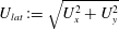 $U_{lat}:=\sqrt{U_{x}^{2}+U_{y}^{2}}$
, (b)) and rise velocity (c). The red vertical lines indicate the instances in time shown in figure 24.

Figure 30 depicts the single-sided amplitude spectra of the discrete Fourier transforms of the velocity against the spherical harmonics coefficients
 $c_{0}^{0}$
and
 $c_{2}^{0}$
; cf. figure 36 for the associated time signals.
Single-sided amplitude spectra of spherical harmonics coefficient
 $c_{2}^{0}$
and terminal velocity
 $U_{t}$
for 14 mm (a) and 16 mm droplet (b).

The lateral velocity components of both droplets show a clear peak at about 0.75 Hz, corresponding to Strouhal numbers of
 $\mathit{St}_{14}=0.106$
and
 $\mathit{St}_{16}=0.129$
. The discrete Fourier transformation of the spherical harmonics coefficients shows a peak at twice that frequency.
At the moment of highest skewness, the
 $x$
- and
 $y$
-extents of the droplet are smallest, whereas the
 $z$
-extent has a maximum. This happens twice in each vortex shedding cycle. Therefore the frequencies encountered in the shape data are twice as high as those of the velocity data. This can be understood by considering the rocking droplet motion in a plane: in every complete sequence of rocking, there are two minima of the shape data, denoted by 2 and 4 in figure 24.
The rocking movement is accompanied by periodic vortex shedding as depicted in figures 31 and 32. For both droplets, a full sequence of rocking is accompanied by the shedding of two vortex rings. Therefore, the vortex shedding takes place with the same frequency as the rocking motion.
Vortex shedding of 14 mm droplet. The
 $-10$
Pa iso surface of pressure is shown over a time span of 1.3 s, corresponding to oscillations at about 0.75 Hz.

Vortex shedding of 16 mm droplet. The
 $-15$
Pa iso surface of pressure is shown over a time span of 1.5 s, corresponding to oscillations at about 0.7 Hz.

It is interesting that the frequency in both cases is almost identical. A similar observation has been made in Lunde & Perkins (Reference Lunde and Perkins1998), where it was found experimentally that the vortex shedding frequency of air bubbles rising in tap water is independent of
 $\mathit{Re}$
.
Shape analysis
As previously discussed, the residuals of the shape description in table 7 show that the suitability of the bi-ellipsoid description has reached its bounds for droplets larger than 10 mm. Figure 33 depicts the angular decomposition of the first principal axis
 $\boldsymbol{t}_{3}$
and the centre of mass velocity over time, which again show overall good agreement. However, contrary to the smaller droplets, there is a distinguishable backward phase shift of the principal axis polar and azimuthal angles, accompanied by an amplitude deviation of the azimuthal angle. This indicates that the path changes follow the shape changes with a slight delay, due to the stronger influence of inertia.
Azimuthal (
 ${\it\theta}$
) and polar (
 ${\it\varphi}$
) angle of principal axis
 $\boldsymbol{t}_{3}$
(
 ${\it\theta}$
: ○,
 ${\it\varphi}$
: ▫) and droplet centre velocity (
 ${\it\theta}$
: solid,
 ${\it\varphi}$
: dashed) for 16 mm droplet (
 $d/({\rm\Delta}x)=60$
).

The droplet undergoes several quarter polar rotations, which go back and forth over time, accompanied by azimuthal oscillations with a frequency of 0.71 Hz. The agreement with the first principal axis decreases, since the amplitudes of the azimuthal angle deviate more strongly. This is an indication of surface oscillations, which exhibit a slight backward phase shift with respect to the path oscillations.
Interface of 14 mm droplet (
 $d/{\rm\Delta}x=72$
) reconstructed from spherical harmonics.

Droplet interface of 14 mm droplet (
 $d/{\rm\Delta}x=72$
) projected (convex hull) to the Cartesian planes (solid) and principal planes (dashed,
 $T_{ij}=\text{span}\{\boldsymbol{t}_{i},\boldsymbol{t}_{j}\}$
) (coordinates in
 $d$
) for
 $t=4~\text{s}$
(a–c) and
 $t=10~\text{s}$
(d–f): (a,d)
 $xy$
and
 $T_{12}$
, (b,e)
 $xz$
and
 $T_{13}$
, (c,f)
 $yz$
and
 $T_{23}$
.

Spherical harmonics coefficients
 $c_{2}^{0}$
(solid) and
 $c_{2}^{2}$
(dashed) for 16 mm droplet.

6. Conclusion
The paper initiates a systematic computational analysis of the rise dynamics of high viscosity droplets in a viscous ambient liquid, considering a system of corn oil droplets rising in pure water. For this purpose, detailed, fully three-dimensional numerical simulations using the in-house VOF-code FS3D have been performed for a series of corn oil droplets of different diameter, ranging from 0.5 to 16 mm. Reliable simulation results require small time steps and a balanced surface tension force calculation, especially in order to treat small droplets of 1 mm radius or below. The time step constraints are particularly severe because of the high particle viscosity in conjunction with the explicit time discretization used here.
Resolution requirements are challenging due to the complex droplet dynamics, in particular for larger drops. Even so, convergence of integral quantities such as the terminal rise velocity for steady rise, or locally averaged rise velocities and principal frequencies in oscillatory cases, have always been obtained, and the qualitative rise dynamics are captured.
Similar to the rise or fall of rigid spheres and bubbles, the simulations reveal a fascinating bifurcation scenario which governs the route to increasingly complex and dynamical flow fields with increasing droplet diameter. The main qualitative rise dynamics are summarized in figure 37 in their relation to the terminal rise velocity. It can be clearly seen how every single bifurcation, accompanied by a further loss of symmetries, decreases the slope of the initially linear relationship between the terminal velocity and the droplet diameter. This leads to a sublinear growth up to a maximum velocity which is attained for the 10 mm droplet. At this point, vortex shedding and path oscillations of significant and increasing amplitude result in a decrease of the terminal rise velocity, with an inclination point somewhere between 12 and 14 mm. The rise velocity then appears to reach a plateau, but proof of this requires further study for larger drops – which will tend to break up above a certain diameter.
Rise velocity and characteristics versus droplet diameter.

Coming back to the questions raised in the introduction, we now have the following picture:
-
(i) The onset of a wavy wake and vortex shedding is already observed for the oscillatory oblique regime of the 3.7 mm droplet. Moreover, vortex shedding occurs in the intermittent oblique regime when the droplet changes its direction. The rise paths in the latter regime are also slightly oscillatory, but these minor oscillations are uncorrelated with the vortex shedding. With increasing diameter, the shape of the droplets is deformed from spherical to an oblate ellipsoid of increasing eccentricity, followed by bi-ellipsoidal shapes with significantly higher curvature on the back side of the droplet. Nevertheless, significant shape oscillations are only observed for diameters of 14 and 16 mm, i.e. only for droplets much larger than those which display oscillatory paths.
-
(ii) We clearly detected the occurrence of a steady oblique rise path for the 3.2 mm droplet. This is in a way consistent with the results from Horowitz & Williamson (Reference Horowitz and Williamson2010), where freely rising or falling rigid spheres have been studied and their regime map figure 27 displays a large range of Reynolds numbers from 210 to 600 in which oblique rise or fall occurs for density ratios above 0.35. This is followed by a range of intermittent oblique rise up to
$\mathit{Re}=1550$
. It seems reasonable that these regimes are somewhat shifted towards smaller Reynolds numbers for deformable fluid particles. In our study of rising high viscosity droplets, we observed oblique rise for
$\mathit{Re}=198,251$
(as opposed to steady rise at
$\mathit{Re}=134$
) and intermittent oblique rise for
$\mathit{Re}=311,496,849$
(as opposed to an essentially vertical, oscillatory rise at
$\mathit{Re}=1150$
). -
(iii) In contrast to the rise behaviour of bubbles, helical paths are not observed in the present study. The oscillatory rise paths of the largest considered corn oil drops is best described as zigzagging, but the bifurcation scenario leading there appears to be completely different from that leading to zigzagging of air bubbles. In particular, the lateral extent to which the droplets move is smaller than one droplet diameter. Therefore, this regime seems closely related to the second regime of straight rise in Horowitz & Williamson (Reference Horowitz and Williamson2010). It seems reasonable that the deformable interface, and the flat shape of the droplet at such high Reynolds numbers, are a necessary prerequisite for the oscillatory behaviour observed here.




The approach via detailed three-dimensional numerical simulations with a freely deforming interface allows for the investigation of local field data which are hard to access by measurements. Using these local data, our main findings are: (a) the combination of the approximate solution for the flow field due to Taylor and Acrivos with the simulated rise velocity yields a good agreement of the velocity field for the smallest droplet; (b) for droplets rising on intermittently oblique paths, an intermittent bifid wake with alternating vorticity is generated; (c) the wake structures change drastically for the different droplet sizes, deadzones (i.e. regions of exceedingly low flow) can occur in the wake and even the transport of vortex structures upwards within the wake is observed; (d) shape oscillations lead to velocity oscillations with strongly correlated dynamics; (e) vortex shedding from the largest droplets (diameter of 14 and 16 mm) is accompanied by a complex evolution of coherent vortex structures connecting the droplet to the shed vortices.
The subject of high viscosity droplet dynamics deserves and requires further investigation. Of particular interest would be the identification of the critical Reynolds numbers using a computer assisted global linear stability analysis in the spirit of Albert, Tezuka & Bothe (Reference Albert, Tezuka and Bothe2014).
Acknowledgements
C.A. and D.B. are grateful for financial support by the Deutsche Forschungsgemeinschaft (DFG) within the cluster of excellence Center of Smart Interfaces (CSI) at the Technische Universität Darmstadt. The work of J.K. is supported by the Excellence Initiative of the German Federal and State Governments and the Graduate School of Computational Engineering at the Technische Universität Darmstadt. A.M.R. would like to thank the DFG for hosting her collaborative visit for work on this project at the CSI during the period of 1–30 June 2010.
We wish to thank the late Martin Schmidtke for proving the principal feasibility of direct numerical simulations for high viscosity oil droplets in water employing the VOF code FS3D.