1 Introduction
Choosing the best word or phrase for a given context from among the candidate near-synonyms is a difficult language generation problem. While Natural Language Generation (NLG) systems do have to consider lexical choice in general, it is typically not at the level of the fine distinctions embodied in near-synonyms. These can be important, as noted by Inkpen and Hirst (Reference Inkpen and Hirst2006), who describe an NLG system that incorporates a knowledge base of near-synonym differences: for example, the choice between the flattering slim and the less complimentary skinny is significant. Extensions of this general idea of focussing on near-synonyms include systems that can rewrite text to be more positive or more negative (Inkpen, Feiguina, and Hirst Reference Inkpen, Feiguina, Hirst, Shanahan, Qu and Wiebe2006) – for example, as an email filter to soften a potentially inflammatory first draft, or as an intensifier for an opinion piece intended to persuade – or an intelligent thesaurus that can help a writer by ordering proposed word choices by the suitability of the context (Inkpen Reference Inkpen2007a). In the language generation context, it is clear that a full-featured system would need to handle the problem of choosing among near-synonyms or paraphrases in order to select the most felicitous phrasing and at times to avoid serious errors in language production.
The first task defined to explore this problem is the near-synonym lexical gap problem formalised by Edmonds (Reference Edmonds1997), Footnote 1 more recently termed the Fill in the Blanks (FITB) task, in which a word is removed from a sentence of text, and a system is offered both the original word and some of its near-synonyms as potential replacements. Edmonds offers this example of the task, in which the system must choose which of error, mistake or oversight fits into the gap in this sentence:
(1) However, such a move also would run the risk of cutting deeply into U.S. economic growth, which is why some economists think it would be a big ________.
Edmonds used an unsupervised approach, testing it on seven sets of synonyms (synsets) from WordNet (Fellbaum Reference Fellbaum1998). This work was extended by Inkpen (Reference Inkpen2007b), who used much more training data and a language model in an alternative unsupervised approach, which had much better results on Edmonds’s test set. Gardiner and Dras (Reference Gardiner and Dras2007a, Reference Gardiner and Drasb), looking at a larger test set (fifty-eight synsets versus seven), found that affective near-synonyms (for example bad, insecure, risky . . .) and non-affective near-synonyms behave differently, and suggested that near-synonyms with affective differences might be amenable to different techniques from those that are effective for non-affective near-synonyms.
In this paper, we explore this suggestion, drawing on work in sentiment analysis. First, we investigate a supervised approach; as in the first exploration of supervised methods in document sentiment classification, by Pang, Lee and Vaithyanathan (2002), we start with a simple unigram model. Second, we then look at broader aspects of the document to use as features. We hypothesise that affective differences between near-synonyms, such as the difference in attitude between slim and skinny, may be more influenced by more general aspects of the document such as affect, than are near-synonyms that differ in other aspects. We test this hypothesis by applying proven techniques from the domain of sentiment analysis (Pang et al. Reference Pang, Lee and Vaithyanathan2002) to the FITB problem, while investigating some new feature types for this problem combined with feature weighting techniques.
In Section 2, we discuss some related work on lexical replacement and (briefly) on sentiment analysis; in Section 3, we describe our data; and in Section 4, we discuss the selection of appropriate baselines. In Section 5, we describe our experimental setup, followed by the definition of our unigram models. We discuss the results of these, which motivates the selection of some further features. Section 6 then describes further experiments based on the document-level features arising from Section 5, while Section 7 describes those based on a notion of weighting in the feature space.
2 Related work
While lexical selection is an issue in several applications that involve computational production of language – for example, Machine Translation (MT) – we only focus on the work that has been motivated by the task of NLG (Reiter and Dale Reference Reiter and Dale2000). In MT, for example, any choosing among near-synonyms that occurs is an implicit part of the overall statistical model; Footnote 2 in the NLG-motivated work we look at, choosing among near-synonyms has been framed as an explicit problem, the FITB task, which we discuss below.
2.1 Lexical selection in NLG
The FITB task has been directly addressed by several authors. It was introduced by Edmonds (Reference Edmonds1997), who experimented with seven sets of near-synonyms – for example, one set consists of the words responsibility, burden, obligation, and commitment – and describes a statistical system which can predict the original choice of wordFootnote 3 55.7% of the time depending on a chosen set of near-synonyms, according to the aggregate figures of Inkpen (Reference Inkpen2007b). Edmonds (Reference Edmonds1999) reports an extension to all WordNet synsets, in which the precision is 74.5% against a most-frequent baseline of 73.3%. Inkpen (Reference Inkpen2007b), taking a supervised approach using Pointwise Mutual Information (PMI) scores of the left and right context and the presence of frequent words in the context, reports an ability to predict the author’s original choice of word of about 66% overall on Edmonds’ original seven hand-chosen test cases, an improvement over the baseline of about 20%.
Following these, several alternative approaches have been proposed. Islam and Inkpen (Reference Islam and Inkpen2010) used a language model built using data from the Google Web1T corpus (Brants and Franz Reference Brants and Franz2006). Wang and Hirst (Reference Wang and Hirst2010) used Latent Semantic Analysis (Landauer and Dumais Reference Landauer and Dumais1997) – drawing on the success of Rapp (Reference Rapp2008) on a related task, that of identifying potential synonyms rather than choosing the usage of them – to perform dimensionality reduction on the feature space, and compare document representations with context representations. Yu et al. (Reference Yu, Shih, Lai, Yeh and Wu2010) use feature values derived from the Google Web1T corpus as suggested in Gardiner and Dras (Reference Gardiner and Dras2007b), weighting feature values by the strength of the collocation with given near-synonyms. Islam (Reference Islam2011) proposed a two-phase method, categorising n-grams based on the position of the candidate word to fill in the blank within the n-gram, and defining a normalised frequency to rank candidates. All of these approaches were evaluated on the Edmonds set of seven test cases; all produced higher results, with the last of these, Islam (Reference Islam2011), reaching 75.4%.Footnote 4
The FITB task is closely related to the lexical substitution task addressed at SemEval-2007 (McCarthy and Navigli Reference McCarthy and Navigli2007). In this task, instead of being presented with a gap and being required to correctly predict the author’s original word choice from among several alternatives, the systems are given the author’s original word choice and asked to predict a suitable alternative; the gold standard is a set of alternatives that came from a human annotation exercise carried out by the task organisers. Further, unlike in the FITB task, the set of alternative words is not fixed. The results of this harder task are not directly comparable to the FITB task, and the ability of systems to predict the very best alternative word had precision and recall of not greater than 13%. Baseline systems derived from walking the WordNet hierarchy around a target word performed at about 10% precision and recall whereas a distributional similarity baseline performed at under 9% precision and recall.
The methods used by the two best performing lexical substitution systems on the task requiring the best single substitute, as ranked by McCarthy and Navigli (Reference McCarthy and Navigli2007), were: a language model trained on the 1012 words of the Web1T 5-gram dataset (Brants and Franz Reference Brants and Franz2006) selecting from words drawn from all WordNet synsets of the target word and all neighbouring synsets (Yuret Reference Yuret2007); and a voting system between several selection methods including a language model, a machine translation test and a Latent Semantic Analysis measure selecting words drawn from several sources including WordNet and Microsoft Encarta (Hassan et al. Reference Hassan, Csomai, Banea, Sinha and Mihalcea2007). The major explanation for the considerably lower performance reported by the best systems on the lexical substitution task as opposed to the FITB task is presumably the number of substitutes that the lexical substitution systems consider, none of which is guaranteed to be the correct replacement. In the FITB task, typically systems are considering between three and seven possible substitutes, and the correct replacement is guaranteed to be among them. A very recent investigation of various approaches to the lexical substitution task with multiple lexical resources can be found in Sinha and Mihalcea (Reference Sinha and Mihalcea2014).
2.2 Sentiment and subjectivity analysis
Sentiment analysis and the closely related field of subjectivity analysis is a field concerned with predicting the sentiment features of text. There are several major tasks: determining the overall opinion of a text such as a review and identifying and classifying parts of the document with their own sentiment; identifying subjective elements within a piece of text; identifying differing opinions within a text in, for example, a review with multiple parts; and identifying features within documents that contribute to overall subjectivity or sentiment classification.
In the task of determining the overall opinion, the goal is to predict, or, in evaluating, re-predict a sentiment label assigned to a text. For example, a movie review might rate a movie as nine out of a possible ten. The task then is, given the text of the review, to re-assign the correct label. The label may be fine-grained (correctly predicting a score of nine out of seven) or coarse-grained (correctly predicting whether a review is positive or negative). Examples of approaches to this task include the unsupervised method of Turney (Reference Turney2002) inferring the individual sentiment values of words and using these to predict the sentiment of movie reviews; the exploration by Pang et al. (Reference Pang, Lee and Vaithyanathan2002) of various machine learning approaches to the problem of classifying movie reviews; and the application by Gamon (Reference Gamon2004) of machine learning techniques to a domain more difficult than movie reviews, customer feedback data. As an extension of this problem, some authors have examined determining the sentiment of different aspects of a document. For example, Snyder and Barzilay (Reference Snyder and Barzilay2007) examine the ranking of different aspects of a restaurant review, such as food and ambience.
A partially separate strand of investigation is subjectivity analysis, fundamentally although not exclusively concerned with distinguishing subjective text expressing the private viewpoint of an actor from objective text. It may be concerned with identifying subjective parts of a single document as in Hatzivassiloglou and Wiebe (Reference Hatzivassiloglou and Wiebe2000) and Wiebe et al. (Reference Wiebe, Wilson, Bruce, Bell and Martin2004), or, as Pang and Lee (Reference Pang and Lee2008) explain, as a variety of genre classification into the genres of ‘editorial’ and ‘news’, giving examples such as Yu and Hatzivassiloglou (Reference Yu and Hatzivassiloglou2003) and many following.
The two strands of research often make use of similar features, or each others’ results. For example, Pang and Lee (Reference Pang and Lee2004) found that identifying subjective portions of a document could result in more accurate classifications of the overall sentiment of the original review.
3 Affective text: near-synonyms and corpora
As noted in Section 1, our focus is on the FITB task, and the characteristics of the candidate near-synonyms that might fill the gap. Various typologies for near-synonyms, in terms of the differences in nuance that they can embody, have been proposed; following are the distinctions made by, and terminology used by, three such typologies:
• semantic or denotational variation (mist and fog) and stylistic or connotational variation (stingy and frugal) — DiMarco, Hirst and Stede (Reference DiMarco, Hirst and Stede1993);
• collocational and syntactic variations (die and pass away), stylistic variations (house and habitation), expressive variations (skinny and slim) and denotational variations (error, blunder and mistake) — Edmonds and Hirst (Reference Edmonds and Hirst2002); and
• denotational differences (invasion and incursion), attitudinal variations (placid and unimaginative) and stylistic differences (assistant and helper) — Edmonds and Hirst (Reference Edmonds and Hirst2002) and Inkpen and Hirst (Reference Inkpen and Hirst2006).
We are just interested in a broader classification, into either affective or non-affective, as in our earlier work of Gardiner and Dras (Reference Gardiner and Dras2007a, Reference Gardiner and Drasb): whether the near-synonyms differ in sentiment expressed towards their subject, or whether they differ in some other way.
In this paper, we explore the idea that affective and non-affective synonyms might behave differently in the context of the FITB task. To do this, we require both a set of near-synonyms and a set of documents with known document sentiment. Our choice of these two datasets is described in the following subsections.
3.1 Documents containing sentiment
As samples of our test words in context, and a standard source of affective text, we took the widely used Movie Review Corpus sentiment scale data set, version 1.0 (Scale 1.0) introduced by Pang and Lee (Reference Pang and Lee2005). The data consists of movie reviews authored by four reviewers on Internet sites, ranging from extremely negative to extremely positive reviews (there are 5,000 short reviews in total, average length around 380 words). Scores are given on a 10-point scale, normalised to the range [0,1]; the label ‘positive’ in this data is assigned to scores ⩾ 0.7, and the label ‘negative’ is assigned to scores ⩽ 0.4. This score is available as the rating attribute of each review.Footnote 5
3.2 Sentiment annotated near-synonyms
Since we seek to examine the choice between near-synonyms that differ in sentiment we require a source of such near-synonyms. There are several sources of near-synonyms not annotated for polarity: the major one used in previous work was WordNet (Fellbaum Reference Fellbaum1998) used by Edmonds (Reference Edmonds1997), Inkpen (Reference Inkpen2007b) and Gardiner and Dras (Gardiner and Dras Reference Gardiner and Dras2007a, Reference Gardiner and Drasb) to test their near-synonym usage prediction methods. However, not only is WordNet not annotated for polarity, it encodes very fine-grained sense distinctions which usually precludes having near-synonyms that differ in sentiment contained in a single synset. In addition, there were very few synsets – only seven of the fifty-eight used in the Gardiner and Dras work – that had any affective meaning, and as we are especially interested in these sets, we require an additional source of near synonyms. Footnote 6
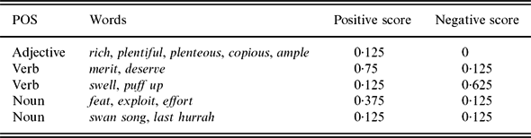
There are some versions of WordNet annotated for sentiment, for example SentiWordNet (Esuli and Sebastiani Reference Esuli and Sebastiani2006), but examination of this data shows that it is not easy to use it to produce clear distinctions such as ‘this set of near-synonyms differ in sentiment and these do not’. As an example of why SentiWordNet is a difficult source of data for this use-case, consider the five entries from it shown in Table 1. While having real-numbered values for the positivity and negativity of synsets would be of use if we were seeking features for a sentiment classification learner, one of the uses to which SentiWordNet has been put, it is not straightforwardly apparent how to identify ‘synsets that have the same affect’, ‘synsets that differ in affect’ and ‘synsets that have no affective meaning’ from the numerical values.
Example entries from SentiWordNet

There are other resources such as the General Inquirer word list (Stone et al. Reference Stone, Dunphy, Smith and Ogilvie1966) which have been human-annotated with sentiment, but which are not already grouped into near-synonym sets, and are only concerned with polarity, rather than degrees of sentiment.
The near-synonym usage guide Choose the Right Word (Hayakawa Reference Hayakawa1994) contains near-synonym sets chosen by a human author specifically as a guide to the subtleties of near-synonym word choice for readers and writers of English. It is therefore a good source of near-synonyms that differ in fundamental ways such as sentiment. It was used by Inkpen and Hirst (Reference Inkpen and Hirst2006) as a source of near-synonyms marked for differences such as denotational differences (in which near-synonyms could differ in what they suggest or imply, for example) and attitude and style differences, including near-synonyms that are more pejorative, disapproving or favourable. In addition, unlike resources such as SentiWordNet, it has explicit characterisations of the differences between the near-synonyms.
Inkpen and Hirst (Reference Inkpen and Hirst2006) derived data automatically from Choose the Right Word by a decision list algorithm, and this data is not available for reasons of copyright. In addition, the focus of this data was on all axes in which near-synonyms can differ, rather than on the axis of positive or negative attitude to the subject of a description in particular. Thus we have annotated our own data.
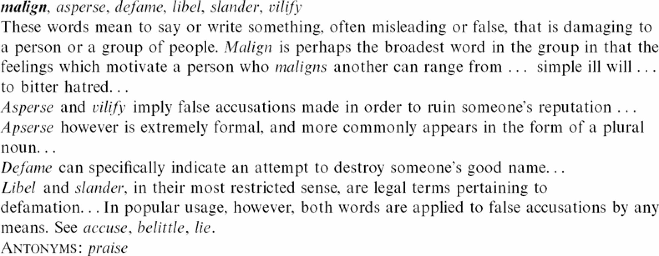
We use sets of near-synonyms drawn from an earlier edition of this work, Use the Right Word (Hayakawa Reference Hayakawa1968). (An excerpt from an entry in Use the Right Word is shown in Figure 1 as an example of its contents.Footnote 7) As a first pass, we sampled the sets by annotating those that are listed under the letter A, of which there are fifty-seven in total. Of these fifty-seven total sets, we exclude sixteen sets that do not include at least two words that are each used at least five times in our sentiment annotated documents described in Section 3.1. This left thirty-seven sets, totalling 133 words. Because this dataset only contained five sets with the same affect shared among all words (see annotation description immediately following), we added an extra ten sets (also from Use the Right Word, but beyond the letter A) with the same affect shared among all the words to balance the number of test sets.
Excerpt from an entry in Use the Right Word.

We thus have a total of forty-seven test sets. These near synonyms were annotated for affect by one of the authors. The annotation scheme called on the annotator to rely on Use the Right Word's interpretation of the sets, rather than personal linguistic intuition. For example, Use the Right Word suggests in the entry for aloof : ‘Both reserved and detached can be associated with attractive qualities, whereas aloof is seldom so considered’. Annotations were of two kinds:
(1) for a given set, whether Use the Right Word indicates that that set contains at least some words conveying sentiment (‘affective’, or ‘not affective’); or
(2) for every word within any set marked as ‘affective’, whether Use the Right Word indicates that that word has positive, negative, or neutral affect.
Near-synonym sets were then given one of three labels: no-affect, for those where no element of the set conveyed sentiment; same-affect, for those which contain only positive or only negative words (not neutral ones); or differing-affect, where the words contained different sentiment. (Note that differing-affect sets can contain neutral words, such as the set consisting of positive insight and neutral perception.)
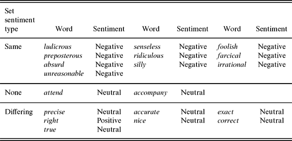
An example of three annotated test sets is shown in Table 2. Observe that the set containing attend and accompany has set type marked as None, meaning no affect. The marking of Neutral against the individual words is thus implied. The set containing ludicrous, senseless and others is marked Same, and all the words are indeed marked identically with Negative sentiment. The set containing precise, accurate and others is marked Differing and the sentiment of the individual words does indeed differ, with words within it having varying Positive and Neutral sentiment. The complete set of annotated near synonym sets is given in Appendix A.
Examples of test sets annotated for overall set sentiment differences, and for the sentiment of individual words
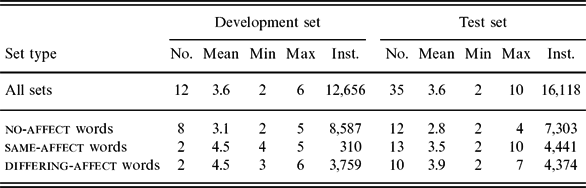
We divided the sets into development and test data; examples were inspected from the development data during development of the models. The distribution of near synonym sets is then shown in Table 3. The number of instances used in our evaluation (development set: 12,656; test set: 16,118) is comparable to the classic Reuters-21578 corpus used in text classification (21,578 instances) or the development and test sets used in the 2013 Workshop on Machine Translation shared task.Footnote 8
Distribution of sentiment among Use the Right Word sets in Scale 1.0 corpus: number of sets with a particular sentiment; mean, minimum and maximum number of words in sets; number of instances
4 Comparison of baselines
There are a number of possible baselines, each with various merits. As candidates in this paper, we consider two standard approaches (most frequent category, and a language model-based one); and two based on methods published in the literature, those of Edmonds (Reference Edmonds1997) and Inkpen (Reference Inkpen2007b), for which we use the implementations described in Gardiner and Dras (Reference Gardiner and Dras2007a) and Gardiner and Dras (Reference Gardiner and Dras2007b) respectively. We will here refer to those implementations as Edmonds-collocate and Web1TPMI.
We outline these below, and discuss their relative performance, along with the resulting choice of baseline for the rest of the paper.
4.1 Candidate baselines
4.1.1 Most frequent
With respect to baselines, Edmonds (Reference Edmonds1997) and Inkpen (Reference Inkpen2007b) both use a most frequent baseline, that is, comparing with the method of always selecting the most frequent word in a set to fill the gap. This baseline can be quite high: Inkpen reports it as achieving 44.8% accuracy on the seven sets of test words used by herself and Edmonds (these seven sets contain between two and four words, with a mean of exactly three words per set). However, we find that on our dataset, even the most-frequent baseline is considerably higher for most sets in our development set, as shown in Table 4.
Percentage point increase of alternative baselines over most frequent baseline
4.1.2 Language model
As Inkpen (Reference Inkpen2007b) notes, and as seen in the 2007 lexical substitution task, statistical language models are the mainstream method of lexical choice. Inkpen and Hirst (Reference Inkpen and Hirst2006) compared their system to a language model baseline that was implemented as part of the HALogen NLG system (Langkilde and Knight Reference Langkilde and Knight1998), trained on 250 million works of text from the news genre. HALogen’s word choices when combined with the anti-collocation method presented by Inkpen and Hirst (Reference Inkpen and Hirst2006) outperformed HALogen alone, and the method presented by Inkpen (Reference Inkpen2007b) outperforms anti-collocations, and thus Inkpen (Reference Inkpen2007b) concludes that language models would be outperformed by her newer method.
Here we implement a baseline language model choice system using the Web1T data (Brants and Franz Reference Brants and Franz2006). Web 1T contains n-gram frequency counts, up to and including 5-grams, as they occur in a trillion words of World Wide Web text. There is no context information beyond the n-gram boundaries. Examples of a 3-gram and a 5-gram and their respective counts from Web 1T are shown in examples (2) and (3):
(2)

(3)


We make a word choice by estimating the most probable 3-gram,Footnote 9 backing off to 2-grams and 1-grams where necessary. We fundamentally use the backoff method of Katz (Reference Katz1987). The standard approach to Katz uses smoothing below some threshold to avoid data sparseness for low-frequency items, with this threshold often empirically determined, and uses the more accurate raw high-frequency accounts above it. Given that Web1T only provides counts frequencies of at least forty for bi- to 5-grams and 200 for unigrams, we use these as our threshold. Full details of our adaptation of Katz to the Web1T data are given in Appendix B.
4.1.3 Edmonds-collocate prediction method
Here we describe our implementation of Edmonds (Reference Edmonds1997). For the gap in sentence S, each candidate token c – where a token is a part-of-speech tagged word, such as (JJ arduous) or (NN fight) – is assigned a score, score(c, S), which is the sum of its significance score with each individual remaining token w in that sentence.
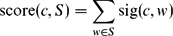 \begin{equation}
\textrm {score}(c,S) = \sum _{w\in S} \textrm {sig}(c, w)
\end{equation}
The candidate c which maximises score(c, S) is chosen as the word fitting the lexical gap in sentence S.
Edmonds computed the score sig(c, w) by connecting words in a collocation network. The principle is that if word w 0 co-occurs significantly with word w 1 which in turn co-occurs significantly with word w 2, then the presence of w 0 should weakly predict the appearance of w 2 even if they do not significantly co-occur in the training corpus. That is, he assumes that if, for example, task co-occurs significantly with difficult, and difficult co-occurs significantly with learn, then task and learn should weakly predict each other’s presence.
Edmonds proposes extending this technique to co-occurrence networks with prediction chains of arbitrary length, but his experimental results suggest that in practice two connections approaches the limit of the usefulness of the technique. Therefore, to compute sig(c, w) we take the shortest path of significance between the tokens c and w, which is either c, w where c and w significantly co-occur, or c, w 0, w where c and w both significantly co-occur with a third word, w 0.
Where tokens c and w significantly co-occur together, their significance score is their t-score (Church et al. Reference Church, Gale, Hanks, Hindle and Zernick1991), which we calculate by the N-gram Statistics Package (Banerjee and Pedersen Reference Banerjee and Pedersen2003):
 \begin{equation}
\textrm {sig}(c, w) = t(c, w)
\end{equation}
The t-score is calculated by comparing the likelihood of both words c and w occurring within a certain window of each other. The size of the window is either a 4 word window surrounding c, that is, c and w were found at most two words apart, or a ten word window surrounding c, that is, c and w were found at most five words apart.
Where tokens c and w both significantly co-occur with token w 0, their significance score is a combination of their t-scores, with a bias factor devised by Edmonds to account for their weaker connection.
 \begin{equation}
\textrm {sig}(c, w) = \frac{1}{8}\left(t(c,w_{0}) + \frac{t(w_{0}, w)}{2}\right)
\end{equation}
If there is more than one candidate word w 0 co-occurring significantly with both c and w, the word w 0 is chosen so that the value of sig(c, w) in (6) is maximised.
Where more than one candidate word c maximises sig(c, w) or where sig(c, w) = 0 for all candidate words c, we back off to the baseline result of the most frequent word.
In the above, we have used ‘significantly co-occur’ without definition. The test we are using is that from the description by Edmonds (Reference Edmonds1999) of the same experiment: any two words w 0 and w 1 significantly co-occur if their t-scores are greater than 2.0 and their mutual information score is greater than 3.0, as suggested by the observation of Church et al. (Reference Church, Gale, Hanks, Hindle and Zernick1991) that t-scores and mutual information scores emphasise different kinds of co-occurrence.
Input to the t-score and mutual information systems was the part-of-speech tagged 1989 Wall Street Journal, as in Edmonds’s work. Stop words were those used by Edmonds, defined as any token with a raw frequency of over 800 in the corpus, and all punctuation, numbers, symbols and proper nouns. As per Edmonds we did not perform lemmatisation or word sense disambiguation.
4.1.4 Web1TPMI prediction method
In the near-synonym prediction method described by Inkpen (Reference Inkpen2007b), here called Inkpen-PMI, the suitability of candidate c for a given gap is approximated differently from Edmonds-collocate: the entire sentence is not used to measure the suitability of the word. Instead, a certain sized window of k words either side of the gap is used. For example, if k = 3, the word missing from the sentence in example (7) is predicted using only the six words shown in example (8).
(7) Visitors to Istanbul often sense a second, ________ layer beneath the city's tangible beauty.
(8) sense a second, ________ layer beneath the
Given a text fragment f consisting of 2k words, k words either side of a gap g (w 1, w 2, . . ., wk, g, w k + 1, . . ., w 2k), the suitability s(c, g) of any given candidate word c to fill the gap g is given by
 \begin{equation}
s(c,g)=\sum _{j=1}^{k}PMI(c,w_{j})+\sum _{j=k+1}^{2k}PMI(w_{j},c)
\end{equation}
Inkpen-PMI estimates the token counts for PMI(x, y) by issuing queries to the Waterloo MultiText System (Clarke and Terra Reference Clarke and Terra2003) for occurrences of x and y separately and within a query frame of length q within a corpus.
According to Inkpen (Reference Inkpen2007b), Inkpen-PMI outperformed both the baseline and Edmonds-collocate by 22 and 10 percentage points respectively on the seven synsets from Edmonds (Reference Edmonds1997).
In this work, without access to the Waterloo Multitext System and the corpus used by Inkpen, we require an approximation to the method. Web1TPMI, our variation on Inkpen-PMI, is designed to estimate PMI(x, y), the pointwise mutual information of words x and y, using the Web 1T 5-gram corpus Version 1 (Brants and Franz Reference Brants and Franz2006) (described in Section 4.1.2).
The n-gram counts of Web1T allow us to estimate the occurrence of x and y within a query frame k by summing the Web 1T counts of k-grams in which words x and y occur and x is followed by y. Counts are computed using the Web 1T processing software ‘Get 1T’ detailed in Hawker, Gardiner and Bennetts (Reference Hawker, Gardiner and Bennetts2007). Queries are matched case-insensitively, but no stemming takes place, and there is no deeper analysis (such as part of speech matching).
This gives us the following methodology for a given lexical gap g and a window of k words either side of the gap:
(1) for every candidate near-synonym c:
(a) for every word wi in the set of words preceding the gap, w 1, . . ., wk, calculate PMI(wi, c), given counts for occurrences of wi, c and wi and c within a query frame from Web 1T;Footnote 10
(b) for every word wj in the set of words following the gap, w k + 1, . . ., w 2k, calculate PMI(c, wj) as above;
(c) compute the suitability score s(c, g) of candidate c as given by (9);
(2) select the candidate near-synonym with the highest suitability score for the gap where a single such candidate exists;
(3) where there is no single candidate with a highest suitability score, select the most frequent candidate for the gap (that is, fall back to the baseline described in Section 4.1.1).Footnote 11
Since Web 1T contains 5-gram counts, we can use query frame sizes from q = 1 (words x and y must be adjacent, that is, occur in the 2-gram counts) to q = 4.
4.2 Results and discussion
We discuss each individual potential baseline with respect to the most frequent baseline below. In summary, all performed worse, so we use the most frequent baseline in the rest of the paper. Comparative results of all candidate baselines are shown in Table 4.Footnote 12, Footnote 13
4.2.1 Language model results
The language model badly underperformed compared to the most frequent baseline, which was not expected from the results of Inkpen and Hirst (Reference Inkpen and Hirst2006). It is, however, difficult to compare this result directly with the one given in Inkpen and Hirst (Reference Inkpen and Hirst2006). In that article, the HALogen system's language model, which predicts the correct near-synonym between 58% and 83% of the time, is given as a baseline against which to compare the Xenon experimental system, but values for the most frequent baseline are not given for the same test sets.
One possible reason for the bad performance of the language model is that the most frequent baseline here, as noted earlier, is substantially higher than in other work; perhaps there is something about the nature of our near-synonym sets. A second possible reason that could interact with the first is suggested by Inkpen and Hirst (Reference Inkpen and Hirst2006), who note that the collocations encoded in the language model will tend to be with function words, per the short n-gram distance. However, in light of the good performance of language models on the FITB task described in Islam and Inkpen (Reference Islam and Inkpen2010), also trained on Web1T, this would be worth investigating further. There are some differences in our language model implementation to that of Islam and Inkpen (Reference Islam and Inkpen2010), including a different smoothing technique and the use of 3-grams rather than 5-grams. However, without a high performing language model, we do not consider it as a baseline in this work.
4.2.2 Edmonds-collocate results
Table 4 includes results for Edmonds-collocate where the query window size is four. Results for query window size ten are generally very slightly worse again. In fact, the method only makes predictions for at most 10% of the time (and for some of the sets, makes no predictions at all): the backoff strategy accounts for its relative closeness to the most frequent baseline. This is unsurprising given the finding that Edmonds-collocate simply does not use a large enough training set to make useful predictions (Inkpen Reference Inkpen2007b).
4.2.3 Web1TPMI results
The best performance for Web1TPMI parameters was q = 2 and w = 2, which are shown in comparison with other baselines in Table 4. One noteworthy characteristic of the varying parameters is that a wider window (parameter k) of context around a gap almost always diminishes performance.
In general these results also show a large decrease in performance over the baseline, contrary to results reported in Gardiner and Dras (Reference Gardiner and Dras2007b), where results were approximately equal to the baseline. Several reasons may hold as to why Web1TPMI performs unexpectedly poorly. First, the movie review test data in this article is very different from that used in Gardiner and Dras (Reference Gardiner and Dras2007b), which tested on the Wall Street Journal; perhaps movie review text is quite different from the aggregate represented by Web1T. Second, the test near-synonyms in this article are also different from those used in previous work, being near-synonyms selected by a human editor rather than high frequency WordNet synsets. Third, the test near-synonyms in Gardiner and Dras (Reference Gardiner and Dras2007b) were trimmed to only three or four possible choices, whereas this set contains up to nine possible alternatives.
5 Unigram models
In this section, we examine the effectiveness of simply using unigrams and a machine learner, as Pang et al. (Reference Pang, Lee and Vaithyanathan2002) did for document sentiment classification. We then examine their performance relative to our chosen baseline from Section 4, choosing the most frequent word.
The learner. We use the SVM-Light implementation of Support Vector Machines (Joachims Reference Joachims, Schlkopf, Burges and Smola1999), which implements a binary classifier. Therefore, a separate machine m ci is trained for each binary decision: is the gap filled by candidate word ci or not? We select the SVM mc from among the set that returns the highest confidence score (as suggested by Rifkin and Klautau (Reference Rifkin and Klautau2004) and Liu and Zheng (Reference Liu and Zheng2005)) and choose c to fill the gap. c is judged correct if it matches the word w the original author used.
Hypothesis testing. A single method for comparing classification accuracy has not been universally accepted. What constitutes an invalid method is now more widely recognised: Salzberg (Reference Salzberg1997), for example, points out both the incorrectness of using a regular (two-sample) t -test on two accuracy scores, and the surprisingly widespread use of it in the machine learning community at that time. One circumstance when regular t -tests are incorrectly used is when the classifiers are evaluated on the same data set, so a test that requires independent data, as a t -test does, is inappropriate. He consequently defines an approach that uses a paired test – a paired t -test, McNemar test or similar – and k-fold cross-validation. The survey on cross-validation by Refaeilzadeh, Tang and Liu (Reference Refaeilzadeh, Tang, Liu, Tamer and Liu2009) notes that more complicated proposals, such as various n × k-fold cross-validation approaches, have not yet been widely accepted. We therefore use a simple 5-fold cross- validation.
With respect to the statistical test, our data, with the relatively high baselines as noted in Section 4 but with some quite low values as well, appears to be quite skewed. The Gaussian-based t -test is therefore not suitable, and we use the non-parametric McNemar test (Sprent and Smeeton Reference Sprent and Smeeton2007) instead.Footnote 14
5.1 The models
To construct our unigram features, we consider every other word in the context of the gap as a feature used to predict the correct word for the gap, giving us a feature space equal to the number of distinct tokens in the corpus. In producing the features for each set of words, we excluded all words in the set being predicted. We also, following Pang et al. (Reference Pang, Lee and Vaithyanathan2002), excluded all tokens that did not occur at least four times in the training data, and we did not use stemming or stop lists. Footnote 15
We tested four possible unigram models:
(1) the frequency of each word in the document containing the gap (DocFreq)
(2) the presence of each word in the document containing the gap (DocPres)
(3) the frequency of each word in the sentence containing the gap (SentFreq)
(4) the presence of each word in the sentence containing the gap (SentPres).
5.2 Results and discussion
The increase in prediction accuracy for each of these four baselines over the most frequent baseline is shown in Table 5.
Percentage increase of unigram models over most frequent baseline
Bold values are best performance for that column.
*Difference from most frequent baseline significant at the p < 0.05 level (shown for DocPres and SentPres only).
†Difference from most frequent baseline significant at the p < 0.01 level (shown for DocPres and SentPres only).
‡Difference from most frequent baseline significant at the p < 0.001 level (shown for DocPres and SentPres only).
§Difference from DocPres significant at the p < 0.05 level (shown for SentPres only).
‖Difference from DocPres significant at the p < 0.01 level (shown for SentPres only).
¶Difference from DocPres significant at the p < 0.001 level (shown for SentPres only).
First, as seen in Gardiner and Dras (Reference Gardiner and Dras2007a) and Gardiner and Dras (Reference Gardiner and Dras2007b), we observe that the most frequent baseline itself differs for near-synonym sets with and without attitudinal meaning, and also when that meaning is the same or differs among the near synonyms. Observe in particular that the performance of the most frequent baseline is lower for attitudinal near-synonym sets, providing some support for suggesting that choosing between these may be a more difficult task.
Second, like Pang et al. (Reference Pang, Lee and Vaithyanathan2002) on this same data set, we have found that presence features equal or outperform frequency features, even though we are performing a fairly different task, lexical gap prediction rather than classifying documents by sentiment. The improvement of presence over frequency is less dramatic at the sentence level than the document level, presumably because most tokens will only occur at most once in a sentence in any case.
Third, the improvement of only using tokens in the sentence surrounding the gap over using tokens in the entire document in general echoes the result of Edmonds, that using features from a wide window (in his case, fifty words) around a gap diminished performance over using a smaller window. This is similar to other tasks such as word sense disambiguation: the only survey comprehensively discussing the issue of window size in word sense disambiguation (Ide and Vronis Reference Ide and Vronis1998) noted that the use of ‘micro-context’ provided most benefit, and the use of ‘topical context’ was variable and generally minimal.
Fourth, and most interestingly in that it is new and is relevant to our hypothesis, and not reflected in the literature to date, is that there is an exception to the second point, which is that same-affect words are more accurately chosen using document frequency (DF) rather than sentence frequency.
A possible explanation for this is that, whereas no-affect and different-affect have sufficient information at the sentence level, for same-affect sets there is a ‘tone’ that suffuses the document that is important in replicating word choice. As an example from the Movie Review Corpus of this kind of tone distributed throughout a document (our italics): ‘even though the film suffers from its aloof and uninviting approach . . . the problem with the picture seems on the surface to be its plodding pacing, but actually the defect has to do more with . . .’.
This is the sort of phenomenon that has been discussed by corpus linguists under the notion of semantic prosody or discourse prosody, first attributed in the literature to Sinclair (Reference Sinclair and Sinclair1987), who later noted that ‘many uses of words and phrases show a tendency to occur in a certain semantic environment’ (Sinclair Reference Sinclair1991:112), illustrating this by the generally negative nature of the grammatical subjects of the phrasal verb set in (e.g. rot, malaise, disillusion ). Some researchers have preferred the term discourse prosody to emphasise the discourse-spanning nature of the phenomenon, with an emphasis on attitude (Stubbs Reference Stubbs2001: 65) ‘A discourse prosody is a feature which extends over more than one unit in a linear string . . . . Discourse prosodies express speaker attitude.’ An overview of the extensive corpus linguistic work on the topic is given in Stewart (Reference Stewart2010).
Of the twelve sets of same-affect words in the development and test set, with 4,751 instances in the corpus, only the smallest set (with thirty-five instances) was of positive affect; the other eleven sets and 4,716 instances were negative. That is, there was vastly more negative language, and the somewhat low baseline for these (69.6%) possibly suggests some variety in insults used to criticise the movies. This would fit with the work of Wiebe et al. (Reference Wiebe, Wilson, Bruce, Bell and Martin2004) on subjectivity, where they found that subjective opinion pieces exhibited a greater amount of linguistic ‘creativity’ – ‘Apparently, people are creative when they are being opinionated’ – as evidenced by aspects such as higher frequency of hapax legomena. This then suggested to us two possible ways that this ‘tone’ might be manifest in the movie reviews: in the overall sentiment of the document, or through the writing style of a particular author.
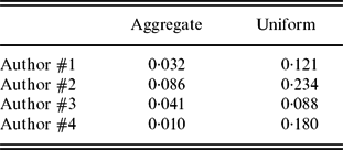
That document sentiment might be useful is intuitive, and part of our reason for reviewing document sentiment analysis techniques in Section 2.2. The result that document-level classifiers did worse than sentence-level ones on different-affect sets of words (as opposed to same-affect ones) went against that intuition, and led to the authorial style idea inspired by the work of Wiebe et al. (Reference Wiebe, Wilson, Bruce, Bell and Martin2004). To check this idea that a particular author's style might be distinguishable (and therefore perhaps useful in detecting this creative choice of same-affect words), we did a quick analysis of the development set. With most of the same-affect instances being negative, we looked at the distribution of negative words as broken down by the 10-point rating scale (from 0.1 to 1.0), for each author. We then compared each distribution against the aggregate distribution for all authors and against a uniform distribution as measured by their Kullback–Leibler divergence (Kullback and Leibler Reference Kullback and Leibler1951); results are in Table 6. Kullback–Leibler divergence gives a value for the difference between two distributions, or rather, the inadequacy of one distribution as a model for another.
Kullback–Leibler divergences for authors vs aggregate and uniform distributions
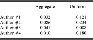
Note that scores for individual authors vary by a factor of 4 (versus uniform) or 8 (versus aggregate). There is no generally agreed interpretation of absolute Kullback–Leibler divergence values, but the point to be drawn here is that some authors are much more different from the typical case in their use of negative words than are others. Also of note is that use of particular near synonyms and other similar linguistic phenomena where language allows a certain amount of choice at a local level is useful in the opposite task: given a document with certain features, identify its author (Koppel, Akiva and Dagan Reference Koppel, Akiva and Dagan2006b). Supporting the idea that author information is useful from a different type of source, author-topic models – topic models of documents, defined via a generative model, that include a model of the author – can display improved predictive power beyond document models of just topic alone (Rosen-Zvi et al. Reference Rosen-Zvi, Griffiths, Steyvers and Smyth2004).
We discuss our models incorporating document sentiment and author information in the next section.
6 Sentiment-derived features with unigrams
6.1 Document sentiment
We constructed two types of models to incorporate document sentiment. The first was just to use the sentiment of each review given in the movie review corpus. This is a gold-standard sentiment, but does not contribute many features. Our second type of model was to use the sentiment of individual words in the document, the sort of feature often used in document sentiment classification; for this, we used scores from MicroWNOP (Cerini et al. Reference Cerini, Compagnoni, Demontis, Formentelli and Gandi2007), a subset of WordNet annotated with polarity information.
MicroWNOP assigns scores to synsets based on their perceived Positive and Negative semantics as judged by human annotators. Cerini et al. (Reference Cerini, Compagnoni, Demontis, Formentelli and Gandi2007) divide the synsets into three groups:
• the Common group, with one Positive and one Negative score per synset (with the pool of five annotators working collaboratively);
• the Group1 group, with three Positive and three Negative scores per synset (three annotators giving individual annotations); and
• the Group2 group, with two Positive and two Negative scores per synset (the remaining two annotators giving individual annotations).
An example entry from Group1 is baseborn, humble and lowly, with all three annotators assigning it 0 for positivity; the first two assigned 0.5 for negativity, and the third 0.25 for negativity. As with SentiWordNet, the entire synset is assigned the score, not any individual words within it.
6.1.1 Gold-standard sentiment
The first set of features, DocSent, is as follows:
• the sentiment of the document in question, as assigned by the rating measurementFootnote 16 of the Scale 1.0 corpus; and
• the sentiment of the target word, as assigned in the annotation (Section 3.2).
6.1.2 Approximate sentiment
This set of features includes the features from Section 6.1.1 and adds features from MicroWNOP. We construct the following definition of a single MicroWNOP Positive score and MicroWNOP Negative score for a word. The MicroWNOP Positive score for a word is the highest single Positive score assigned to a synset containing that word, whether assigned in the Common, Group1 or Group2 categories. The MicroWNOP Negative score is the equivalent value for the negative scores.
We then define four features, intended to be a proxy for the document sentiment:
• the sentiment of the target word, as assigned by annotators in Section 3.2;
• the average of the MicroWNOP Positive scores of all of the words in the document, excepting the target word;
• the average of the MicroWNOP Negative scores of all the words in the document, excepting the target word; and
• the total MicroWNOP Positive scores of all the words in the document, excluding the target, minus the MicroWNOP Negative scores of all the words in the document, excluding the target.
6.2 Author identity
Author identity is also given in Scale 1.0. We thus define AuthorID, four binary features representing each of the four authors in the Scale 1.0 corpus. We use a ‘one-hot’ representation: the single feature corresponding to the particular author is active when it is that author who wrote the review in which the gap occurs, and the other three features inactive.
6.3 Results and discussion
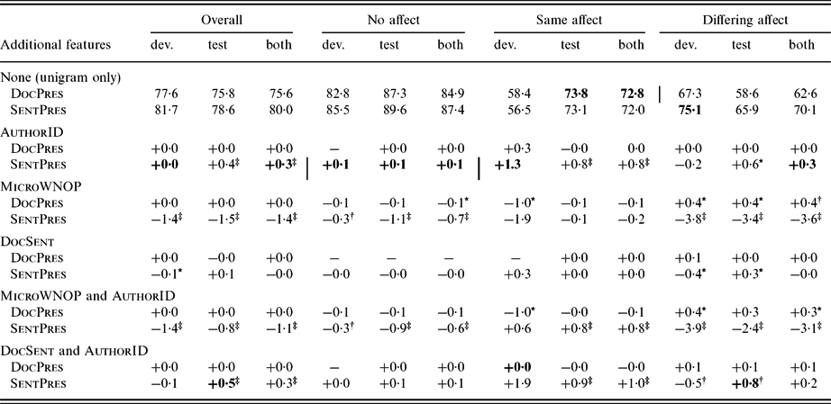
Results comparing various combinations of the above features with unigram features are shown in Table 7 as an accuracy rating and a percentage increase over the unigram baseline. Features were only tested in conjunction with DocPres and SentPres, as the better performing unigram baselines in Section 5.
Performance of SVMs using unigrams with additional features, compared to unigram presence models
Bold values are best performance for that column.
A − means model's choice of word was identical to the unigram presence model, + 0.0 means an increase of < 0.05, − 0.0 means a decrease with absolute value < 0.05.
*Difference from unigram model significant at the p < 0.05 level.
†Difference from unigram model significant at the p < 0.01 level.
‡Difference from unigram model significant at the p < 0.001 leve.
Table 7 shows that for the most part these features have little to no impact on prediction accuracy. However, AuthorID (whether by itself or in conjunction with DocSent) always produces the best results. In three of the cases, it is only by a small margin, with the exception being the case of AuthorID on the sentence frequency classifier. The addition of AuthorID to the sentence presence unigrams, which outperform document presence unigrams on the other word set classes, comes closest to approximating the document presence results on the same affect word sets.
To look further into our intuition that knowledge of the author reflects the linguistic creativity discussed above, we examined the impact of a document frequency (DF) threshold (Yang and Pedersen Reference Yang and Pedersen1997). A major conclusion of Wiebe et al. (Reference Wiebe, Wilson, Bruce, Bell and Martin2004) was that rare events such as hapax legomena contain a lot of information for subjective texts, and so feature selection such as by DF thresholding would be harmful. Therefore, we might expect that DF thresholding would worsen results here if this linguistic creativity is what has led to the same-affect results. For this, we examined the development set (which has similar overall results on the various classifiers). Using DF thresholding values of 2, 4 and 8 caused small decreases (typically around +0.1% at a DF of 8) in the performance of all of the features above. The small magnitude of these suggested that the source of the same-affect results might be elsewhere.
If we consider a practical task, rather than the situation above where we are just investigating the nature of the influence of the author, we would likely not know the author, and have to approximate author identity in order for the method to be effective on unseen text by unknown authors. Given the small magnitude of the improvement, this would likely be overwhelmed by errors in predicting the author, and so not a practical suggestion for such a task. We therefore turn our attention to an alternative way of looking at broader document context.
7 Unigram models accounting for distance
7.1 Distance measure
Our finding in Section 5 that sentence presence features usually outperform document presence features coheres with the finding of Edmonds (Reference Edmonds1997) that a very small window around the data provided better choice accuracy. (Subsequent authors have tended not to evaluate very wide windows in the first place.) Presumably, the noise in the more distant words overwhelms any useful information they convey. However, the finding for the same-affect set that document presence improves performance hints that document-level features can have an impact on the FITB task at least in some cases. This has parallels in work on the behaviour of context with respect to entropy, whose underlying principle as described by Qian and Jaeger (Reference Qian and Jaeger2010) is ‘that distant contextual cues tend to gradually lose their relevance for predicting upcoming linguistic signals’. This idea was first presented in the context of an exploration of the behaviour of entropy by Genzel and Charniak (Reference Genzel and Charniak2002), where they propose the Constant Entropy Rate principle. By conditionally decomposing entropy with respect to local (i.e. sentence-level) and broader context, they empirically demonstrate support – through the consistently observed increase in entropy conditioned on local context throughout texts – for their principle, and conclude that broader context continues to influence later text. They develop this further in Genzel and Charniak (Reference Genzel and Charniak2003), where they find changes in entropy behaviours at paragraph boundaries, suggesting topic or other broader context characteristics are part of the effect. Their principle has subsequently been supported by work in psycholinguistics, such as that of Keller (Reference Keller, Lin and Wu2004), Levy and Jaeger (Reference Levy, Jaeger, Schlkopf, Platt and Hoffman2007), and Gallo, Jaeger and Smyth (Reference Gallo, Jaeger and Smyth2008). Qian and Jaeger (Reference Qian and Jaeger2010) go on to investigate the precise type of relationship of broader context, and find that incorporating linear and sub-linear representations of broader context into entropy models improves the fit of these models of the development of entropy throughout a text.
As noted in Section 5, work in the structurally similar task of word sense disambiguation has generally ignored broader context. Prompted by the results in the previous section and the work on discourse entropy, in this section we describe another model, in which unigram features are weighted by their distance from the gap. Weighting feature values has been explored in a number of machine learning contexts, often drawing on Information Retrieval tools – Paltoglou and Thelwall (Reference Paltoglou and Thelwall2010) is an example, investigating various weighting schemes in the context of document sentiment analysis – but whereas these are typically for whole-document classification and weight feature values identically within a document (e.g. by tf.idf), our weighting scheme is a function of distance.
Rather than using feature value 1 for presence or 0 for absence, as in the unigram models in Section 5, here we weight the presence of a token by its distance from the gap. For example, in the sentence fragment in (7.1) the distance of the token big from the gap is 1, and the distance of economists from the gap is 7.
(10) . . . some economists think it would be a big ________.
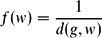
In order that features further away from the gap not be entirely eliminated by their distance from the gap, but that noise not overwhelm the information they bring, we experiment with weighting the distance using the following functions for the feature value f(w) of a token w using distance d(g, w) in number of tokens between w and gap g:
• Inverse linear weighting, InvLinear:
(11)
\begin{equation}
f(w)=\frac{1}{d(g,w)}
\end{equation}
• Inverse square root weighting, InvSquareRoot:
(12)
\begin{equation}
f(w)=\frac{1}{\sqrt{d(g,w)}}
\end{equation}
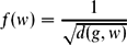
As in Section 5, every token in the document is considered as a feature, except those with total corpus frequency of less than four and the candidates to fill the gap themselves. If a token w is used more than once in a document, the largest value for f(w), ie the smallest d(g, w) for both InvLinear and InvSquareRoot for a given gap g is used.
We test the effectiveness of limiting the features to text surrounding the target word, using the following measures:
• every token in the document;
• every token in the sentence containing the gap and the two surrounding sentences; and
• every token in the sentence containing the gap, only.
We also test the InvSquareRoot unigram model with selected successful additional features from Section 6, giving us the following models:
(1) InvSquareRoot
(2) InvSquareRoot and AuthorID combined
(3) InvSquareRoot and DocSent combined
(4) InvSquareRoot, AuthorID and DocSent combined.
7.2 Results and discussion
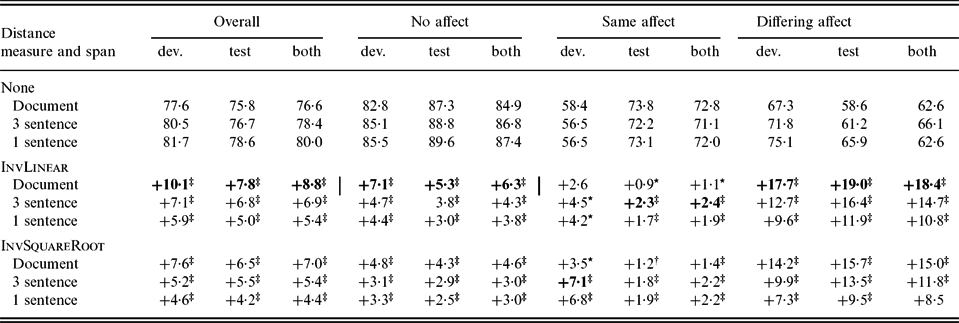
Results are shown in Table 8. We see that weighting the unigrams for their distance from the gap is useful in all cases, giving very large relative improvements over the baseline (in error reduction, up to 48% for differing-affect sets with InvLinear). This general pattern accords with the behaviour of broader context in the entropy work discussed earlier.
Performance of SVMs using distance measures, compared to unigram presence models
Bold values are best performance for that column.
*Difference from non-distance weighted unigram model significant at the p < 0.05 level.
†Difference from non-distance weighted unigram model significant at the p < 0.01 level.
‡Difference from non-distance weighted unigram model significant at the p < 0.001 level.
While this result is to some extent expected – words closer to the gap have a higher weight, and thus the most predictive power over the word filling the gap – the most interesting result is that a wider context than sentence level remains useful. The result even extends beyond the three-sentence level to the entire document, so that in at least some cases words quite far from the gap indeed are affecting the choice of near synonym: drilling down into the data for examples, the improvement for the set ludicrous, senseless, foolish, . . . with document-level context is +11.2% over the baseline versus +6.6% for three-sentence context (both InvSquareRoot); the improvement for aloof, detached, reserved is +17.2% for document-level context versus +13.1% for three-sentence context (again InvSquareRoot). As with the unigram results from Section 5, this supports our hypothesis that features of the entire document influence the choice of near synonym, even though document-level features do not appear to have been well captured by our choice of features in Section 6.
One possible reason for this is connected to empirical work by, for example, Bieler, Dipper and Stede (Reference Bieler, Dipper and Stede2007), which has found that movie (and other similar) reviews have a semi-conventionalised structure: there are distinguishable ‘functional zones’, with more objective descriptive material tending to cluster together separately from more subjective commentary. Perhaps the weighting is implicitly giving more prominence to the context in the same functional zone.Footnote 17
Same-affect near synonyms also respond better to a different weighting function, InvSquareRoot rather than InvLinear. InvSquareRoot discounts the distance between a word and the gap less heavily than InvLinear does, especially, relatively speaking, at more extreme distances. This further demonstrates that more distant words are having an effect: some discounting is evidently required since InvSquareRoot outperforms no weighting, but there is an extent past which the discounting appears to under-weight features when the entire document is required as context.
As for the general utility of the weighting functions, having no weighting function results in the document context performing 3.4% worse than the single sentence context: this is consistent with the discussion in Section 5.2 on previous and related results, where the document context just adds noise. Weighting functions boost the results for both the single sentence context and the document context; for the no-affect and differing-affect sets and the InvLinear function, this is to the same (highest performing) level. The weighting function thus seems like a good way of ignoring noise, although it does not entirely compensate for extending the context beyond what is necessary.
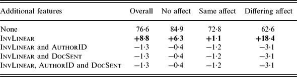
Results for the combination of the InvLinear weighting with other features is given in Table 9. In all of these cases, adding the features was harmful. Distance weighting thus appears to capture document tone better than the explicit features of author ID or document sentiment.
Performance of SVMs using InvLinear with additional features, compared to the DocPres unigram model
Bold values are the best performance for that column.
We have thus further confirmed our result that in many cases, a very wide context is useful, and we have gone some way to narrowing down exactly how to balance providing this context with weighting appropriately for noise. Further work is needed to determine how to distinguish contexts where words very distant from the gap should be included with appropriate weights, as in our same-affect set, and where they should be excluded entirely, or weighted even lower than InvLinear.
7.3 Examples of the best performing sets
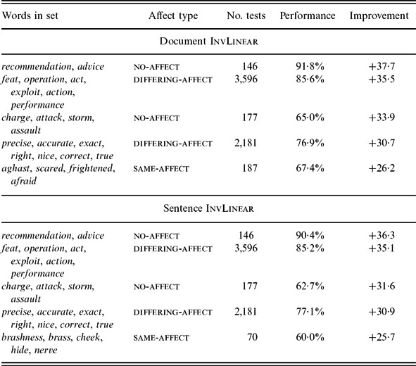
As an illustration, the best performing five near synonym sets relative to improvement over the baseline – that is, those where broader context and distance-weighting were particularly useful, which would not be captured by more typical small context window sizes – are shown in Table 10 for both document InvLinear and sentence InvLinear. For both techniques, the largest improvements are in fact delivered over the full range of set types, including no affect. The only difference is the appearance of different same-affect sets in the top five: aghast etc. in the document list and brashness etc. in the sentence list, with each being seventh in the other list.
Best performing five sets for each of document and sentence InvLinear, relative to baseline performance
8 Conclusion
In this paper, we have applied a previously untried supervised approach to the problem of choosing the right near synonym to fill a lexical gap. Our main conclusions from doing this are as follows. First, as per Pang et al. (Reference Pang, Lee and Vaithyanathan2002) with document sentiment classification, unigrams alone do well, with presence outperforming frequency, and with immediate-context (sentence) models generally outperforming wider-context (document) models. Second, that once appropriate weighting of distance features are incorporated, the technique performs near-synonym choice notably better with document rather than sentence features; this may be a consequence of a particular ‘tone’ suffusing the document. Third, adding in one possible factor related to this tone, knowledge of the author of the text, gives slightly better results overall, in particular improving sentence presence results for same-affect near synonyms; this author effect was not expected at the start of the work. Fourth, the most significant improvement came from incorporating document-level information using a weighting scheme, which in fact improved over the earlier best sentence-level models, and which in its description of the effect of broader context mirrors work on the effect of the Constant Entropy Rate principle. This is true for all near-synonym sets, including the non-affect ones.
There are a number of directions for future work. In terms of the specific task tackled in this article, there could be more investigation into how precisely this author and distance information are causing the improvement discovered, and whether more sophisticated models could capture this. In terms of alternative approaches, dependency relations could be promising, either in terms of structured language models (Xu, Chelba and Jelinek Reference Xu, Chelba and Jelinek2002) or as additional features in the supervised model (Özgür and Güngör Reference Özgür and Güngör2010). In terms of applications, the techniques in the article could be applied to the sentiment-directed text rewriting noted at the start of the article described in Inkpen et al. 2006, or the intelligent thesaurus of Inkpen (Reference Inkpen2007a). In both of these applications, as well as the FITB task of this article, it would be useful to devise and carry out human evaluations – for FITB, for example, alternatives besides the original choice might be acceptable – which could feasibly be done with the availability of services like Mechanical Turk.
Appendix A: Word sets with sentiment differences
These are the 47 word sets drawn from Use the Right Word (Hayakawa Reference Hayakawa1968) as described in Section 3.2. The annotation Positive, Neutral or Negative is given for each word; sets are annotated as None (no affect), Same (same affect) or Differing (differing affect). The number of instances of each set is given under Size.
Appendix B: Language models
Here we detail the implementation of our language model prediction system using the Web1T data in order to test whether our methods out-perform language models. We consider predicting a word choice as estimating the most probable 3-gram. In example 1 we would be trying to estimate the most probable of the following 3-grams:
(13) a big error
(14) a big mistake
(15) a big oversight
We would then choose from among error, mistake and oversight by choosing the word contained in the most probable 3-gram.
As is common in language models, we backoff to 2-grams and 1-grams where necessary. We draw our discussion that follows from the original paper of Katz (Reference Katz1987), the more detailed explication of Gale and Sampson (Reference Gale and Sampson1995), and the overview of Jurafsky and Martin (Reference Jurafsky and Martin2009). In general, backoff models look like this:
• The count of n-gram w 1, . . ., wn in the training data is denoted by
(16)
\begin{equation}
C(w_{1},\ldots, w_{n})
\end{equation}
• The smoothed count C* of n-gram w 1, . . ., wn is given by the specific smoothing algorithm.
• The adjusted probability P* of n-gram w 1, . . ., wn is given by
(17)
\begin{equation}
P^*(w_{n}|w_{1},\ldots, w_{n-1})= \frac{C^*(w_{1},\ldots, w_{n})}{C(w_{1},\ldots, w_{n-1})}
\end{equation}
• If a count for w 1, . . ., wn is unavailable, P(wn|w 1, . . ., w n−1) is estimated using the counts for n-gram w 2, . . ., wn using a backoff model, where α is a the proportion of the probability space reserved for unseen events:
(18)
\begin{equation}
P(w_{n}|w_{1},\ldots, w_{n-1})=\alpha (w_{1},\ldots, w_{n-1})P(w_{n}|w_{2},\ldots, w_{n-1})
\end{equation}



In the smoothing and backoff implementation of Katz (Reference Katz1987) the specifics of these functions are:
• The number of n-grams with count c in the training data is denoted by
(19)
\begin{equation}
r(c)
\end{equation}
• The adjusted count C* of an n-gram w 1, . . ., wn is smoothed by the Good-Turing estimation (Good Reference Good1953) and is given by
(20)
\begin{equation}
C^*(w_{1},\ldots, w_{n})=\frac{(C(w_{1},\ldots, w_{n}) + 1)\cdot r(C(w_{1},\ldots, w_{n}) + 1)}{r(C(w_{1},\ldots, w_{n}))}
\end{equation}
• The proportion α of the total probability mass allocated to unseen words wn following w 1, . . ., w n−1 is given by
(21)where the function β is given by
\begin{equation}
\alpha (w_{1},\ldots, w_{n-1}) = \frac{\beta (w_{1},\ldots, w_{n-1})}{\sum _{w_{n}:C(w_{2},\ldots, w_{n})>0}P^*(w_{n}|w_{2},\ldots, w_{n-1})}
\end{equation}
(22)
\begin{equation}
\beta (w_{1},\ldots, w_{n-1})=1-\sum _{w_{n}:C(w_{1},\ldots, w_{n})>0} P^*(w_{n}|w_{1},\ldots, w_{n-1})
\end{equation}




In a typical language model implementation, at some sufficiently large value of r the probability of n-gram w 1, . . ., wn, P(wn|w 1, . . ., w n−1) would be estimated using a maximum likelihood estimate instead, given in (23), as in for example Gale and Sampson (Reference Gale and Sampson1995):
 \begin{equation}
P(w_{n}|w_{1},\ldots, w_{n-1})= \frac{C(w_{1},\ldots, w_{n})}{C(w_{1},\ldots, w_{n-1})}
\end{equation}
Given that we are using Web1T for our values of C(w 1, . . ., wn), and Web1T does not provide counts for r < 40 for bi- to 5-grams and for r < 200 for we use (23) rather than (17). There are several reasons for this. The first is that the standard methods for determining the value of this cut-off would usually be applied on the tail end of the data, precisely what has been removed from Web1T.
The second is that even for fairly low values of r available in Web1T, ie r ≈ 40, C*(w 1, . . ., wn) > C(w 1, . . ., wn) when using (20) to compute C*. This results in periodic cases where β < 0 in (22).
Given this, we also estimate α differently from (21). The Web1T corpus does not include n-grams for n ⩾ 2 with counts of less than 40 (or unigrams with counts of less than 200). We therefore estimate the probability mass allocated to unseen n-grams by the proportion of the count of an n-gram w 1, . . ., wn unaccounted for by known n + 1-grams w 1, . . ., w n + 1. To give an example of how this is done, let us assume that bigram mistakes are has a Web1T count of 300, and the only trigrams beginning with mistakes are are mistakes are bad and mistakes are good, with counts of seventy-five each. We then have 150 unseen tokens following mistakes are and thus the value of α is 0.5.
This can be formally expressed as
 \begin{equation}
\alpha (w_{1},\ldots, w_{n-1}) = \frac{\sum _{w_{n}:C(w_{1},\ldots, w_{n})>0}C(w_{1},\ldots, w_{n})}{C(w_{1},\ldots, w_{n-1})}
\end{equation}