



1. Introduction
Morphological patterns on the interface in multi-phase flows are ubiquitous in nature, such as the ripples on the surface of icicles (Ogawa & Furukawa Reference Ogawa and Furukawa2002), wave-like structures on glaciers (Camporeale & Ridolfi Reference Camporeale and Ridolfi2012b ), crenulations on stalactites (Camporeale & Ridolfi Reference Camporeale and Ridolfi2012a ), dimples over a bed of sand below shallow wavy water (Lundbek Hansen et al. Reference Lundbek Hansen, van Hecke, Haaning, Ellegaard, Haste Andersen, Bohr and Sams2001; Charru, Andreotti & Claudin Reference Charru, Andreotti and Claudin2013), scallops on the side of icebergs (Bushuk et al. Reference Bushuk, Holland, Stanton, Stern and Gray2019), and patterns on lava flows (McDonald et al. Reference McDonald, Méndez Harper, Ojha, Corlies, Dufek, Ewing and Kerber2022). Among them, the ripples formed on the ice surface, e.g. patterns on icicles, glaciers (see figure 1 a), icy rivers and frozen lakes (see figure 1 b), are related to perturbation growth in phase-change processes. These patterns change the surface roughness, which has been reported to be in strong correlation with the melt rates, e.g. in ice shelves (Watkins, Bassis & Thouless Reference Watkins, Bassis and Thouless2021). Investigating these pattern formations is critical to unveil the underpinning mechanism, and is of tremendous interest in developing anti-icing and de-icing devices for applications (Zhang et al. Reference Zhang, Shahmardi, Choi, Tammisola, Brandt and Mao2022a ).
Efforts have been devoted to investigating the structure of ice, as well as its growth mechanisms (Murata, Nagashima & Sazaki Reference Murata, Nagashima and Sazaki2019; Wang et al. Reference Wang, Calzavarini, Sun and Toschi2021; Grivet et al. Reference Grivet, Monier, Huerre, Josserand and Séon2022). It has been well demonstrated that the growth of an icicle is complicated and sensitive to atmospheric conditions and the water flux (Makkonen Reference Makkonen1988), highlighting the importance of the water and air dynamics in the consolidation process. Zwally et al. (Reference Zwally, Giovinetto, Li, Cornejo, Beckley, Brenner, Saba and Yi2005), Rignot & Kanagaratnam (Reference Rignot and Kanagaratnam2006) and Kaser et al. (Reference Kaser, Cogley, Dyurgerov, Meier and Ohmura2006) studied the evolution of the glaciers in Greenland and the Antarctic, and reported that they can be recognised as structures of ice surrounded by water films since the ice is exposed to meltwater (Camporeale & Ridolfi Reference Camporeale and Ridolfi2012b ), indicating the presence of a three-phase system with water sandwiched by ice and air (see figure 1 c). The evolution of ice on rivers, lakes and ponds has also been studied in previous works (Leppäranta Reference Leppäranta2010; Popović et al. Reference Popović, Cael, Silber and Abbot2018; Blackburn & She Reference Blackburn and She2019).
Examples of ice patterns. (a) Ice ripples on the surface of the Ciardoney glacier (North Italy, 45
 $^\circ$
31
 $'$
N, 7
 $^\circ$
23
 $'$
E) (Camporeale & Ridolfi Reference Camporeale and Ridolfi2012b
). (b) An example of ice ripples on a lake (see the original figure on the website http://lakeice.squarespace.com/ice-ripples/). (c) Schematic view of patterns in ice–water–air flow.

Despite these quantitative studies on the basic structures and the growth of ice, not much attention has been focused on the mechanism of the ripple formation on the ice surfaces. An axisymmetry-breaking instability in the natural convection of water within a vertical cylinder was studied numerically and experimentally. The study showed that a cold metallic surface at the top of the cylinder froze the water, and the ice front grew downwards, exhibiting high-azimuthal-wavenumber patterns in the ice–water flow (Gelfgat et al. Reference Gelfgat, Bar-Yoseph, Solan and Kowalewski1999). A theoretical model based on hydrodynamic stability was proposed to attribute the patterns on the icicles to the growth of infinitesimal perturbations, and the wavelength of the ripples was found to be approximately 1 cm (Ogawa & Furukawa Reference Ogawa and Furukawa2002). Subsequently, linear stability analysis was carried out to interpret icicle ripples, and the influence of ambient air and water on the growth of the ice–water interface disturbance was modelled separately (Ueno Reference Ueno2003, Reference Ueno2004, Reference Ueno2007; Ueno & Farzaneh Reference Ueno and Farzaneh2011). These theoretical and numerical results were validated by comparing the wavelengths against experimental ones (Ueno et al. Reference Ueno, Farzaneh, Yamaguchi and Tsuji2009). However, there is a lack of the influence of the ice layer and water layer thicknesses on the formation of patterns, although it is generally known that different thicknesses lead to distinct ripples in nature (see figure 1 b).
Compared with the limited research on the ripples of icicles, studies on the mechanism of ice ripple formation on glaciers and lakes, where the gravity is not parallel to the interface as in the icicle scenarios, and different mechanisms can be expected, are even rarer. Among them, a mathematical model based on the well-known Orr–Sommerfeld equations was developed by treating the problem as the morphological instability of a melting–freezing interface bounding a free-surface laminar flow (Camporeale & Ridolfi Reference Camporeale and Ridolfi2012b ). However, the role of the air dynamics was not accounted for, only ice and water were considered in this model, and the detailed distribution of perturbations, which is demonstrated to be focused on both the ice–water and water–air interfaces in this paper, was absent.
Another potential theory to explain the mechanism of ripple formation on a horizontal ice surface is the Rayleigh–Taylor (R–T) instability, as the heavier phase (water) is placed above the lighter one (ice) and is accelerated by gravity (see figure 1 c). The R–T instability in two-layer flows has been studied extensively since the pioneering work of Rayleigh (1882) and Taylor (Reference Taylor1950). However, studies on R–T instability in three-layer or multi-layer flows are comparatively limited. Mikaelian (Reference Mikaelian1982) proposed a linear theory to investigate R–T instability at the interfaces of multiple stratified fluids with arbitrary density profiles, assuming that the flows are incompressible and inviscid. Parhi & Nath (Reference Parhi and Nath1991) developed a formulation for R–T instability in three-layer incompressible and viscous flows. Jacobs & Dalziel (Reference Jacobs and Dalziel2005) conducted experimental investigations on R–T instability in three-layer fluids, with one unstable and one stable interface, and examined the influence of the density difference between the top and bottom layers. More recently, Adkins et al. (Reference Adkins, Shelton, Renoult, Carles and Rosenblatt2017) used a fluid magnetic levitation technique to experimentally study R–T instability in three-layer flows with a low–high–low density distribution. Their results showed that the growth rate decreases as the height of the middle layer increases. Following this, the influences of cylindrical geometry (Guo et al. Reference Guo, Wang, Ye, Wu and Zhang2017), non-uniform velocity shear (Matsuoka Reference Matsuoka2020), strong isothermal stratification (Aslangil & Wong Reference Aslangil and Wong2023) and nonlinear dynamics (Sengupta, Ulloa & Joshi Reference Sengupta, Ulloa and Joshi2023) on R–T instability in three-layer flows have been explored successively. However, limited efforts have been devoted to the effects of the thicknesses of different layers, which are critical to the icing problem studied in this work. Furthermore, existing research on the R–T instability is mainly on the interface of fluid phases, and there has been no study on the role of the R–T instability on the ripple formation around the ice surface, where heavier fluid is above lighter solid.
The purpose of this work is to investigate the mechanisms of the morphological patterns on the ice surface of glaciers and lakes with a shallow film of air-surrounded water flows, as well as the influence of the ice and water thicknesses. To study the icing process and ripple formation in such a three-phase flow, how to capture the interfaces between different phases is one of the key issues. In the mid-20th century, the idea of a non-zero thickness interface was developed, and the phase-field method was proposed (Cahn & Hilliard Reference Cahn and Hilliard1958). This method circumvents the imposition of boundary conditions on the interface by introducing additional variables that are continuous in the domain so that the physical variables do not exhibit mutations at the interface (Mirjalili, Ivey & Mani Reference Mirjalili, Ivey and Mani2019). Taking this advantage, this method was then applied in the simulation of multi-phase flows such as solidification (Sabouri-Ghomi, Provatas & Grant Reference Sabouri-Ghomi, Provatas and Grant2001), melting (Weady et al. Reference Weady, Tong, Zidovska and Ristroph2022), boiling (Badillo Reference Badillo2012) and sublimation (Reitzle et al. Reference Reitzle, Ruberto, Stierle, Gross, Janzen and Weigand2019), to name a few. In spite of these successful applications, there is a lack of modelling of ice ripples based on the phase-field method. Therefore, we establish a theoretical model for ice–water–air flows with phase change. The linear stability analysis is then carried out to study the morphological instability of the flows and subsequently examine the natural ice pattern growth. We find that the patterns on the ice surfaces are formed by the growth of the perturbations, which are generated on the ice–water interface, owing to an instability analogous to the gravity-driven R–T form generally found on the interface of two fluids, and propagate to the water–air interface. We note that the linear stability theory applied in this work predicts the most unstable wavelength of interface instabilities marking the formation of ripples, whilst the saturated magnitude of ripples and three-dimensional developments requiring nonlinear calculations are out of the scope of this work.
2. Governing equations
2.1. Phase-field model for three-phase flows
As shown in figures 1(a) and 1(b), a thin layer of meltwater is commonly anticipated to be present above the ice layer. The water, surrounded by the ambient air, has complex interactions with ice and air, which are characterised by the ice–water and water–air interfaces, respectively. For such a configuration, a two-dimensional study, as depicted in figure 1(c), is sufficient. The
 $x$
direction is parallel to the unperturbed interface, and
 $y$
is normal to it. Two phase-field order parameters,
 $\phi$
and
 $c$
, are employed to mark the three phases and subsequently the interfaces:
 $\phi \in [-1, 1]$
is used to distinguish air (
 $\phi =-1$
) from water (
 $\phi =1$
), while
 $c \in [-1, 0]$
is employed to separate water (
 $c=0$
) from ice (
 $c=-1$
). The volume fractions of the air, water and ice phases in the proposed model are obtained as
 $\beta _g=(1-\phi )/2,\ \beta _l=(1+\phi )(1+c)/2,\ \beta _s=(1+\phi )(-c)/2$
, where
 $\beta _g+\beta _l+\beta _s=1$
is always true in the whole domain. Based on the volume fractions of the phases, density, viscosity, thermal conductivity and specific heat capacity are obtained by linear interpolations:
 \begin{equation} \begin{aligned} \rho (c,\phi )&=\beta _g \rho _g + \beta _l \rho _l + \beta _s \rho _s,\\[2pt] \mu (c,\phi )&=\beta _g \mu _g + \beta _l \mu _l + \beta _s \mu _s, \\[2pt] \kappa (c,\phi )&=\beta _g \kappa _g + \beta _l \kappa _l + \beta _s \kappa _s,\\[2pt] c_p(c,\phi )&=\beta _g c_{pg} + \beta _l c_{pl} + \beta _s c_{ps}, \end{aligned} \end{equation}
where
 $\rho$
is the density,
 $\mu$
is the viscosity,
 $\kappa$
is the thermal conductivity,
 $c_p$
is the specific heat capacity, and the subscripts
 $g$
,
 $l$
and
 $s$
represent pure air, pure water and pure ice, respectively.
The Allen–Cahn equation (Allen & Cahn Reference Allen and Cahn1979) is used to model the phase change from water to ice:
 \begin{equation} \frac {\partial c }{\partial t } + \boldsymbol{\nabla} \boldsymbol{\cdot} ({\boldsymbol{u}} c )=M_c\left[6 \sigma _c\xi _c\,\boldsymbol{\nabla} ^{2}c-\frac {\partial f(c)}{\partial c}\right], \end{equation}
where
 $\boldsymbol u$
denotes the velocity vector,
 $t$
is time,
 $M_c$
is the phenomenological mobility, whose larger value speeds up the phase-changing process (Zhang et al. Reference Zhang, Shahmardi, Choi, Tammisola, Brandt and Mao2022b
),
 $\sigma _c$
and
 $\xi _c$
denote the surface tension and the thickness coefficient of the ice–water interface, respectively. Here,
 $f(c)=3({\sigma _c}/{\xi _c})\,g(c)+L({T_M-T})\,h(c)/{T_M}$
is the free energy density, where
 $g(c)=(c+1)^2c^2$
,
 $h'(c)=30\,g(c)$
,
 $L$
is the latent heat of fusion per unit volume,
 $T$
is the temperature, and
 $T_M$
is the melting point of ice (Boettinger et al. Reference Boettinger, Warren, Beckermann and Karma2002; Zhang et al. Reference Zhang, Shahmardi, Choi, Tammisola, Brandt and Mao2022b
).
The Cahn–Hilliard equation (Cahn & Hilliard Reference Cahn and Hilliard1958) is employed to model the evolution of the interface between water and air:
 \begin{equation} \frac {\partial \phi }{\partial t} + \boldsymbol u \boldsymbol{\cdot} \boldsymbol{\nabla} \phi = M_\phi\, \boldsymbol{\nabla} ^{2} \mu _{\phi }, \end{equation}
where
 $M_\phi$
is the phenomenological mobility, and
 $\mu _\phi$
is the chemical potential obtained from (Boettinger et al. Reference Boettinger, Warren, Beckermann and Karma2002; Zhang et al. Reference Zhang, Shahmardi, Choi, Tammisola, Brandt and Mao2022b
; Wang et al. Reference Wang, Zhang, Mao, Choi and Li2024)
 \begin{equation} \mu _\phi = -\frac {3\sigma _\phi }{2\sqrt 2}\left [ \xi _\phi\, \boldsymbol{\nabla} ^{2}\phi -\frac {1}{\xi _\phi }(\phi ^{3}-\phi )\right ], \end{equation}
where
 $\sigma _\phi$
and
 $\xi _\phi$
denote the surface tension and the thickness coefficient of the water–air interface, respectively.
The continuity, momentum and energy equations for the multi-phase flow are
 \begin{align}&\qquad\qquad\qquad\qquad\quad \frac {\partial \rho }{\partial t}+\boldsymbol{\nabla} \boldsymbol{\cdot} (\rho \boldsymbol u) =0, \end{align}
 \begin{align}&\qquad\quad\,\, \frac {\partial (\rho \boldsymbol u)}{\partial t}+\boldsymbol{\nabla} \boldsymbol{\cdot} (\rho \boldsymbol u \otimes \boldsymbol u)=-\boldsymbol{\nabla} p + \boldsymbol{\nabla} \boldsymbol{\cdot} \boldsymbol \tau + \boldsymbol{F}_b, \end{align}
 \begin{align}& \frac {\partial (\rho c_p T)}{\partial t}+\boldsymbol{\nabla} \boldsymbol{\cdot} (\rho c_p T \boldsymbol u) =\frac {\partial \beta _s}{\partial t}L+\boldsymbol{\nabla} \boldsymbol{\cdot} (\kappa \boldsymbol{\nabla} T ) +\Phi + \boldsymbol u \boldsymbol{\cdot} \boldsymbol{F}_b, \end{align}
where
 $\otimes$
represents the outer product,
 $p$
denotes pressure,
 $\boldsymbol \tau =-2/3\mu \boldsymbol{\nabla} \boldsymbol{\cdot} \boldsymbol u\boldsymbol I+\mu [\boldsymbol{\nabla} \boldsymbol u+(\boldsymbol{\nabla} \boldsymbol u)^{\rm T}]+\boldsymbol \tau _e$
is the total stress tensor, with
 $\boldsymbol I$
the unit diagonal tensor, superscript
 ${\rm T}$
indicating the transpose of a matrix, and
 $\boldsymbol \tau _e=-({3}/{2\sqrt {2}})\sigma _c \xi _c\,\boldsymbol{\nabla} c \otimes \boldsymbol{\nabla} c -({3}/{2\sqrt {2}})\sigma _{\phi } \xi _\phi\, \boldsymbol{\nabla} \phi \otimes \boldsymbol{\nabla} \phi$
being the extra elastic stress induced by the interfacial surface tension (Liu & Shen Reference Liu and Shen2003; Shen Reference Shen2011). Also,
 $\boldsymbol{F}_b=\rho \boldsymbol{g}$
is the body force, with
 $\boldsymbol{g}$
denoting the gravitational acceleration, and
 $\Phi$
is the viscous dissipation rate. The first term on the right-hand side of the energy equation (2.7) describes the latent heat due to phase change in the icing process. Note that although the fluid flow (water and air) is considered incompressible in this work, the use of a compressible form of the equations is more rigorous in phase-field models, as properties such as density and viscosity vary continuously from phase to phase around the interfaces (see (2.1)) (Kim Reference Kim2012).
2.2. Linear stability equations
To study the dynamics of small perturbations, whose growth leads to the development of patterns on the ice surface, the flow field is decomposed into a base flow and a small perturbation:
 \begin{eqnarray} \boldsymbol q =\boldsymbol q_0 +\boldsymbol q', \end{eqnarray}
where
 $\boldsymbol q = [\boldsymbol u, p, c, \phi ,\mu _\phi , T]^{\rm T}$
denotes the flow variables,
 $\boldsymbol q_0 = [\boldsymbol u_0, p_0, c_0, \phi _0,\mu _{\phi 0}, T_0]^{\rm T}$
is the steady base flow satisfying the governing equations (2.2)–(2.7) and varying in the
 $y$
direction only, and
 $\boldsymbol q' = [\boldsymbol u', p', c', \phi ',\mu _\phi ', T']^{\rm T}$
is the perturbation that can be further decomposed in
 $x$
and
 $t$
, and each term reads
 \begin{eqnarray} \boldsymbol q'(x,y,t)={\hat {\boldsymbol q}}(y) \textrm { exp}(\textrm{i}\alpha x -\textrm{i}\omega t), \end{eqnarray}
where
 $\hat {\boldsymbol q}$
is the amplitude of the perturbation, and
 $\alpha$
denotes the wavenumber. Here,
 $\omega =\omega _r+i\omega _i$
is a complex value (with
 $\textrm{i}$
the imaginary unit), with
 $\omega _r$
and
 $\omega _i$
representing the angular frequency and the growth rate of the perturbation, respectively. By substituting (2.8) into (2.2)–(2.7), subtracting the base flow terms, and neglecting the nonlinear terms of perturbations, the linear stability equations for the perturbations can be obtained:
 \begin{eqnarray} \boldsymbol{\Gamma } \frac {\partial \boldsymbol q'}{\partial t} +\boldsymbol{H}_x\frac {\partial \boldsymbol q'}{\partial x} +\boldsymbol{H}_y \frac {\partial \boldsymbol q'}{\partial y}+\boldsymbol{H} \boldsymbol q'+\boldsymbol{H}_{xx} \frac {\partial ^2 \boldsymbol q'}{\partial x^2} +\boldsymbol{H}_{yy} \frac {\partial ^2 \boldsymbol q'}{\partial y^2}+\boldsymbol{H}_{xy} \frac {\partial ^2 \boldsymbol q'}{\partial x\, \partial y}=0,\ \ \ \ \ \end{eqnarray}
where matrices
 $\boldsymbol{\Gamma }$
,
 $\boldsymbol{H}_x$
,
 $\boldsymbol{H}_y$
,
 $\boldsymbol{H}$
,
 $\boldsymbol{H}_{xx}$
,
 $\boldsymbol{H}_{yy}$
and
 $\boldsymbol{H}_{xy}$
are functions of the base flow quantities (see Appendix A for details).
The boundary conditions of the perturbations on the lower boundary (assumed as pure ice) are
 \begin{equation} \boldsymbol u'=0,\quad \frac {\partial p'}{\partial y}=0,\quad c'=0,\quad \phi '=0,\quad \mu^{\prime}_{\phi }=0,\quad T'=0, \end{equation}
where
 $\boldsymbol u'=0$
ensures a no-slip condition, while
 ${\partial p'}/{\partial y}=0$
maintains pressure continuity across the solid boundary. Other perturbations are set to zero, assuming no fluctuations at the ice boundary.
The boundary conditions of the perturbations on the upper boundary (assumed as pure air) are
 \begin{equation} \frac {\partial \boldsymbol u'}{\partial y}=0,\quad p'=0,\quad c'=0,\quad \phi '=0,\quad \mu ^{\prime}_{\phi }=0,\quad T'=0, \end{equation}
where
 ${\partial \boldsymbol u'}/{\partial y}=0$
represents a stress-free condition, and
 $p'=0$
reflects the constant atmospheric pressure. Other perturbations are set to zero.
Substituting (2.9) into (2.10) results in
 \begin{equation} (-i\omega \boldsymbol{\Gamma } +i\alpha \boldsymbol{H}_x +\boldsymbol{H}_y\textrm{D} +\boldsymbol{H} -\alpha ^2\boldsymbol{H}_{xx} +\boldsymbol{H}_{yy}\textrm{D}^2 +i\alpha \boldsymbol{H}_{xy} \textrm{D} )\hat {\boldsymbol q} =0, \end{equation}
where
 ${\rm D}={\rm d}/{\rm d}y$
represents the derivative with respect to
 $y$
. Equation (2.13) is solved as an eigenvalue problem:
 \begin{equation} \boldsymbol{\Lambda } \hat {\boldsymbol q}=\omega \boldsymbol{\Gamma } \hat {\boldsymbol q}, \end{equation}
where
 $\boldsymbol{\Lambda } = \alpha \boldsymbol{H}_x -i\boldsymbol{H}_yD -i\boldsymbol{H} +i\alpha ^2\boldsymbol{H}_{xx}-i\boldsymbol{H}_{yy}D^2+\alpha \boldsymbol{H}_{xy} D$
.
In this paper, the temporal problem is considered, with wavenumber
 $\alpha$
prescribed and
 $\omega$
solved as the eigenvalues. The eigenvalue with the largest imaginary part, denoted as
 $\omega _i^{max}$
, which is the growth rate of the most unstable perturbation, will be the focal of the following discussions.
A second-order finite difference method is applied, and the domain is divided equally into
 $N$
grids, allowing (2.14) to be solved numerically as a discretised generalised eigenvalue problem using the QR algorithm in MATLAB.
3. Base flow
For the configuration shown in figure 1, to ensure the coexistence of ice and water, the temperature of the base flow throughout the entire field is uniformly set to
 $273.15\ \textrm {K}$
. It suffices here to focus on cases with zero base flow velocity, corresponding to a still lake or glacier. In this scenario, the horizontal plane perpendicular to the
 $y$
direction is isotropic, and the system exhibits no preferred instability direction on that plane, leading to an essentially two-dimensional formula of the instability. Therefore, as shown in (2.9), two-dimensional instabilities are considered in our work.
The lower boundary is set as pure ice (
 $c_0=-1,\ \phi _0=1$
), and the upper boundary is treated as pure air (
 $c_0=0,\ \phi _0=-1$
). The boundary conditions of the base flow on the lower boundary are
 \begin{equation} \boldsymbol u_0=0,\quad \frac {\partial p_0}{\partial y}=0,\quad c_0=-1,\quad \phi _0=1,\quad \mu _{\phi 0}=0,\quad T_0=T_M, \end{equation}
and those on the upper surface are
 \begin{equation} \frac {\partial \boldsymbol u_0}{\partial y}=0,\quad p_0=p_{a},\quad c_0=0,\quad \phi _0=-1,\quad \mu _{\phi 0}=0,\quad T_0=T_M, \end{equation}
where
 $p_{a}=101\,325\ \textrm {Pa}$
is the environment pressure, and
 $T_M=273.15 \textrm { K}$
represents the melting point of ice.
The values for the material properties of pure ice, water and air, and the other physical parameters, are shown in table 1 and table 2, respectively (Zhang et al. Reference Zhang, Shahmardi, Choi, Tammisola, Brandt and Mao2022b
). Note that the surface tension at the ice–water interface (
 $\sigma _c$
) is set to
 $3.17 \times 10^{-2}\ \textrm {N m}^{-1}$
according to an experimental study (Hillig Reference Hillig1998).
Properties of air, water and ice.

Values of physical parameters.

Here we give an example of the motionless base flow. The steady solutions of the Allen–Cahn and Cahn–Hilliard equations (see (2.2) and (2.3)) are in the form of hyperbolic tangent type functions (Dadvand et al. Reference Dadvand, Bagheri, Samkhaniani, Marschall and Wörner2021):
 \begin{align}& c_0(y)=-\frac {1}{2}+\frac {1}{2}\tanh\left(\frac {y-H_1}{2\xi _c}\right), \end{align}
 \begin{align}&\quad \phi _0(y)=-\tanh\left(\frac {y-H_2}{\sqrt {2}\,\xi _{\phi }}\right), \end{align}
where
 $H_1$
and
 $H_2$
are arbitrary constants, whose variation produces a collection of solutions for
 $c_0$
and
 $\phi _0$
denoting the positions of ice–water and water–air interfaces. Figure 2 exhibits an example of the solutions for
 $c_0$
and
 $\phi _0$
, where the domain is divided into five regions (ice layer, ice–water interface, water layer, water–air interface, and air layer) along the
 $y$
direction by these order parameters. The other properties of the base flow, i.e.
 $\gamma _0 = (\rho _0, \mu _0, \kappa _0, c_{p0})$
, are calculated by linear interpolation:
 $\gamma _0 =\beta _{g0} \gamma _g + \beta _{l0} \gamma _l + \beta _{s0} \gamma _s$
, where the volume fractions
 $\beta _{g0},\beta _{l0}, \beta _{s0}$
are obtained from
 $c_0$
and
 $\phi _0$
(see (2.1)).
A distribution of phase-field order parameters
 $c_0$
and
 $\phi _0$
in the base flow.

4. Sensitivity studies
We first conduct a grid independence study. Figure 3 shows the dispersion relation of the growth rate
 $\omega ^{max}_i$
with wavenumber
 $\alpha$
at different numbers of grid points
 $N$
, with both the ice layer thickness
 $l_{ice}$
and the water layer thickness
 $l_{water}$
set to 2 mm. The results demonstrate that
 $N=600$
is sufficient for convergence (with relative errors less than 1
 $\%$
compared to
 $N=800$
), and this value is therefore adopted in this work.
Dispersion relation of growth rate
 $\omega ^{max}_i$
with wavenumber
 $\alpha$
for different grid numbers with
 $l_{ice}=l_{water}=2$
mm.

We then conduct sensitivity studies of the mobility coefficients
 $M_c$
and
 $M_{\phi }$
as they are parameters required in the phase-field method. On the one hand, mobility coefficients
 $M_{c}$
and
 $M_{\phi }$
should be kept small so that the interface position is primarily advected, and on the other hand, they should be large enough to ensure that the profiles of the interface are modelled accurately (Dadvand et al. Reference Dadvand, Bagheri, Samkhaniani, Marschall and Wörner2021).
Dispersion relation of growth rate
 $\omega ^{max}_i$
with wavenumber
 $\alpha$
for mobility coefficients (a)
 $M_c$
(
 $M_\phi = 5 \times 10^{-10}$
), (b)
 $M_\phi$
(
 $M_c = 2 \times 10^{-5}$
), with
 $l_{ice}=l_{water}=2$
mm.

Figures 4(a) and 4(b) show the dispersion relations at different mobility coefficients, with both the ice layer thickness
 $l_{ice}$
and water layer thickness
 $l_{water}$
set to 2 mm. A wide range of values has been selected, i.e.
 $M_{c} \in [1 \times 10^{-5}, 1 \times 10^{-1}]$
and
 $M_{\phi } \in [5 \times 10^{-11}, 5 \times 10^{-7}]$
. With the increase of wavenumber, the growth rate first increases from zero and then decreases to negative values, indicating that the system changes from neutrally stable to unstable and then back to stable states, illustrating a dominant wavenumber
 $\alpha _{dom}$
, at which the growth rate maximises. We note that
 $\alpha _{dom}$
is the main focus of the present work, marked as blue stars in the figures since it is the wavenumber that the ice ripples are most likely to exhibit and therefore to be observed in physical experiments. The results demonstrate that
 $M_c$
and
 $M_{\phi }$
do not have a significant influence on the dominant wavenumber, though
 $M_c$
can slightly affect the absolute value of growth rates for larger wavenumbers. Overall, the values of the mobility coefficients do not have a noticeable influence on our main results. In the following,
 $M_c = 2 \times 10^{-5}$
and
 $M_{\phi } = 5 \times 10^{-10}$
are adopted according to Zhang et al. (Reference Zhang, Zhang, He, Lv and Hao2022b
), Shen & Yang (Reference Shen and Yang2009), Dadvand et al. (Reference Dadvand, Bagheri, Samkhaniani, Marschall and Wörner2021) and Sato & Koshimura (Reference Sato and Koshimura2023).
5. Validation
Our method is validated by computing the wavelength of ripples on the icicles and comparing it against experimental results available in Ueno et al. (Reference Ueno, Farzaneh, Yamaguchi and Tsuji2009). The ripple formation on icicles is selected for validation because it shares similar physical processes and mathematical models with ripple formation on glaciers or lakes studied in this paper, and there are available experimental data to benchmark our results.
Figure 5(a) shows the velocity profiles of the base flows at
 $qpl = 0.0056{-}0.0278 \textrm {cm}^2\ \text{s}^{-1}$
, with
 $qpl$
denoting the water flow rate per width on the icicle surface. The layer with zero velocity denotes the ice layer (
 $y \lt 0.02\ \textrm {cm}$
), while the domain with velocity increasing is the water layer. Refer to Ueno et al. (Reference Ueno, Farzaneh, Yamaguchi and Tsuji2009) for the relationship between the velocity profile and the water supply rate. It can be seen in the figure that a larger water supply rate corresponds to a larger water layer thickness and a larger velocity of the water flow, matching the results in Ueno et al. (Reference Ueno, Farzaneh, Yamaguchi and Tsuji2009).
(a) Velocity profiles of base states. (b) Dispersion relation of growth rate
 $\omega ^{max}_i$
with wavenumber
 $\alpha$
at different water supply rates per width
 $qpl$
on the icicle surface. (c) Comparison of the dominant wavelength on the icicles between our numerical results with analytical and experimental results in Ueno et al. (Reference Ueno, Farzaneh, Yamaguchi and Tsuji2009).

Figure 5(b) shows the growth rate of the perturbation versus wavenumber. With the increase of the water supply rate, the most unstable wavenumber decreases, corresponding to a longer wavelength. Figure 5(c) shows the dependence of the ripple wavelength on
 $qpl$
. As shown in the figure, the computed wavelength increases gradually with the increase of
 $qpl$
, with less error than the analytical solution when comparing against the experimental data in Ueno et al. (Reference Ueno, Farzaneh, Yamaguchi and Tsuji2009).
6. Results and discussion
6.1. Results of two-phase flows
We first study the relationship between the wavenumber
 $\alpha$
and the growth rate
 $\omega ^{max}_i$
of two-phase flows. For air–water or air–ice systems, where the air layer is situated above the water or ice layer with zero base flow velocities, these set-ups represent typical stable configurations. Therefore, this section focuses on the two-phase flow with the water layer above the ice layer.
The base state of the phase field order parameter
 $c_0$
is shown in figure 6(a), where
 $c_0$
divides the domain into three regions: a water layer (
 $y= 0{-}30 \textrm { mm}$
), an ice layer (
 $y= 30.5{-}60.5 \textrm { mm}$
), and an interface region (
 $y= 30{-}30.5 \textrm { mm}$
). Notably, the thicknesses of both the water and ice layers are significantly greater than the thickness of the interface region. In this system, with the denser water layer positioned above the lighter ice layer, and gravity acting downwards, the conditions are favourable for the onset of R–T instability.
The growth rate
 $\omega ^{max}_i$
for different wavenumbers
 $\alpha$
in this two-phase flow is shown in figure 6(b). As
 $\alpha$
increases,
 $\omega ^{max}_i$
reaches its maximum value at
 $\alpha _{dom}=0.07 \textrm { mm}^{-1}$
, after which it decreases, corresponding to a dominant wavelength
 $2\unicode{x03C0}/(0.07\ \text{mm}^{-1})=90\ \text{mm}$
. This value is in agreement with the dominant wavelength predicted by the R–T instability theory for incompressible, inviscid and immiscible two-phase flow with a motionless base velocity. According to the theory, the dominant wavelength is given by
 $2\sqrt {3}\,\unicode{x03C0} (\sigma _c/(\Delta \rho\, g))^{1/2}=94$
mm, where
 $\Delta \rho$
is the density difference between water and ice (Drazin Reference Drazin2002; Faghri & Zhang Reference Faghri and Zhang2006). The close match between our numerical results and the theoretical prediction further validates the accuracy of our model.
(a) Phase-field order parameter
 $c_0$
for the base states of the water–ice flow. (b) Dispersion relation of growth rate
 $\omega ^{max}_i$
with wavenumber
 $\alpha$
of the water–ice flow.

6.2. Results of three-phase flows
We then study the relationship between the wavenumber
 $\alpha$
and the growth rate
 $\omega ^{max}_i$
of the ice patterns associated with the three-phase flows shown in figure 1. For the flows with three layers, the thicknesses of the water layer and the ice layer serve vital roles (Cheng et al. Reference Cheng, Liu, Liu, Hao, Teng and Li2014). Figures 7(a–c) and 7(d–f) illustrate
 $\omega ^{max}_i$
versus
 $\alpha$
at different ice layer thicknesses
 $l_{ice}$
, and water layer thicknesses
 $l_{water}$
, respectively. For a given wavenumber, the growth rate increases with either
 $l_{ice}$
or
 $l_{water}$
. The yellow dashed line in figure 7(f) and the red bars in figure 7(g) depict
 $\alpha _{dom}$
reducing from 0.2 mm
 $^{-1}$
to 0.07 mm
 $^{-1}$
with the increase of
 $l_{water}$
at a thick enough ice layer (
 $l_{ice}=30$
mm). It is intriguing to note that the critical wavenumber
 $\alpha _{cr}$
, which distinguishes the stable and unstable regions, robustly takes a value approximately 0.32 mm
 $^{-1}$
regardless of the thickness of the water or ice layers (see white dotted lines on the right-hand sides of figure 7(a–f), and the grey bars in figure 7
g). This critical value indicates that the pattern of ice ripples has a minimum possible wavelength.
Dispersion relations of ice–water–air flows with different ice and water layer thicknesses. (a–c) Contours of growth rate
 $\omega ^{max}_i$
(
 $\text{s}^{-1}$
) on the
 $l_{ice}{-}\alpha$
plane with water thicknesses 1, 2 and 3 mm, respectively. (d–f) Contours of growth rate
 $\omega ^{max}_i$
on the
 $l_{water}{-}\alpha$
plane with ice thicknesses 10, 20 and 30 mm, respectively. (g) Critical and dominant wavenumbers
 $\alpha _{cr}$
and
 $\alpha _{dom}$
versus
 $l_{water}$
(
 $l_{ice}=30$
mm). (h) Contours of
 $\alpha _{dom}$
on the
 $l_{ice}{-}l_{water}$
plane, where the points are numerical results, and the lines are the fitting curves.

The variation of
 $\alpha _{dom}$
with respect to
 $l_{ice}$
and
 $l_{water}$
is examined, as shown in figure 7(h). A larger value of either
 $l_{ice}$
or
 $l_{water}$
corresponds to smaller dominant wavenumbers, saturating at
 $\alpha _{dom}=0.07\ {\textrm {mm}^{-1}}$
, indicating that thicker water and ice layers lead to longer wavelength ripples. Our results demonstrate that for a given
 $l_{ice}$
, with the increase of
 $l_{water}$
,
 $\alpha _{dom}$
decreases, indicating an approximate inverse proportionality between
 $\alpha _{dom}$
and
 $l_{water}$
. Such a relationship can be expressed as
 $\alpha _{dom}=e_1+{1}/ ({e_2l_{water}+e_3})$
, and similarly, for a given
 $l_{water}$
,
 $\alpha _{dom}$
and
 $l_{ice}$
show an approximate inverse proportionality,
 $\alpha _{dom}=e_4+{1}/({e_5l_{ice}+e_6})$
, where
 $e_1{-}e_6$
are constants. To account for both proportionalities simultaneously, we introduce a comprehensive expression for
 $\alpha _{dom}$
that considers varying
 $l_{water}$
and
 $l_{ice}$
:
 \begin{eqnarray} \alpha _{dom}=\frac {C_1 l_{water} + C_2 l_{ice}}{(l_{water}+C_3)(l_{ice}+C_4)}, \end{eqnarray}
where
 $C_1=2.21$
,
 $C_2=0.19$
,
 $C_3=0.40$
and
 $C_4=6.33$
are obtained by fitting the numerical results using the least squares method. The results predicted by (6.1) are presented in figure 7(h) as lines, which agree well with the numerical ones (shown with points). In the scenario where the ice layer thickness approaches infinity and
 $l_{ice} \gg l_{water}$
, (6.1) reduces to
 $\alpha _{dom} \approx C_2/(l_{water}+C_3) \leqslant 0.475\ {\textrm {mm}^{-1}}$
, which indicates a maximum dominant wavenumber for the ice patterns. Similarly,
 $\alpha _{dom} \approx C_1/(l_{ice}+C_4) \leqslant 0.35\ {\textrm {mm}^{-1}}$
is the maximum dominant wavenumber for cases with an infinite water layer thickness.
As shown in figure 8(a), it is worth noting that the instability disappears when removing the gravity term or artificially setting the density of ice to be higher than water. Therefore, the instability is analogous to the R–T instability occurring when a denser fluid is placed above a lighter one. When the interface is slightly deformed, the denser fluid tends to sink and permeate the lighter one below, causing a decrease in the gravitational potential of the entire system (Li et al. Reference Li, Zhuo, Zhang, Liu, Chen and Lü2022). Such gravity-driven instability has been conventionally studied in fluid–fluid interfaces and most recently found in elastic solid–fluid ones (Terrones Reference Terrones2005; Piriz, Sun & Tahir Reference Piriz, Sun and Tahir2013). For the R–T instability of three-layer flow, it has been demonstrated analytically that the instability is relevant to the thickness of the interlayer (Parhi & Nath Reference Parhi and Nath1991; Cheng et al. Reference Cheng, Liu, Liu, Hao, Teng and Li2014). The growth rate of the system increases with the interlayer thickness due to the coupling effects of the three-layer flows (Cheng et al. Reference Cheng, Liu, Liu, Hao, Teng and Li2014), which aligns with our findings. When the interlayer is thick enough, the coupling effect fades away, and the instability of each interface will develop separately (Cheng et al. Reference Cheng, Liu, Liu, Hao, Teng and Li2014). Therefore, when the water layer is thick enough, the instability of the system is mainly influenced by the ice–water interface since the water–air interface is stable, and the instability of the three-layer system is equivalent to that of the ice–water flow. When
 $l_{ice}$
or
 $l_{water}$
tends to zero, the system reduces to a two-phase flow (either water–air or ice–air) with zero base velocity and a denser lower layer, which is stable, as marked by the horizontal white dotted lines in figure 7(a–f), matching physical observations and the mechanism of the R–T instability.
Dispersion relations of growth rate
 $\omega ^{max}_i$
with wavenumber
 $\alpha$
for (a) gravity, (b) surface tension
 $\sigma _c$
(
 $\sigma _{c,ref}=0.0727\ \text{N}\ \text{m}^{-1}$
), and (c) viscosity of water
 $\mu _l$
(
 $\mu _{l,ref}=0.001\ \text{Pa s}$
) effects with
 $l_{ice}=l_{water}=2\ \text{mm}$
.

The dispersion relations of growth rate
 $\omega _i^{max}$
with wavenumber
 $\alpha$
at different surface tensions at the ice–water interface,
 $\sigma _c$
, are shown in figure 8(b). The results illustrate that as
 $\sigma _c$
increases, the growth rate decreases, demonstrating that surface tension acts to suppress instability. We note that this result is reasonable, as surface tension generally tends to smooth the interface and inhibit the development of wave perturbations. Moreover, the most unstable wavenumber
 $\alpha _{dom}$
decreases with the increase of
 $\sigma _c$
, indicating a larger wavelength for bigger
 $\sigma _c$
, which is also consistent with the typical R–T instability theory (Drazin Reference Drazin2002; Faghri & Zhang Reference Faghri and Zhang2006). The dispersion relations at different viscosities of water,
 $\mu _l$
, are shown in figure 8(c). Similar to surface tension
 $\sigma _c$
, an increase in
 $\mu _l$
leads to a decrease in the growth rate, indicating that viscosity also acts as a damping term. However, unlike surface tension, viscosity does not affect the most unstable wavenumber.
We then compare the computational results with the natural observations. The upper right corner of figure 7(h) shows that when the ice and water layers are thick enough, the dominant wavelength converges to 0.07 mm
 $^{-1}$
, corresponding to wavelength 90 mm, in good agreement with the observations in figure 1(a), where the wavelength of the glacier is approximately 0.1 m (Camporeale & Ridolfi Reference Camporeale and Ridolfi2012b
). This value is also close to the dominant wavelength 94 mm predicted by the R–T instability theory (see § 6.1). Further, a positive correlation between water layer thickness and wavelength of ripples illustrated in figure 7(d–f) is supported by the observed ice ripples on the lake depicted in figure 1(b). It is noteworthy that positions with thicker water coverage on both sides of figure 1(b) exhibit longer wavelength ripples, whereas positions with thinner water in the middle exhibit shorter wavelengths.
Distributions of the most unstable mode along the
 $y$
direction at different values of
 $l_{water}$
(
 $l_{ice}=5 $
mm,
 $\alpha=0.3$
mm
 $^{-1}$
), illustrated by the pressure perturbation. The two peaks – a stronger one at the water–ice interface, and a weaker one at the water–air interface – are denoted as Peak 1 and Peak 2, respectively.

6.3. Profiles of the most unstable mode
Though it has been reported that the unstable perturbations are mainly displaced on the interfaces of two-phase flows (Camporeale & Ridolfi Reference Camporeale and Ridolfi2012b
; Boomkamp et al. Reference Boomkamp, Boersma, Miesen and Beijnon1997), not much effort has been devoted to investigating three-phase flows, or the profile of the disturbance. Here, the distribution of the most unstable mode in the present three-phase flow is shown in figure 9, where we note that it illustrates two peaks. The first peak (Peak 1) is concentrated around the ice–water interface, while the second one (Peak 2) is associated with the water–air interface. The perturbation is manifested physically in terms of pressure
 $p'$
, or can be illustrated geometrically in terms of
 $\phi '$
and
 $c'$
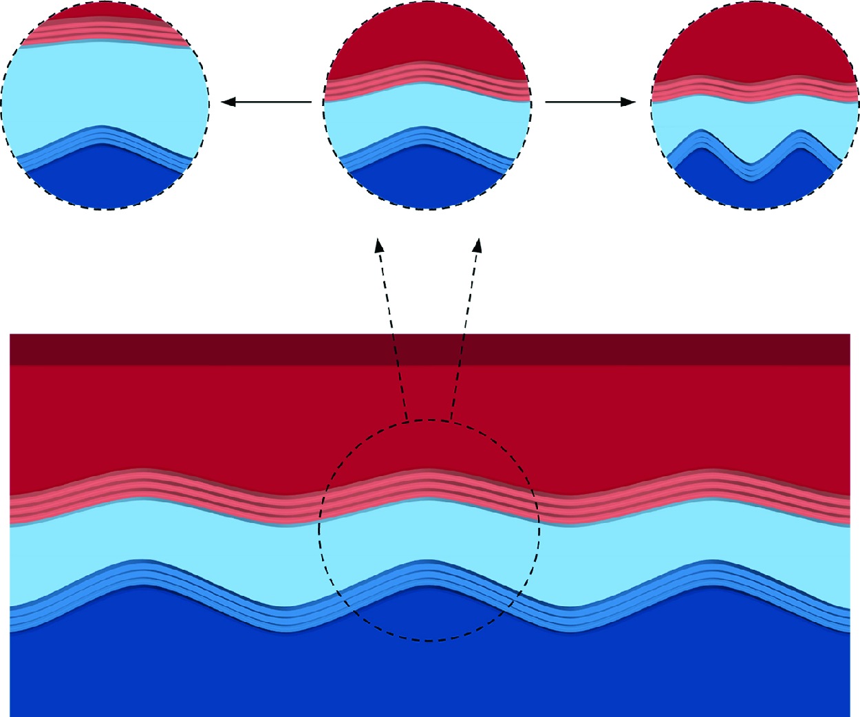
(not shown here for brevity). The formation of the disturbance at Peak 2 is recognised as the propagation of waves at Peak 1 from the ice–water interface to the water–air interface. An increase in the thickness of the water layer results in a reduction of the effect of the perturbation at the ice–water interface to that at the water–air interface through a ‘buffer layer’, i.e. the water. This attenuation of perturbation transmission leads to a weakening of Peak 2, as observed in figure 9. It is worth emphasising that Peak 2 emerges only when Peak 1 is present. In cases where there is no Peak 1 at the ice–water interface, signifying the absence of ice or water, i.e. ice–air or water–air flows, Peak 2 vanishes as well, indicating that unstable perturbations will no longer exist. This conclusion aligns with the findings in figure 7(a–f) (see the horizontal white dotted lines).
(a) The amplitude ratio of Peak 2 to Peak 1, where the points are numerical results, and the lines are the fitting curves. (b) Schematic diagram of the instability over the three phases at different
 $l_{water}$
and
 $\alpha$
.

Finally, it is of interest to establish a theoretical framework for the relations between the two peaks. The amplitude ratio of Peak 2 to Peak 1 (
 $A_2/A_1$
) at different
 $l_{water}$
and
 $\alpha$
is depicted in figure 10(a). Similar to the increase of
 $l_{water}$
, an increase in wavenumber can also lead to the weakening of Peak 2, indicating that perturbations with shorter wavelengths are less able to reach the water–air interface. This is because the viscous diffusion effect within the buffer layer increases with the wavenumber. Such decay with respect to the propagation distance was reported to be exponential in sound wave attenuation (Straka et al. Reference Straka, Meerschaert, McGough and Zhou2013). As
 $l_{water}$
has a similar effect to
 $\alpha$
on the decay, we can expect the function to be fitted as
 $A_2/A_1=B_1 \textrm { exp} (-B_2\alpha l_{water})$
, where
 $B_1=1.34$
and
 $B_2=12.5$
are constants obtained by fitting the numerical results. The comparison between the fitted curves and the numerical results is shown in figure 10(a). The exponential relation also demonstrates that Peak 2 will vanish when the water layer is thick enough, as the perturbations at Peak 1 will be completely absorbed by the thick water. A more intuitive schematic diagram of the perturbation distribution through a thin water layer and the two peaks is shown in figure 10(b), where the thin water layer is deformed by the disturbance at the ice–water interface. This deformation is then transmitted to the water–air interface, demonstrating that the patterns on the ice surfaces shown in figure 1 are concentrated mainly at the ice–water interface as well as the water–air interface for cases with thinner water layer, while the patterns grow only at the ice–water interface when the water layer is thick enough.
7. Conclusions
In summary, we establish a theoretical framework based on the phase-field method to study the morphological patterns on ice surfaces covered by air-surrounded water flows, which takes essential steps towards unravelling the mysteries of natural pattern formation on ice surfaces. The established model is validated by predicting the wavelength of icicle ripples and comparing it against experimental data. Afterwards, the model is utilised to study the ripples on horizontal ice surfaces, e.g. glaciers and icy lakes.
We demonstrate that the emergence of ice ripples is triggered by an instability originating from the phase interfaces. The relationship between the wavenumber and growth rate of infinitesimal perturbations at various ice and water layer thicknesses is then obtained, illustrating that larger
 $l_{ice}$
and
 $l_{water}$
correspond to patterns with larger wavelengths. When
 $l_{ice}$
or
 $l_{water}$
tends to 0, corresponding to the reduction of the three-phase flow to ice–air or water–air flow, the instability vanishes. The computational results predict dominant wavelength 90 mm, aligning with the observations of the patterns on the ice surface. This wavelength can be used to model the surface roughness and also shed light on the resolution requirement in numerical simulations of icing over complex geometries.
Considering that gravity is critical to trigger the instability, and ice is lighter than liquid water, the present instability is analogous to the R–T instability. In contrast to gravity, our results show that surface tension and viscosity serve to suppress the instability. The predicted dominant wavelength 90 mm is also consistent with the typical R–T instability theory. It is worth noting that our model can be applied not only in analysing the gravity-driven R–T type instability, but also in studying other kinds of instabilities, such as icicle ripples driven by surface flows. Furthermore, the ability to handle three-phase flows with phase changes, and to analyse the effects of water and ice thicknesses on the dominant wavelength, highlights the advantages of our model over the typical R–T theory.
Moreover, based on our three-phase model, the profiles of the perturbations are presented, primarily illustrating two peaks concentrated at the ice–water and water–air interfaces. Furthermore, a theoretical framework is established to explain the exponential-form correlation between the amplitudes of the two peaks with respect to
 $l_{water}$
and wavenumber
 $\alpha$
.
Overall, this linear stability research contributes to the fundamental understanding of the mechanism of pattern formation on the ice surface, and paves the way for further studies on the impact of wind speed, temperature, pressure, other surface conditions and nonlinear interactions on the icing process.
Funding
This work was supported by the China Scholarship Council, the National Natural Science Foundation of China (grant nos 92152109, 11988102), the ARCHER2-eCSE05-6 project, and the EU H2020-MSCA-RISE-2017 project CTFF (Control of Turbulent Friction Force, grant no. 777717).
Declaration of interests
The authors report no conflict of interest.
Data availability statement
The data that support the findings of this study are available from the corresponding author upon request.
Author contributions
Z.W. derived the theory, performed the simulations and formal analysis, wrote the original draft, and created visualisations. K.-S.C. and S.L. contributed to the formal analysis, review and supervision. C.S. contributed to the formal analysis, review and validation. X.M. conceptualised the study, developed the methodology, performed formal analysis and investigation, and contributed to writing, review and supervision.
Appendix A. The stability equation
The non-zero elements in the stability equation (2.10) are given below with
 $\theta$
the inclined angle between the flow direction
 $x$
and the horizontal plane. Here,
 $\theta =0$
is applied for the flows on the horizontal glacier and lake shown in figure 1, while for icicles in § 5,
 $\theta =\pi /2$
is applied since the flows are vertical to the horizontal line. The velocity vector
 $\boldsymbol u'$
is expanded into
 $u^{\prime}_x$
and
 $u^{\prime}_y$
, and
 $u_0$
and
 $v_0$
are used to denote the corresponding base flow velocities, respectively. We note that the base flow is steady (
 ${\partial \boldsymbol{q}_0}/{\partial t}=0$
) and independent of
 $x$
(
 ${\partial \boldsymbol{q}_0}/{\partial x}=0$
), and the base velocity is parallel to the
 $x$
direction (
 $v_0=0$
).
 \begin{gather} \boldsymbol{\Gamma }(1,1)=\boldsymbol{\Gamma }(2,2)=-\rho _0, \nonumber \\[3pt] \boldsymbol{\Gamma }(3,4)=\tfrac {1}{2}(\phi _0+1)(\rho _l-\rho _s), \nonumber \\[3pt] \boldsymbol{\Gamma }(3,5)=\tfrac {1}{2}[(c_0+1)\rho _l-c_0\rho _s-\rho _g)], \nonumber \\[3pt] \boldsymbol{\Gamma }(4,4)=\boldsymbol{\Gamma }(5,5)=1, \nonumber \\[3pt] \boldsymbol{\Gamma }(7,4)=-\frac {1}{2}(\phi _0+1)L -\frac {1}{2}c_{p0}T_0[(\phi _0+1)(\rho _l-\rho _s)] \nonumber \\[3pt] -\frac {1}{2}\rho _0T_0[(\phi _0+1)(c_{pl}-c_{ps})], \nonumber \\[3pt] \boldsymbol{\Gamma }(7,5)=-\frac {1}{2}c_0L -\frac {1}{2}c_{p0}T_0[(c_0+1)\rho _l-c_0\rho _s-\rho _g] \nonumber \\[3pt] -\frac {1}{2}\rho _{0}T_0[(c_0+1)c_{pl}-c_0c_{ps}-c_{pg}], \nonumber \\[3pt] \boldsymbol{\Gamma }(7,7)=-\rho _0c_{p0}, \end{gather}
 \begin{gather}\boldsymbol{H}_x(1,1)= -\rho _0 u_0, \nonumber \\[3pt] \boldsymbol{H}_x(1,2)= \frac {1}{\textit{Re}}\frac {\partial \mu _0}{\partial y}, \nonumber \\[1pt] \boldsymbol{H}_x(1,3)=-1, \nonumber \\[1pt] \boldsymbol{H}_x(1,4)=-\frac {3}{2\sqrt {2}}\frac {Cn_{1}}{We_1}\frac {\partial ^2 c_0}{\partial y^2}, \nonumber \\[3pt] \boldsymbol{H}_x(1,5)=-\frac {3}{2\sqrt {2}}\frac {Cn_{2}}{We_2}\frac {\partial ^2 \phi _0}{\partial y^2}, \nonumber \end{gather}\begin{gather} \boldsymbol{H}_x(2,1)=-\frac {2}{3}\frac {1}{\textit{Re}}\frac {\partial \mu _0}{\partial y}, \nonumber \\[1pt]\boldsymbol{H}_x(2,2)=-\rho _0 u_0, \nonumber \\[1pt]\boldsymbol{H}_x(2,4)=\frac {1}{2}\frac {1}{\textit{Re}}\frac {\partial u_0}{\partial y}(\phi _0+1)(\mu _l-\mu _s), \nonumber \\[3pt] \boldsymbol{H}_x(2,5)=\frac {1}{2}\frac {1}{\textit{Re}}\frac {\partial u_0}{\partial y}[(c_0+1)\mu _l-c_0\mu _s-\mu _g], \ \ \ \ \ \ \ \ \ \nonumber \\[3pt] \boldsymbol{H}_x(3,1)=\rho _0, \nonumber \\[3pt] \boldsymbol{H}_x(3,4)=\tfrac {1}{2}u_0(\phi _0+1)(\rho _l-\rho _s), \nonumber\\[3pt]\boldsymbol{H}_x(3,5)=\tfrac {1}{2}u_0[(c_0+1)\rho _l-c_0\rho _s-\rho _g], \nonumber \\[3pt] \boldsymbol{H}_x(4,1)=c_0, \nonumber \\[3pt] \boldsymbol{H}_x(4,4)=\boldsymbol{H}_x(5,5)=u_0, \nonumber \\[3pt] \boldsymbol{H}_x(7,1)=-\rho _0 c_{p0}T_0, \nonumber \\[3pt] \boldsymbol{H}_x(7,2)=2\frac {Ec}{\textit{Re}}\mu _0\frac {\partial u_0}{\partial y}, \nonumber \\[3pt] \boldsymbol{H}_x(7,4)=-\frac {1}{2}c_{p0}T_0u_0(\phi _0+1)(\rho _l-\rho _s) \nonumber \\[3pt] -\frac {1}{2}\rho _0T_0u_0(\phi _0+1)(c_{pl}-c_{ps}), \nonumber \\[3pt] \boldsymbol{H}_x(7,5)=-\frac {1}{2}c_{p0}T_0u_0[(c_0+1)\rho _l-c_0\rho _s-\rho _g] \nonumber \\[3pt] -\frac {1}{2}\rho _0T_0u_0[(c_0+1)c_{pl}-c_0c_{ps}-c_{pg}], \nonumber \\[3pt] \boldsymbol{H}_x(7,7)=-\rho _0c_{p0}u_0, \end{gather}
 \begin{gather} \boldsymbol{H}_y(1,1)=\frac {1}{\textit{Re}}\frac {\partial \mu _0}{\partial y}, \nonumber \\[3pt] \boldsymbol{H}_y(1,4)=\frac {1}{2}\frac {1}{\textit{Re}}\frac {\partial u_0}{\partial y}(\phi _0+1)(\mu _l-\mu _s), \nonumber \\[3pt] \boldsymbol{H}_y(1,5)=\frac {1}{2}\frac {1}{\textit{Re}}\frac {\partial u_0}{\partial y}[(c_0+1)\mu _l-c_0\mu _s-\mu _g], \nonumber \\[3pt] \boldsymbol{H}_y(2,2)=\frac {4}{3}\frac {1}{\textit{Re}}\frac {\partial \mu _0}{\partial y}, \nonumber \\[3pt] \boldsymbol{H}_y(2,3)=-1, \nonumber \\[3pt] \boldsymbol{H}_y(2,4)=-\frac {3}{2\sqrt {2}}\frac {Cn_{1}}{We_1}\frac {\partial ^2 c_0}{\partial y^2}, \nonumber \\[3pt] \boldsymbol{H}_y(2,5)=-\frac {3}{2\sqrt {2}}\frac {Cn_{2}}{We_2}\frac {\partial ^2 \phi _0}{\partial y^2}, \nonumber \end{gather}\begin{gather}\boldsymbol{H}_y(3,2)=\rho _0, \nonumber \\[1pt] \boldsymbol{H}_y(4,2)=c_0, \nonumber \\[3pt] \boldsymbol{H}_y(7,1)=2\frac {Ec}{\textit{Re}}\mu _0\frac {\partial u_0}{\partial y}, \nonumber \\[3pt] \boldsymbol{H}_y(7,2)=-\rho _0 c_{p0}T_0, \nonumber \\[3pt]\boldsymbol{H}_y(7,4)=\frac {1}{2}\frac {1}{\textit{Re}\,Pr}\frac {\partial T_0}{\partial y}(\phi _0+1)(\kappa _l-\kappa _s), \nonumber \\[3pt] \boldsymbol{H}_y(7,5)=\frac {1}{2}\frac {1}{\textit{Re}\,Pr}\frac {\partial T_0}{\partial y}[(c_0+1)\kappa _l-c_0\kappa _s-\kappa _g], \ \ \ \ \ \ \ \nonumber \\[3pt] \boldsymbol{H}_y(7,7)=\frac {1}{\textit{Re}\,Pr}\frac {\partial \kappa _0}{\partial y}, \end{gather}
 \begin{gather} \boldsymbol{H}(1,2)=-\rho _0\frac {\partial u_0}{\partial y}, \nonumber \\[3pt] \boldsymbol{H}(1,4)=\frac {1}{2}\frac {1}{\textit{Re}}\frac {\partial u_0}{\partial y}\frac {\partial \phi _0}{\partial y}(\mu _l-\mu _s) +\frac {1}{2}\frac {1}{\textit{Re}}\frac {\partial ^2 u_0}{\partial y^2}(\phi _0+1)(\mu _l-\mu _s) \nonumber \\[3pt] +\frac {1}{2}\frac {\textrm { sin} \hspace {0.1 em} \theta }{\textit{Fr}^2}(\phi _0+1)(\rho _l-\rho _s), \nonumber \\[3pt] \boldsymbol{H}(1,5)=\frac {1}{2}\frac {1}{\textit{Re}}\frac {\partial u_0}{\partial y}\frac {\partial c_0}{\partial y}(\mu _l-\mu _s) +\frac {1}{2}\frac {1}{\textit{Re}}\frac {\partial ^2 u_0}{\partial y^2}[(c_0+1)\mu _l-c_0\mu _s-\mu _g] \nonumber \\[3pt] +\frac {1}{2}\frac {\textrm { sin}\hspace {0.1 em}\theta }{\textit{Fr}^2}[(c_0+1)\rho _l-c_0\rho _s-\rho _g], \nonumber \\[3pt] \boldsymbol{H}(2,4)=-\frac {1}{2}\frac {\textrm { cos}\hspace {0.1 em} \theta }{\textit{Fr}^2}(\phi _0+1)(\rho _l-\rho _s), \nonumber \\[3pt] \boldsymbol{H}(2,5)=-\frac {1}{2}\frac {\textrm { cos}\hspace {0.1 em} \theta }{\textit{Fr}^2}[(c_0+1)\rho _l-c_0\rho _s-\rho _g], \nonumber \\[3pt] \boldsymbol{H}(3,2)=\frac {\partial \rho _0}{\partial y}, \nonumber \\[3pt] \boldsymbol{H}(4,2)=\frac {\partial c_0}{\partial y}, \nonumber \\[3pt] \boldsymbol{H}(4,4)=\frac {M_{nc}}{Cn_1}(6c^2_0 +6c_0+1) -2M_{nl}(T_0-1)c_0(c_0+1)(2c_0+1), \nonumber \\[3pt] \boldsymbol{H}(4,7)=-M_{nl}c^2_0(c_0+1)^2, \nonumber \\[3pt] \boldsymbol{H}(5,2)=\frac {\partial \phi _0}{\partial y}, \nonumber \\[3pt] \boldsymbol{H}(6,5)=\frac {1-3\phi _0^2}{Cn_{2}}, \nonumber \\[3pt] \boldsymbol{H}(6,6)=1, \nonumber \\[3pt] \boldsymbol{H}(7,1)=\frac {Ec}{\textit{Fr}^2}\rho _0 \textrm { sin}\hspace {0.1 em}\theta , \nonumber \\[3pt] \boldsymbol{H}(7,2)=-\frac {\partial (\rho _0 c_{p0}T_0)}{\partial y} - \frac {Ec}{\textit{Fr}^2}\rho _0 \textrm { cos}\hspace {0.1 em}\theta , \nonumber \\[3pt] \boldsymbol{H}(7,4)=\frac {1}{2}\frac {1}{\textit{Re}\,Pr}\frac {\partial T_0}{\partial y}\frac {\partial \phi _0}{\partial y}(\kappa _l-\kappa _s) + \frac {1}{2}\frac {1}{\textit{Re}\,Pr}\frac {\partial ^2 T_0}{\partial y^2}(\phi _0+1)(\kappa _l-\kappa _s) \nonumber \\[3pt] + \frac {1}{2}\frac {Ec}{\textit{Re}}(\frac {\partial u_0}{\partial y})^2(\phi _0+1)(\mu _l-\mu _s) \nonumber \\[3pt] + \frac {1}{2}\frac {Ec}{\textit{Fr}^2}u_0\textrm { sin}\hspace {0.1 em}\theta (\phi _0+1)(\rho _l-\rho _s), \nonumber \end{gather}\begin{gather}\boldsymbol{H}(7,5)=\frac {1}{2}\frac {1}{\textit{Re}\,Pr}\frac {\partial T_0}{\partial y}\frac {\partial c_0}{\partial y}(\kappa _l-\kappa _s) + \frac {1}{2}\frac {1}{\textit{Re}\,Pr}\frac {\partial ^2 T_0}{\partial y^2}[(c_0+1)\kappa _l-c_0\kappa _s-\kappa _g] \nonumber \\[3pt] + \frac {1}{2}\frac {Ec}{\textit{Re}}(\frac {\partial u_0}{\partial y})^2[(c_0+1)\mu _l-c_0\mu _s-\mu _g] \nonumber \\[3pt] + \frac {1}{2}\frac {Ec}{\textit{Fr}^2}u_0\textrm { sin}\hspace {0.1 em}\theta [(c_0+1)\rho _l-c_0\rho _s-\rho _g], \end{gather}
 \begin{gather} \boldsymbol{H}_{xx}(1,1)=\frac {4}{3}\frac {\mu _0}{\textit{Re}}, \nonumber \\[3pt] \boldsymbol{H}_{xx}(2,2)=\frac {\mu _0}{\textit{Re}}, \nonumber \\[3pt] \boldsymbol{H}_{xx}(2,4)=-\frac {3}{2\sqrt {2}}\frac {Cn_{1}}{We_1}\frac {\partial c_0}{\partial y}, \nonumber \\[3pt] \boldsymbol{H}_{xx}(2,5)=-\frac {3}{2\sqrt {2}}\frac {Cn_{2}}{We_2}\frac {\partial \phi _0}{\partial y}, \nonumber \\[3pt] \boldsymbol{H}_{xx}(4,4)=-M_{nc}Cn_1, \nonumber \\[3pt] \boldsymbol{H}_{xx}(5,6)=-M_{n\phi }, \nonumber \\[3pt] \boldsymbol{H}_{xx}(6,5)=Cn_2, \nonumber \\[3pt] \boldsymbol{H}_{xx}(7,7)=\frac {\kappa _0}{\textit{Re}\,Pr}, \end{gather}
 \begin{gather} \boldsymbol{H}_{yy}(1,1) = \frac {\mu _0}{\textit{Re}}, \nonumber \\[3pt] \boldsymbol{H}_{yy}(2,2) = \frac {4}{3}\frac {\mu _0}{\textit{Re}}, \nonumber \\[3pt] \boldsymbol{H}_{yy}(2,4) = -\frac {3}{2\sqrt {2}}\frac {Cn_{1}}{We_1}\frac {\partial c_0}{\partial y}, \nonumber \\[3pt] \boldsymbol{H}_{yy}(2,5) = -\frac {3}{2\sqrt {2}}\frac {Cn_{2}}{We_2}\frac {\partial \phi _0}{\partial y}, \nonumber \\[3pt] \boldsymbol{H}_{yy}(4,4) = -M_{nc}Cn_1, \nonumber \\[3pt] \boldsymbol{H}_{yy}(5,6) = -M_{n\phi }, \nonumber \\[3pt] \boldsymbol{H}_{yy}(6,5) = Cn_2, \nonumber \\[3pt] \boldsymbol{H}_{yy}(7,7) = \frac {\kappa _0}{\textit{Re}\,Pr}, \end{gather}
 \begin{gather} \boldsymbol{H}_{xy}(1,2)=\boldsymbol{H}_{xy}(2,1)=\frac {1}{3}\frac {\mu _0}{\textit{Re}}. \end{gather}
Here,
 $\textit{Re}$
denotes the Reynolds number,
 $\textit{Fr}$
is the Froude number,
 $Pr$
is the Prandtl number,
 $Ec$
is the Eckert number,
 $We_1$
and
 $We_2$
are Weber numbers,
 $Cn_1$
and
 $Cn_2$
represent the Cahn numbers, and
 $ M_{nc}$
,
 $M_{n\phi }$
and
 $M_{nl}$
denote the mobility numbers. These numbers are defined as
 \begin{align} &\textit{Re}=\frac {\rho _{r}u_{r}d_r}{\mu _{r}},\quad \textit{Fr}=\frac {u_{r}}{\sqrt {gd_r}},\quad Pr=\frac {\mu _{r}c_{pr}}{\kappa _{r}},\quad Ec=\frac {u^{2}_{r}}{c_{pr}T_{r}}, \nonumber \\ & We_1=\frac {u^{2}_{r}\rho _{r}d_r}{\sigma _{c}},\quad We_2=\frac {u^{2}_{r}\rho _{r}d_r}{\sigma _{\phi }},\quad Cn_1=\frac {\xi _c}{d_r},\quad Cn_2=\frac {\xi _\phi }{d_r}, \nonumber \\ & M_{nc}=\frac {6M_c\sigma _c}{u_{r}},\quad M_{n\phi }=\frac {3M_\phi \sigma _\phi }{2\sqrt {2} u_{r}d^{2}_r},\quad M_{nl}=\frac {30M_cLd_r}{u_{r}}, \end{align}
where the subscript
 $r$
denotes the reference values,
 $d_r$
,
 $u_{r}$
and
 $T_r=T_M$
represent the reference thickness, the reference velocity and the reference temperature, respectively, and
 $\boldsymbol{u}, t, p, \rho , T, \mu , \kappa , c_p$
,
 $\boldsymbol{\nabla}$
and
 $L$
are non-dimensionalised by
 $u_r$
,
 $d_r/u_r$
,
 $\rho _r u^2_r$
,
 $\rho _r$
,
 $T_r$
,
 $\mu _r$
,
 $\kappa _r$
,
 $c_{pr}$
,
 $d_r$
and
 $\rho _r c_{pr}T_r$
, respectively.



