


1. Introduction
For wall-bounded turbulence, the attached-eddy hypothesis (AEH) might be one of the most successful theoretical frameworks that attempts to bridge the gap between the statistical and the structural perspectives on inertial turbulent motions, which make the leading-order contribution to the kinematics and dynamics of wall-bounded turbulence.
In the original hypothesis (Townsend & Batchelor Reference Townsend and Batchelor1951; Townsend Reference Townsend1961, Reference Townsend1976), inertial coherent motions in wall-bounded turbulence at asymptotically high Reynolds number can be modelled by a hierarchy of randomly distributed attached eddies (AEs). These energy-containing eddies are self-similar in geometries and are attached to the wall. The term ‘attach’, according to Marusic & Monty (Reference Marusic and Monty2019), describes that the velocity fields induced by AEs are influenced by the wall but might not be physically connected to it. The concept of AEs was successfully embodied by Perry and his co-authors (Perry & Chong Reference Perry and Chong1982; Perry, Henbest & Chong Reference Perry, Henbest and Chong1986; Perry & Marusic Reference Perry and Marusic1995) as discrete  $\varLambda$-shaped line vortices with various scales, which perturb the mean flow through the vortex induction effect prescribed by the Biot–Savart law. The linear superposition of a hierarchy of them well restores the logarithmic law of both the mean velocity profile
 $\bar {U}(y)$ and the profile of the variance of the streamwise fluctuating velocity
 $\langle u^{2} \rangle (y)$. A
 $-1$ scaling of the streamwise spectrum, i.e.
 $\varPhi _{uu} \propto k_x^{-1}$, in the inertial-scale subrange was further predicted at asymptotically high Reynolds number (
 $Re$).
AEH has received growing support from both experiments and simulations. Nowadays, it is well accepted that AEs are closely related to the observed scaling behaviours of various statistical quantities, including even-order moments of the streamwise fluctuating velocity, velocity correlation function and moment generating function (Marusic et al. Reference Marusic, Monty, Hultmark and Smits2013; Meneveau & Marusic Reference Meneveau and Marusic2013; Stevens, Wilczek & Meneveau Reference Stevens, Wilczek and Meneveau2014; de Silva et al. Reference de Silva, Marusic, Woodcock and Meneveau2015; Yang et al. Reference Yang, Baidya, Johnson, Marusic and Meneveau2017). Recently, Hwang & Lee (Reference Hwang and Lee2020b) analytically demonstrated that the existence of self-similar AEs is a necessary and sufficient condition for the existence of the log law of the mean velocity profile. Although AEH is proposed based on an asymptotic assumption, a bulk of studies (Deng et al. Reference Deng, Pan, Wang and He2018; Cheng et al. Reference Cheng, Li, Lozano-Durán and Liu2019; Hwang & Lee Reference Hwang and Lee2020a) have reported the signatures of AEs in the low-to-moderate  $Re$ regime, which, according to Smits, McKeon & Marusic (Reference Smits, McKeon and Marusic2011), is
 $Re_\tau <5000$ (
 $Re_\tau =\delta u_\tau /\nu$, with
 $\delta$ the thickness of a turbulent boundary layer or the half-channel height of a turbulent channel,
 $\nu$ the kinematic viscosity and
 $u_\tau$ the frictional velocity). Nevertheless, due to the insufficient scale separation, the contamination from other kinds of motions such as viscous-scaled random fluctuations or detached eddies were found to bias the log-layer turbulent statistics from those predicted by AEH (Jiménez & Hoyas Reference Jiménez and Hoyas2008; Deshpande, Monty & Marusic Reference Deshpande, Monty and Marusic2019; Deshpande et al. Reference Deshpande, Chandran, Monty and Marusic2020).
The physical representation of AEs is an intriguing question, since it is the key to both understanding the origin of AEs and modelling their spatio-temporal dynamics. Hairpin vortices have been regarded as the physical representations of the conceptual  $\varLambda$ vortices (Balakumar & Adrian Reference Balakumar and Adrian2007; de Silva, Hutchins & Marusic Reference de Silva, Hutchins and Marusic2016a). Considering the remarkable scale separation, individual vortical structures, whose length scales are
 $O(l^{*})$ (
 $l^{*}=\nu /u_\tau$), are unlikely to be the representations of AEs, whose length scales are
 $O(\delta )$. The self-organization of individual vortices into packet-like structures due to either parent–offspring regeneration or preferential alignment (Zhou et al. Reference Zhou, Adrian, Balachandar and Kendall1999; Balakumar & Adrian Reference Balakumar and Adrian2007; Dennis & Nickels Reference Dennis and Nickels2011) provides a mechanism for scale growth. Nevertheless, statistical evidence for the existence of either hairpin vortices or vortex packets is only evident in the low-to-moderate
 $Re$ range at the moment (Ganapathisubramani & Longmire Reference Ganapathisubramani and Longmire2003; Deng et al. Reference Deng, Pan, Wang and He2018; Wang et al. Reference Wang, Gao, Wang, Wang and Pan2019a). Another viewpoint is to treat AEs as a hierarchy of self-sustaining structures spanning from inner-layer velocity streaks and streamwise vortices to outer-layer superstructures (or very-large-scale motions) and large-scale streamwise rollers (Hwang Reference Hwang2013, Reference Hwang2015), the latter of which were thought to originate from the intrinsic outer-layer streak instability that is independent of the inner-layer cycle (Hamilton, Kim & Waleffe Reference Hamilton, Kim and Waleffe1995). It is noted that such a viewpoint is based on a novel numerical experiment that artificially isolated turbulent motions with concerned scales by means of over-damped large eddy simulation (Hwang Reference Hwang2013, Reference Hwang2015). The interaction of resolved turbulent motions with those unresolved ones was implicitly omitted. To what extent the omitted inter-scale interaction will affect the observed AE-like kinematic properties is still an open question.
The fast development of measurement techniques and computational capacities stimulates a growing trend of finding the physical representations of AEs via data-driven techniques. In general, there are two routes along this trend. One is a statistical approach. Namely, particular scale filtering methods are used to decompose full-order velocity fields into scale-separated motions, whose kinematical statistics are then compared with those predicted by AEH. The applied techniques include spectrum-based scale decomposition (Baars, Hutchins & Marusic Reference Baars, Hutchins and Marusic2017; Baars & Marusic Reference Baars and Marusic2020a,Reference Baars and Marusicb; Hu, Yang & Zheng Reference Hu, Yang and Zheng2020; de Silva et al. Reference de Silva, Chandran, Hutchins and Marusic2020), proper orthogonal decomposition (POD) (Hellström, Ganapathisubramani & Smits Reference Hellström, Ganapathisubramani and Smits2015; Hellström, Marusic & Smits Reference Hellström, Marusic and Smits2016), bi-dimensional empirical mode decomposition (Agostini & Leschziner Reference Agostini and Leschziner2016; Cheng et al. Reference Cheng, Li, Lozano-Durán and Liu2019) and variational mode decomposition (Wang, Pan & Wang Reference Wang, Pan and Wang2018, Reference Wang, Pan and Wang2019b). The acquired knowledge is that large-scale motions (LSMs) with streamwise length scale of  $\lambda _x/\delta =0.1{\sim} 3$ roughly restore AEH-predicted statistical behaviours.
Another route is to focus on the structural perspective of AEs. Del Alamo & Zandonade (Reference Del Alamo and Zandonade2006), Lozano-Durán, Flores & Jiménez (Reference Lozano-Durán, Flores and Jiménez2012) and Lozano-Durán & Jimenez (Reference Lozano-Durán and Jimenez2014) used the so-called clustering algorithm to detect instantaneous flow structures from snapshots of velocity fields of turbulent channel flow (TCF) obtained by direct numerical simulation (DNS). Tall attached vortex clusters and quadrant structures associated with sweep and ejection events were found to be self-similar in geometries. Recently, Hwang & Sung (Reference Hwang and Sung2018) applied the clustering algorithm to the DNS dataset of a turbulent boundary layer (TBL) at low  $Re$. Instantaneous streamwise-component velocity structures that are ‘physically’ attached to the wall were deemed as the prime surrogates of AEs. Using this method, similar AE-like velocity structures were subsequently identified in TCF (Cheng et al. Reference Cheng, Li, Lozano-Durán and Liu2020), turbulent pipe flow (Hwang & Sung Reference Hwang and Sung2019), adverse-pressure-gradient TBL flow (Yoon, Hwang & Yang Reference Yoon, Hwang and Yang2020) and travelling wavy boundary flow (Wang et al. Reference Wang, Xu, Sung and Huang2021b). It is noted that, in the present paper, ‘attached’ eddies are used to denote coherent motions conforming to Townsend's AEH; while ‘wall-attached’ ones refer to those structures that are physically connected or close enough to the wall. The same for ‘detached’ and ‘wall-detached’ eddies. According to Baars et al. (Reference Baars, Hutchins and Marusic2017), Hwang & Lee (Reference Hwang and Lee2020a) and Deshpande et al. (Reference Deshpande, Chandran, Monty and Marusic2020), not all ‘wall-attached’ eddies conform to the definition of ‘attached’ eddy.
Despite the substantial evidence for the existence of AEs, there are several issues that should be further addressed before a distinct picture of the physical representation of AEs can be drawn. The statistical route focuses on the statistical behaviour of AE-like turbulent motions. However, their spatio-temporal coherence, which is a key for developing structure-based turbulent models, is usually inaccessible. This constraint becomes more prominent when one-point time series of streamwise velocity measured by hot-wire anemometry are analysed by the scale filtering method. Another limitation is that it is challenging to completely isolate wall-detached motions, which were considered as Type-B eddies by Marusic & Monty (Reference Marusic and Monty2019), from those wall-attached ones via scale filtering in the low-to-moderate  $Re$ regime (Deshpande et al. Reference Deshpande, Chandran, Monty and Marusic2020; Hwang & Lee Reference Hwang and Lee2020a). As for the structural route, the success of using instantaneous wall-attached velocity structures to represent AEs is inspiring. But it is noteworthy that in the original formulation of AEH, ‘the candidate AE to be used in the model is an average of many realizations of instantaneous structures’ (Marusic & Monty Reference Marusic and Monty2019). This reminds us that it is more accurate to interpret AEs as the statistical representations of an ensemble of individual structures with similar kinematic properties.
There is a growing trend of incorporating the statistical and structural perspectives as a whole. Baars and his colleagues developed a spectrum-based filter for velocity decomposition (Baars et al. Reference Baars, Hutchins and Marusic2017; Baars & Marusic Reference Baars and Marusic2020a,Reference Baars and Marusicb). By applying this novel method to multi-point datasets, understandings of the spatial coherence of the Fourier modes of wall-attached motions are significantly promoted (Chandran et al. Reference Chandran, Baidya, Monty and Marusic2017; Baidya et al. Reference Baidya2019; Deshpande et al. Reference Deshpande, Monty and Marusic2019, Reference Deshpande, Chandran, Monty and Marusic2020; Chandran, Monty & Marusic Reference Chandran, Monty and Marusic2020; Deshpande, Monty & Marusic Reference Deshpande, Monty and Marusic2021a). Furthermore, Baidya et al. (Reference Baidya, Philip, Hutchins, Monty and Marusic2017), Eich et al. (Reference Eich, de Silva, Marusic and Kähler2020) and Deshpande et al. (Reference Deshpande, de Silva, Lee, Monty and Marusic2021b) used  $\varLambda$-shaped eddy packets to synthetically reconstruct statistical quantities of inertial motions in wall-bounded turbulence.
Following these works, the present study aims to extract the physical representations of AEs from velocity fields of TBLs at low-to-moderate  $Re$ via a data-driven method. Both the statistical signature of AEs in the scale spectrum and their spatial coherence in physical space are to be sought. The technique of POD is used as the mode decomposition method to extract coherent motions from planar velocity fields in the streamwise–wall-normal plane of TBLs, which were obtained by either two-dimensional (2-D) planar particle image velocimetry (PIV) measurement with large field of view (FOV) or DNS. The reason for choosing POD as the mode decomposition method is that POD decomposes full-order velocity fields into discrete orthogonal modes not by scales but by energy contents. This is consistent with the assumption that AEs have constant energy density so that their contributions to the total turbulent kinetic energy (TKE) are proportional to their size. Furthermore, POD mode functions reveal the spatial coherence of particular turbulent motions in an average sense, thus are possible to represent the statistical patterns of AEs.
The remaining part of this paper is organized as follows. The details of the TBL datasets to be analysed will be described in § 2. The geometric characteristics of leading-order POD modes, as well as their scale and energy hierarchy, will be presented in § 3. In addition, the statistical property of POD modes and the classification of POD eddies will be described. In § 4, the kinematical properties of wall-attached POD eddies, including their contribution to the logarithmic scaling of the variance of the streamwise fluctuating velocity and the related one-dimensional (1-D) streamwise spectrum, will be examined in detail. As a comparison, those kinematical properties contributed by either superstructures or wall-detached POD eddies will be also presented. The quasi-Gaussian behaviour of wall-attached POD eddies will be further discussed in § 5 by analysing the scaling of high-even-order moments, moment generating functions (MGF) and high-order two-point structural functions (SFs). Concluding remarks are to be drawn in § 6. Furthermore, Appendices A and B will discuss the effect of the streamwise size of the FOV and the wall-attachment condition in the eddy detection algorithm on the statistics of wall-attached POD eddies, respectively.
The nomenclature is as follows. The superscript  $^{+}$ represents a quantity being normalized by either the wall unit
 $l^{*}$ or frictional velocity
 $u_\tau$. The angled bracket
 $\langle {\cdot }\rangle$ indicates ensemble average;
 $x/y/z$ denotes the streamwise/wall-normal/spanwise direction, respectively.
 $U/V/W$ is the corresponding instantaneous velocity and
 $u/v/w$ is the fluctuating component.
2. Datasets of TBL
In the present study, three TBL datasets in the range of  $Re_\tau =\delta u_\tau /\nu \approx 1200{\sim} 4300$ are used for data-driven analysis. Two were obtained by 2-D planar PIV measurement of the streamwise–wall-normal plane of a spatially developing TBL in either a water channel (WC) or a wind tunnel (WT), another one is an open-source DNS dataset (Borrell, Sillero & Jiménez Reference Borrell, Sillero and Jiménez2013; Sillero, Jiménez & Moser Reference Sillero, Jiménez and Moser2013). Hereinafter, they are denoted as Cases WC, WT and DNS, respectively.
The WC dataset was obtained in a low-speed recirculating water channel in Beihang University, whose test section has a size of  $3.0\times 0.6\times 0.7$ m (length
 $\times$ width
 $\times$ height). A smooth glass plate with a length of 3 m, a width of 0.6 m and a thickness of 5 mm was laid on the bottom wall of this water channel for the development of a smooth-wall TBL. The leading edge of this plate was bevelled to a ramp with a length of 45 mm to prevent local flow separation. A tripping wire with a diameter of 3 mm was fixed on the working surface at 200 mm downstream of the leading edge to trip the boundary layer transition. In the PIV measurement, hollow glass beads with a median diameter of 10
 $\mathrm {\mu }$m and a mean density of 1.05 g cm
 $^{-3}$ were seeded in the flow as tracer particles. The symmetric streamwise–wall-normal plane of the test section was illuminated by a laser sheet with a thickness of approximately 1 mm, which was emitted from a dual-pulsed Nd:YAG laser generator (Beamtech Vlite-380, Beamtech, China) at an energy output of 300 mJ/pulse. Four wide-format straddle-frame CCD cameras (Imperx CLB-B6620M, Imperx, USA), each of which had a resolution of
 $6600\times 4400$ pixels, were aligned along the streamwise direction to image the 2-D flow field synchronously. The streamwise FOVs of neighbouring cameras have an overlap of 15 mm to facilitate the stitching of multi-view velocity fields. Such a multi-camera PIV configuration was designed to cover a total FOV of
 ${\rm \Delta} X\times {\rm \Delta} Y=655\times 175\ {\rm mm}^{2}$ (or
 $10.6\delta \times 1.8\delta$) while keeping the spatial resolution of the velocity fields to
 ${\rm \Delta} x^{+} \mid {\rm \Delta} y^{+}=O(10)$. The middle of the FOV was located at
 $x=1900$ mm downstream of the tripping wire. Owing to the large streamwise span of the FOV, the frictional Reynolds number varied from
 $Re_\tau =1100$ at the inlet of the FOV to
 $Re_\tau =1300$ at the outlet when the free-stream velocity was
 $U_\infty =485$ mm s
 $^{-1}$. The spatial developing nature as well as its effect on the kinematic statistics, will be addressed later. It is noted that a similar multi-camera PIV configuration has been successfully used in de Silva et al. (Reference de Silva, Chandran, Hutchins and Marusic2020) and Zhu et al. (Reference Zhu, Pan, Wang, Liang, Ji and Wang2021). The advantage is that instantaneous turbulent structures within a large scale range can be well resolved. The limitation is that the measured velocity fields are two-dimensional.
The WT dataset was obtained in a low-speed suction-type wind tunnel in Beihang University. The test section of this wind tunnel has a size of 430 mm (width)  $\times$ 500 mm (height). Its floor is made of glass panels, on the top of which a TBL was tripped by a tripping wire with a diameter of 3 mm at the inlet of the test section. Similar to the measurement of the WC dataset, a multi-camera PIV system with three streamwise-aligned CCD cameras was adopted. The FOV of the PIV measurement was
 ${\rm \Delta} X\times {\rm \Delta} Y=580\times 130\ {\rm mm}^{2}$ (or
 $4.6\delta \times 1.03\delta$), the middle of which was located at 2250 mm downstream of the tripping wire. The free-stream velocity of the air flow was
 $U_\infty =14.95$ m s
 $^{-1}$, and the frictional Reynolds number in the FOV was
 $Re_\tau = 4200{\sim} 4300$.
For Case WC, 2000 statistically independent snapshots of velocity fields were sampled at a repetition rate of 0.75 Hz, covering an eddy turnover time of  $Tu_\tau /\delta =870$. While in Case WT, the PIV system sampled 3600 snapshots at a repetition rate of 1 Hz and a time duration of
 $Tu_\tau /\delta =14\ 660$. Two-dimensional in-plane velocity fields were calculated from particle image pairs by the state-of-the-art optical flow solver based on the Lucas–Kanade algorithm (Pan et al. Reference Pan, Xue, Yang, Wang and Wei2015). Owing to the ultra-high resolution (about
 $29\times 10^{6}$ pixels) of the CCD camera, the size of the final-pass interrogation window was set as
 $48\times 48$ pixels to achieve a high dynamic velocity range. The spatial resolution was approximately
 $16.2\times 16.2$ wall units/vector for Case WC and
 $23.7\times 23.7$ wall units/vector for Case WT. The maximum straddle-frame particle offset was kept as
 $15{\sim} 17$ pixels in the image plane, and the relative error of the velocity measurement was estimated to be less than
 $1\,\%$.
To provide a reference baseline for Case WC, the DNS database of a spatial developing zero-pressure-gradient TBL was also analysed. This database was simulated by Borrell et al. (Reference Borrell, Sillero and Jiménez2013) and Sillero et al. (Reference Sillero, Jiménez and Moser2013). It has been widely used as a benchmark in various studies (Deshpande et al. Reference Deshpande, Monty and Marusic2019; Baars & Marusic Reference Baars and Marusic2020a,Reference Baars and Marusicb; Wang et al. Reference Wang, Gao, Wang, Pan and Wang2020, Reference Wang, Gao, Wang, Pan and Wang2021a). A total of 1700 snapshots of planar velocity fields in the streamwise–wall-normal plane are sliced from 28 volumetric DNS datasets at a spanwise interval of  ${\rm \Delta} z^{+}\approx 250$. The time gap between neighbouring DNS volume blocks is approximately
 ${\rm \Delta} t^{+}=87$ and the time duration of the whole ensemble is
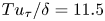 $Tu_\tau /\delta =11.5$. The statistical convergence condition of this DNS dataset has been validated by Sillero et al. (Reference Sillero, Jiménez and Moser2013). The FOV of the sliced plane is
 ${\rm \Delta} X\times {\rm \Delta} Y=10.6\delta \times 1.36\delta$ and the frictional Reynolds number is
 $Re_\tau = 1300{\sim} 1500$, both of which are close to those in Case WC.
Table 1 summarizes the characteristic boundary layer parameters of all three cases, in which the frictional Reynolds number  $Re_\tau$, the momentum Reynolds number
 $Re_\theta$ and the shape factor
 $H$ were estimated by fitting the mean streamwise velocity profiles
 $\bar {U}(y)$ to the canonical composite velocity profile (Chauhan et al. Reference Chauhan, Monkewitz and Nagib2009). As shown in table 1,
 $Re_\tau$ in three cases increases by approximately
 $4.8\,\%{\sim} 18.2\,\%$ across the whole streamwise span (
 ${\rm \Delta} X$) of the FOV, while
 $H$ decreases by
 $0.3\,\%{\sim} 0.8\,\%$. This indicates that the spatially developing nature of the TBL is non-negligible over the FOV. Therefore, if without explicit claim, the local statistics of the flow-field quantities to be presented in the following were calculated at the middle
 $x$ station of the FOV with a short bin of
 $2\delta$, within which the local quasi-parallel condition can be roughly satisfied.
Characteristic parameters of all three TBLs studied here. The characteristic boundary layer thickness  $\delta$ takes the value at the middle
 $x$ station of the FOV.

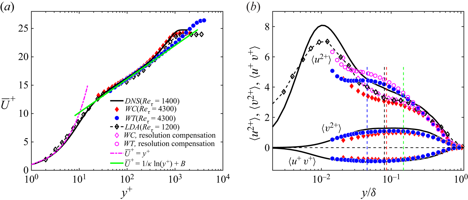
Figure 1 shows the wall-normal profiles of both the mean streamwise velocities and the Reynolds stress, i.e.  $\overline {U}^{+}$,
 $\langle u^{2+} \rangle$,
 $\langle v^{2+} \rangle$ and
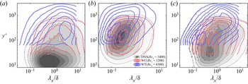
 $\langle u^{+}v^{+} \rangle$, of all three cases. Figure 2 shows the pre-multiplied 1-D spectrograms
 $k_x\varPhi _{uu}(\lambda _x, y)$ and
 $k_x\varPhi _{vv}(\lambda _x, y)$ of
 $u$ and
 $v$, as well as the co-spectra
 $k_x\varPhi _{uv}(\lambda _x, y)$. Noting that these spectra are directly calculated from
 $u(x)$ and
 $v(x)$ over the whole
 $x$ span of the FOV without invoking Taylor's frozen hypothesis. The non-parallel condition of the mean flow is ignored as a leading-order approximation.
Wall-normal variation of single-point turbulent statistics in TBLs of all three datasets at the middle  $x$ station of the FOV. (a) Inner-scaled mean streamwise velocity vs inner-scaled
 $y$. The constants of the logarithmic law that is indicated by the green bold line are
 $\kappa =0.384$ and
 $B=4.17$ (Chauhan, Monkewitz & Nagib Reference Chauhan, Monkewitz and Nagib2009). (b) Inner-scaled Reynolds stress vs outer-scaled
 $y$. In (b), vertical dashed lines in black, red and blue indicate the lower bound of mean-flow log layer in Cases DNS, WC and WT, respectively, while the vertical dash-dotted line in green indicates the upper bound, the same as in figures 8–10, 13, 19 and 21. The
 $y$ range of the mean-flow log layer is
 $3\sqrt {Re_{\tau }}< y^{+}<0.15 \delta ^{+}$ (Marusic et al. Reference Marusic, Monty, Hultmark and Smits2013).

Pre-multiplied streamwise 1-D spectra or co-spectra; (a)  $k_x\varPhi _{uu}(\lambda _x, y)$, (b)
 $k_x\varPhi _{vv}(\lambda _x, y)$ and (c)
 $k_x\varPhi _{uv}(\lambda _x, y)$. Case DNS, Case WC and Case WT are denoted by grey scale patches, dashed contours in red and solid contours in blue, respectively. The spectra are normalized by their maximum value beyond
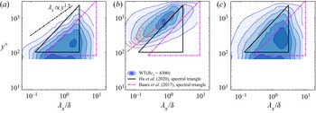
 $y^{+}=40$, and the iso-contours are plotted at the level of 0.15 : 0.15 : 1.2. The magenta dash-doted and black solid triangles in (a) indicate the spectral triangle of (4.4) (proposed by Baars et al. Reference Baars, Hutchins and Marusic2017) and (4.5) (proposed by Hu et al. Reference Hu, Yang and Zheng2020) in Case WT, respectively. It is noted that the streamwise spectra were calculated from
 $u(x)$ or
 $v(x)$ over the whole
 $x$ span of the FOV, the same as in figure 11, 12, 20 and 22.

For Case WC, the PIV-measured streamwise turbulence intensity  $\langle u^{2+} \rangle$ (shown in figure 1b) in the near-wall region (below
 $y^{+}<150$) was insufficiently resolved if compared with those in the DNS case. In contrast,
 $\langle u^{2+} \rangle$ being measured by 1-D laser Doppler anemometry (LDA, Dantec Flow Explorer, Dantec, Denmark) with a probing diameter of 1.0 mm (also shown in figure 1b) is closer to that of Case DNS. The underestimation of
 $\langle u^{2+} \rangle$ in the PIV measurement is due to both the comparably lower spatial resolution of the optical system and the spanwise averaging effect related to the finite laser-sheet thickness. The streamwise spectra (shown in figure 2a) indicate that the underestimation is mainly confined to the small-scale range of
 $\lambda _x<0.4\delta$ for
 $y^{+}>100$; meanwhile, the energy content in the large-scale regime is sufficiently resolved. Case WT faces the same problem. Additionally, the lower part of the buffer layer cannot be reliably measured due to the wall contamination of the illuminating light. Figure 1(b) supplements the resolution-compensated profiles processed by the correction method of Lee et al. (Reference Lee, Kevin, Monty and Hutchins2016). This correction method assumes that the under-resolved small-scale energy is
 $Re$-independent and is linearly correlated with the spatial resolution. Its validity has been checked in TBL with
 $Re_\tau =900{\sim} 6700$ (Lee et al. Reference Lee, Kevin, Monty and Hutchins2016). Figure 1(b) shows that the compensated profile of
 $\langle u^{2} \rangle (y)$ of Case WC is restored to that obtained by LDA. Noting that, in the following analysis, full-order
 $u$ are not processed by this resolution compensation method.
There are three issues that need to be clarified before analysing the obtained datasets. Firstly, in spite of the resolution limitation, it is not small-scale random fluctuations but large-scale coherent motions we are primarily concerned with here. The latter were faithfully captured by the present large-FOV PIV configuration, as can be evidenced by the satisfying agreement of the large-scale part of  $k_x\varPhi _{uu}$ in Case WC and Case DNS with similar
 $Re_\tau$. As will be shown in § 4.1, for Case WC and Case DNS, the profiles of the variance of the streamwise fluctuating velocity contributed by wall-attached POD eddies collapse onto each other in the mean-flow log layer. This demonstrates that the underestimation of small-scale energy content will not bias the statistical signatures of AEs. Secondly, Case WT has a streamwise FOV (
 ${\rm \Delta} X=4.6\delta$) considerably smaller than that of Case WC (
 ${\rm \Delta} X=10.6\delta$). The empirical test in Appendix A will show that the influence of the streamwise FOV on the kinematic statistics of AE-like turbulent motions is weak. Lastly, as a first attempt, only AE-like turbulent motions embedded in
 $u$ component velocity fields will be analysed in the present study, while the signature of AEs in other velocity components is a topic to be studied in the future.
3. POD analysis and leading-order POD modes
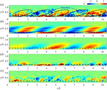
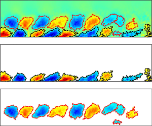
Figure 3(a) illustrates one typical snapshot of  $u(x, y)$ in Case WC. The prominent feature being visualized is the streamwise repetition of outer-scaled
 $u$ structures with alternating signs (indicated by dashed ellipse). These large-scale structures have streamwise coherence over a span of
 $2{\sim} 3\delta$. They are inclined away from the wall, with the tails attaching to the wall and the heads extending into the wake region. It is noted that de Silva et al. (Reference de Silva, Chandran, Hutchins and Marusic2020) observed a similar flow pattern in a TBL measured by multi-camera 2-D planar PIV at
 $Re_\tau =2500$. Based on this observation, they extracted dominant spatial Fourier modes corresponding to superstructures and LSMs. Figure 3(b) shows the dominant Fourier mode corresponding to the snapshot in figure 3(a). The prime spatial pattern, i.e. the streamwise recurrence of large-scale structures that are physically attached to the wall, is well captured. Nevertheless, wall-detached segments in the original snapshot (highlighted by dotted contours in figure 3a) are not evident in the dominant Fourier mode. Figure 3(c–e) illustrates the corresponding reduced-order velocity field, which is contributed by either superstructure-like POD eddies, wall-attached POD eddies or wall-detached POD eddies. These three plots will be revisited in § 4 in the context of POD-based low-order reconstruction.
An example of extracting different components from a snapshot of the instantaneous streamwise fluctuating velocity. (a) The original  $u(x, y)$ in Case WC. Regions highlighted by dashed ellipses or dotted contours denote large-scale coherent motions with quasi-streamwise periodicity or wall-detached clusters, respectively. (b) Dominant spatial Fourier modes of the snapshot in (a). (c–e) Reduced-order velocity field
 $\tilde {u}_{SU}$,
 $\tilde {u}_{AE}$ and
 $\tilde {u}_{DE}$ contributed by superstructure-like POD eddies, wall-attached POD eddies and wall-detached POD eddies, respectively. Horizontal dashed lines in each panel represent the upper bound of the mean-flow log layer.

3.1. Eigenmodes of leading-order POD modes
In the present study, the technique of POD is used for velocity-field decomposition. POD decomposes an ensemble of datasets into discrete modes according to their energy contents. It is the most efficient linear decomposition method to recover the kinetic energy of the original system (Sirovich Reference Sirovich1987; Berkooz, Holmes & Lumley Reference Berkooz, Holmes and Lumley1993). On the other hand, AEH assumes constant energy density within a hierarchy of AEs that are geometrically self-similar with each other (Marusic & Monty Reference Marusic and Monty2019). This leads to the inference that AEs with various length scales are fully separated in their total energy contents. In this sense, the strategy of decomposing velocity fields by energy contents instead of by scales might be practical for the purpose of identifying statistical representations of AEs.
POD has been widely used to extract energetic large-scale features from turbulent flows (Moin & Moser Reference Moin and Moser1991; Duggleby et al. Reference Duggleby, Ball, Paul and Fischer2006; Wu & Christensen Reference Wu and Christensen2010; Wu Reference Wu2014; Hellström et al. Reference Hellström, Ganapathisubramani and Smits2015; Deng et al. Reference Deng, Pan, Wang and He2018). By projecting the spatio-temporal velocity fields onto the subspaces spanned by the POD basis functions, the spatial and temporal behaviour of energy-containing coherent motions can be decoupled. Specifically, the fluctuating velocity fields  $\boldsymbol {V}(\boldsymbol {x},t)$ in a space–time domain of
 $D_{\boldsymbol {X}}\times D_T$ are decomposed into
 $N$ discrete modes
 \begin{equation} \boldsymbol{V}(\boldsymbol{x},t)=\sum_{i=1}^{N}a_i(t) \varPsi_i(\boldsymbol{x}),\end{equation}
in which the spatial eigenmode  $\varPsi _{i}(\boldsymbol {x})$ (also known as the basic function) and the time coefficient
 $a_i(t)$ are orthogonal functions, i.e.
 \begin{equation} \int_{D_{\boldsymbol{X}}}\varPsi_{i}(\boldsymbol{x})\varPsi_{j}(\boldsymbol{x})\,\mathrm{d} \boldsymbol{x}=\delta_{i j}\quad \mbox{and}\quad \int_{D_{T}} a_{i}(t) a_{j}(t)\, \mathrm{d}t=e_{i} \delta_{i j}, \end{equation}
with  $\delta _{i j}$ the Kronecker symbol and
 $e_{i}$ the eigenvalue that measures the relative TKE carried by the
 $i$th mode. POD modes are usually sorted by
 $e_{i}$ in decreasing order. The total number
 $N$ of the mode set is determined by the degree of freedom of
 $\boldsymbol {V}(\boldsymbol {x},t)$. For the purpose of model reduction, a finite number of the first
 $M$ (
 $M< N$) POD modes can be used to reconstruct the reduced-order velocity fields as
 \begin{equation} {\tilde{\boldsymbol{V}}}(\boldsymbol{x},t)=\sum_{i=1}^{M}a_i(t) \varPsi_i(\boldsymbol{x}).\end{equation}
Hereinafter, quantities with  $(\tilde {{\cdot }})$ denote reduced-order fields. For the present TBL datasets, the algorithm of snapshot POD (Berkooz et al. Reference Berkooz, Holmes and Lumley1993) was applied to the whole velocity-field ensemble
 $\boldsymbol {V}(x,y,t)$ (with
 $\boldsymbol {V}=[u\, v]$). Recall that, in Case WC and Case DNS, the streamwise FOV is
 ${\rm \Delta} X=10.6\delta$, while it reduces to
 ${\rm \Delta} X=4.6\delta$ in Case WT. As will be shown in Appendix A, even-order moments of
 $\tilde {u}$ contributed by AE-like turbulent motions, as well as the corresponding streamwise velocity spectra, are insensitive to the size of FOV once
 ${\rm \Delta} X\ge 4.6\delta$. Moreover, the synthetic test in Appendix A will demonstrate the convergence condition of the present POD analysis.
Figure 4(a) plots the  $u$ and
 $v$ components of the spatial eigenmodes, i.e.
 $\varPsi _i^{u}$ and
 $\varPsi _i^{v}$, of the leading-order POD modes of Case WC and Case DNS. Similar topologies are evident in both cases. Specifically,
 $\varPsi _i^{u}$ of the first 7 modes (with
 $i=1, \ldots, 7$), which jointly contribute more than
 $18\,\%$ of the total TKE, are characterized by one layer of streamwise-aligned wall-attached structures with alternating signs. Such a streamwise-recurring topology resembles that of the instantaneous
 $u$ structures shown in figure 3(a), but the typical length scale carried by
 $\varPsi _i^{u}$ is seen to decrease with the increase of the mode rank. Here,
 $\varPsi _i^{v}$ presents scale equivalence and phase coherence with
 $\varPsi _i^{u}$, both of which jointly characterize large-scale Q2 quadrant events (with
 $\varPsi _i^{u}<0$ and
 $\varPsi _i^{v}>0$) and Q4 quadrant events (with
 $\varPsi _i^{u}>0$ and
 $\varPsi _i^{v}<0$) that alternatively appear along the streamwise direction. As for higher-order POD modes, irregularities gradually appear in
 $\varPsi _i^{u \mid v}$ (with
 $i\geq 8$). Specifically, the layer of wall-attached structures in the POD modes become distorted in shape and disordered in size. Meanwhile, additional layers of wall-detached structures appear on the top of wall-attached ones. The phases between these layers are usually unmatched. With the increase of the mode rank, the similarity in
 $\varPsi _i^{u \mid v}$ between Case WC and Case DNS decreases. While for Case WT, due to the smaller streamwise FOV, even
 $\varPsi _i^{u \mid v}$ of the first 7 modes are slightly different from those of Case WC and Case DNS, but the primary topology remains unchanged.
Spatial eigenmodes  $\varPsi ^{u \mid v}_i$ of the first 13 POD modes in Case WC and Case DNS. The left or right column indicate the
 $u$ or
 $v$ component, and the results of Case WC and Case DNS are shown as pseudo-colour map and coloured contours, respectively.

3.2. Scale and energy characteristics of POD modes
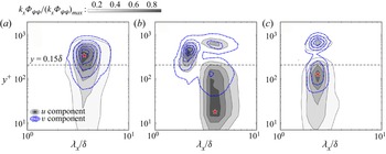
The streamwise periodicity of the leading-order POD eigenmodes can be quantitatively evidenced by figure 5, which plots the pre-multiplied spectrograms, i.e.  $k_x\varPhi _{\varPsi _i^{u} \varPsi _i^{u}}(\lambda _x,y)$ and
 $k_x\varPhi _{\varPsi _i^{v} \varPsi _i^{v}}(\lambda _x,y)$, of three typical POD modes (with
 $i=6, 14, 24$) of Case DNS. Unlike the velocity spectrum (shown in figure 2) that is evaluated among a bulk of velocity-field snapshots, these spectrograms are obtained from only one snapshot of
 $\varPsi _i^{u \mid v}(x,y)$. The insufficient convergence means that they only serve as a qualitative measure of the characteristic length scale of each POD eigenmode. As shown in figure 5, for each leading-order POD mode,
 $k_x\varPhi _{\varPsi _i^{u} \varPsi _i^{u}}$ and
 $k_x\varPhi _{\varPsi _i^{v} \varPsi _i^{v}}$ are rather similar to each other, indicating the scale equivalence between
 $\varPsi _i^{u}$ and
 $\varPsi _i^{v}$. The spectral peak with the peak wavelength
 $\lambda _{x, i}^{peak}$ is always evident. When the mode rank exceeds
 $i=8$, the spectrogram is usually characterized by multiple spectral humps, one in the inner layer and the others in the outer layer (see figure 5(b,c) for instance), consistent with the multi-layer patterns of
 $\varPsi _i^{u}$ (shown in figure 4).
Pre-multiplied streamwise spectrogram  $k_x\varPhi _{\varPsi _i \varPsi _i}(\lambda _x, y)$ of the
 $i$th eigenmode
 $\varPsi ^{u \mid v}_i$ of Case DNS; (a)
 $i=6$, (b)
 $i=14$, (c)
 $i=24$. Red pentagram in each panel indicates the dominant spectral peak.

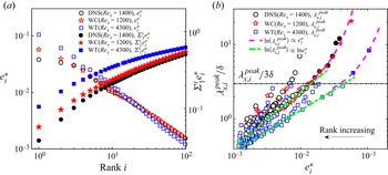
Figure 6(a) plots the relative TKE of each POD mode, which is measured by  $e_{i}^{*}=e_{i} / \sum _{j=1}^{N}e_{j}$, of all three datasets. The cumulative TKE proportion
 $\sum _{j=1}^{i}e_{j}^{*}$ that measures the energy recovery percentage when the first
 $i$ modes are used for low-order reconstruction is also shown. The monotonic descendence of TKE in higher-order POD modes is seen. Notably,
 $e_i^{\ast }$ of Case DNS and Case WC collapse onto each other, except for the first two modes, whose characteristic streamwise length scales are larger than
 $3\delta$ (to be presented later). Such a discrepancy in
 $e_i^{*}$ of the first two POD modes (with
 $i=1,2$) might be attributed to the different tripping conditions in the two cases, which mainly affect large-scale turbulent motions residing in the outer region (Schlatter & Örlü Reference Schlatter and Örlü2012), as can be also seen in figure 8(a). In contrast, the TKE distribution in Case WT is more biased towards lower-order modes. This is consistent with previous observation that, the weight of superstructures in the total TKE is enhanced at higher
 $Re_\tau$ (Balakumar & Adrian Reference Balakumar and Adrian2007).
Energy and scale characteristics of POD modes of all three datasets. (a) The TKE contents  $e_i^{\ast }$ and the cumulative TKE portions
 $\varSigma _1^{i} e_i^{\ast }$ of the first 100 modes. (b) The outer-scaled dominant streamwise wavelength
 $\lambda _{x, i}^{peak}$ with respect to the TKE contents
 $e_i^{\ast }$ of POD modes. Solid symbols in (b) denote superstructure-like POD eddies. Dashed and dash-dotted lines in (b) highlight the main branch of the scale–energy curve, which has the largest
 $e_i^{\ast }$ given a fixed
 $\lambda _{x, i}^{peak}$.

Figure 6(b) plots  $\lambda _{x, i}^{peak}$ of each
 $\varPsi _i^{u}$ as a function of
 $e_i^{\ast }$. For those POD modes that have multiple spectral peaks in
 $k_x\varPhi _{\varPsi _i^{u} \varPsi _i^{u}}$,
 $\lambda _{x, i}^{peak}$ is the wavelength of the one with the largest energy content. It is noted that, due to the limited FOV,
 $\lambda _{x, i}^{peak}$ of the first three POD modes in Case WC and Case DNS, as well as those of the first two modes in Case WT, cannot be accurately measured from
 $k_x\varPhi _{\varPsi _i^{u} \varPsi _i^{u}}$. For all three tested cases, the POD mode scale–energy curves present a pattern of multiple branches, among which the main branch (those highlighted by green and magenta lines in figure 6b) has the largest
 $e_i^{\ast }$ given a fixed
 $\lambda _{x, i}^{peak}$, thus mainly contribute to the total TKE. The main branches of the scale–energy curves in Case WC and Case DNS roughly collapse onto each other, both present an power-law scaling of
 $\ln (\lambda _{x, i}^{peak}) \propto \ln (e_i^{\ast })$ in the range of
 $\lambda _{x, i}^{peak}<3\delta$ and an exponential scaling of
 $\ln (\lambda _{x, i}^{peak})\propto e_i^{*}$ when
 $\lambda _{x, i}^{peak}>3\delta$. Such a dual-scaling behaviour is also evident in the curve of Case WT, which is right shifted from the two low-
 $Re$ curves due to the increased TKE content of larger-scale turbulent motions at higher
 $Re$ (Hutchins & Marusic Reference Hutchins and Marusic2007). In the following, we will interpret structures in POD modes as POD eddies. The monotonic trend of the main branch of the scale–energy curve (in figure 6b) suggests the consistency between scale hierarchy and energy hierarchy of energy-bearing POD eddies, i.e. smaller POD eddies (usually with higher-order POD rank), contains less energy in total. Noting that AEH assumes constant energy density in AEs with various scales, this is not in conflict with the energy hierarchy observed here, since
 $e_i^{\ast }$ measured here is the total TKE contributed by a set of POD eddies with equivalent scales being integrated within the whole FOV.
Superstructures are commonly accepted to have a streamwise length scale of  $\lambda _{x}\ge 3\delta$ (Balakumar & Adrian Reference Balakumar and Adrian2007). Such a length scale range is met by the first seven modes in Case WC and Case DNS and the first two modes in Case WT. As has been shown in the above, these leading-order modes all present a topology of one layer of wall-attached structures; the scaling of their characteristic length scales with respect to the TKE contents is different to that of high-order modes. Therefore, they are inferred to be the statistical representations of superstructures, and are denoted as superstructure-like modes in the following. It is noted that some higher-order modes not residing in the main branch of the scale–energy curves (shown in figure 6b) also satisfy the condition of
 $\lambda _{x, i}^{peak}>3\delta$. They are deemed as being contaminated by the footprint of the leading-order POD modes due to the inevitable POD mode mixing problem (Wang et al. Reference Wang, Pan and Wang2019b). This can be seen in figure 5(b), in which the near-wall spectral patch in
 $k_x\varPhi _{\varPsi _i^{u} \varPsi _i^{u}}$ of the
 $14$th POD mode might be the remnant of that of the
 $6$th POD mode shown in figure 5(a). Based on this observation, those wall-attached parts in higher-order POD modes with streamwise length scale larger than
 $3\delta$ (
 $\lambda _x^{peak}>3\delta$) are also included in the subset of superstructure-like modes.
3.3. Statistical properties of POD eddies
Referring to the multi-layer topology of non-superstructure-like POD eigenmodes, it is natural to ask whether or not the first-layer ‘wall-attached’ structures in the eigenmodes are the statistical representations of AEs. Recalling that several studies have treated wall-attached patterns in POD eigenmodes as AEs (Wu Reference Wu2014; Hellström et al. Reference Hellström, Ganapathisubramani and Smits2015, Reference Hellström, Marusic and Smits2016), we would like to review such a viewpoint by threefold considerations. Firstly, structures in POD eigenmodes  $\varPsi _i$ can be treated as statistical eddies, since they embody the spatio-temporal coherence embedded in turbulent motions. In this sense, these structures are termed as POD eddies. Secondly, the existence of ‘wall-attached’ POD eddies provides a sufficient but not necessary condition for the existence of wall-attached physical structures. Thirdly, the orthogonality of POD modes makes each POD eddy independently contribute to the total TKE. The latter two aspects are further explained as follows.
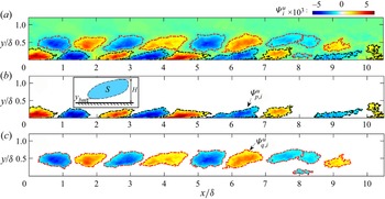
Based on the first consideration, for the  $i$th POD mode, the
 $u$ component eigenmode
 $\varPsi _i^{u}$ (as illustrated in figure 7(a) with
 $i=24$) can be decomposed into discrete POD eddies
 $\varPsi _{p, i}^{u}$. Using the criterion that will be described later,
 $\varPsi _{p, i}^{u}$ can be further divided into a ‘wall-attached’ subset
 $\varPsi _{i}^{u, {AE}}$ (as shown in figure 7b) and a ‘wall-detached’ subset
 $\varPsi _{i}^{u, {DE}}$ (as shown in figure 7c). This forms a decomposition of
 $\varPsi _i^{u}$ as
 \begin{equation} \varPsi_{i}^{u}(x,y)=\varPsi_{i}^{{AE}}(x,y)+\varPsi_{i}^{{DE}}(x,y) +\varPsi_{i}^{{res}}(x, y),\end{equation}
in which  $\varPsi _{i}^{res}$ is the residual component, whose magnitude is almost one order smaller than those of
 $\varPsi _{i}^{AE}$ and
 $\varPsi _{i}^{DE}$. Hereinafter, only
 $u$ component eigenmodes are discussed; therefore, the subscript
 $u$ in
 $\varPsi _i^{u}$ is not explicitly shown for convenience. The superscripts (or subscripts) AE and DE denote that the related quantity is contributed by wall-attached eddies and wall-detached eddies, respectively.
Illustration of the procedure of decomposing the eigenmode  $\varPsi _{i}$ into wall-attached and wall-detached POD eddies. (a–c) Show the original
 $u$ component
 $\varPsi _{i}$, wall-attached part
 $\varPsi ^{{AE}}_{i}$ and wall-detached part
 $\varPsi ^{{DE}}_{i}$ of the
 $24$th POD mode in Case DNS, respectively. Contour lines denote the level of
 $\alpha \varPsi _i^{max}$ or
 $\alpha \varPsi _i^{min}$ with
 $\alpha =0.2$. The inset in (b) defines the height
 $H$, the area
 $S$ and the lowest position
 $y_{bm}$ of one single POD eddy.

Any two POD eddies in one POD mode are fully separated from each other, i.e.
 \begin{equation} \varPsi_{p, i}(x,y) \varPsi_{q, i}(x,y)=0,\quad p \neq q,\end{equation}
in which  $\varPsi _{p, i}$ and
 $\varPsi _{q, i}$ are two non-overlapping structures (as illustrated in figure 7), i.e.
 \begin{equation} \varPsi_{i}^{{AE}}(x,y)\varPsi_{i}^{{DE}}(x,y)=0.\end{equation}
Such a non-overlapping condition incorporates the idea of ‘spatial exclusion’ in de Silva et al. (Reference de Silva, Woodcock, Hutchins and Marusic2016b). Namely, the representative eddies of the same hierarchical scale are totally separated from each other in space. It is noted that (3.6) cannot be applied to POD eddies in different modes.
The second consideration stated above deals with the relationship between wall-attached POD eddies and wall-attached physical structures. It can be conceptually explained as follows. Hwang & Sung (Reference Hwang and Sung2018) regarded a hierarchy of instantaneous velocity clusters that are physically ‘attached’ to the wall as the representations of AEs. On the other hand, instantaneous reduced-order velocity structures can be reconstructed by a linear combination of selected POD modes via (3.3). In this context, let us suppose an extreme scenario of one wall-attached POD eddy  $\varPsi _{p, i}^{AE}$ in mode
 $i$ and one wall-detached POD eddy
 $\varPsi _{q, j}^{DE}$ in mode
 $j$. If
 $i=j$,
 $\varPsi _{p, i}^{AE}$ and
 $\varPsi _{q, j}^{DE}$ are spatially separated from each other via (3.5). If
 $i \neq j$, for the reduced-order velocity field
 $\tilde {u}(x,y,t)$ reconstructed by
 $\varPsi _{p, i}^{AE}$ and
 $\varPsi _{q, j}^{DE}$ via (3.3), given a time instant
 $t$ that is dominated by mode
 $i$ (with dominant time coefficient
 $a_i(t)\ge a_j(t)$), the signature of
 $\varPsi _{p, i}^{AE}$ in
 $\tilde {u}(x,y,t)$ cannot be completely masked by that of
 $\varPsi _{q, j}^{DE}$. In this sense, a wall-attached part will be evident in
 $\tilde {u}(x,y,t)$. Another scenario is two wall-attached POD eddies in different modes that possess opposite spatio-temporal phases. Owing to the scale hierarchy, it is unlikely for them to completely cancel each other in
 $\tilde {u}(x,y,t)$. Based on these two arguments, wall-attached POD eddies are regarded as the projection of wall-attached velocity structures onto the subspace spanned by POD modes; namely, they have physical significance.
The third consideration, i.e. the independent TKE contribution of POD eddies, can be formulated by decomposing the  $u$ component TKE, i.e.
 $\langle u^{2} \rangle$, as
 \begin{align} \langle u^{2}(y)\rangle &=\frac{1}{{\rm \Delta} X} \frac{1}{{\rm \Delta} T} \int_{x} \int_{t}\left[\sum_{i}^{N} a_{i}(t) \varPsi_{i}(x,y)\right]^{2} \, \mathrm{d}t\, \mathrm{d} x \nonumber\\ &=\underbrace{\sum_{i}^{N}\left[\frac{1}{{\rm \Delta} T} \int_{t} a_{i}^{2}(t)\, \mathrm{d}t \frac{1}{{\rm \Delta} X} \int_{x} \varPsi_{i}^{2}(x,y)\, \mathrm{d} x\right]}_{\text{term I}}\nonumber\\ &\quad + \underbrace{\sum_{i}^{N} \sum_{j}^{N}\left[\frac{1}{{\rm \Delta} T} \int_{t} a_{i}(t) a_{j}(t)\, \mathrm{d}t \frac{1}{{\rm \Delta} X} \int_{x} \varPsi_{i}(x,y) \varPsi_{j}(x,y) \, \mathrm{d} x\right]_{i\neq j}}_{\text{term II}=0}. \end{align}
According to the orthogonality condition of (3.2a,b), term II on the right-hand side of (3.7), which is related to the interaction between different POD modes, is zero. Using (3.2a,b) and (3.5) and (3.6) and ignoring the residual component  $\varPsi _i^{res}$ for a leading-order approximation,
 $\langle u^{2} \rangle$ can be further expanded as
 \begin{align} \langle u^{2}(y)\rangle
&=\sum_{i}^{N}\left\{\frac{1}{{\rm \Delta} T} \int_{t}
a_{i}^{2}(t)\, \mathrm{d}t \frac{1}{{\rm \Delta} X}
\int_{x}[\varPsi_{i}^{AE}(x, y)+\varPsi_{i}^{DE}(x, y)]^{2}
\, \mathrm{d} x\right\} \nonumber\\ &=\sum_{i}^{N}
\frac{1}{{\rm \Delta} T} e_{i} \frac{1}{{\rm \Delta} X}
\int_{x}\left\{\underbrace{[\varPsi_{i}^{AE}(x,
y)]^{2}}_{\text{attached
component}}+\underbrace{[\varPsi_{i}^{DE}(x, y)
]^{2}}_{\text{detached component }}+\underbrace{2
\varPsi_{i}^{AE}(x, y) \varPsi_{i}^{DE}(x, y)}_{\text{cross
term}= 0} \right\}\,\mathrm{d} x \nonumber\\
&=\underbrace{\sum_{i}^{N} \sum_{p}^{P_{i}}
\left\{\frac{1}{{\rm \Delta} T} \frac{1}{{\rm \Delta} X} e_{i}
\int_{x}[\varPsi_{p, i}^{AE}(x, y)]^{2}\, \mathrm{d}
x\right\}}_{\text{attached component}}+
\underbrace{\sum_{i}^{N} \sum_{q}^{Q_{i}}
\left\{\frac{1}{{\rm \Delta} T} \frac{1}{{\rm \Delta} X} e_{i}
\int_{x}[\varPsi_{q, i}^{DE}(x, y)]^{2} \, \mathrm{d}
x\right\}}_{\text{detached component}}.
\end{align}
Due to the non-overlapping condition of (3.6), the cross-term in the second line of (3.8) is always zero. The last line of (3.8) clearly indicates that the total TKE is independently contributed by individual POD eddies, i.e.  $\varPsi _{p, i}^{AE}$ and
 $\varPsi _{q, i}^{DE}$.
Considering the properties of physical significance, statistical independence, as well as scale hierarchy of wall-attached POD eddies, it is reasonable to treat them as candidates for statistical representations of AEs. Before demonstrating that these statistical structures well restore most of the kinematic characteristics predicted by AEH, it is necessary to accurately separate them from wall-detached POD eddies. This issue will be addressed in the next subsection.
3.4. Criterion for wall-attached POD eddies
The clustering method proposed by Hwang & Sung (Reference Hwang and Sung2018) for the detection of instantaneous wall-attached velocity structures is used here with slight modification to isolate wall-attached and wall-detached POD eddies from POD eigenmodes. Taking  $\varPsi _i(x,y)$ with
 $i=24$ in Case DNS (shown in figure 7a) as an example, the procedure has four steps, i.e.
(i) Find the maximum and minimum value, i.e.
 $\varPsi _i^{max}$ and $\varPsi _i^{min}$, in $\varPsi _i(x,y)$.
(ii) Binarize
$\varPsi _i(x,y)$ into a set of cluster regions with a threshold of $\varPsi _i(x,y)>\alpha \varPsi _i^{max}$ for positive clusters or $\varPsi _i(x,y)<\alpha \varPsi _i^{min}$ for negative clusters.(iii) Calculate the geometric parameters of each cluster region, including the area
$S$, the height $H$ and the lowest position $y_{bm}$, whose definitions are illustrated in figure 7(b).(iv) Categorize cluster regions by the wall-attachment condition. Namely, those cluster regions with
$S>S_t$, $H>H_t$ and $y_{bm}< y_{t}$ (or $y_{bm}\geq y_{t}$) are accepted as wall-attached (or wall-detached) POD eddies, as shown in figure 7(b) (or figure 7c).


In this method, the threshold for the minimum height is set as  $H^{+}_{t}=100$ for consistency with previous work (Perry & Chong Reference Perry and Chong1982; Baars & Marusic Reference Baars and Marusic2020a; Hu et al. Reference Hu, Yang and Zheng2020). The area threshold is set to
 $S^{+}_{t}=1600$, slightly larger than the average area of small-scale vortices (Wu & Christensen Reference Wu and Christensen2006; Herpin et al. Reference Herpin, Stanislas, Foucaut and Coudert2013). According to a percolation test (not shown here for brevity), the strength threshold is set to
 $\alpha =0.2$, around which the yielded AE-like kinematics are found to be insensitive to
 $\alpha$. The wall-attachment threshold is
 $y^{+}_{t}=60$, which is a loose criterion if comparing with the previously used thresholds of
 $y^{+}_{t}=15$ in Baars et al. (Reference Baars, Hutchins and Marusic2017) and
 $y^{+}_{t}=20$ in Hwang & Lee (Reference Hwang and Lee2020a). Such a choice is to adapt to the experimental dataset, in which the flow region below
 $y^{+}=25$ cannot be faithfully accessed by the present large-FOV PIV measurement. The side effect is that those wall-attached POD eddies that have weak spatial coherence down to the wall can be preserved. In Appendix B, the threshold of
 $y^{+}_{t}=15$ is applied to Case DNS to test the effect of the wall-attachment condition.
The present clustering method is different to that of Hwang & Sung (Reference Hwang and Sung2018) in two aspects. Firstly, since eigenmodes themselves are non-dimensional, the extreme value ( $\varPsi _i^{max}$ and
 $\varPsi _i^{min}$) in the whole eigenmode, rather than the local measure of velocity fluctuating intensity that varies along
 $y$ (Hwang & Sung Reference Hwang and Sung2018), is used as the global strength measure for binarization. Secondly, due to the 2-D nature of the dataset, the connectivity is evaluated in a 2-D scenario. Considering the statistical independency of POD modes that has been addressed in § 3.3, 2-D connectivity is enough to guarantee that wall-attached POD eddies statistically represent the 2-D projection of physical structures that are ‘attached’ to the wall.
Using this clustering method, all of the POD modes can be decomposed into four subsets, i.e. superstructure-like POD eddies, wall-attached POD eddies, wall-detached POD eddies and small-scale motions. As has been stated in § 3.2, those near-wall POD eddies associated with the footprints of superstructures (with streamwise length  $\lambda _x^{peak}>3\delta$) are sorted into the subset of superstructure-like modes. Wall-attached or wall-detached POD eddies have characteristic streamwise scales ranging from
 $O(40l^{*})$ to
 $3\delta$. Meanwhile, small-scale motions compose POD eddies whose area (or length scale) is smaller than
 $1600l^{*2}$ (or
 $40l^{*}$), as well as residual components in each POD mode. The kinematic statistics of these four subsets will be analysed in the next section.
4. Kinematic statistics of various POD eddies
In this section, reduced-order reconstruction similar to (3.3) is applied to the above decomposed four subsets of POD eddies. The yielded quantities are denoted by the subscript  ${SU}$,
 ${AE}$,
 ${DE}$ and
 ${SS}$, respectively. Figure 3(c–e) illustrates
 $\tilde {u}_{{SU}}(x,y)$,
 $\tilde {u}_{{AE}}(x,y)$ and
 $\tilde {u}_{{SS}}(x,y)$ corresponding to the original snapshot shown in figure 3(a). It is clearly seen that instantaneous structures that are physically attached to or detached from the wall are captured by
 $\tilde {u}_{{AE}}$ or
 $\tilde {u}_{{DE}}$, respectively. Meanwhile, the streamwise reoccurring pattern of large-scale structures in the original snapshot is mainly carried by
 $\tilde {u}_{{SU}}$. The kinematic statistics of these reduced-order components are to be analysed in the following. The main concern is to see whether or not wall-attached POD eddies present kinematic scaling predicted by AEH.
4.1. Log law of the second-order moments
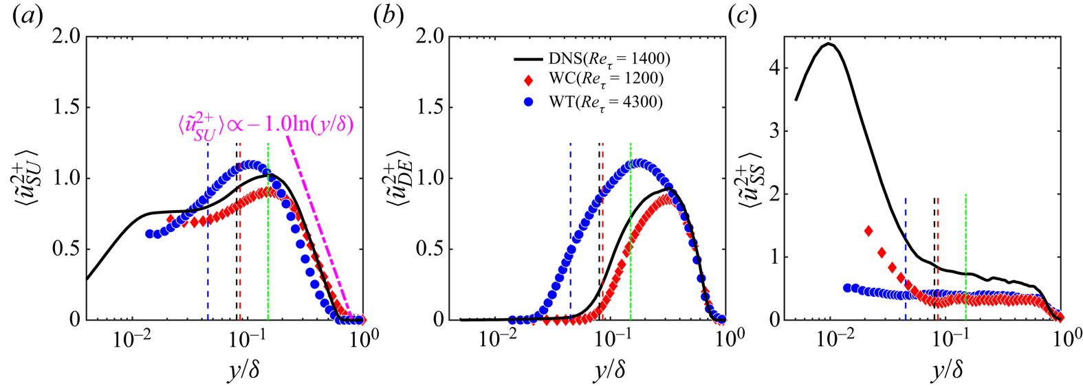
Figures 8 and 9 show the wall-normal profiles of the fluctuation intensity  $\langle \tilde {u}_\chi ^{2}\rangle$ contributed by each subset of POD modes (
 $\chi ={SU, AE, DE, SS}$) in all three datasets. As shown in figure 8(a),
 $\langle \tilde {u}_{SU}^{2}\rangle$ is non-negligible in the near-wall region and reaches a peak value close to the upper bound of the log layer. The inner-layer parts of
 $\langle \tilde {u}_{SU}^{2} \rangle (y)$ in Case WC and Case DNS have similar shape but are vertically shifted from each other by a constant. This might be attributed to the different tripping conditions that mainly affect large-scale turbulent motions residing in the outer region (Schlatter & Örlü Reference Schlatter and Örlü2012). On the other hand, the profiles of
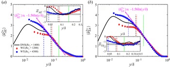
 $\langle \tilde {u}_{AE}^{2+}\rangle (y)$ (shown in figure 9a) of all three cases are seen to collapse onto each other in the lower bound of the log layer and above. Such a
 $Re$-independency suggests that wall-attached POD eddies are fully resolved by the present PIV measurements. In § 5, the profiles of the even-order moment of
 $\tilde {u}_{AE}(y)$ of Case WC and Case WT are seen to overlap in the mean-flow log layer. This provides another evidence for the consideration that the different tripping conditions do not affect kinematics of wall-attached POD eddies.
Wall-normal profiles of the streamwise TKE contributed by (a) superstructure-like POD eddies, (b) wall-detached POD eddies and (c) small-scale motions. Vertical dashed lines or dash-dotted lines indicate the lower or the upper bound of the mean-flow log layer in the same sense as those shown in figure 1(b).

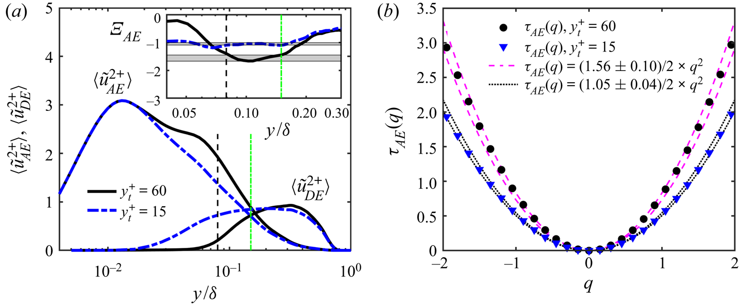
Wall-normal profiles of the streamwise TKE contributed by (a) wall-attached POD eddies and (b) wall-attached POD eddies together with superstructure-like POD eddies. Vertical dashed lines or dash-dotted lines indicate the lower or the upper bound of the mean-flow log layer in the same sense as those shown in figure 1(b). Insets in (a) and (b) respectively plot the logarithmic indicator functions  $\varXi _{AE}$ and
 $\varXi _{SA}$ defined in (4.3), the horizontal grey patches indicate the Townsend–Perry constant of
 $A^{AE}_1=1.56\pm 0.10$.

In figure 8(c),  $\langle \tilde {u}_{SS}^{2}\rangle$ of Case DNS peaks at approximately
 $y^{+}=15$, its magnitude becomes rather weak in the outer layer. Since these small-scale motions cannot be fully resolved in the present PIV measurement due to the insufficient spatial resolution, there is an overall underestimation of
 $\langle \tilde {u}_{SS}^{2}\rangle$ in Case WC and Case WT. As for wall-detached POD eddies, figure 8(b) shows that
 $\langle \tilde {u}_{DE}^{2}\rangle$ is negligible in the near-wall region due to the wall-detachment condition and reaches a peak outside the mean-flow log layer.
According to AEH, the wall-normal profile of  $\langle u^{2+}\rangle$ at asymptotically high
 $Re$ presents a logarithmic law in the mean-flow log layer, i.e.
 \begin{equation} \langle u^{2+}\rangle=B_1-A_1\ln (y/\delta).\end{equation}
In the present study, due to the low-to-moderate  $Re$, the logarithmic law is not prominent in full-order profile of
 $\langle u^{2}\rangle$(y) (as shown in figure 1b). In contrast, figure 9(a) shows that the profile of
 $\langle \tilde {u}_{AE}^{2}\rangle (y)$ contributed by wall-attached POD eddies presents a distinct logarithmic decay in the mean-flow log layer, i.e.
 \begin{equation} \langle \tilde{u}_{AE}^{2+}\rangle=B^{AE}_1-A^{AE}_1\ln (y/\delta).\end{equation}
For a quantification of (4.2), the logarithmic indicator function, i.e.
 \begin{equation} \varXi_{AE}(y)=y\partial\langle \tilde{u}_{AE}^{2+}\rangle/\partial y,\end{equation}
which is the slope of  $\langle \tilde {u}_{AE}^{2}\rangle (y)$ in a semi-logarithmic plot, is examined. The inset in figure 9(a) shows that
 $\varXi _{AE}$ in all three cases remains constant throughout the mean-flow log layer. The Townsend–Perry constant, which can be determined from the constant part of
 $\varXi _{AE}(y)$, is
 $A^{AE}_1=1.56\pm 0.10$ for all three cases. This value is higher than those reported by Baars & Marusic (Reference Baars and Marusic2020b) (
 $A^{AE}_1=0.98$), Hu et al. (Reference Hu, Yang and Zheng2020) (
 $A^{AE}_1=1.0$) and Hwang & Lee (Reference Hwang and Lee2020a) (
 $A^{AE}_1=0.37$). As will be shown in Appendix B, when the wall-attachment condition of
 $y_t^{+}=15$ is chosen, the magnitude of
 $A^{AE}_1$ of Case DNS reduces to
 $1.05\pm 0.04$. Such a dependence of
 $A^{AE}_1$ on
 $y_t^{+}$ will be further explained in Appendix B.
Figure 9(b) plots  $\langle \tilde {u}_{SA}^{2+}\rangle$ contributed by both superstructure-like and wall-attached POD eddies in a similar way. Here, the subscript
 ${SA}$ is the abbreviation of ‘
 ${SU+AE}$’. The logarithmic scaling is still evident, but the log-law regions of all three profiles are shifted outwards from
 $3\sqrt {Re_\tau }< y^{+}<0.15\delta ^{+}$ to
 $0.1\delta < y<0.3\delta$. This observation is in line with Meneveau & Marusic (Reference Meneveau and Marusic2013), who reported a log law of
 $\langle u^{2}\rangle (y)$ in the region of
 $400< y^{+}<0.3\delta ^{+}$ when
 $Re_\tau =2800 {\sim} 19\ 000$.
According to AEH, the log law of  $\langle u^{2} \rangle (y)$ is contributed by a hierarchy of self-similar AEs. Hwang & Sung (Reference Hwang and Sung2018) successfully exemplified this conceptual picture by hierarchically superimposing instantaneous wall-attached
 $u$ structures with various scales. Based on the general consistency between the scale hierarchy and the energy ranking of POD modes that has been shown in § 3.2, it is natural to ask whether or not the log law can be restored by a hierarchy of wall-attached POD eddies. Referring to (3.8), this consideration can be examined by integrating the TKE contribution of each rank of POD eddies in a hierarchical sense. Figure 10 shows the wall-normal profiles of
 $\varSigma ^{\infty }_i\langle \tilde {u}^{2+}_{{AE}, i}\rangle$ of all three cases, in which leading-order POD modes with mode rank smaller than
 $i$ are gradually knocked out of the integration. The purpose is to quantify the condition for the appearance of the AE-contributed log-law scaling of (4.2). It is noted that superstructure-like POD eddies are excluded from the integration of
 $\varSigma ^{\infty }_i\langle \tilde {u}^{2+}_{{AE}, i}\rangle$.
Wall-normal profiles of the streamwise TKE contributed by wall-attached POD eddies in all  $j$ POD modes with
 $j\ge i$, i.e.
 $\varSigma ^{\infty }_i \langle \tilde {u}^{2+}_{{AE}, i} \rangle$. (a) Case DNS and WC; (b) Case DNS and WT. Vertical dashed lines or dash-dotted lines indicate the lower or the upper bound of the mean-flow log layer in the same sense as those shown in figure 1(b).

As show in figure 10, for all three cases, the logarithmic behaviour would appear only if enough energy hierarchies (or mode ranks) are included. Taking Case WT as an example (shown in figure 10b), knocking out the first  $79$ POD modes (with
 $\lambda _{x, i}^{peak}>0.5\delta$) from the integration of
 $\varSigma ^{\infty }_i\langle \tilde {u}^{2+}_{{AE}, i}\rangle$ only lowers the overall level of the curve and shifts the log-law region towards the wall. When further increasing the lower integration limit to
 $i=300$ (with
 $\lambda _{x, i}^{peak}=0.2\delta$), the slope of the log-law scaling is remarkably smaller than
 $A^{AE}_1=1.56$. A similar observation is also seen in Case WC and Case DNS. The difference is that, due to the insufficient scale separation, the minimum mode rank for the appearance of the log-law slope of
 $A^{AE}_1=1.56$ reduces to
 $i=15$ (with
 $\lambda _{x, i}^{peak}=2\delta$). Such an observation suggests that small-scale wall-attached POD eddies may not pose a kinematic self-similarity that is the same to those of large-scale ones.
4.2. Streamwise velocity spectrum
By incorporating the statistical and structural perspective as a whole, Baars et al. (Reference Baars, Hutchins and Marusic2017) proposed a linear coherent spectrum (LCS) method to show that the signature of AE-like turbulent motions in the streamwise velocity spectrum was encompassed by a spectral triangle of
 \begin{equation} y^{+}> 80, \lambda_x>14y, \lambda_x< 10\delta.\end{equation}
On the other hand, Hu et al. (Reference Hu, Yang and Zheng2020) proposed another spectral triangle, i.e.
 \begin{equation} y^{+}> 100, \lambda_x>5.7y, \lambda_x< 3\delta,\end{equation}
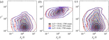
based on spectral scaling arguments. Referring to figure 2(a), these two spectral triangles are only partly evident in the pre-multiplied streamwise spectrogram  $k_x\varPhi _{uu}(\lambda _x, y)$ of Case WT. Figures 11 and 12 plot the pre-multiplied streamwise spectrograms of
 $\tilde {u}$ that are reconstructed by wall-attached POD eddies, wall-detached POD eddies or both of them for all three tested cases. Hereinafter, they are denoted as
 $k_x\varPhi _{\chi }$ with
 $\chi =\{{AE, DE, AD}\}$ (with AD short for ‘
 ${AE+DE}$’). The purpose is to see which subset of POD modes contribute to these spectral triangles.
Pre-multiplied streamwise spectra of  $\tilde {u}$ contributed by (a) wall-attached POD eddies, (b) wall-detached POD eddies and (c) both of them. Here,
 $y_t^{+}=60$. Grey scale patches with thin solid contours in black denote results of Case DNS and bold dash-dotted contours in red correspond to Case WC. The spectra are normalized by their maximum value beyond
 $y^{+}=40$. The iso-contours are plotted at the level of 0.15 : 0.15 : 1.2. The magenta dash-doted and black solid triangles indicate the spectral triangle of (4.4) and (4.5), respectively.

Pre-multiplied streamwise spectra of  $\tilde {u}$ contributed by (a) wall-attached POD eddies, (b) wall-detached POD eddies and (c) both of them in Case WT. Here,
 $y_t^{+}=60$. The format is the same as that in figure 11.

As shown in figures 11 and 12, the hypotenuse of the spectral contour of  $k_x\varPhi _{AE}$ of wall-attached POD eddies presents a scaling of
 $\lambda _x \propto y^{\beta _1}$ in the range of
 $0.2\delta <\lambda _x<3\delta$, with
 $\beta _1=2$ in Case WC and Case DNS and
 $\beta _1=1.5$ in Case WT. While
 $k_x\varPhi _{DE}$ of wall-detached POD eddies presents an inclined elliptical shape, the spectral peak is located outside the spectral triangle of (4.5), and the ridge line across it roughly follows a scaling of
 $\lambda _x \propto y^{\beta _2}$ with
 $\beta _2=1.8$ in Case WC and Case DNS and
 $\beta _1=1.5$ in Case WT. As for
 $k_x\varPhi _{AD}$, which according to (3.8) is the sum of
 $k_x\varPhi _{DE}$ and
 $k_x\varPhi _{AE}$, its energetic part is mainly encompassed by (4.5). This evidences that the spectral triangle of Hu et al. (Reference Hu, Yang and Zheng2020) cannot be regarded as a spectral signature, being only contributed to by wall-attached motions. By contrast, (4.4) only encompass the large-scale part of
 $k_x\varPhi _{AE}$. It is consistent with the fact that such a spectral triangle is obtained by a novel LCS method that detects LSMs with strong coherence down to the near-wall region (Baars et al. Reference Baars, Hutchins and Marusic2017).
Additionally, figure 22 in Appendix B will show that, when the wall-attachment condition is set to  $y_t^{+}=15$, for Case DNS, the hypotenuse in
 $k_x\varPhi _{AE}$ follows a linear scaling of
 $\lambda _x \propto y$. This is consistent with Baars & Marusic (Reference Baars and Marusic2020a,Reference Baars and Marusicb), who observed the self-similar scaling of wall-attached motions (with the wall-reference height
 $y_t^{+}=15$) in a wide range of
 $Re_\tau$. Therefore, it is felt that the strict wall-attachment condition is a necessary for the appearance of the self-similarity in the spectral of wall-attached POD eddies.
5. Quasi-Gaussian behaviour of wall-attached and wall-detached POD eddies
Another property that has been assumed in AEH is the Gaussian behaviour of AE-like turbulent motions. It states that AEs randomly appear in spatio-temporal space, and their kinematics and dynamics are independent of each other. The Gaussian assumption was invoked by Meneveau & Marusic (Reference Meneveau and Marusic2013) to predict the existence of a generalized logarithmic scaling of high-even-order moments of full-order  $u$. de Silva et al. (Reference de Silva, Marusic, Woodcock and Meneveau2015) and Yang, Marusic & Meneveau (Reference Yang, Marusic and Meneveau2016) further used this assumption to formulate the log-law scaling of the longitudinal SFs of
 $u$ and the power-law scaling of the MGF, respectively. Cheng et al. (Reference Cheng, Li, Lozano-Durán and Liu2020) and Hu et al. (Reference Hu, Yang and Zheng2020) recently provided new insights into the log-law scaling of high-even-order moments of AE-like turbulent motions, which were isolated from full-order velocity fields via either a structure-identification approach or a spectral decomposition method. Following these studies, the scaling behaviour of high-even-order moments of
 $\tilde {u}_{AE}$, as well as their longitudinal SF and MGF, are analysed in this section. Note that datasets in the whole
 $x$ span of the FOV were used to guarantee the statistical convergence of these quantities. Since the quasi-Gaussian behaviours of Case DNS and Case WC are quite similar, only results for Case WC and Case WT are presented in this section for brevity.
5.1. Log law of high-even-order moments
According to Meneveau & Marusic (Reference Meneveau and Marusic2013), if AEs are statistically independent in energy contributions and are randomly distributed in spatio-temporal space, a generalized log law of high-even-order moments of  $u$, i.e.
 \begin{equation} \langle u^{2p+}\rangle^{1/p}=B_p-A_p\ln (y/\delta),\end{equation}
can be deduced within the framework of AEH. By invoking the central limit theorem, the log-law slope  $A_p$ in (5.1) follows
 \begin{equation} A_p=A_1[(2p-1)!!]^{1/p},\end{equation}
in which  $n!!\equiv n(n-2)(n-4) \ldots 1$ is the double factorial and
 $A_1$ is the Townsend–Perry constant. Several studies (de Silva et al. Reference de Silva, Marusic, Woodcock and Meneveau2015; Woodcock & Marusic Reference Woodcock and Marusic2015; Cheng et al. Reference Cheng, Li, Lozano-Durán and Liu2020; Hu et al. Reference Hu, Yang and Zheng2020) have confirmed the existence of the generalized log law of (5.1) in the inertial layer. But
 $A_p$ were found to be lower than the prediction of (5.2), thus implying a sub-Gaussian behaviour.
Figure 13(b) shows the wall-normal profiles of  $\langle \tilde {u}_{AE}^{2p}\rangle ^{1/p}$ (with
 $p=1, \ldots, 5$) that are contributed by wall-attached POD eddies in Case WC and Case WT. The profiles of full-order velocity fields, i.e.
 $\langle \tilde {u}^{2p}\rangle ^{1/p}$, as well as those contributed by both wall-attached POD eddies and superstructure-like POD eddies, i.e.
 $\langle \tilde {u}_{SA}^{2p}\rangle ^{1/p}$, are plotted in figures 13(a) and 13(c) for comparison. Due to the insufficient
 $Re$, it is not
 $\langle u^{2p}\rangle ^{1/p}$ but
 $\langle \tilde {u}_{AE}^{2p}\rangle ^{1/p}$ that presents a distinct logarithmic decay in the mean-flow log layer until
 $p=5$. When superstructure-like POD eddies are included, the log law in
 $\langle \tilde {u}_{SA}^{2p}\rangle ^{1/p}(y)$ still exists, but the upper bound of the log-law region shifts outwards from
 $0.15\delta$ to approximately
 $0.3\delta$. Note that Meneveau & Marusic (Reference Meneveau and Marusic2013) have reported a similar outward shift of the log-law region of full-order
 $\langle u^{2p}\rangle ^{1/p}(y)$ in the high
 $Re$ regime. Furthermore, the log law is distorted when the contributions from wall-detached POD eddies are taken into account (not shown for simplicity). All these observations hold for the three tested cases.
High-even-order moments of (a)  $u$, (b)
 $\tilde {u}_{AE}$ and (c)
 $\tilde {u}_{SA}$ as a function of
 $y/\delta$. Vertical dashed lines or dash-dotted lines indicate the lower or the upper bound of the mean-flow log layer in the same sense as those shown in figure 1(b).

The log–linear slopes  $A^{AE}_p$ estimated from the
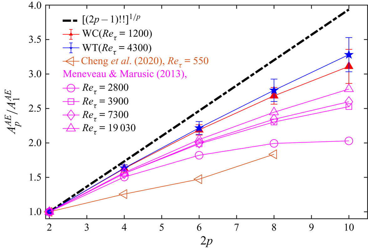
 $\langle \tilde {u}_{AE}^{2p}\rangle ^{1/p}(y)$ profiles are further plotted in figure 14. Those value reported in Meneveau & Marusic (Reference Meneveau and Marusic2013) and Cheng et al. (Reference Cheng, Li, Lozano-Durán and Liu2020) are also shown. Although
 $A^{AE}_p$ in the present study are closer to the Gaussian baseline than those in the literatures, they are still sub-Gaussian. This observation is supported by the study of de Silva et al. (Reference de Silva, Woodcock, Hutchins and Marusic2016b), who found that, when AEs in the same scale hierarchy were totally spatially excluded (without spatial overlap), a sub-Gaussian behaviour of their streamwise higher-order moments could be expected.
The log–linear slopes  $A^{AE}_p$ of the logarithmic part of
 $\langle \tilde {u}_{AE}^{2p}\rangle ^{1/p}(y)$. The error bars are the standard deviation of
 $A^{AE}_p$ when changing the fitting region in the mean-flow log layer. The results of Meneveau & Marusic (Reference Meneveau and Marusic2013) and Cheng et al. (Reference Cheng, Li, Lozano-Durán and Liu2020) are plotted as hollow symbols for reference.

5.2. Moment-generating function
By invoking AEH in together with the Gaussian assumption of inertial motions, Yang et al. (Reference Yang, Marusic and Meneveau2016) derived a power-law scaling of the single-point MGF of  $u$, i.e.
 \begin{equation} \langle \exp (qu^{+})\rangle=(y/\delta)^{-\tau(q)},\end{equation}
where  $\langle \exp (qu^{+})\rangle$ is the MGF of
 $u$ dialled by a real number
 $q$. The larger
 $q$ the larger weight of high-magnitude
 $u$ in
 $\langle \exp (qu^{+})\rangle$. The scaling factor
 $\tau$ takes the form of
 \begin{equation} \tau(q)=Cq^{2},\end{equation}
with the constant  $C$ being related to the Townsend–Perry constant
 $A_1$ as
 \begin{equation} A_1=\left.\frac{\mathrm{d}^{2}\tau(q)}{\mathrm{d}q^{2}}\right|_{q=0}=2C.\end{equation}
Yang et al. (Reference Yang, Marusic and Meneveau2016) reported a sub-Gaussian behaviour of the MGF of full-order  $u$ for a TBL at
 $Re_\tau =13\ 000$. Namely, the curve of
 $\tau (q)$ is asymmetric about
 $q=0$ and significantly deviates from (5.4) at large
 $|q|$.
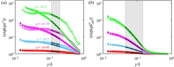
Figure 15 illustrates the wall-normal profiles of  $\langle \exp (q\tilde {u}_{AE}^{+})\rangle$ with various
 $q$ and those of
 $\langle \exp (q u^{+})\rangle$ in Case WT. There are two major differences in the scaling behaviour between the two sets of profiles. Firstly,
 $\langle \exp (q\tilde {u}_{AE}^{+})\rangle (y)$ presents a power-law decay in the mean-flow log layer (
 $3\sqrt {Re_{\tau }}< y^{+}<0.15\delta ^{+}$), which is considerably wider than the power-law region in
 $\langle \exp (q u^{+})\rangle (y)$ (
 $500< y^{+}<0.2\delta ^{+}$, consistent with Yang et al. (Reference Yang, Marusic and Meneveau2016)). Secondly,
 $\langle \exp (q\tilde {u}_{AE}^{+})\rangle (y)$ with
 $\pm q$ collapse well onto each other; therefore, the power-law factors
 $\tau _{AE}$ are the same for each pair of
 $\pm q$. No similar behaviour is observed in
 $\langle \exp (q u^{+})\rangle (y)$.
Wall-normal variation of MGF of (a)  $u$ and (b)
 $\tilde {u}_{AE}$ in Case WT for
 $q=\pm 0.45,q=\pm 0.9,q=\pm 1.35,q=\pm 1.8$. Grey patches indicate the flow region with a power-law scaling, i.e.
 $500< y^{+}<0.2\delta ^{+}$ in (a) and
 $3\sqrt {Re_{\tau }}< y^{+}<0.15\delta ^{+}$ in (b). Dash-dotted lines in black represent the linear fit of the power-law scaling in log–log plot.

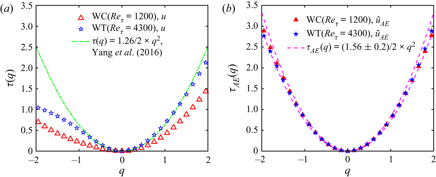
The second difference can be further quantified by figure 16, in which  $\tau (q)$ of
 $u$ and
 $\tau _{AE}(q)$ of
 $\tilde {u}_{AE}$ in the range of
 $q=[-2,2]$ are compared with the quadratic scaling of (5.4) and (5.5). Note that, for the former, the scaling constant
 $C$ takes the value of
 $A_1/2=1.26/2$ that has been suggested by Yang et al. (Reference Yang, Marusic and Meneveau2016), while for the latter,
 $C=A^{AE}_1/2=(1.56\pm 0.10)/2$, with the magnitude of
 $A^{AE}_1$ being estimated from the log-law scaling of
 $\langle \tilde {u}_{AE}^{2+}\rangle (y)$ in § 4.1. It is interesting to see that for all the tested cases, the curves of
 $\tau _{AE}(q)$ follow well the prediction of (5.4) and (5.5). As a contrast, only the positive-value part of
 $\tau (q)$ in Case WT (with higher
 $Re_\tau$) presents a similar scaling behaviour.
Power-law exponents  $\tau (q)$ of MGF of (a)
 $u$ and (b)
 $\tilde {u}_{AE}$.

Finally, it has been checked that neither superstructure-like POD eddies nor wall-detached POD eddies present a Gaussian behaviour of the MGF similar to that shown in figure 16(b). The corresponding results are not shown here for brevity.
5.3. Scaling of structure functions
Kolmogorov (Reference Kolmogorov1941) assumed that turbulent motions at high  $Re$ are self-similar in the inertial subrange of the energy cascade. This assumption leads to a power-law scaling of the
 $n$th-order longitudinal SFs of fluctuating velocities being gapped at a separation of
 $r_x$, i.e.
 \begin{equation} \langle{\rm \Delta} u^{|n|}\rangle(r_x)=\langle |u(\boldsymbol{x}+r_x)-u(\boldsymbol{x})|^{n}\rangle \propto r_x^{\zeta_n}. \end{equation}
According to Carter & Coletti (Reference Carter and Coletti2017),  ${\rm \Delta} u^{|n|}$ is calculated from the absolute value of the velocity difference to improve statistical convergence of the odd-order moments. By assuming that all statistically averaged quantities at length scale
 $r_x$ depend only on the mean dissipation rate, the so-called K41 scaling of the power-law exponents, i.e.
 \begin{equation} \zeta_n=\frac{n}{3},\end{equation}
was expected. Nevertheless, the intermittency of the energy cascade was found to deviate  $\zeta _n$ from the K41 scaling (Sreenivasan & Antonia Reference Sreenivasan and Antonia1997; Siebert, Shaw & Warhaft Reference Siebert, Shaw and Warhaft2009). She & Leveque (Reference She and Leveque1994) assumed a hierarchical distribution of the energy dissipation rate in the inertial subrange and proposed a so-called SL model for
 $\zeta _n$, i.e.
 \begin{equation} \zeta_n=\frac{n}{9}+2\left[1-\left(\frac{2}{3}\right)^{n/3}\right].\end{equation}
The validity of the SL model was proved in a TBL at  $Re_\tau =2800{\sim} O(10^{6})$ by de Silva et al. (Reference de Silva, Marusic, Woodcock and Meneveau2015), who estimated
 $\zeta _n$ directly from the power-law scaling of (5.6) in the Kolmogorov inertial subrange.
For low-to-moderate  $Re$, the inertial subrange is rather limited. This inhibits an accurate estimation of
 $\zeta _n$. Such a limitation can be avoided by extended self-similarity (ESS) (Benzi et al. Reference Benzi, Ciliberto, Tripiccione, Baudet, Massaioli and Succi1993). ESS describes a power-law correlation between any two arbitrary-order SFs in a wide scale range (extending from the inertial subrange down to the near-dissipative scale). Choosing the third-order SF as the baseline, (5.6) can be reformulated as
 \begin{equation} \langle{\rm \Delta} u^{|n|}\rangle \propto \langle{\rm \Delta} u^{|3|}\rangle^{\zeta_n}.\end{equation}
ESS provides a way of accurately estimating  $\zeta _n$. In this subsection, the scaling behaviour of high-order longitudinal SFs of either
 $u$ or its reduced-order components is examined with the help of ESS analysis. SFs contributed by various POD eddies are denoted as
 $\langle {\rm \Delta} \tilde {u}_{\chi }^{|n|}\rangle$, and the corresponding power-law exponents are
 $\zeta ^{\chi }_n$, with
 $\chi$ being
 ${SU}$,
 ${AE}$,
 ${DE}$,
 ${SS}$ or the linear combination of them.
Figure 17(a) illustrates  $\langle {\rm \Delta} u^{|n|}\rangle$ or
 $\langle {\rm \Delta} \tilde {u}_{AE}^{|n|}\rangle$ as a function of
 $r_x$ in Case WT, both of which present the power-law scaling of (5.6) in the scale range of
 $0.02< r_x/\delta <0.13$ only when
 $n\le 3$. On the other hand, as shown in figure 17(b), the ESS scaling of (5.9) is evident until
 $n=8$. It is noted that such an ESS behaviour is also seen in
 $\langle {\rm \Delta} \tilde {u}_{AE}^{|n|}\rangle$,
 $\langle {\rm \Delta} \tilde {u}_{DE}^{|n|}\rangle$ and
 $\langle {\rm \Delta} \tilde {u}_{SU}^{|n|}\rangle$.
Log–log plots of the  $n$th-order SFs as a function of (a)
 $r_x/\delta$ and (b) the third-order SFs at the wall-normal position of
 $y/\delta = 0.05$. Only results of Case WT are presented for brevity. Hollow and solid markers denote SFs of
 $u$ and
 $\tilde {u}_{AE}$, respectively. The grey patch in (a) indicates the valid inertial subrange for a power-law scaling of
 $\langle {\rm \Delta} u^{|n|}\rangle \propto r_x$, which is illustrated by a blue solid line for the
 $3^{rd}$ SFs. In (b), solid lines and dash-dotted lines in black indicate the ESS power-law fit of SFs of
 $u$ and
 $\tilde {u}_{AE}$, respectively. The fitting range is the valid inertial subrange shown in (a).

To fairly evaluate the scaling factor via (5.9), the least-square linear fitting is applied to the curves of  $\log \langle {\rm \Delta} \tilde {u}_{\chi }^{|n|}\rangle {\sim} \log \langle {\rm \Delta} \tilde {u}_{\chi }^{|3|}\rangle$ in the valid inertial subrange, which is the scale range where a linear correlation of
 $\langle {\rm \Delta} u^{|3|}\rangle \propto r_x$ holds (Benzi et al. Reference Benzi, Ciliberto, Tripiccione, Baudet, Massaioli and Succi1993). Figure 18 summarizes
 $\zeta _n$,
 $\zeta ^{SU}_n$,
 $\zeta ^{AE}_n$,
 $\zeta ^{DE}_n$ and
 $\zeta ^{AD}_n$ of Case WC and Case WT at
 $y/\delta =0.05$, 0.1, 0.2 and 0.4. It is shown that the SL model works well for
 $\zeta _n$ of full-order
 $u$, consistent with the observation of de Silva et al. (Reference de Silva, Marusic, Woodcock and Meneveau2015). On the other hand,
 $\zeta ^{SU}_n$ of superstructure-like POD eddies is slightly lower than the prediction of the K41 model, while
 $\zeta ^{AE}_n$ of wall-attached POD eddies follows it in the mean-flow log layer and below (with
 $y\le 0.15\delta$), suggesting the Gaussian behaviour of
 $\tilde {u}_{AE}$. Interestingly, the K41 model works for both
 $\zeta ^{DE}_n$ and
 $\zeta ^{AD}_n$ until
 $y/\delta =0.4$. This infers the Gaussian-like property of wall-detached motions in the higher flow layer. Finally, it has been checked that when further taking small-scale motions into account, the corresponding scaling factors return to the prediction of the SL model (the results are similar to figure 18(a) and are thus not shown for brevity).
The scaling exponent  $\zeta _n^{\chi }$ of the longitudinal SFs of (a)
 $u$, (b)
 $\tilde {u}_{SU}$, (c)
 $\tilde {u}_{AE}$, (d)
 $\tilde {u}_{DE}$ and (e)
 $\tilde {u}_{AD}$. Results of different datasets are vertically shifted for clarity. The black dash-doted lines and the red-dashed lines indicate the predictions by the SL model and the K41 model, respectively.

To our knowledge, the above observations support the existing viewpoint that the break of the K41 prediction of the longitudinal SFs of full-order  $u$ is mainly attributed to the intermittency embedded in small-scale non-Gaussian motions (Siebert et al. Reference Siebert, Shaw and Warhaft2009). Due to the limited
 $x$ span of the FOV, it is not clear whether the sub-Gaussian behaviour of superstructure-like POD eddies is a physical phenomenon or is merely caused by the insufficient ergodicity of superstructure-like motions that artificially enforces intermittency. However, it is stressed that its influence on the full-order scaling factor
 $\zeta _n$ is less critical, since owning to their larger energetic scales,
 ${\rm \Delta} u_{SU}$ (and their high-order moments) in the inertial subrange are rather smaller. On the other hand, the Gaussian behaviour of wall-detached POD eddies, which is evident in the scaling behaviour of the longitudinal SFs but not in the scaling behaviour of either the high-even-order velocity moment or MGF, is interesting. It is inferred that these passive motions might originate from Gaussian-like inertial motions in the near-wall region but gradually lose kinematic self-similarity after the detachment from the wall.
6. Concluding remarks
The main finding of the present study is that wall-attached eddies in POD modes might be regarded as the prime statistical representations of AEs in TBLs, at least in the present studied low-to-moderate  $Re$ regime (with
 $Re_{\tau }=1200{\sim} 4300$). This conclusion is based on the following three aspects of consideration.
Firstly, since AEs are usually interpreted as the statistical average of an ensemble of individual structures with similar geometric and kinematic properties, finding the statistical representation of AEs has practical meaning in turbulent modelling. Comparing with other mode decomposition methods, POD is more suitable for this purpose. The reason is that POD decomposes the spatio-temporal velocity fields into a set of POD modes that are ranked by their relative TKE contributions. The quasi-consistency between energy hierarchy and scale hierarchy, as well as the orthogonality property of POD, enables a hierarchical description of the TKE content of AEs by the combination of a subset of POD modes. Furthermore, in spite of the 2-D nature of the experiment and DNS datasets studied here, POD analysis is believed to be capable of unveiling 2-D projections of 3-D coherent motions with statistical significance.
Secondly, the spatial eigenmodes of leading-order POD modes, whose characteristic streamwise length scales are  $\lambda _x^{peak}>3\delta$, are observed to be featured by one layer of streamwise reoccurring structures that extend into the outer layer. They are believed to represent the spatial coherence of superstructure-like motions. In contrast, higher-order POD modes with
 $\lambda _x^{peak}<3\delta$ usually present a multi-layer topology, i.e. one layer of eddies that reside in the near-wall region and other layers of eddies that are physically detached from the wall. Due to the orthogonality property, discrete POD eddies in POD modes are statistically independent of each other in terms of TKE contributions. They are isolated by the clustering method and are classified into two subsets, i.e. wall-attached or wall-detached POD eddies, according to the prescribed wall-attachment condition.
Lastly, wall-attached POD eddies are deemed as statistical representations of AEs because the reduced-order  $\tilde u_{AE}$ reconstructed by them satisfy most of the kinematic properties predicted by AEH. Specifically, a hierarchical logarithmic scaling of
 $\langle \tilde {u}_{AE}^{2} \rangle \propto -A_1^{AE}\ln (y)$ is evident when enough energy (and scale) hierarchies of wall-attached POD eddies are included in the reduced-order reconstruction of
 $\tilde u_{AE}$. This resembles the feature of kinematic self-similarity of AEs. Additionally, analysis on high-even-order moments, MGF and longitudinal two-point SF indicate a quasi-Gaussian behaviour of
 $\tilde {u}_{AE}$ even in the present studied low-to-moderate
 $Re$ regime. As a contrast, none of these features are evident when the contribution of superstructure-like POD eddies are included.
The kinematic characteristics of  $\tilde u_{AE}$ is affected by the wall-attachment condition. A loose criterion of
 $y_t^{+}=60$ leads to
 $A_1^{AE}=1.56\pm 0.10$ in all three tested cases. The logarithmic scaling of high-even-order moments of
 $\tilde {u}_{AE}$, as well as the quasi-Gaussian behaviour of
 $\tilde {u}_{AE}$, suggests that the detected wall-attached POD eddies might represent an incomplete subset of AEs. Nevertheless, the scale self-similarity in
 $k_x\varPhi _{AE}$ is only evident when a strict wall-attachment condition of
 $y_t^{+}\leq 15$ is invoked. Correspondingly,
 $A_1^{AE}=1.05\pm 0.04$, consistent with
 $A_1^{AE}=0.98$ observed by Baars & Marusic (Reference Baars and Marusic2020a,Reference Baars and Marusicb) via the LCS analysis. In this sense, it is felt that the recommendation of a strict wall-attachment condition (
 $y_t^{+}\leq 15$) by previous studies (Del Alamo & Zandonade Reference Del Alamo and Zandonade2006; Lozano-Durán et al. Reference Lozano-Durán, Flores and Jiménez2012; Baars et al. Reference Baars, Hutchins and Marusic2017; Baars & Marusic Reference Baars and Marusic2020a,Reference Baars and Marusicb; Deshpande et al. Reference Deshpande, Chandran, Monty and Marusic2020) is fairly reasonable. Furthermore, the present study shows that the spectral triangle of Hu et al. (Reference Hu, Yang and Zheng2020) contains both the signatures of wall-attached and wall-detached POD eddies. In comparison, the spectral triangle of Baars et al. (Reference Baars, Hutchins and Marusic2017) well characterizes the large-scale part of
 $k_x\varPhi _{AE}$, thus is more appropriate in detecting eddies that are physically connected to the wall.
Another interesting finding is that wall-detached POD eddies also present quasi-Gaussian behaviour in the scaling of longitudinal two-point SFs of  $\tilde u_{DE}$. Referring to Marusic & Monty (Reference Marusic and Monty2019), ‘ smaller detached eddies might be remnants of eddies once attached earlier in their lifetimes’. Combining the quasi-Gaussian behaviour of
 $\tilde u_{DE}$ and the linear scaling in
 $k_x\varPhi _{AD}$, it is reasonable to treat wall-detached POD eddies as the passive fragments (or descendants) of wall-attached ones. Namely, they were directly subjected to a viscous dissipation effect under a quasi-equilibrium state in the energy cascade. For a solid justification of this inference, future attempts are required to examine the hierarchy of the energy dissipation rate of both wall-attached and wall-detached POD eddies.
Finally, it is stressed that wall-attached POD eddies only serve as statistical representations of AE-like inertial motions in a kinematic sense. Owing to the algorithm construction of POD, the POD eigenmodes only reflect the spatial pattern of statistically averaged coherent motions that have similar energy levels and scale ranges. The dynamic characteristics that describe structures’ spatio-temporal evolution cannot be accessed by the present POD analysis. This is a limitation of the present work that needs to be further considered in the future.
Acknowledgements
The authors would like to thank Professor J. Jiménez for providing the TBL DNS dataset for analysis.
Funding
This work was financially supported by the National Natural Science Foundation of China (grant Nos. 91952301, 91852206 and 11721202).
Declaration of interests
The authors report no conflict of interest.
Appendix A. Effect of the FOV and the dataset ensemble size
The effect of the size of FOV on the statistical properties of  $\tilde {u}_{AE}$ is empirically tested by truncating the dataset of Case DNS to a shorter
 $x$ span, i.e.
 ${\rm \Delta} X=4.6\delta$, which is equivalent to that of Case WT; while the effect of the number of snapshots used in POD analysis is investigated by reducing the sampling number of Case DNS from 1700 to 850. The kinematic statistics, including the cumulative
 $u$ component TKE, high-even-order moments and 1-D spectrum, are then compared with the original results.
As shown in figure 19(a), for a shorter FOV, more leading-order POD modes should be included in the low-order reconstruction of  $\tilde {u}_{AE}$ to guarantee the appearance of the log-law scaling of
 $\langle \tilde {u}_{AE}^{2}\rangle \propto \ln y$. Nevertheless, the wall-normal profiles of the cumulative
 $\varSigma ^{\infty }_i\langle \tilde {u}^{2+}_{{AE}, i}\rangle$ with two different FOV collapse with each other if the corresponding cumulative TKE proportions, i.e.
 $\varSigma _i^{\infty } e_i^{\ast }$ are comparable. Figure 19(b) reveals that the changes of high-even-order moments of
 $\tilde {u}_{AE}$ are negligible. And figure 20 shows that, apart from the scale truncation beyond
 $\lambda _x\ge 3\delta$, the pre-multiplied streamwise velocity spectra of
 $\tilde {u}_{AE}$,
 $\tilde {u}_{DE}$ or
 $\tilde {u}_{AD}$ in the scale range of
 $\lambda _x<3\delta$ are also insensitive to the FOV size. Furthermore, the primary statistical features shown in these two figures are unchanged when the size of the snapshot ensemble is reduced by half, demonstrating the convergence state of the POD analysis.
Effect of the FOV size and the number of snapshots on (a) the streamwise TKE profiles contributed by wall-attached POD eddies in all  $j$ POD modes with
 $j\ge i$ and (b) the streamwise high-even-order moments contributed by all of the wall-attached POD eddies.

Effect of the FOV size and the number of snapshots on the pre-multiplied streamwise velocity spectra of (a)  $\tilde {u}_{AE}$, (b)
 $\tilde {u}_{DE}$ and (c)
 $\tilde {u}_{AD}$. The spectra are normalized by their maximum value beyond
 $y^{+}=40$. The iso-contours are plotted at the level of 0.15 : 0.15 : 1.2.

Appendix B. Effect of wall-attachment condition
The wall-attachment condition of  $y_t^{+}=15$ is applied to the dataset of Case DNS to test its effect on the statistics of
 $\tilde {u}_{AE}$ and
 $\tilde {u}_{DE}$. As shown in figure 21(a), when the wall-attachment condition shifts from
 $y_t^{+}=60$ to
 $y_t^{+}=15$,
 $\langle \tilde {u}_{DE}^{2}\rangle$ in the mean-flow log layer and below gets enhanced, while the corresponding
 $\langle \tilde {u}_{AE}^{2}\rangle$ gets reduced. The reason is that large-scale POD eddies being weakly correlated with the wall are sorted into wall-detached subsets. As a consequence, the Townsend–Perry constant decreases to
 $A^{AE}_1=1.05\pm 0.04$. This magnitude is validated by the MGF analysis shown in figure 21(b). It is close to those reported in Baars & Marusic (Reference Baars and Marusic2020b) (
 $A^{AE}_1=0.98$) and Hu et al. (Reference Hu, Yang and Zheng2020) (
 $A^{AE}_1=1.0$). Despite of the change of
 $A^{AE}_1$, the symmetric quadratic scaling of the power-law exponents
 $\tau _{AE}(q)$ of MGF (shown in figure 21b) suggests that the quasi-Gaussian behaviour of
 $\tilde {u}_{AE}$ remains unchanged.
Effect of the wall-attachment condition on (a) the wall-normal profiles of the streamwise TKE contributed by wall-attached and wall-detached POD eddies and (b) the power-law exponent  $\tau (q)$ of MGF of
 $\tilde {u}_{AE}$ in Case DNS. Inset in (a) plots the logarithmic indicator function
 $\varXi _{AE}$ defined in (4.3), the horizontal grey patches indicate the Townsend–Perry constant of
 $A^{AE}_1=1.05\pm 0.04$ and
 $A^{AE}_1=1.56\pm 0.10$, respectively.

Furthermore, as shown in figure 22(a,b), under the condition of  $y_t^{+}=15$, both the hypotenuse in
 $k_x\varPhi _{AE}$ and the ridge line in
 $k_x\varPhi _{DE}$ follow a linear scaling of
 $\lambda _x \propto y$. Due to the orthogonal property of POD modes,
 $k_x\varPhi _{AD}$ is the sum of these two spectra. In other words, the variation of the wall-attachment condition does not change
 $k_x\varPhi _{AD}$ but affects the division boundary that separates
 $k_x\varPhi _{AD}$ into
 $k_x\varPhi _{AE}$ and
 $k_x\varPhi _{DE}$. Therefore, a linear scaling in
 $k_x\varPhi _{AD}$ (shown in figure 22c) is evident, similar to that in figure 11(c) under the condition of
 $y_t^{+}=60$.
Pre-multiplied streamwise spectra of  $\tilde {u}$ contributed by (a) wall-attached POD eddies, (b) wall-detached POD eddies and (c) both for Case DNS. Here,
 $y_t^{+}=15$. The format is the same as that in figure 11.