Introduction
As a unique one-dimension material, carbon nanotube (CNT) has exceptional mechanical and physical properties, including high tensile strength [Reference Li, Cheng, Bai, Su and Dresselhaus1, Reference Liu, Sun, Zhou, Zhu, Wang, Liu, Fan and Jiang2], strength-to-weight ratio [Reference Zhang, Li, Holesinger, Arendt, Huang, Kirven, Clapp, Depaula, Liao and Zhao3], and Young’s modulus [Reference Treacy, Ebbesen and Gibson4]. In addition, their excellent thermal, electronic, gas-storage, and fluid-conveying properties [Reference Jorio, Dresselhaus and Dresselhaus5] are attracting more and more attention and also bear potential applications in the nanoelectromechanical systems, such as nanoresonators [Reference Li and Chou6, Reference Li and Chou7], nanomotor [Reference Lohrasebi and Rafii-Tabar8], nanogear [Reference Han, Globus, Jaffe and Deardorff9], and nanoactuator [Reference Fennimore, Yuzvinsky, Han, Fuhrer, Cumings and Zettl10]. All of these applications are closely connected with the vibration behaviors of CNTs. To better design novel nanodevices, CNT’s vibration analysis is inevitable and plays an important role in the practical application.
Currently, CNT’s vibration analysis is mainly carried out by molecular dynamics (MD) simulations [Reference Durov and Ogloblya11, Reference Duan, Wang and Zhang12, Reference Wang, Hu and Guo13, Reference Ansari, Ajori and Arash14, Reference Chang15, Reference Liu and Wang16] and nonlocal continuum mechanical models [Reference Zhang, Liu and Xie17, Reference Wang and Varadan18, Reference Wang, Tan and Zhang19, Reference Lu, Lee, Lu and Zhang20, Reference Ansari and Sahmani21, Reference Yoon, Ru and Mioduchowski22, Reference Pradhan and Murmu23, Reference Mustapha and Zhong24, Reference Benzair, Tounsi, Besseghier, Heireche, Moulay and Boumia25, Reference Zhang, Liu and Xu26, Reference Murmu and Adhikari27]. Because of the difficulties associated with probing atomic-level structures via laboratory apparatuses in some cases, the former can be a good supplement to the experiments. Using MD simulations, CNT’s vibration behaviors can be simulated accurately by calculating the positions of all the carbon atoms, given the utilization of proper potentials, e.g., the interatomic potential developed by Tersoff [Reference Tersoff28], the reactive empirical bond order potential [Reference Brenner, Shenderova, Harrison, Stuart, Ni and Sinnott29], or the adaptive intermolecular reactive empirical bond order potential [Reference Stuart, Tutein and Harrison30]. However, fully MD simulations in the engineering cases would be extremely difficult and computationally expensive. Therefore, simplified mechanical models are necessary to predict the vibration behaviors of CNTs and improve the mechanical performance of nanodevices consisting of CNTs.
Different from the macroscopic materials, the mechanical properties of nanomaterials, e.g., CNTs, show remarkable size dependence. As their dimensions decrease continuously at the nanoscale, the surface-to-volume ratio increases rapidly, which influences the mechanical performance of nanomaterials to a large extent. Thus, both small-scale effect and surface effect should be considered. To describe the small-scale effect accurately, nonlocal elasticity theory [Reference Eringen31] is proposed to build the nonlocal continuum mechanical models. Based on this theory, the stress at a material point acts as the function of the strains at all points in the body. In this way, the small-scale effect is captured. Recently, researchers have implemented such a theory to investigate the vibration behaviors of CNTs. Various nonlocal beam theories are used to study the vibration responses of single-walled CNTs and multiwalled CNTs with different boundary conditions [Reference Zhang, Liu and Xie17, Reference Wang and Varadan18, Reference Wang, Tan and Zhang19, Reference Lu, Lee, Lu and Zhang20, Reference Ansari and Sahmani21]. Herein, CNTs with different lengths and diameters are discussed. In addition, the effects of elastic substrate modulus [Reference Yoon, Ru and Mioduchowski22, Reference Pradhan and Murmu23, Reference Mustapha and Zhong24], temperature change [Reference Benzair, Tounsi, Besseghier, Heireche, Moulay and Boumia25], and axial preloading [Reference Zhang, Liu and Xu26, Reference Murmu and Adhikari27], on the vibration behaviors are also investigated, based on one or more nonlocal beam models. Nevertheless, the research results from different nonlocal beam models, such as nonlocal Timoshenko and Euler–Bernoulli beam models, have not been compared in detail. Moreover, the surface effect on the vibration response is also untouched.
In this work, we analyze the size effect on the vibration response of CNTs. First, size effects, including the nonlocal small-scale effect and surface effect, are demonstrated by deriving the modified nonlocal Euler–Bernoulli and Timoshenko beam models for vibration analysis. Second, numerical experiments are carried out to obtain the vibration characteristics of CNTs with consideration of different vibration mode order and the fundamental response of the circular frequency to their dimension. Finally, the influences of several factors, i.e., elastic substrate modulus, temperature change, and axial preloading, on the circular frequency and their size-dependence are also illustrated.
Size effect
Small-scale effect and surface effect are two typical characteristics of size effect for nanomaterials. For small-scale effect, nonlocal elastic model, rather than classical continuum model, is implemented to describe accurately the mechanical performance of CNTs, and the corresponding elastic constitutive equation can be shown as [Reference Zhang, Yao and Sun32]
 $$\left\{ \matrix{ \sigma \left( x \right) - {\left( {{e_0}a} \right)^2}{{{\partial ^2}\sigma \left( x \right)} \over {\partial {x^2}}} = E\varepsilon \left( x \right) \hfill \cr \tau \left( x \right) - {\left( {{e_0}a} \right)^2}{{{\partial ^2}\tau \left( x \right)} \over {\partial {x^2}}} = G\gamma \left( x \right) \hfill \cr} \right.\quad .$$
Herein, σ(x) and τ(x) are normal and shear stresses on the cross section along the longitudinal direction of CNTs, respectively. ε(x) and γ(x) are the corresponding normal and shear strains. e 0 is a material constant which can be determined through MD simulations, and a is the internal characteristic length. Besides, E and G are the Young’s modulus and shear modulus of CNTs, respectively.
For surface effect, surface elasticity and surface stress are taken into account. The effective flexural rigidity (EI)* of CNTs is given as [Reference Zhang, Yao and Sun32]
 $${\left( {EI} \right)^ * } = EI + {\pi \over 8}S{\left( {d + t} \right)^3}\quad ,$$
where I, S, d, and t are the bending rotary inertia of the cross section, the surface modulus, CNT’s diameter, and its wall thickness, respectively. It is worth noting that we focus on the vibration behavior of single-walled CNTs embedded in the elastic substrate. For simplification, only simply supported boundary condition at the two ends is discussed.
Modified Euler–Bernoulli beam model
For Euler–Bernoulli beams, shear deformation and cross-sectional rotary inertia are neglected. Similar to the form for the classical Euler–Bernoulli beam theory, the differential governing equation for CNT’s vibration behavior with consideration of small-scale effect and surface effect can be given as
 $$\eqalign{\matrix{ {{{\left( {EI} \right)}^{\rm{*}}}{{{\partial ^4}w} \over {\partial {x^4}}} + \left[ { - \left( {N + {H^0}} \right){{{\partial ^2}w} \over {\partial {x^2}}} + {{\left( {{e_0}a} \right)}^2}\left( {N + {H^0}} \right){{{\partial ^4}w} \over {\partial {x^4}}}} \right] }\cr+ \left[ {\rho A{{{\partial ^2}w} \over {\partial {t^2}}} - {{\left( {{e_0}a} \right)}^2}\rho A{{{\partial ^4}w} \over {\partial {x^2}\partial {t^2}}}} \right] = 0\quad,} \cr} \quad$$
where A, w, ρ, and N are the cross-sectional area, the beam deflection, the mass density, and the axial load, respectively. In addition, H 0 = 2τ0(d + t), where τ0, d, and t are CNT’s residual surface stress, its diameter, and wall thickness, respectively. Thus, the internal forces can be expressed as
 $$\left\{ \matrix{ M = - {\left( {EI} \right)^*}{{{\partial ^2}w} \over {\partial {x^2}}} - {\left( {{e_0}a} \right)^2}\left[ {\left( {N + {H^0}} \right){{{\partial ^2}w} \over {\partial {x^2}}} - \rho A{{{\partial ^2}w} \over {\partial {t^2}}}} \right] \hfill \cr Q = - {\left( {EI} \right)^*}{{{\partial ^3}w} \over {\partial {x^3}}} - {\left( {{e_0}a} \right)^2}\left[ {\left( {N + {H^0}} \right){{{\partial ^3}w} \over {\partial {x^3}}} - \rho A{{{\partial ^3}w} \over {\partial x\partial {t^2}}}} \right] \hfill \cr} \right.\quad ,$$
where M is the bending moment and Q is the shear force on the cross section. Based on the separated variable method, the general solution of Eq. (3) can be given as
 $$w\left( {x,t} \right) = W\left( x \right){e^{{\rm{i}}\omega t}}\quad .$$
Substituting Eq. (5) into Eq. (3), one can obtain
 $$\eqalignb{\left\{ \!\!\!\!\!\!\matrix{ \left[ {{{\left( {EI} \right)}^*} + {{\left( {{e_0}a} \right)}^2}\left( {N + {H^0}} \right)} \right]{{{\partial ^4}W} \over {\partial {x^4}}} \cr+ \left[ {{{\left( {{e_0}a} \right)}^2}{\omega ^2}\rho A - \left( {N + {H^0}} \right)} \right]{{{\partial ^2}W} \over {\partial {x^2}}} - {\omega ^2}\rho AW = 0 \hfill \cr {G_1}{{{\partial ^4}W} \over {\partial {x^4}}} + {G_2}{{{\partial ^2}W} \over {\partial {x^2}}} + {G_3}W = 0 \hfill \cr} \right.\quad .$$
Herein, G 1 = (EI)* + (e 0a)2(N + H 0), G 2 = −(N + H 0) + (e 0a)2ω2ρA, and G 3 = −ω2ρA. The general solution of Eq. (6) is
 $$W\left( x \right) = {c_1}\sin \left( {\alpha x} \right) + {c_2}\cos \left( {\alpha x} \right) + {c_3}{e^{\beta x}} + {c_4}{e^{ - \beta x}}\quad ,$$
where α > 0, β > 0,  ${\alpha ^2} = {{\sqrt {G_2^2 - 4{G_1}{G_3}} + {G_2}} \over {2{G_1}}}$, and
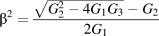 ${\beta ^2} = {{\sqrt {G_2^2 - 4{G_1}{G_3}} - {G_2}} \over {2{G_1}}}$. Then,
 $${\omega ^2} = {{\left[ {{{\left( {EI} \right)}^*} + {{\left( {{e_0}a} \right)}^2}\left( {N + {H^0}} \right)} \right]{\alpha ^2} + \left( {N + {H^0}} \right)} \over {\left[ {1 + {{\left( {{e_0}a} \right)}^2}{\alpha ^2}} \right]\rho A}}{\alpha ^2}\quad ,$$
where we can find the size effect by comparing this solution [Eq. (8)] and the classical solution 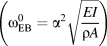 $\left( {\omega _{{\rm{EB}}}^0 = {\alpha ^2}\sqrt {{{EI} \over {\rho A}}} } \right)$. In this way, size-dependent vibration analysis of CNTs can be simplified into the determination of α with the simply supported boundary condition at the two ends. Herein, the value of α should avoid the possible situation where c 1, c 2, c 3, and c 4 in Eq. (7) have the value of zero at the same time. Combining Eqs. (4), (5), and (7), we can obtain the rotation angel of the cross section
 $${{{\rm{d}}W} \over {{\rm{d}}x}} = {c_1}\alpha \cos \left( {\alpha x} \right) - {c_2}\alpha \sin \left( {\alpha x} \right) + {c_3}\beta {e^{\beta x}} - {c_4}\beta {e^{ - \beta x}}\quad ,$$
and the internal force
 $$\left\{ \matrix{ M = - {( {{\rm{i}}\omega } )^2}{( {{e_0}a} )^2}\rho A[ {{c_1}\sin ( {\alpha x} ) + {c_2}\cos ( {\alpha x} ) + {c_3}{e^{\beta x}} }\cr{+ {c_4}{e^{ - \beta x}}} ]{e^{{\rm{i}}\omega t}} - [ {{{( {EI} )}^*} + {{( {{e_0}a} )}^2}( {N + {H^0}} )} ] \hfill [ { - {c_1}{\alpha ^2}\sin ( {\alpha x} ) }\cr{ - {c_2}{\alpha ^2}\cos ( {\alpha x} ) + {c_3}{\beta ^2}{e^{\beta x}} + {c_4}{\beta ^2}{e^{ - \beta x}}} ]{e^{{\rm{i}}\omega t}} \hfill \cr Q = {{\partial M} \over {\partial x}} \hfill \cr} \right.\quad .$$
Simply supported boundary condition at the two ends can be expressed as
 $$\left\{ \matrix{ w\left( {0,t} \right) = 0,M\left( {0,t} \right) = 0 \hfill \cr w\left( {L,t} \right) = 0,M\left( {L,t} \right) = 0 \hfill \cr} \right.\quad .$$
Substituting Eq. (11) into Eq. (10), we can obtain
 $$\left\{ \matrix{ {c_2} + {c_3} + {c_4} = 0 \hfill \cr - {c_2}{\alpha ^2} + {c_3}{\beta ^2} + {c_4}{\beta ^2} = 0 \hfill \cr {c_1}\sin \left( {\alpha L} \right) + {c_2}\cos \left( {\alpha L} \right) + {c_3}{e^{\beta L}} + {c_4}{e^{ - \beta L}} = 0 \hfill \cr - {c_1}{\alpha ^2}\sin \left( {\alpha L} \right) - {c_2}{\alpha ^2}\cos \left( {\alpha L} \right) + {c_3}{\beta ^2}{e^{\beta L}} + {c_4}{\beta ^2}{e^{ - \beta L}} = 0 \hfill \cr} \right.\quad .$$
To make sure there are nonzero solutions for c 1, c 2, c 3, and c 4, the value of the corresponding coefficient determinant should equal to zero. Thus, we can get
 $$\sin \left( {\alpha L} \right) = 0 \Rightarrow \alpha = {{n\pi } \over L}\quad .$$
Then, Eq. (13) is substituted into Eq. (8) and the circular frequency of nanobeam structure with the simply supported boundary conditions at both ends can be obtained.
As for simply supported boundary conditions at both ends, the deflection of CNTs embedded in the elastic substrate can be further set as
 $$w\left( {x,t} \right) = {W_{\max }}\sin \left( {\lambda x} \right){e^{{\rm{i}}\omega t}}\quad ,$$
where λ = nπ/L. ω and W max are the circular frequency and the deflection amplitude, respectively. Thus, the corresponding governing equation is
 $${{{\left( {EI} \right)}^*}{{{\partial ^4}w} \over {\partial {x^4}}} + \left[ { - \left( {N + {H^0} + {k_{\rm{G}}}} \right){{{\partial ^2}w} \over {\partial {x^2}}} + {{\left( {{e_0}a} \right)}^2}\left( {N + {H^0} + {k_{\rm{G}}}} \right){{{\partial ^4}w} \over {\partial {x^4}}}} \right] <$$><$$>+ \left[ {{k_{\rm{W}}}w - {{\left( {{e_0}a} \right)}^2}{k_{\rm{W}}}{{{\partial ^2}w} \over {\partial {x^2}}}} \right]} { + \left[ {\rho A{{{\partial ^2}w} \over {\partial {x^2}}} - {{\left( {{e_0}a} \right)}^2}\rho A{{{\partial ^4}w} \over {\partial {t^2}\partial {x^2}}}} \right] <$$><$$>+ \left[ { - \rho I{{{\partial ^4}w} \over {\partial {t^2}\partial {x^2}}} + {{\left( {{e_0}a} \right)}^2}\rho I{{{\partial ^6}w} \over {\partial {t^2}\partial {x^4}}}} \right] = 0} } \quad ,$$
where k W and k G are the normal Winkler modulus and the Pasternak shear modulus, respectively. Because of thermomechanical coupling effect, the corresponding axial load N consists of two parts: one part (N M) caused by the axial mechanical preloading and the other part (N T) caused by thermal expansion or contraction [Reference Zhang, Liu and Zhao33]. Hence, the axial load can be given as
 $$N = {N_{\rm{M}}} + {N_{\rm{T}}} = {N_{\rm{M}}} - {{EA} \over {1 - 2\nu }}{\alpha _x}\Delta T\quad ,$$
where αx, ΔT, and ν are the thermal expansion coefficient along the axial direction, the temperature change, and the Poisson ratio, respectively. Substituting Eq. (14) into Eq. (15), we can get
 $${{{\left( {EI} \right)}^*}{\lambda ^4} + \left( {N + {H^0} + {k_{\rm{G}}}} \right){\lambda ^2}\left[ {1 + {{\left( {{e_0}a} \right)}^2}{\lambda ^2}} \right] <$$><$$>+\,\, {k_{\rm{W}}}\left[ {1 + {{\left( {{e_0}a} \right)}^2}{\lambda ^2}} \right]} { = \rho A{\omega ^2}\left[ {1 + {{\left( {{e_0}a} \right)}^2}{\lambda ^2}} \right] <$$><$$>\!\!\!\!\!\!\!\!\!\!\!\!\!+\,\, \rho I{\lambda ^2}{\omega ^2}\left[ {1 + {{\left( {{e_0}a} \right)}^2}{\lambda ^2}} \right]} } \quad ,$$
and the circular frequency can be given as
 $$\omega = \sqrt {{{{{\left( {EI} \right)}^*}{\lambda ^4} + \left( {N + {H^0} + {k_{\rm{G}}}} \right){\lambda ^2}\left[ {1 + {{\left( {{e_0}a} \right)}^2}{\lambda ^2}} \right] + {k_{\rm{W}}}\left[ {1 + {{\left( {{e_0}a} \right)}^2}{\lambda ^2}} \right]} \over {\left( {\rho A + \rho I{\lambda ^2}} \right)\left[ {1 + {{\left( {{e_0}a} \right)}^2}{\lambda ^2}} \right]}}\quad } .$$
For Euler–Bernoulli beams, the influence of cross-sectional rotary inertia is often ignored. Then, we can get
 $${\omega _{{\rm{EB}}}} = \sqrt {{{{{\left( {EI} \right)}^*}{\lambda ^4} + \left( {N + {H^0} + {k_{\rm{G}}}} \right){\lambda ^2}\left[ {1 + {{\left( {{e_0}a} \right)}^2}{\lambda ^2}} \right] + {k_{\rm{W}}}\left[ {1 + {{\left( {{e_0}a} \right)}^2}{\lambda ^2}} \right]} \over {\rho A\left[ {1 + {{\left( {{e_0}a} \right)}^2}{\lambda ^2}} \right]}}} \quad .$$
Furthermore, by neglecting surface effect and the influence of elastic substrate, axial preloading and temperature change, the circular frequency is reduced to
 $${\omega _{{\rm{EB}} - {\rm{NL}}}} = {\lambda ^2}\sqrt {{{EI} \over {\rho A\left[ {1 + {{\left( {{e_0}a} \right)}^2}{\lambda ^2}} \right]}}} = {{\omega _{{\rm{EB}}}^0} \over {\sqrt {1 + {{\left( {{e_0}a} \right)}^2}{\lambda ^2}} }}\quad ,$$
which is consistent with the solution from the nonlocal elasticity framework. Herein,  $\omega _{{\rm{EB}}}^0 = {\lambda ^2}\sqrt {{{EI} \over {\rho A}}}$ is the circular frequency for the classic Euler–Bernoulli beam model.
Modified Timoshenko beam model
For Timoshenko beam, shear deformation and rotary inertia are considered. Similar to the deduction of the modified Euler–Bernoulli beam model, the basic governing equation for the modified Timoshenko beam model is written as
 $$\left\{ \matrix{ {( {EI} )^*}{{{\partial ^2}\psi } \over {\partial {x^2}}} - \kappa GA( {{{\partial w} \over {\partial x}} + \psi } ) = \rho I{{{\partial ^2}\psi } \over {\partial {t^2}}} - {( {{e_0}a} )^2}\rho I{{{\partial ^4}\psi } \over {\partial {t^2}\partial {x^2}}} \hfill \cr \kappa GA{\partial \over {\partial x}}( {{{\partial w} \over {\partial x}} + \psi } ) + [ {\left( {N + {H^0}} ){{{\partial ^2}w} \over {\partial {x^2}}} - {{( {{e_0}a} )}^2}( {N + {H^0}} ){{{\partial ^4}w} \over {\partial {x^4}}}} \right] }\cr{ + \hfill \cr \left[ { - {k_{\rm{W}}}w + {{( {{e_0}a} )}^2}{k_{\rm{W}}}{{{\partial ^2}w} \over {\partial {x^2}}}} \right] + \left[ {{k_{\rm{G}}}{{{\partial ^2}w} \over {\partial {x^2}}} - {{( {{e_0}a} )}^2}{k_{\rm{G}}}{{{\partial ^4}w} \over {\partial {x^4}}}} \right] }\cr{ = \rho A{{{\partial ^2}w} \over {\partial {t^2}}} - {( {{e_0}a} )^2}\rho A{{{\partial ^4}w} \over {\partial {t^2}\partial {x^2}}} \hfill \cr} \right\quad .$$
As mentioned above, the axial load N is divided into N M and N T. Considering the simple boundary conditions at both ends of CNTs, we can take the deflection expression as
 $$w\left( {x,t} \right) = {W_{\max }}\sin \left( {\lambda x} \right){e^{{\rm{i}}\omega t}}\quad ,$$
and
 $$\psi \left( {x,t} \right) = {\Psi _{\max }}\cos \left( {\lambda x} \right){e^{{\rm{i}}\omega t}}\quad .$$
Herein, λ = nπ/L and ω is the circular frequency. W max and Ψmax are the amplitudes of the deflection and the moment slope, respectively. Substituting Eqs. (22) and (23) into Eq. (21), we can obtain
 $$\left\{ \matrix{ \kappa GA\lambda {W_{\max }} +\left[ {{{( {EI} )}^*}{\lambda ^2} + \kappa GA - \rho I{\omega ^2} - {{( {{e_0}a} )}^2}\rho I{\lambda ^2}{\omega ^2}} \right] \cr {\Psi _{\max }} = 0 \hfill \cr \left[ \matrix{ \kappa GA{\lambda ^2} + \!( {N + {H^0} + {k_{\rm{G}}}} ){\lambda ^2} + {( {{e_0}a} )^2}( {N \!+ {H^0} \!+ \!{k_{\rm{G}}}} ){\lambda ^4} \hfill \cr + {k_{\rm{W}}} + {( {{e_0}a} )^2}{k_{\rm{W}}}{\lambda ^2} - \rho A{\omega ^2} - {( {{e_0}a} )^2}\rho A{\lambda ^2}{\omega ^2} \hfill \cr} \right] \cr {W_{\max }} + \kappa GA\lambda {\Psi _{\max }} = 0 \hfill \cr} \right.\quad .$$
To make sure that Eq. (24) has nonzero solutions for W max and ψmax, the coefficient determinant should be zero. In this way, Eq. (24) can be simplified into
 $${{{\left( {{\omega ^2}} \right)}^2} - {{\left( {N + {H^0} + {k_{\rm{G}}}} \right){\lambda ^2}} \over {\rho A}}{\omega ^2} - {{{{\left( {EI} \right)}^*}{\lambda ^2} + \kappa GI{\lambda ^2} + \kappa GA} \over {\rho I\left[ {1 + {{\left( {{e_0}a} \right)}^2}{\lambda ^2}} \right]}}{\omega ^2} <$$><$$>- {{{k_{\rm{W}}}} \over {\rho A}}{\omega ^2}} { + \left( {N + {H^0} + {k_{\rm{G}}}} \right){\lambda ^2}{{{{\left( {EI} \right)}^*}{\lambda ^2} + \kappa GA} \over {{\rho ^2}AI\left[ {1 + {{\left( {{e_0}a} \right)}^2}{\lambda ^2}} \right]}} <$$><$$>+ {{{{\left( {EI} \right)}^*}\kappa G{\lambda ^4}} \over {{\rho ^2}I{{\left[ {1 + {{\left( {{e_0}a} \right)}^2}{\lambda ^2}} \right]}^2}}} + } {{k_{\rm{W}}}{{{{\left( {EI} \right)}^*}{\lambda ^2} + \kappa GA} \over {{\rho ^2}AI\left[ {1 + {{\left( {{e_0}a} \right)}^2}{\lambda ^2}} \right]}} \!= 0} } \quad .$$
By solving Eq. (25), we can obtain two circular frequencies (ωT1 and ωT2). For the lower circular frequency, the corresponding vibration is flexural vibration; for the higher circular frequency, the corresponding vibration is shear vibration. When the effect of the elastic substrate is neglected, Eq. (25) is converted into
 $$\matrix{ {{{\left( {{\omega ^2}} \right)}^2} - {{\left( {N + {H^0}} \right){\lambda ^2}} \over {\rho A}}{\omega ^2} - {{{{\left( {EI} \right)}^*}{\lambda ^2} + \kappa GI{\lambda ^2} + \kappa GA} \over {\rho I\left[ {1 + {{\left( {{e_0}a} \right)}^2}{\lambda ^2}} \right]}}{\omega ^2}} \hfill \cr { + \left( {N + {H^0}} \right){\lambda ^2}{{{{\left( {EI} \right)}^*}{\lambda ^2} + \kappa GA} \over {{\rho ^2}AI\left[ {1 + {{\left( {{e_0}a} \right)}^2}{\lambda ^2}} \right]}} + {{{{\left( {EI} \right)}^*}\kappa G{\lambda ^4}} \over {{\rho ^2}I{{\left[ {1 + {{\left( {{e_0}a} \right)}^2}{\lambda ^2}} \right]}^2}}} = 0} \hfill \cr} \quad .$$
When the axial load and the surface effect are further ignored, we can obtain the following equation to solve the circular frequency of Timoshenko beam in the nonlocal elasticity framework:
 $${{E\kappa G} \over {{\rho ^2}}}{\lambda ^4} - \left[ {1 + {{\left( {{e_0}a} \right)}^2}{\lambda ^2}} \right]\left\{ {\left[ {{{\kappa GA} \over {\rho I}} + \left( {{E \over \rho } + {{\kappa G} \over \rho }} \right){\lambda ^2}} \right] <$$><$$>- \left[ {1 + {{\left( {{e_0}a} \right)}^2}{\lambda ^2}} \right]{\omega ^2}} \right\}{\omega ^2} = 0\quad .$$
When  ${c_1} = \sqrt {{E / \rho }}$,
 ${c_2} = \sqrt {{{\kappa G} / \rho }}$, and
 ${r_0} = \sqrt {{I / A}}$ are taken, Eq. (27) can be converted into
 $$c_1^2r_0^2{\lambda ^4} - \left[ {1 + {{\left( {{e_0}a} \right)}^2}{\lambda ^2}} \right]\left\{ {1 + r_0^2\left( {1 + {{c_1^2} \over {c_2^2}}} \right){\lambda ^2} <$$><$$>- \left[ {1 + {{\left( {{e_0}a} \right)}^2}{\lambda ^2}} \right]{{r_0^2} \over {c_2^2}}{\omega ^2}} \right\}{\omega ^2} = 0\quad .$$
The solution of Eq. (28) is
 $${\omega _{{\rm{T}} - {\rm{NL}}}} = {{\omega _{\rm{T}}^0} \over {\sqrt {1 + {{\left( {{e_0}a} \right)}^2}{\lambda ^2}} }}\quad ,$$
where  $\omega _{\rm{T}}^0$ denotes the circular frequency for the classical Timoshenko beam model and can be shown as
 $$\omega _{\rm{T}}^0 = \sqrt {{1 \over 2}\left[ {\left( {c_1^2 + c_2^2} \right){\lambda ^2} + {{c_2^2} \over {r_0^2}}} \right] \pm \sqrt {{1 \over 4}{{\left[ {\left( {c_1^2 + c_2^2} \right){\lambda ^2} + {{c_2^2} \over {r_0^2}}} \right]}^2} - c_1^2c_2^2{\lambda ^4}} } \quad .$$
Arash et al. [Reference Arash and Wang34] pointed out that the influence of the nonlocal small-scale effect on the circular frequency is negligible for the shear force term of Timoshenko beam model. Hence, it can be removed in the following deduction. Based on this point, Eq. (21) can be converted into a more simplified form:
 $$\left\{ \matrix{ {\left( {EI} \right)^*}{{{\partial ^2}\psi } \over {\partial {x^2}}} - \kappa GA\left( {{{\partial w} \over {\partial x}} + \psi } \right) = \rho I\left[ {{{{\partial ^2}\psi } \over {\partial {t^2}}} - {{\left( {{e_0}a} \right)}^2}{{{\partial ^4}\psi } \over {\partial {t^2}\partial {x^2}}}} \right] \hfill \cr \kappa GA{\partial \over {\partial x}}\left( {{{\partial w} \over {\partial x}} + \psi } \right) + \left( {N + {H^0}} \right){{{\partial ^2}w} \over {\partial {x^2}}} = \rho A{{{\partial ^2}w} \over {\partial {t^2}}} \hfill \cr} \right.\quad .$$
Additionally, the expressions of internal forces (the bending moment and the shear force) can be reduced to
 $$\left\{ \matrix{ M = {\left( {EI} \right)^*}{{\partial \psi } \over {\partial x}} - {\left( {{e_0}a} \right)^2}\left[ {\left( {N + {H^0}} \right){{{\partial ^2}w} \over {\partial {x^2}}} - \rho A{{{\partial ^2}w} \over {\partial {t^2}}} - \rho I{{{\partial ^3}\psi } \over {\partial {t^2}\partial x}}} \right] \hfill \cr Q = \kappa GA\left( {{{\partial w} \over {\partial x}} + \psi } \right) \hfill \cr} \right.\quad .$$
The general solution of Eq. (31) can be
 $$\left\{ \matrix{ w\left( {x,t} \right) = W\left( x \right){e^{{\rm{i}}\omega t}} \hfill \cr \psi \left( {x,t} \right) = \Psi \left( x \right){e^{{\rm{i}}\omega t}} \hfill \cr} \right.\quad .$$
Substituting Eq. (33) into Eq. (31), we can obtain
 $$\left\{ \matrix{ {\left( {EI} \right)^*}{{{\partial ^2}\Psi } \over {\partial {x^2}}} - \kappa GA\left( {{{\partial W} \over {\partial x}} + \Psi } \right) + {\omega ^2}\rho I\left[ {\Psi - {{\left( {{e_0}a} \right)}^2}{{{\partial ^2}\Psi } \over {\partial {x^2}}}} \right] = 0 \hfill \cr \kappa GA\left( {{{{\partial ^2}W} \over {\partial {x^2}}} + {{\partial \Psi } \over {\partial x}}} \right) + \left( {N + {H^0}} \right){{{\partial ^2}W} \over {\partial {x^2}}} + {\omega ^2}\rho AW = 0 \hfill \cr} \right.\quad .$$
By separating variable, we further get
 $$\left\{ \matrix{ {s_1}{{{{\rm{d}}^4}W} \over {{\rm{d}}{x^4}}} + {s_2}{{{{\rm{d}}^2}W} \over {{\rm{d}}{x^2}}} + {s_3}W = 0 \hfill \cr {s_1}{{{{\rm{d}}^4}\Psi } \over {{\rm{d}}{x^4}}} + {s_2}{{{{\rm{d}}^2}\Psi } \over {{\rm{d}}{x^2}}} + {s_3}\Psi = 0 \hfill \cr} \right.\quad ,$$
where  ${s_1} = \left[ {{{\left( {EI} \right)}^*} - {{\left( {{e_0}a} \right)}^2}{\omega ^2}\rho I} \right]{{\kappa GA + \left( {N + {H^0}} \right)} \over {\kappa GA}}$,
 ${s_2} = \left[ {{{\left( {EI} \right)}^*} - {{\left( {{e_0}a} \right)}^2}{\omega ^2}\rho I} \right]{{{\omega ^2}\rho A} \over {\kappa GA}} \,\,+\,\, {\omega ^2}\rho I{{\kappa GA + \left( {N + {H^0}} \right)} \over {\kappa GA}} \,-\, \left( {N + {H^0}} \right)$, and
 ${s_3} = {{{\omega ^2}\rho A} \over {\kappa GA}}\left( {{\omega ^2}\rho I - \kappa GA} \right)$. The general solution of Eq. (35) can be expressed as
 $$\left\{ \matrix{ W\left( x \right) = {c_1}\sin \left( {\alpha x} \right) + {c_2}\cos \left( {\alpha x} \right) + {c_3}{e^{\beta x}} + {c_4}{e^{ - \beta x}} \hfill \cr \Psi \left( x \right) = {f_1}\sin \left( {\alpha x} \right) + {f_2}\cos \left( {\alpha x} \right) + {f_3}{e^{\beta x}} + {f_4}{e^{ - \beta x}} \hfill \cr} \right.\quad .$$
Herein, α > 0, β > 0,  ${\alpha ^2} = {{\sqrt {s_2^2 - 4{s_1}{s_3}} + {s_2}} \over {2{s_1}}}$, and
 ${\beta ^2} = {{\sqrt {s_2^2 - 4{s_1}{s_3}} - {s_2}} \over {2{s_1}}} = {{\sqrt {s_2^2 - 4{s_1}{s_3}} } \over {{s_1}}} - {\alpha ^2}$. Substituting Eq. (36) into Eq. (31), the coefficient relationships can be shown as
 $$\left\{ \matrix{ {f_1} = {\Omega _\alpha }{c_2},\;{f_2} = - {\Omega _\alpha }{c_1},\;{\Omega _\alpha } = \left[ {\alpha + \alpha {{\left( {N + {H^0}} \right)} \over {\kappa GA}} - {{{\omega ^2}\rho A} \over {\alpha \kappa GA}}} \right] \hfill \cr {f_3} = - {\Omega _\beta }{c_3},\;{f_4} = {\Omega _\beta }{c_4},\;{\Omega _\beta } = \left[ {\beta + \beta {{\left( {N + {H^0}} \right)} \over {\kappa GA}} + {{{\omega ^2}\rho A} \over {\beta \kappa GA}}} \right] \hfill \cr} \right.\quad .$$
Based on the modified Timoshenko beam model, the vibration analysis of single-walled CNTs is converted to the determination of the unknown coefficients in Eq. (36) with simply supported boundary condition at the two ends. To obtain the circular frequency, we only need to solve the governing equation with the condition that the coefficient determinants equal to zero. For simplification, Eq. (32) can be converted into
 $$\left\{ \matrix{ M = \left[ {{{\left( {EI} \right)}^*} - {{\left( {{e_0}a} \right)}^2}\rho I{\omega ^2}} \right]\left[ {{f_1}\alpha \cos \left( {\alpha x} \right) - {f_2}\alpha \sin \left( {\alpha x} \right) + {f_3}\beta {e^{\beta x}} - {f_4}\beta {e^{ - \beta x}}} \right]{e^{{\rm{i}}\omega t}} \hfill \cr - {\left( {{e_0}a} \right)^2}\left( {N + {H^0}} \right)\left[ { - {c_1}{\alpha ^2}\sin \left( {\alpha x} \right) - {c_2}{\alpha ^2}\cos \left( {\alpha x} \right) + {c_3}{\beta ^2}{e^{\beta x}} + {c_4}{\beta ^2}{e^{ - \beta x}}} \right]{e^{{\rm{i}}\omega t}} \hfill \cr - {\left( {{e_0}a} \right)^2}\rho A{\omega ^2}\left[ {{c_1}\sin \left( {\alpha x} \right) + {c_2}\cos \left( {\alpha x} \right) + {c_3}{e^{\beta x}} + {c_4}{e^{ - \beta x}}} \right]{e^{{\rm{i}}\omega t}} \hfill \cr Q = \kappa GA\left[ {\matrix{ {{c_1}\alpha \cos \left( {\alpha x} \right) - {c_2}\alpha \sin \left( {\alpha x} \right) + {c_3}\beta {e^{\beta x}} - {c_4}\beta {e^{ - \beta x}}} \cr { + {f_1}\sin \left( {\alpha x} \right) + {f_2}\cos \left( {\alpha x} \right) + {f_3}{e^{\beta x}} + {f_4}{e^{ - \beta x}}} \cr} } \right]{e^{{\rm{i}}\omega t}} \hfill \cr} \quad.$$
For the simply supported boundary conditions at both ends, by combining Eqs. (11) and (38), we can obtain
 $$\left\{ \matrix{ {c_2} + {c_3} + {c_4} = 0 \hfill \cr \left[ {{{\left( {EI} \right)}^*} - {{\left( {{e_0}a} \right)}^2}\rho I{\omega ^2}} \right]\left( {{f_1}\alpha + {f_3}\beta - {f_4}\beta } \right) \hfill \cr - {\left( {{e_0}a} \right)^2}\left( {N + {H^0}} \right)\left( { - {c_2}{\alpha ^2} + {c_3}{\beta ^2} + {c_4}{\beta ^2}} \right) - {\left( {{e_0}a} \right)^2}\rho A{\omega ^2}\left( {{c_2} + {c_3} + {c_4}} \right) = 0 \hfill \cr {c_1}\sin \left( {\alpha L} \right) + {c_2}\cos \left( {\alpha L} \right) + {c_3}{e^{\beta L}} + {c_4}{e^{ - \beta L}} = 0 \hfill \cr \left[ {{{\left( {EI} \right)}^*} - {{\left( {{e_0}a} \right)}^2}\rho I{\omega ^2}} \right]\left[ {{f_1}\alpha \cos \left( {\alpha L} \right) - {f_2}\alpha \sin \left( {\alpha L} \right) + {f_3}\beta {e^{\beta L}} - {f_4}\beta {e^{ - \beta L}}} \right] \hfill \cr - {\left( {{e_0}a} \right)^2}\left( {N + {H^0}} \right)\left[ { - {c_1}{\alpha ^2}\sin \left( {\alpha L} \right) - {c_2}{\alpha ^2}\cos \left( {\alpha L} \right) + {c_3}{\beta ^2}{e^{\beta L}} + {c_4}{\beta ^2}{e^{ - \beta L}}} \right] \hfill \cr - {\left( {{e_0}a} \right)^2}\rho A{\omega ^2}\left[ {{c_1}\sin \left( {\alpha L} \right) + {c_2}\cos \left( {\alpha L} \right) + {c_3}{e^{\beta L}} + {c_4}{e^{ - \beta L}}} \right] = 0 \hfill \cr} \right.\quad .$$
To make sure there are nonzero solutions for c i (i = 1–4) and f j (j = 1–4), the corresponding coefficient determinant should equal to zero. Thus, we can get
 $$\sin \left( {\alpha L} \right) = 0 \Rightarrow \alpha = {{n\pi } \over L}\quad .$$
According to the correlation between α and ω, the circular frequency for the simply supported boundary conditions at both ends is obtained. In this way, the governing equations of the circular frequency can be solved, without considering the influence of nonlocal small-scale effect on the shearing term of Timoshenko beam model.
Numerical results and discussion
For the vibration analysis of single-walled CNT embedded in the elastic substrate, the circular frequency for the modified Euler–Bernoulli beam model is illustrated as Eq. (19), whereas that for the modified Timoshenko beam model originates from the positive root of Eq. (25). Herein, the larger positive root corresponds to the circular frequency of the shear vibration, whereas the smaller one is related to the flexural vibration (the research focus in our work). When small-scale effect and surface effect are neglected, the above frequency solutions can be degraded to the circular frequencies for the classical Euler–Bernoulli and Timoshenko beam models, respectively. When the effects of elastic substrate, temperature change, and axial preloading are further removed, we can obtain the circular frequencies of the corresponding Euler–Bernoulli beam and Timoshenko beam under the classical theoretical framework (i.e.,  $\omega _{{\rm{EB}}}^0$ and
 $\omega _{\rm{T}}^0$).
For single-walled CNTs, the representative parameters used in the numerical experiments are selected as follows [Reference Sun, Yao, Liang and Han35, Reference Yao and Sun36]: bulk Young’s modulus E = 5.5 TPa, wall thickness t = 0.066 nm, nonlocal material parameter e 0 = 0.39, internal characteristic length a = 0.142 nm, residual surface stress τ0 = 25 nN/nm, surface modulus S = 50 nN/nm, thermal expansion coefficient αx = −1.6 × 10⁻⁶ K−1 at room or low temperature, and αx = 1.1 × 10⁻⁶ K−1 at high temperature.
Generally, the chiral vector of single-walled CNT is taken as (9,9) and the corresponding diameter (d) is 1.22 nm. In addition, the length–diameter ratio (L/d) is set as 12. Figure S1 in the Supplementary material shows the dependence of circular frequency on the vibration mode order n for different beam models. For both the classical and the modified beam models, the circular frequencies of single-walled CNTs increase with the increase of the vibration mode order. In addition, the computational results for the modified beam models are larger than the corresponding results for the classical beam models. Thus, small-scale effect and surface effect have non-negligible influences on the circular frequency. For the flexural vibration with a low vibration mode order, the circular frequency of Euler–Bernoulli beam is slightly higher than that of Timoshenko beam. As the vibration mode order (n) increases continuously, the circular frequency of Euler–Bernoulli beam model rises rapidly and the difference between these two models are also expanded. Compared with Timoshenko beam model, Euler–Bernoulli beam model is more sensitive to the vibration mode order. To further investigate the influence of the vibration mode order on size effect, we trace the evolution of circular frequency ratios in Fig. S2. Herein, the ratios of circular frequency reflect the size effect to some extent and are defined as
 $$\left\{ \matrix{ {r_{{\rm{EB}}}} = {{{\omega _{{\rm{EB}}}}} \over {\omega _{{\rm{EB}}}^0}} \hfill \cr {r_{\rm{T}}} = {{{\omega _{\rm{T}}}} \over {\omega _{\rm{T}}^0}} \hfill \cr} \right.\quad ,$$
where r EB and r T denote the ratios of frequency for Euler–Bernoulli beam and Timoshenko beam, respectively. ωEB,  $\omega _{{\rm{EB}}}^0$, ωT, and
 $\omega _{\rm{T}}^0$ represent the circular frequencies for the modified Euler–Bernoulli beam models, the classical Euler–Bernoulli beam model, the modified Timoshenko beam model, and the classical Timoshenko beam model, respectively. For flexural vibration, size effect is more significant when the vibration mode order is low; for shear vibration, size effect evolves nonlinearly with the increase of the vibration mode order, and there is the most optimized vibration mode order, which corresponds to the most significant size effect.
In addition, we take n = 2 to investigate the effects of nonlocal small-scale effect parameter e 0, surface modulus S, and residual surface stress τ0 on the circular frequency of single-walled CNTs. The results are shown in the Supplementary material (Figs. S3–S5). For flexural vibration, the computational results for the modified Euler–Bernoulli beam model are much larger than those for the modified Timoshenko beam, which is consistent with the case for the classical beam models. According to Fig. S3, with the increase of e 0, the circular frequencies of single-walled CNTs decrease for both flexural vibration and shear vibration. On the contrary, such a trend reverses for the cases of surface modulus S (Fig. S4) and residual surface stress τ0 (Fig. S5). Among these three factors, the effect of τ0 is most significant. Compared with surface effect (represented by S and τ0), the small-scale effect (shown in the case of e 0) plays an opposite role in the evolution of circular frequency; namely, small-scale effect makes single-walled CNT “softer” and thus easier to vibrate, whereas surface effect makes it “harder” and more difficult to vibrate. Thus, the flexural vibration of CNTs are influenced by these two effects at the same time. For shear vibration, similar conclusions are obtained, whereas the effect of e 0 is the “strongest,” compared with that of S and τ0.
Effect of structural dimensions
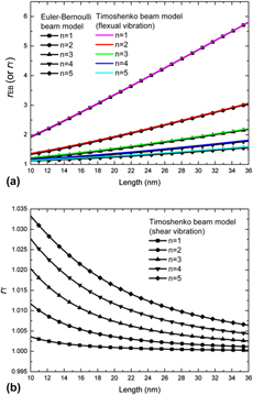
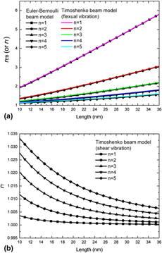
Figures 1–3 illustrate the effects of structural dimensions on the ratio of circular frequency (i.e., size effect) for the modified Euler–Bernoulli and Timoshenko beam models. With CNT’s diameter unchanged, the length–diameter ratio increases when CNT’s length increases and vice versa. As shown in Fig. 1(a) (flexural vibration), the circular frequency ratio increases with the length increasing, indicating an increasingly significant size effect. On the contrary, the reversed trend is demonstrated in Fig. 1(b) (shear vibration). For the flexural vibration, the rising rate of the circular frequency ratio is faster when the vibration mode order is lower; for the shear vibration, the higher the vibration mode order is, the faster the circular frequency ratio increases. Therefore, when CNT’s diameter is constant, its length has a remarkable influence on the size dependence of CNT’s vibration analysis.
The circular frequency ratio as a function of CNT’s length (constant diameter) for (a) flexural vibration and (b) shear vibration.

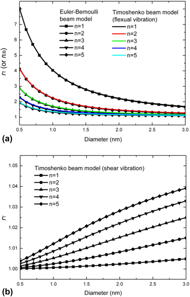
The circular frequency ratio as a function of CNT’s diameter (constant length) for (a) flexural vibration and (b) shear vibration.

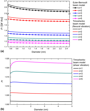
The circular frequency ratio as a function of CNT’s diameter (constant length–diameter ratio) for (a) flexural vibration and (b) shear vibration.

Similarly, with CNT’s length constant (Fig. 2), the circular frequency ratios evolve in the opposite trends for flexural vibration and shear vibration. For flexural vibration [Fig. 2(a)], as CNT’s diameter increases, the length–diameter ratio decreases, whereas size effect weakens significantly. For shear vibration [Fig. 2(b)], size effect is strengthened with the increase of CNT’s diameter. Therefore, the relationships between the performance of size effect and the length–diameter ratio are similar in both Figs. 1 and 2.
To further investigate the relationship between the circular frequency ratio and the length–diameter ratio, we keep the length–diameter ratio constant and change CNT’s diameter and its length at the same time. The results are demonstrated in Fig. 3. For flexural vibration [Fig. 3(a)], size effect becomes more prominent with the decrease of CNT’s diameter. Such a phenomenon is further strengthened when the vibration mode order is low. For shear vibration [Fig. 3(b)], when the vibration mode order is lower (e.g., n = 1–2), there is a similar trend for the relationship between CNT’s circular frequency ratio and its diameter. However, when the vibration mode order is higher (e.g., n > 2), the nonlinear correlation between the circular frequency ratio and CNT’s diameter exists. For a given vibration mode order, there is a typical diameter, which corresponds to the “strongest” size effect.
Effect of elastic substrate modulus
In many project cases, CNTs are embedded in the elastic substrates. Thus, it is necessary to investigate the impact of elastic substrate properties on the circular frequency and the ratio of frequency (i.e., the strength of size effect). Herein, we focus on the flexural vibration of CNTs, and two important parameters for elastic substrate (Winkler modulus K W and Pasternak shear modulus k G) are considered.
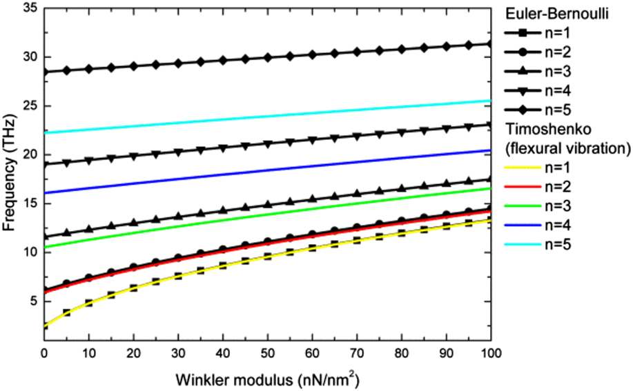
According to Figs. 4 and S6, for a given vibration mode order, the circular frequency of single-walled CNTs increases with the increase of Winkler modulus K W, suggesting that a larger Winkler modulus suppresses the vibration of single-walled CNTs and enhances their circular frequency. It should be noted that when the vibration mode order is low, the calculation results for Euler–Bernoulli beam model approximate to those of Timoshenko beam model. As the vibration mode order further increases, the frequency difference between these two models is enlarged (Fig. 4).
The circular frequency as a function of Winkler modulus for different beam models.

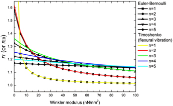
Figure 5 shows the variation of the circular frequency ratios (r EB or r T) with respect to Winkler modulus K W. Obviously, the frequency ratio, proportional to the strength of size effect, gradually decreases with the increase of Winkler modulus K W. The lower the vibration mode order is, the more rapidly the frequency ratio decreases. Specifically, for n = 1–2, as K W increases, the ratio of circular frequency drops first at a fast rate and then approaches 1 gradually at a much slower rate. For a larger n, the ratio of frequency decreases gently with the enhancement of K W. Therefore, when Winkler modulus K W is small, its slight change has a remarkable influence on the size effect of single-walled CNTs and cannot be ignored. Similar to the results in Fig. 4, the frequency difference between these two models is obvious when vibration mode order is high.
The circular frequency ratio as a function of Winkler modulus for different beam models.

Furthermore, the effects of Pasternak shear modulus k G on the vibration characteristics of CNTs are demonstrated in Figs. S7–S9. The calculation results are similar to those for Winkler modulus K W. As shown in Fig. S7–S8, the circular frequency increases with the increase of Pasternak shear modulus k G. The lower the vibration mode order is, the smaller the frequency difference between Euler–Bernoulli beam model and Timoshenko beam model is. In Fig. S9, the ratio of frequency decreases with the increase of Pasternak shear modulus k G. Similar to Winkler modulus K W, when Pasternak shear modulus k G is low, its slight change influences the frequency ratio (i.e., size effect) significantly. Additionally, as Pasternak shear modulus k G increases, the ratio of circular frequency approaches 1.
Effect of temperature change
Temperature change is the most common environmental factor for the applications of many nanodevices involving CNTs, and its influence on the mechanical behavior of CNTs has been analyzed by many researchers [Reference Zhang, Liu and Zhao33, Reference Yao and Han37]. Generally, we investigate the vibration response of CNTs at high temperature and the effects of temperature change on the circular frequency and the frequency ratio. In addition, the thermal expansion coefficient of CNTs is positive at high temperature, but negative at room or low temperature. Therefore, we can deduce an opposite conclusion for the cases at room or low temperature, according to the results at high temperature. Herein, only flexural vibration is discussed.
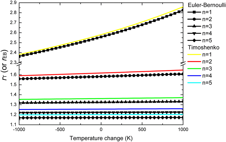
Based on the elastic substrate correlation term in the modified Euler–Bernoulli and Timoshenko beam models, we can conclude that the circular frequency of single-walled CNTs decreases with the increase of temperature changes. An example with n = 2 is shown in Fig. S10. The effect of temperature change on the frequency ratio is demonstrated in Fig. 6, where the frequency ratio rises with the temperature change increasing. For a given vibration mode order, the curves for the frequency ratio of the Timoshenko beam model always lie above those for the Euler–Bernoulli beam model. When the vibration mode order is lower, the corresponding frequency ratio varies greatly for the same temperature range. Therefore, when the value of temperature change is positive and large, it plays an important role in the performance of size effect.
The circular frequency ratio as a function of temperature change for different beam models.

Effect of axial preloading
The practical serving environment of CNTs is sophisticated. In many cases, axial preloadings can be caused by temperature change or assembly error. Therefore, it is of great importance to investigate the influence of different preloadings on the vibration behavior of CNTs. Herein, we discuss the effects of axial preloadings on the flexural circular frequency and the frequency ratio of single-walled CNTs. Based on the modified beam models we derive, the effect of axial preloading is consistent with that of Pasternak shear modulus k G. The only difference is that the value of preload can be positive (pretensile loading) or negative (precompressive loading), whereas Pasternak shear modulus can only take a positive value.
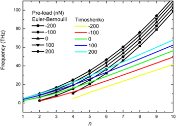
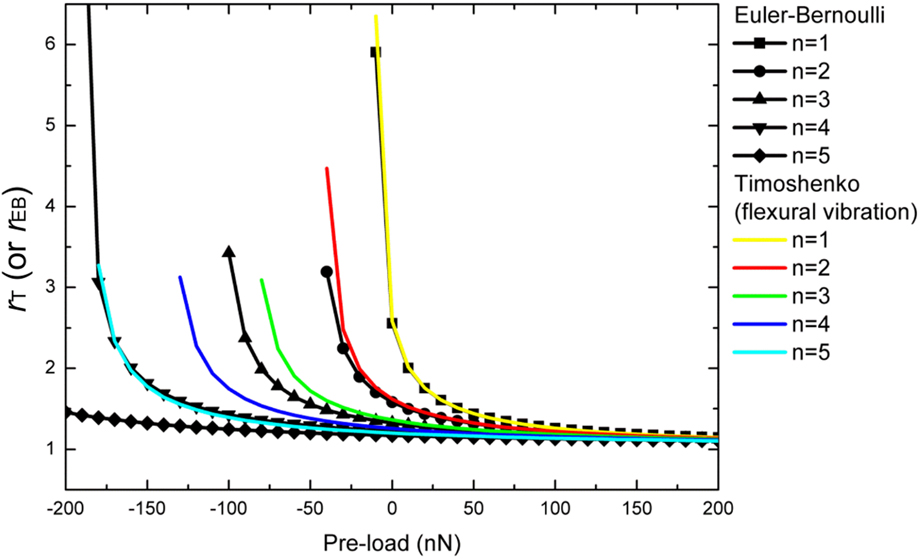
Figure 7 depicts the dependence of the circular frequency on the vibration mode order for different beam models with various preloads. According to Fig. 7, the axial pretensile loading enhances the circular frequency of single-walled CNTs, whereas the axial precompressive loading reduces the corresponding frequency. For a much larger precompressive loading, the positive root for the solution of circular frequency may not exist, because such a stress level restrains CNT’s flexural vibration severely and makes its buckling destruction easier to take place. More details are shown in Fig. S11. For a given vibration mode order, the circular frequency increases with the increase of the preload, and the frequency corresponding to modified Euler–Bernoulli beam model is higher than that for the Timoshenko beam model. The difference is enlarged, as the vibration mode order increases. Additionally, the circular ratio as a function of axial preloadings is also illustrated in Fig. 8. It is easy to find that the effect of the axial precompressive loading on the circular frequency ratio is much more significant than that of the axial pretensile loadings. As the axial precompressive loading increases, the circular frequency ratio rises sharply, and a larger precompressive loading may lead to the termination of vibration and the initiation of buckling behavior, which corresponds to no real solution for the circular frequency. On the contrary, with the increase of the axial pretensile loading, the ratio of circular frequency drops gradually, i.e., size effect gradually weakens.
The circular frequency as a function of vibration mode order for different beam models with various preloads.

The circular frequency ratio as a function of preload for different beam models.

Conclusions
By deriving the modified Euler–Bernoulli and Timoshenko beam models for CNT’s vibration behaviors and carrying out the numerical experiments, we have investigated symmetrically the influences of nonlocal small-scale effect and surface effect on the vibration response of CNTs. Our main conclusions are
(1) The size effect is directly related to the structure dimensions of CNTs. For flexural vibration, size effect, represented by the circular frequency ratio of single-walled CNT, decreases with the increase of its diameter, but increases with the increase of the length–diameter ratio; for shear vibration with n = 1–2, size effect weakens, as CNT’s diameter and length–diameter ratio increase.
(2) For flexural vibration, the circular frequency is positively correlated with Winkler modulus and Pasternak shear modulus, indicating that the elastic substrate restrains CNT’s vibration to some extent. In addition, size effect is strengthened with the decreases of Winkler modulus and Pasternak shear modulus.
(3) For flexural vibration at high temperature, the circular frequency of single-walled CNT decreases with the increase of temperature change, suggesting that temperature rise promotes the vibration response. On the other hand, the ratio of the circular frequency (i.e., the intensity of size effect) is enhanced with the increase of temperature change, suggesting that temperature rise strengthens size effect. According to the thermal expansion characteristics of CNTs, the corresponding results for room or low temperature are opposite to those for high temperature.
(4) The axial preloading has an important influence on the flexural circular frequency and the performance of size effect. The precompressive loading reduces the flexural circular frequency, but promotes the performance of size effect; the pretensile loading enhances the flexural circular frequency, but has little impact on the size dependence of CNT’s vibration response.
(5) The lower the vibration mode order is, the closer the results from the modified Euler–Bernoulli and Timoshenko beam models are. Meanwhile, the effects of different factors, including elastic substrate, temperature change, and axial preloading, are more significant at a low vibration mode order.
Supplementary material
To view supplementary material for this article, please visit https://doi.org/10.1557/jmr.2018.431.
Acknowledgments
This work was partially supported by the National Natural Science Foundation of China (Nos. 11672110, 11472110, and 11372113), the Natural Science Foundation of Guangdong Province (No. 2017A030313014), and the open projects of State Key Laboratory for Strength and Vibration of Mechanical Structures (Xi’an Jiaotong University) (No. SV2017-KF-04).