1 Introduction
Density fields in oceanic flows are often stably stratified due to spatiotemporal variations in temperature and salinity (or a combination of both). Nonlinear internal waves (NLIWs) are common features of such flow fields (particularly in the marine context), and several field studies in the ocean have shown that many NLIWs can attain near-solitary travelling wave form (for example, see Helfrich & Melville (Reference Helfrich and Melville2006) and references therein). Moreover, it is well known that such large-amplitude internal solitary waves (ISWs) show evidence of breaking through shear-induced instability. The process can be seen, for example, (i) in field observations (Moum et al. Reference Moum, Farmer, Smyth, Armi and Vagle2003; Lamb & Farmer Reference Lamb and Farmer2011; Lien, Henyey & Ma Reference Lien, Henyey and Ma2014; Zhang & Alford Reference Zhang and Alford2015), (ii) in the laboratory (Grue et al. Reference Grue, Jensen, Rusås and Sveen1999; Fructus et al. Reference Fructus, Carr, Grue, Jensen and Davies2009) and (iii) in numerical simulations (Barad & Fringer Reference Barad and Fringer2010; Carr, King & Dritschel Reference Carr, King and Dritschel2011; Almgren, Camassa & Tiron Reference Almgren, Camassa and Tiron2012). In the recent observations of Zhang & Alford (Reference Zhang and Alford2015), overturning events associated with shear instability were detected in 318 waves out of a total of 657 waves, confirming that shear-induced breaking in ISWs is a common phenomenon in oceanic flows. Reviews by Smyth & Moum (Reference Smyth and Moum2012) and Lamb (Reference Lamb2014) provide further references and a comprehensive summary of work in this area.
A commonly observed instability in stratified shear flow is the Kelvin–Helmholtz (KH) instability (Helmholtz Reference Helmholtz1868; Kelvin Reference Kelvin1871). The KH instability has been widely studied (Thorpe Reference Thorpe1973; Koop & Browand Reference Koop and Browand1979; Caulfield, Yoshida & Peltier Reference Caulfield, Yoshida and Peltier1996; Smyth, Moum & Caldwell Reference Smyth, Moum and Caldwell2001) due to the integral role it plays in the transition of a shear flow to turbulence, a classical area of investigation in theoretical fluid mechanics. Applications of KH studies include understanding mixing and transport in (i) the deep ocean (van Haren & Gostiaux Reference van Haren and Gostiaux2010), (ii) the oceanic thermocline (Thorpe Reference Thorpe2004), (iii) estuarine shear zones (Geyer et al.
Reference Geyer, Lavery, Scully and Trowbridge2010), (iv) density current overflows in the ocean (Legg Reference Legg2009) and (v) the atmosphere (Luce et al.
Reference Luce, Mega, Yamamoto, Yamamoto, Hashiguchi, Fukao, Nishi, Tajiri and Nakazato2010; Fukao et al.
Reference Fukao, Luce, Megac and Yamamoto2011). Traditionally, the structure and dynamics of KH instability have been studied at relatively low Reynolds number (
 $Re=u\unicode[STIX]{x1D6FF}/\unicode[STIX]{x1D708}$
, where
 $u$
is one half of the velocity difference across the shear layer,
 $\unicode[STIX]{x1D6FF}$
is the half-width of the shear zone and
 $\unicode[STIX]{x1D708}$
is the kinematic viscosity of the fluid). Recently, however, with advances in computational ability, attention has turned to studies at higher
 $Re$
, and, in particular, the 3D simulations of Mashayek & Peltier (Reference Mashayek and Peltier2011) showed that KH billow pairing is impeded at high Reynolds number due to the growth of secondary instabilities. Moreover, the field measurements of Geyer et al. (Reference Geyer, Lavery, Scully and Trowbridge2010) have shown that the structure of KH billows in a stratified estuary is radically different from that previously studied at smaller
 $Re$
. They have shown that mixing induced by shear instability at high
 $Re$
does not occur primarily by overturning in the cores (the case at smaller
 $Re$
) but rather from secondary shear instabilities within zones of intensified shear separating the cores.
To date, studies of shear-induced ISW breaking have concentrated on establishing criteria for instability. For example, Fructus et al. (Reference Fructus, Carr, Grue, Jensen and Davies2009) investigated unstable ISWs travelling on a linearly stratified pycnocline sandwiched between two homogeneous layers of fluid. They performed a combined laboratory, steady-state numerical and linear stability investigation and found a threshold for breaking of
 $L_{x}/\unicode[STIX]{x1D706}\gtrsim 0.86$
, where
 $L_{x}$
is the horizontal extent over which the value of the relevant gradient Richardson number,
 $Ri=\hat{N}^{2}/\unicode[STIX]{x1D714}^{2}$
(where
 $\hat{N}$
denotes the local buoyancy frequency and
 $\unicode[STIX]{x1D714}$
is the local vorticity), is less than a quarter and
 $\unicode[STIX]{x1D706}$
is the half-wavelength. Their criterion showed that, for an ISW to be unstable, the Richardson number has not only to be sufficiently small but also small over a given lateral extent. Barad & Fringer (Reference Barad and Fringer2010) included time dependence in their numerical simulations and confirmed the threshold of Fructus et al. (Reference Fructus, Carr, Grue, Jensen and Davies2009). They suggested an equivalent time-based threshold for breaking given by
 $\unicode[STIX]{x1D70E}_{i}T_{w}>5$
, where
 $\unicode[STIX]{x1D70E}_{i}$
is the growth rate of the instability averaged over
 $T_{w}$
, the period in which parcels of fluid are subject to
 $Ri<1/4$
. Carr et al. (Reference Carr, King and Dritschel2011) carried out further simulations in which time dependence was included and showed that the criteria of Fructus et al. (Reference Fructus, Carr, Grue, Jensen and Davies2009) and Barad & Fringer (Reference Barad and Fringer2010) were valid in the parameter spaces studied but that the criteria changed if the stratification was varied. They showed that the critical values of Richardson number, wave amplitude,
 $L_{x}/\unicode[STIX]{x1D706}$
and
 $\unicode[STIX]{x1D70E}_{i}T_{w}$
required for instability were all functions of the undisturbed stratification.
The recent review by Lamb (Reference Lamb2014) confirms that the understanding of shear-induced breaking in ISWs is in its infancy, and that many questions regarding the process remain unanswered. It seems clear that, while breaking criteria for ISWs have been investigated and a level of understanding has been attained, further examination of the characteristics of the instabilities and their consequences is justified. An immediate priority is to address the key scientific questions that follow from progress in understanding conditions for the onset of breaking, for example the consequences of breaking and the influence of wave amplitude, wave steepness and background stratification upon the spatial and temporal development of postbreaking flow structures. The present study addresses some of these questions. Observations presented here (see below) confirm that the shear instability for ISWs occurs in the pycnocline and manifests itself in the form of KH-like billows. The billows form near the trough of the wave, and subsequently grow, collapse and disturb the tail of the wave. Following collapse, the interiors of the billows show evidence of small-scale turbulence. In consequence, unstable ISWs are thought to be an important source of vertical mixing in the ocean. Thorpe (Reference Thorpe2004) reviews comprehensively the importance of understanding vertical mixing in the ocean. Of particular interest is the role it plays in the oceanographic energy budget (Egbert & Ray Reference Egbert and Ray2000) and in the redistribution of pollutants, heat, salt, momentum, nutrients and biota in the water column.
Smyth & Moum (Reference Smyth and Moum2012) confirm that KH instability is a critical link in the chain of events that leads from internal waves to mixing, and that a remaining challenge is to parametrise KH-induced mixing using laboratory techniques and numerical simulations of increasing scale and realism. The present paper is the first comprehensive study to be made of the overturning billows associated with unstable ISWs, using a combination of laboratory observation and numerical simulation. The central approach adopted has been to apply a numerical model verified by laboratory observations to sweep parameter space, in an effort to parametrise the billow characteristics in terms of (i) wave amplitude, (ii) wave steepness and (iii) stratification. A comparison is made with parallel shear flow (De Silva et al. Reference De Silva, Fernando, Eaton and Hebert1996), and it is found that when the unstable ISWs are broad and flat, the billow characteristics are similar to the horizontal shear flow case, but when the waves are not close to the conjugate flow limit, the spatially varying shear associated with an ISW modifies the billow characteristics when compared with the classical horizontal shear flow case. It is noted that the study is limited to 2D cases only; the parameter ranges considered in the modelling study overlap significantly with those appropriate for breaking ISWs in the ocean (see, for example, Moum et al. (Reference Moum, Farmer, Smyth, Armi and Vagle2003), Ostrovsky & Grue (Reference Ostrovsky and Grue2003), Lamb & Farmer (Reference Lamb and Farmer2011) and Zhang & Alford (Reference Zhang and Alford2015)), although, as is usual in these comparisons, the values of the wave Reynolds number in the models are significantly less than their oceanic equivalents.
The paper is structured as follows. In § 2, the experimental set-up is described. This is followed by an explanation of the numerical method in § 3. In § 4, a combination of laboratory and numerical results is given to describe the qualitative and quantitative dynamics associated with the billows. In § 4.3, the results of sweeping parameter space numerically are presented. Finally, in § 5, conclusions are drawn.
2 Experimental set-up and procedure
2.1 Physical arrangement and wave generation
Experiments were performed in two different wave tank facilities of rectangular cross-section, having dimensions (m) of
 $12.3\times 0.5\times 1.0$
and
 $6.4\times 0.4\times 0.6$
(length, width and depth respectively). The smaller of the two tanks was used to establish a suitable parameter range of study and the larger of the two tanks was used to improve the resolution of the density data that were captured. Data from the
 $20$
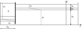
experiments conducted in the large facility are presented here. One experiment in particular, 141010, is chosen for detailed presentation purposes. Figure 1 shows a sketch of the experimental arrangement prior to wave generation. A lower layer was filled first with a prepared solution of brine of prescribed density
 $\unicode[STIX]{x1D70C}_{3}$
(typically
 $1023~\text{kg}~\text{m}^{-3}$
). A top layer was then carefully added via a floating sponge arrangement by directly filling with fresh water of density
 $\unicode[STIX]{x1D70C}_{1}$
(typically
 $998~\text{kg}~\text{m}^{-3}$
). Subsequently, a sharp pycnocline of density
 $\unicode[STIX]{x1D70C}(z)$
, varying as a linear function of depth
 $z$
, formed between the top and bottom layers. Due to practical considerations, the densities
 $\unicode[STIX]{x1D70C}_{1}$
and
 $\unicode[STIX]{x1D70C}_{3}$
varied slightly (
 ${<}0.002\,\%$
) from their prescribed values from run to run. After the layers had been filled, a gate was inserted a distance
 $L_{G}=1.2~\text{m}$
from one end of the tank. The gate was lowered to a depth of approximately
 $2$
cm above the bed of the tank. A prescribed volume
 $V$
of fresh water of density
 $\unicode[STIX]{x1D70C}_{1}$
was then added behind the gate. The fluid in the main section of the tank adjusted itself accordingly such that hydrostatic balance was attained. Once the fluid was completely stationary, the gate was quickly removed and a single ISW of depression was generated, which propagated along the pycnocline into the main section of the tank. By carefully choosing the volume
 $V$
, very-large-amplitude breaking ISWs could be generated (Fructus et al.
Reference Fructus, Carr, Grue, Jensen and Davies2009). Rigid plates of polystyrene were placed on the surface of the water to reduce spurious disturbances and aid comparison with the numerical study.
Schematic diagram of the laboratory arrangement.

For reference purposes, a Cartesian coordinate system
 $(x,y,z)$
, was chosen so that the
 $x$
and
 $z$
directions denoted respectively the horizontal direction of wave propagation and the vertical direction antiparallel to the gravitational acceleration vector
 $\boldsymbol{g}=(0,0,-g)$
. To aid comparison with numerical measures computed in a frame of reference moving with the wave, the origin was chosen such that
 $x=0$
coincided with the trough of the wave and
 $z=0$
coincided with the lower solid boundary of the water column.
2.2 Flow measurement and flow visualisation
An array of high-precision microconductivity sensors was used to measure density profiles (Munro & Davies Reference Munro and Davies2009). The sensors were located at a fixed position in the downstream end of the tank. They were mounted on a motorised rigid rack-and-pinion traverse system fitted with a potentiometer. The sensors were calibrated in advance using saline solutions of known density. The sensors were driven rapidly through the fluid (with a typical transit time of approximately
 $1$
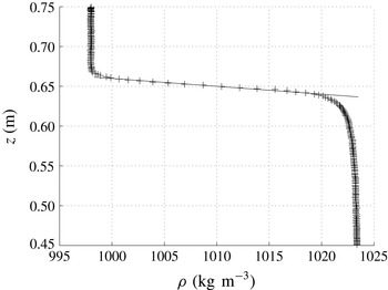
s) to obtain quasi-instantaneous synchronised density profiles in (i) the main section of the tank prior to wave generation and (ii) the breaking part of the wave as the wave propagated along the tank and past the sensors. Figure 2 shows an example of the undisturbed stratification in the main section of the tank, as measured by the sensors. A linear fit was made in the pycnocline region (solid line in figure 2), and the thickness of the pycnocline,
 $h_{2}$
, was defined empirically to be the vertical extent
 $h_{2}$
over which the measured profile satisfied this linear fit (
 $h_{2}=0.02~\text{m}$
in figure 2). The points at which the measured profile deviated by more than
 $1\,\%$
from the linear fit were used to define the thicknesses of the upper and lower layers,
 $h_{1}$
and
 $h_{3}$
respectively. The total fluid depth
 $H$
, in the main section of the tank, was measured with a rule and defined to be
 $H=h_{1}+h_{2}+h_{3}$
.
An example of the stratification in the main section of the tank prior to wave generation. Data points measured by the conductivity sensors are depicted by (
 $+$
) and the solid line is a linear fit to the pycnocline region.

A vertical section in the midplane of the tank was illuminated by a continuous narrow collimated light sheet from an array of light boxes placed below the (transparent) base of the tank. The water column was seeded with neutrally buoyant light-reflecting tracer particles of ‘Pliolite’, having diameters in the range
 $500{-}700~\unicode[STIX]{x03BC}\text{m}$
. It should be noted that, in practice, a given sample of Pliolite contained particles having a range of densities; this property is useful when seeding the fluid as it permits the suspension of tracer particles throughout much of the stratified portion of the water column. In addition, the particles were soaked in a wetting agent prior to use. The amount of time that the particles were soaked for also influenced the range of neutral buoyancy (Grue et al.
Reference Grue, Jensen, Rusås and Sveen1999). The particles here had a buoyancy range that ensured that they were neutrally buoyant throughout the pycnocline, but most tended to coalesce at the top and bottom of the pycnocline (where the fluid density gradient is the highest). This resulted in a higher mean intensity in this illuminated portion than elsewhere. The motions of the tracer particles within the vertical light sheet were viewed and recorded from the side using three fixed digital video cameras set up outside the tank. The cameras were positioned level with the pycnocline to minimise distortion and perspective errors in this portion of the flow field. After each experiment was performed, a perspex grid with reference coordinates was submerged and recorded. This enabled dimensions to be added to the visual images and optical distortions in the processed images to be minimised. Each of the cameras recorded frame images of typical dimensions
 $\unicode[STIX]{x0394}x\approx 0.63~\text{m}$
by
 $\unicode[STIX]{x0394}z\approx 0.45~\text{m}$
, and, in the majority of runs, the cameras were positioned throughout the length of the tank at horizontal distances of
 $4.2$
,
 $7.0$
and
 $9.1~\text{m}$
from the gate. The sensor traverse system was always positioned within the field of view of the most downstream camera such that the density profiles could be associated with flow features seen in the flow visualisation data.
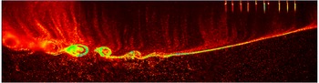
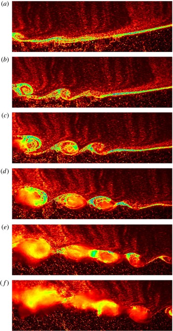
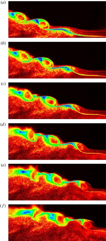
In some instances, the cameras were positioned to have overlapping fields of view and to be synchronised in time. In these cases, it was possible to construct a composite image of the wave over a longer horizontal extent and establish a qualitative view in the wave frame of reference. Figure 3 shows such an experimental image. Light intensity is attributed to light scattered from the particles seeded within the flow and is displayed by a false colour scheme. The wave is travelling from left to right. The composite image in figure 3 provides a representative qualitative view of the breaking dynamics seen in the experiments. Typically, evidence of instability was seen at or close to the wave trough in the form of a small wave on the pycnocline. To the rear of this, KH-like billows developed and subsequently collapsed (sometimes pairing or engulfing/entraining one another in the process). These findings are consistent with those of Fructus et al. (Reference Fructus, Carr, Grue, Jensen and Davies2009) and were seen over the entire experimental data set. The vertical streaks in the upper layer are due to uneven seeding and are not artefacts of the flow dynamics. For completeness, the sequential development of overturning billows in the laboratory frame of reference for the same experiment as in figure 3 is given in figure 4 from the centrally positioned camera.
Side view false colour image showing light intensity from experiment 141010. The horizontal extent of the image is
 $\unicode[STIX]{x0394}x=1.81~\text{m}$
(
 $\unicode[STIX]{x0394}x/H=2.40$
) and the vertical extent is
 $\unicode[STIX]{x0394}z=0.42~\text{m}$
(
 $\unicode[STIX]{x0394}z/H=0.56$
). Conductivity sensors are shown at rest at the top right of the frame.

Still images from experiment 141010. The images are ordered sequentially in time from (a) to (f). Each field of view has a horizontal extent of
 $\unicode[STIX]{x0394}x=0.64~\text{m}$
(
 $\unicode[STIX]{x0394}x/H=0.85$
) and a vertical extent of
 $\unicode[STIX]{x0394}z=0.2~\text{m}$
(
 $\unicode[STIX]{x0394}z/H=0.26$
). The time interval between images is
 $\unicode[STIX]{x0394}t=0.6$
s (
 $c\unicode[STIX]{x0394}t/H=0.16$
).

The video records of the flow field were processed using the software package DigiFlow (Dalziel et al.
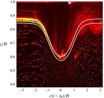
Reference Dalziel, Carr, Sveen and Davies2007). The time series function in DigiFlow was used to monitor the development of the interface by tracking the changes with time of the pixel values in a given column of digitised images extracted from the camera record (see, for example, figure 5). Estimates of the wave amplitude and the time at which the interface reached maximum displacement were then derived from the time series using DigiFlow. The interface location was determined directly from the microconductivity sensors and the visual images analysed at the appropriate trace depths. The amplitudes of the top and the bottom of the pycnocline were taken to be the maximum displacements of the upper and lower isopycnals of the pycnocline respectively. The upper and lower isopycnals of the pycnocline were assumed to have undisturbed depths in the water column of
 $(h_{3}+h_{2})$
and
 $h_{3}$
respectively. This process was repeated at three fixed locations
 $x_{1,2,3}$
over known horizontal distances
 $\unicode[STIX]{x0394}x\approx 0.41H$
(where
 $H=0.75~\text{m}$
on average) on any given camera. This enabled average values for the upper amplitude,
 $a_{u}$
, and lower amplitude,
 $a_{l}$
, to be calculated. Moreover, an estimate of the wave speed
 $c~(=\unicode[STIX]{x0394}x/\unicode[STIX]{x0394}t)$
was obtained by recording the average time
 $\unicode[STIX]{x0394}t$
between maximal interface displacements at the three fixed locations
 $x_{1,2,3}$
. The variances in measuring the wave amplitude and wave speed were
 $3\,\%$
and
 $5\,\%$
respectively.
Time series of vertical variations in pixel intensity for a fixed horizontal position. The reference time
 $t_{0}$
is chosen so that the wave trough is at
 $c(t-t_{0})/H=0$
. The background colour scheme is light intensity from experiment 141010. The solid white curves are the numerical upper and lower traces of the pycnocline, as detailed in § 3.5.

3 Numerical method
3.1 Governing equations
To model numerically the breaking motion of an ISW, the inviscid incompressible Oberbeck–Boussinesq equations in two dimensions were used:
 $$\begin{eqnarray}\displaystyle & \displaystyle \unicode[STIX]{x1D70C}_{0}\left(\boldsymbol{u}_{t}+\boldsymbol{u}\boldsymbol{\cdot }\unicode[STIX]{x1D735}\boldsymbol{u}\right)=-\unicode[STIX]{x1D735}p+\unicode[STIX]{x1D70C}\boldsymbol{g}, & \displaystyle\end{eqnarray}$$
 $$\begin{eqnarray}\displaystyle & \displaystyle \unicode[STIX]{x1D70C}_{t}+\boldsymbol{u}\boldsymbol{\cdot }\unicode[STIX]{x1D735}\unicode[STIX]{x1D70C}=0, & \displaystyle\end{eqnarray}$$
 $$\begin{eqnarray}\displaystyle & \displaystyle \unicode[STIX]{x1D735}\boldsymbol{\cdot }\boldsymbol{u}=0, & \displaystyle\end{eqnarray}$$
where
 $\unicode[STIX]{x1D70C}_{0}$
is a convenient constant reference density (taken here to be the density
 $\unicode[STIX]{x1D70C}_{3}$
in the lower layer),
 $\boldsymbol{u}=(u,w)$
is the fluid velocity vector,
 $t$
denotes time,
 $\unicode[STIX]{x1D735}=(\unicode[STIX]{x2202}/\unicode[STIX]{x2202}x,\unicode[STIX]{x2202}/\unicode[STIX]{x2202}z)$
is the gradient operator,
 $p$
is the fluid pressure and
 $\unicode[STIX]{x1D70C}$
is the fluid density. Buoyancy and vorticity are introduced as
 $b=-g(\unicode[STIX]{x1D70C}-\unicode[STIX]{x1D70C}_{3})/\unicode[STIX]{x1D70C}_{3}$
and
 $\unicode[STIX]{x1D701}=v_{x}-u_{z}$
respectively. Then, taking the curl of the momentum equation (3.1) and rewriting (3.1) and (3.2) in terms of vorticity and buoyancy gives
 $$\begin{eqnarray}\displaystyle & \displaystyle \unicode[STIX]{x1D701}_{t}+\boldsymbol{u}\boldsymbol{\cdot }\unicode[STIX]{x1D735}\unicode[STIX]{x1D701}=b_{x}, & \displaystyle\end{eqnarray}$$
 $$\begin{eqnarray}\displaystyle & \displaystyle b_{t}+\boldsymbol{u}\boldsymbol{\cdot }\unicode[STIX]{x1D735}b=0, & \displaystyle\end{eqnarray}$$
 $$\begin{eqnarray}\displaystyle & \displaystyle \unicode[STIX]{x1D735}\boldsymbol{\cdot }\boldsymbol{u}=0. & \displaystyle\end{eqnarray}$$
To study the evolution of an ISW satisfying (3.4)–(3.6), a numerical iterative procedure was first employed to find a steady-state solution (see King, Carr & Dritschel (Reference King, Carr and Dritschel2010) and § 3.2). The combined Lagrangian advection method (CLAM) was then used to evolve the steady-state solution in time (see Dritschel & Fontane (Reference Dritschel and Fontane2010) and § 3.3).
The computational domain was chosen to be
 $2\unicode[STIX]{x03C0}$
periodic in the horizontal
 $x$
direction and bounded above and below by rigid boundaries at
 $z=0$
and
 $z=L_{z}$
. The aspect ratio of the domain,
 $L_{z}/2\unicode[STIX]{x03C0}$
, was chosen to be
 $0.05$
throughout the study. The domain was, therefore, long compared with the length of the waves, thereby ensuring insignificant effects of periodicity. The ISW was located initially in the centre of the domain.
3.2 The steady-state solver
By noting that buoyancy is conserved along streamlines and that Bernoulli’s theorem holds, the steady-state form of equations (3.4)–(3.6) can be reduced to a simpler form (see King et al. (Reference King, Carr and Dritschel2010) for more details),
 $$\begin{eqnarray}\unicode[STIX]{x1D701}=\unicode[STIX]{x1D735}^{2}\unicode[STIX]{x1D713}=-\frac{N^{2}(Z)}{c^{2}}\unicode[STIX]{x1D713},\end{eqnarray}$$
where
 $\unicode[STIX]{x1D713}(x,z)$
is the streamfunction, defined such that
 $w=\unicode[STIX]{x1D713}_{x}$
and
 $u=-\unicode[STIX]{x1D713}_{z}$
,
 $c$
is the wave speed and
 $N(Z)$
is the buoyancy frequency, defined by
 $$\begin{eqnarray}N^{2}(Z)=\frac{\text{d}\bar{b}}{\text{d}Z}=-\frac{g}{\unicode[STIX]{x1D70C}_{3}}\frac{\text{d}\bar{\unicode[STIX]{x1D70C}}}{\text{d}Z},\end{eqnarray}$$
where bars denote background (or far-field) variables and
 $Z$
is a mass-following coordinate, which effectively traces streamlines.
Solutions of (3.7) for a given
 $N^{2}(Z)$
were computed using an iterative procedure (King et al.
Reference King, Carr and Dritschel2010). First, a uniform computational grid was set up within the domain. The numbers of grid points in the horizontal and vertical directions were
 $n_{x}=1024$
and
 $n_{z}=128$
respectively. The background buoyancy field,
 $\bar{b}(Z)$
, was then found by integrating a given profile of
 $N^{2}(Z)$
with respect to
 $Z$
. The iterative solution procedure was then started with an estimate for
 $\unicode[STIX]{x1D713}$
. A weakly nonlinear solitary wave solution (which is known to be accurate at small wave amplitudes) was used for this purpose. The wave amplitude was defined as
 ${\mathcal{A}}=\unicode[STIX]{x1D702}_{rms}=\unicode[STIX]{x1D713}_{rms}/c$
, where
 $\unicode[STIX]{x1D702}$
is the (downward) streamline displacement and r.m.s. denotes the root-mean-square value. By using the wave speed
 $c_{wnl}$
from the weakly nonlinear solution, an initial amplitude
 ${\mathcal{A}}_{0}=\unicode[STIX]{x1D713}_{rms}/c_{wnl}$
was found. This initial guess was then corrected by solving
 $$\begin{eqnarray}Z=z+\frac{\unicode[STIX]{x1D713}(x,z)}{c}\end{eqnarray}$$
for the isopycnal coordinate
 $Z$
, followed by (3.7) for the vorticity,
 $\unicode[STIX]{x1D701}$
, at each point in the domain (using the previous guess for
 $\unicode[STIX]{x1D713}$
on the right-hand side of (3.7)). Spectral inversion of
 $\unicode[STIX]{x1D6FB}^{2}\unicode[STIX]{x1D713}=\unicode[STIX]{x1D701}$
provided an updated value for
 $\unicode[STIX]{x1D713}$
and
 $$\begin{eqnarray}c=\frac{\unicode[STIX]{x1D713}_{rms}}{{\mathcal{A}}}\end{eqnarray}$$
provided an updated value for
 $c$
. This process was then repeated, by solving (3.9), (3.7) and (3.10), until
 $\unicode[STIX]{x1D713}$
converged. Subsequent states were found for higher amplitudes by increasing
 ${\mathcal{A}}$
in increments of
 $\unicode[STIX]{x1D6FF}{\mathcal{A}}=0.001$
. In this way, for a given background stratification, the parameter space of waves with progressively increasing amplitude was swept. The scheme was stopped once the wave filled half of the domain horizontally. Such large waves exhibit broadening and limit to the conjugate flow discussed in Lamb & Wan (Reference Lamb and Wan1998) and Grue et al. (Reference Grue, Jensen, Rusås and Sveen2000).
3.3 The unsteady solver
To study the evolution of an ISW satisfying (3.4)–(3.6), the numerical procedure outlined in Dritschel & Fontane (Reference Dritschel and Fontane2010) was utilised. It should be noted that no perturbations (or noise components) were added to the steady state. Equation (3.4) for the vorticity was solved using CLAM, a combination of contour advection (Dritschel & Ambaum Reference Dritschel and Ambaum1997) and a pseudospectral method, whereas the conservation equation for the buoyancy (3.5) was solved using contour advection alone to avoid spurious overshoots and undershoots arising from grid-based calculations. The vorticity source
 $b_{x}$
in (3.4) was found directly from the contours used to represent
 $b$
. Since
 $b$
is piecewise uniform,
 $b_{x}$
has the form of a Dirac delta distribution normal to each contour. To obtain
 $b_{x}$
at grid points for use in (3.4), each contour segment between two nodes was divided into 16 equal portions. The source arising from each portion
 $m$
was averaged over the grid box containing the centre of each portion, giving
 $-\unicode[STIX]{x0394}b(z_{m+1}-z_{m})/\unicode[STIX]{x0394}A_{g}$
, where
 $\unicode[STIX]{x0394}b$
is the buoyancy jump across each contour,
 $z_{m+1}-z_{m}$
is the difference in
 $z$
, and
 $\unicode[STIX]{x0394}A_{g}$
is the area of the grid box. Finally, this source was partitioned among the four corners of the grid box using the standard area weights in bilinear interpolation. For high accuracy, this procedure was carried out on a grid four times finer than the ‘inversion’ grid used to solve (3.4). Successive 1–2–1 averages were used to coarsen the source to the inversion grid. Temporal integration was performed using an adaptive fourth-order Runge–Kutta integration scheme. Further details of the method can be found in Dritschel & Fontane (Reference Dritschel and Fontane2010).
3.4 Initialisation of the numerical method
To initialise the numerical simulations, a smooth representation of the stratification measured in the experiments was used. It should be noted that, by rescaling time, the maximum value of the squared buoyancy frequency
 $N^{2}(Z)$
was set to unity in the numerical code. It should also be noted that
 $N^{2}$
was zero in the upper and lower layers since they were homogeneous. Hence, to match
 $N^{2}(Z)$
to the three-layer stratification used in the experiment, the following smooth function was used:
 $$\begin{eqnarray}N^{2}(Z)=\frac{1}{2}\text{erf}\left(\frac{Z-h_{3}}{\unicode[STIX]{x1D6FF}}\right)-\frac{1}{2}\text{erf}\left(\frac{Z-(h_{2}+h_{3})}{\unicode[STIX]{x1D6FF}}\right),\end{eqnarray}$$
where
 $\text{erf}$
denotes the error function and
 $\unicode[STIX]{x1D6FF}$
represents the distance over which the profile was smoothed (typically two numerical grid lengths in
 $z$
). A least squares best fit was then used, with three fitting parameters, namely
 $\unicode[STIX]{x1D6FF}$
,
 $h_{2}$
and
 $h_{3}$
, to obtain a best fit profile of
 $N^{2}(Z)$
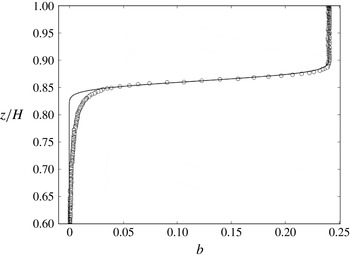
to be used in the numerical simulation. In practice, the fit was applied to the buoyancy profile. A characteristic example from experiment 141010 is given in figure 6.
An example of the undisturbed buoyancy profile (141010). The circles are data points measured by the conductivity probes and the solid line is the analytical line of best fit as described in the text.

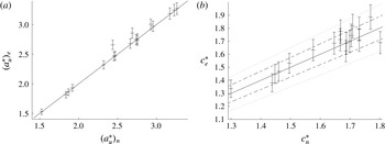
(a) The experimentally measured non-dimensional upper amplitude
 $(a_{u}^{\ast })_{e}$
versus the computed non-dimensional upper amplitude
 $(a_{u}^{\ast })_{n}$
. The solid black line represents
 $(a_{u}^{\ast })_{e}=(a_{u}^{\ast })_{n}$
. (b) The experimentally measured non-dimensional wave speed
 $c_{e}^{\ast }$
versus the computed non-dimensional wave speed
 $c_{n}^{\ast }$
. The dashed and dotted lines respectively represent a deviation of
 $5\,\%$
or
 $10\,\%$
either side of the solid line
 $c_{e}^{\ast }=c_{n}^{\ast }$
.

3.5 Selection of the steady state
Once the buoyancy field was matched, the steady-state solver was run and a spectrum of solutions was found at increasing amplitudes. To find the steady solution that most closely matched the laboratory wave, the amplitude based on the displacement of the upper isopycnal of the pycnocline, namely
 $a_{u}$
, non-dimensionalised by the thickness of the top two layers,
 $h_{1}+h_{2}$
, was given as a target amplitude. The increment in non-dimensional amplitude was free to vary, and as a result it was possible to find a state that closely matched the observed wave. Validation of this matching procedure is given in figures 5 and 7. Figure 5 is a plot of non-dimensional height
 $z/H$
against non-dimensional time
 $c(t-t_{0})/H$
for a specific experiment, 141010, where
 $t_{0}$
has been chosen so that the wave trough is at
 $c(t-t_{0})/H=0$
. The background colour scheme is light intensity from an experimental time series trace of the pycnocline. The solid white curves are numerical traces of the top and bottom of the steady-state pycnocline. It can be seen that in the front part of the wave (negative non-dimensional time), the match between the experimental and numerical wave shapes is very good. The divergence in the rear (positive non-dimensional time) is due to instability in the experimentally generated wave. The agreement between the numerical and experimental traces of the upper isopycnal of the pycnocline is excellent. It is possible to improve the match on the lower isopycnal of the interface by choosing a different steady state, but this comes at the expense of the match on the upper isopycnal. Both the state that gave the best match on
 $a_{u}^{\ast }=a_{u}/(h_{1}+h_{2})$
and the state that gave the best match on
 $a_{l}^{\ast }=a_{l}/(h_{1}+h_{2})$
are used when comparing laboratory and numerical billow characteristics in § 4.2.
In figure 7(a), the level of agreement between the experimentally measured upper amplitude (with an error bar of
 $3\,\%$
) and the purposely matched numerical computation can be seen over the entire data set. Data points represent a given run. Agreement could be improved so that an exact match occurred in every case by simply refining the increment in amplitude that is set when the steady states are computed. Given, however, that the agreement is as good as it is with the increment in non-dimensional amplitude set to a constant value of
 $\unicode[STIX]{x1D6FF}{\mathcal{A}}=0.001$
across the full data set, it was not deemed necessary to vary it from run to run.
Figure 7(b) shows a plot of the experimentally measured non-dimensional wave speed
 $c_{e}^{\ast }=(c/c_{0})_{e}$
(with an error bar of
 $5\,\%$
) versus the computed non-dimensional wave speed
 $c_{n}^{\ast }=(c/c_{0})_{n}$
(computed for the state matched on
 $a_{u}^{\ast }$
), where
 $c_{0}$
, the linear long-wave speed is given by
 $$\begin{eqnarray}c_{0}=\sqrt{\frac{g(\unicode[STIX]{x1D70C}_{3}-\unicode[STIX]{x1D70C}_{1})(h_{3}+h_{2}/2)(h_{1}+h_{2}/2)}{\unicode[STIX]{x1D70C}_{3}H}}.\end{eqnarray}$$
The solid black line represents
 $c_{e}^{\ast }=c_{n}^{\ast }$
, and the dashed and dotted lines respectively represent a deviation of
 $5\,\%$
or
 $10\,\%$
either side of this. The agreement between the two wave speed measures is very good, and, as indicated earlier, it could be refined further by improving the match on
 $a_{u}^{\ast }$
if desired.
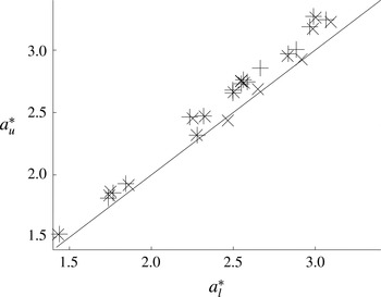
In figure 8, the non-dimensional upper amplitude
 $a_{u}^{\ast }$
versus the non-dimensional lower amplitude
 $a_{l}^{\ast }$
is plotted over the entire data set. Laboratory measurements are denoted by
 $(+)$
and numerically computed data points by
 $(\times )$
. The solid black line represents
 $a_{u}^{\ast }=a_{l}^{\ast }$
. It is clear from this figure that in both the numerical and experimental studies, the upper amplitude measure is consistently larger than the lower amplitude measure, which implies compression of the pycnocline at the wave trough. This is consistent with the field observations of Moum et al. (Reference Moum, Farmer, Smyth, Armi and Vagle2003) and Zhang & Alford (Reference Zhang and Alford2015).
The non-dimensional upper amplitude
 $a_{u}^{\ast }$
versus the non-dimensional lower amplitude
 $a_{l}^{\ast }$
;
 $(+)$
denote laboratory measurements and
 $(\times )$
denote numerically computed data points; the solid line represents
 $a_{u}^{\ast }=a_{l}^{\ast }$
.

4 Results
4.1 Qualitative results and billow interactions
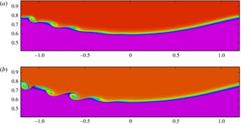
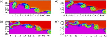
The qualitative agreement between the laboratory observations and numerical simulations can be seen by comparing figure 9 with figure 3. Figure 9 depicts the buoyancy field simulated by the time-dependent numerical code. In this figure, the steady-state waves used to initialise the simulations had (a)
 $a_{l}^{\ast }$
and (b)
 $a_{u}^{\ast }$
chosen to match that of the laboratory wave depicted in figure 3. The buoyancy fields are displayed at times when the flow features looked qualitatively like those in the laboratory. The flow is evolving with time, and a direct quantitative comparison in time cannot be made, as the laboratory and numerical waves are initiated differently.
The numerically computed buoyancy fields obtained by matching (a)
 $a_{l}^{\ast }$
and (b)
 $a_{u}^{\ast }$
to the laboratory experiment depicted in figure 3. The horizontal and vertical axes are
 $x/H$
and
 $z/H$
respectively.

The laboratory experiments showed evidence of billows appearing to evolve independently of each other, and, in addition, examples were seen where individual billows (i) paired with neighbouring billows, (ii) engulfed/entrained each other and (iii) failed to completely overturn. A combination of these different behaviours was sometimes seen on a wave as it propagated along the tank. In the numerical simulations, evolution was observed over a longer time scale, and in these cases, a combination of the behaviours was often seen at different locations relative to the wave trough.
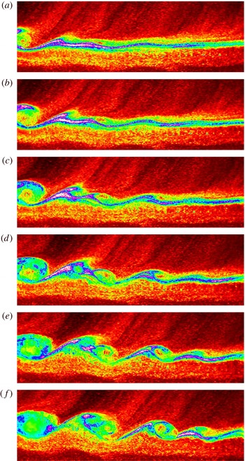
Time sequence of still images from experiment 061010. The images are ordered sequentially from (a) to (f). Each field of view has a horizontal extent of
 $\unicode[STIX]{x0394}x=0.64~\text{m}$
(
 $\unicode[STIX]{x0394}x/H=0.91$
) and a vertical extent of
 $\unicode[STIX]{x0394}z=0.20~\text{m}$
(
 $\unicode[STIX]{x0394}z/H=0.28$
). The time interval between images is
 $\unicode[STIX]{x0394}t=0.3$
s (
 $c\unicode[STIX]{x0394}t/H=0.091$
).

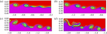
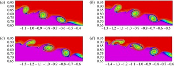
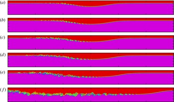
In figure 10, an example of billows pairing in the laboratory can be seen. The panels in figure 10 are ordered sequentially from (a) to (f). The wave is travelling from left to right. On the left of the panels, a billow can be seen that grows alone in time. To the right of this billow, however, two small billows form, which subsequently pair and form one coherent billow. In figure 11, the numerically simulated buoyancy field for the same experiment as in figure 10 is shown. The panels are plotted over the same horizontal and vertical extent as figure 10 and have been chosen in time to show similar pairing characteristics to those observed in the laboratory. The panels in figure 11 are computed in the wave frame of reference, and the limits on the axis differ from frame to frame in order to see how the billows of interest evolve in time. The two billows located at
 $x/H\approx -0.75$
and
 $x/H\approx -0.59$
in figure 11(a) are seen later in their evolution at
 $x/H\approx -1.1$
and
 $x/H\approx -0.99$
in figure 11(b). They subsequently pair in figure 11(c), but start to collapse in figure 11(d) without forming a single coherent billow – a behaviour observed in the laboratory experiment for these conditions.
Time sequence (a)–(d) showing the computed buoyancy field from experiment 061010. The image axes are
 $\unicode[STIX]{x0394}x/H$
and
 $\unicode[STIX]{x0394}z/H$
in the horizontal and vertical directions respectively. The time interval between images is
 $c\unicode[STIX]{x0394}t/H=0.425$
.

In figure 12, an example from the laboratory in which billows engulf and entrain one another is given. It can be seen that, as the flow evolves, the billow initially at the left-hand side of the frame of view engulfs its immediate neighbour to the right (alternatively, the neighbour can be thought of as entraining the billow to its left), and subsequently the billow to the right of that is engulfed also. It should be noted that this behaviour is different from the ‘leap-frog’ instability described by Pawlak & Armi (Reference Pawlak and Armi1998) for a spatially accelerating shear layer. In the leap-frog instability, a billow separates from the primary density interface and skips over a second vortex before interacting with a third or fourth vortex upstream. The crucial difference here is that billows do not separate from the density interface. In figure 13, the corresponding numerical simulation is shown. The dynamics does not appear to be as energetic or turbulent as in the laboratory although the billow at the left-hand edge of the field of view clearly deforms its neighbour to the right as the flow evolves. It should be noted that the discrepancies between the laboratory observations and the numerical simulations are attributed here to 3D effects being present in the laboratory and to differences in the relevant Reynolds numbers in the two cases (see § 4.2.2).
Time sequence of still images from experiment 121010. The images are ordered sequentially from (a) to (f). Each field of view has a horizontal extent of
 $\unicode[STIX]{x0394}x=0.64~\text{m}$
(
 $\unicode[STIX]{x0394}x/H=0.86$
) and a vertical extent of
 $\unicode[STIX]{x0394}z=0.20~\text{m}$
(
 $\unicode[STIX]{x0394}z/H=0.27$
). The time interval between images is
 $\unicode[STIX]{x0394}t=0.3$
s (
 $c\unicode[STIX]{x0394}t/H=0.090$
).

Time sequence (a)–(d) showing the computed buoyancy field from experiment 121010. The image axes are
 $\unicode[STIX]{x0394}x/H$
and
 $\unicode[STIX]{x0394}z/H$
in the horizontal and vertical directions respectively. The time interval between images is
 $c\unicode[STIX]{x0394}t/H=0.122$
.

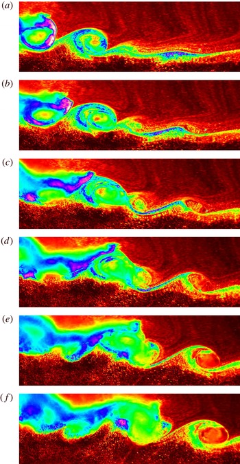
In figure 14, an unusual example from the laboratory is shown in which billows cease to overturn and subsequently collapse. The billow initially at the left-hand edge of the field of view clearly stops overturning with time, and its immediate neighbour to the right appears to show similar characteristics in (f). The corresponding numerical simulation is given in figure 15. Close inspection of the leftmost billow reveals that some isopycnals within the pycnocline (blue, for example) do not accomplish a complete overturn.
Time sequence of still images from experiment 220910. The images are ordered sequentially from (a) to (f). Each field of view has a horizontal extent of
 $\unicode[STIX]{x0394}x=0.65~\text{m}$
(
 $\unicode[STIX]{x0394}x/H=0.87$
) and a vertical extent of
 $\unicode[STIX]{x0394}z=0.24~\text{m}$
(
 $\unicode[STIX]{x0394}z/H=0.32$
). The time interval between images is
 $\unicode[STIX]{x0394}t=0.3$
s (
 $c\unicode[STIX]{x0394}t/H=0.084$
).

Time sequence (a)–(d) showing the computed buoyancy field from experiment 220910. The image axes are
 $\unicode[STIX]{x0394}x/H$
and
 $\unicode[STIX]{x0394}z/H$
in the horizontal and vertical directions respectively. The time interval between images is
 $c\unicode[STIX]{x0394}t/H=0.095$
.

Wave amplitude
 $a_{u}^{\ast }=a_{u}/(h_{1}+h_{2})$
, wave steepness
 $s$
, scale ratio
 $r$
, asymmetry
 $\unicode[STIX]{x1D6FC}$
and corresponding interaction observed. For definitions of
 $r$
and
 $\unicode[STIX]{x1D6FC}$
, see § 4.4.

The most appropriate parameters for classifying billow interaction in the laboratory were found to be the wave amplitude
 $a$
and wave steepness
 $s=a\unicode[STIX]{x03C0}/\unicode[STIX]{x1D706}$
, where
 $\unicode[STIX]{x1D706}$
is the wavelength. In table 1, the wave steepness and wave amplitude are given for the four different interactions that were seen in the laboratory, namely pairing, no interaction, engulfment/entrainment and arrest of overturning. The measure of amplitude is the experimentally measured value. It was not possible to measure wavelength accurately in the laboratory as the tail of the wave was unstable; instead, the numerical steady-state value is used in table 1. Wavelength was defined to be the horizontal extent over which the pycnocline deviated by more than
 $1\,\%$
from its undisturbed depth. It is clear from table 1 and figures 4, 10, 12 and 14 that the shape of the wave affects the type of billow interaction that is seen. Typically, pairing was seen in waves that were broader and flatter, and the dynamics was transient in both the laboratory and the numerical simulations. Such waves are rare in the field; see Shroyer, Moum & Nash (Reference Shroyer, Moum and Nash2011) for an example. Comparison of experiments 141010 and 121010 shows that for engulfment/entrainment to occur between billows, as well as the wave being sufficiently steep, it must also be sufficiently large in amplitude. Finally, comparison of 121010 and 220910 shows that, if the wave is steep enough, billow overturning can be arrested, even if the wave is of an amplitude that is comparable to the highly energetic engulfment/entrainment case.

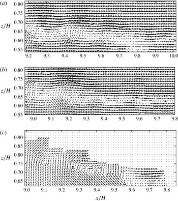
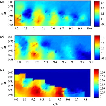
In flat waves, the billows evolve in a near-horizontal flow; see, for example, the particle image velocimetry (PIV) data associated with figure 4(d) (no billow interaction) which are displayed in figure 16(a). In this case, the vertical velocity associated with the ISW is negligible and not strong enough to impede billow overturning (see figure 17(a) for a colour image of the corresponding vertical velocity field scaled by wave speed). In cases where the wave is steep, however, the billows evolve in a flow that has significant variation in the vertical direction; see the PIV data associated with figure 14(a) (arrest of overturning) which are displayed in figure 16(c), for example. In the tail of such steep waves, there is a strong positive vertical velocity field induced by the ISW which opposes the downward side of an overturning billow (see the red regions in the lower portion of figure 17 c). It is conjectured that this wave-induced flow can impede the rotation of a given billow that forms initially near the trough of the wave where the wave-induced vertical velocity is small, and hence prevents its overturning. It should be noted that, due to a lack of seeding in the upper layer of experiment 220910, there are no PIV data in the upper layers of figures 16(c) and 17(c).
Vertical velocity field scaled by measured wave speed
 $c$
for the waves shown in figure 16.

It is noteworthy that asymmetric Holmboe (AH) instabilities never accomplish a complete overturn of the central isopycnal. In some other respects though, they resemble classical KH instabilities (for example, see Carpenter, Lawrence & Smyth (Reference Carpenter, Lawrence and Smyth2007), figures 10(a), 13(a) and 16). All billows observed in this study, however, were KH-like, even those that did not fully overturn (see § 4.4 for more details).
4.2 Quantitative results
4.2.1 Billow speed, billow wavelength and billow growth rate
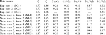
In the experimental observations, it was possible to view and track up to three adjacent billows at a time. To obtain experimental measurements of the billow characteristics, a combination of visual and sensor data was used. First, the density profiles from the sensor measurements and the visual experimental image in the undisturbed portion of the flow field were checked against each other to establish the top and bottom of the pycnocline in the experimental images. When there was good correlation between the two and the pycnocline was easily identified, the visual images were examined using DigiFlow to measure (i) the centre and (ii) the maximum upper and lower extents of given billows. This could be done sequentially in time and, knowing the interval between successive frames and the frame calibration, the values of the billow speed
 $c_{b}$
and billow wavelength
 $\unicode[STIX]{x1D706}_{b}$
could be determined. Billow speed was measured by tracing the distance a billow centre moved (in both the horizontal and vertical directions) in time. Billow wavelength was defined to be the distance from one billow centre to the next. In table 2, average values of billow speed non-dimensionalised by wave speed,
 $c_{b}/c$
, and billow wavelength non-dimensionalised by the thickness of the pycnocline,
 $\unicode[STIX]{x1D706}_{b}/h_{2}$
, are presented for experiment 141010 over the period of measurement. The quantities
 $(c_{b}/c)_{l,m,r}$
denote the speed of the observed left, middle and right billows respectively, and
 $(\unicode[STIX]{x1D706}_{b}/h_{2})_{l,r}$
denote the wavelength measured from the middle billow to its left and right neighbours respectively. The first three rows of data in table 2 are measured values from cameras 1 to 3 respectively.
Average values of billow wave speed and billow wavelength for experiment 141010.

The same procedure was followed in the numerical simulations by probing the computed buoyancy field. In table 2, states 2 and 5 correspond to numerical runs in which the lower (
 $a_{l}^{\ast }$
) and upper amplitudes (
 $a_{u}^{\ast }$
) respectively were matched with the experimental wave. The different trace numbers correspond to different time intervals throughout the numerical simulation in which three adjacent billows were traced. As previously mentioned, the numerical simulations and the laboratory experiment are initiated differently, and in the laboratory the period of observation is much shorter than in the numerical simulations. As such, it is impossible to determine exactly which snapshot of the numerical simulation is most likely to represent the laboratory counterpart. Moreover, in cases where billows interact with one another, measures such as billow speed and billow wavelength vary accordingly. Despite this, the laboratory data in table 2 show excellent agreement with numerical model predictions in the speed of the left billow
 $(c_{b}/c)_{l}$
. There is good agreement in the speed of the middle billow
 $(c_{b}/c)_{m}$
also, but poor agreement in the measure of the right billow
 $(c_{b}/c)_{r}$
. The reason for this systematic discrepancy as the billows are examined from left to right is attributed to the fact that in the laboratory they are observed over diminishing time intervals. The left billow comes into view first, followed by the middle and then the right; the left billow is, therefore, tracked over a longer time interval than the middle billow, which, in turn, is tracked over a longer time than the right billow. The numerically computed wavelength appears to be slightly larger than in the laboratory observations, with the exception of numerical state 2, trace 3, where the agreement is very good.
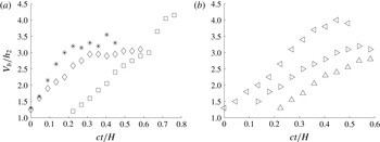
The growth with time of the vertical extent,
 $V_{b}$
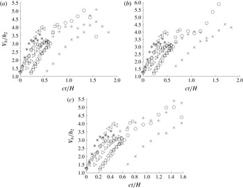
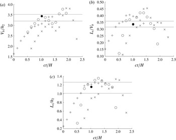
, of a billow is considered in figure 18 for adjacent billows in a given experiment (141010). The billows were tracked from the inception of the left billow until either (i) they collapsed or (ii) they went out of the field of view. Figure 18(a) is taken from camera 1 (EC1). The left (*) and centre (♢) billows are traced until they reach a maximum vertical extent, while the right billow (▫) is traced until it goes out of view, and, in this case, it is still growing in vertical extent. Figure 18(b) is taken from camera 2 (EC2). The left (◃) and centre (▹) billows are traced until just after they have reached a maximum in vertical extent, and the right (▵) until it is just about to attain its maximum.
Plots of
 $V_{b}/h_{2}$
versus dimensionless time
 $ct/H$
for (a) EC1 and (b) EC2. Here, (*, ◃), (♢, ▹) and (▫, ▵) depict the left, middle and right billows respectively in an adjacent set of three.

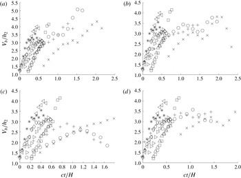
In the numerical simulations (see figures 19 and 20), it is possible to trace the billows over a longer time period. Figures 19 and 20 compare numerical traces (
 $+$
, o,
 $\times$
) with the laboratory traces shown in figure 18 for simulations in which the lower and upper amplitudes respectively were matched with the laboratory measurements. Figures 18–20 all show that, for a given observation (laboratory or simulated), the three billows tracked have a similar growth rate but they attain different maxima in their vertical extent. Figures 19 and 20 show excellent agreement between the simulations and observations for the billow growth rate. The maximum value,
 $V_{bmax}/h_{2}$
, that is attained varies, however, from run to run, and the main difference between figures 19 and 20 is in this measure. Figures 19 and 20 suggest that the larger the amplitude of the wave is (figure 20, as opposed to figure 19), the larger the vertical extent of the billows is (the relationship between wave amplitude and billow height is examined in more detail in § 4.3.1). Figure 19 shows better agreement between the observations and simulations in
 $V_{bmax}/h_{2}$
than figure 20. In all subsequent comparisons, therefore, results from the numerical state 2 (in which the lower amplitude matched the laboratory value) will be used.
Plots of
 $V_{b}/h_{2}$
versus time
 $ct/H$
for (a) EC1, EC2, NL1, (b) EC1, EC2, NL2, (c) EC1, EC2, NL3 and (d) EC1, EC2, NL4. Here, (*, ◃), (♢, ▹) and (▫, ▵) depict the left, middle and right billows respectively in the laboratory observations and (
 $+$
), (○) and (
 $\times$
) depict the left, middle and right billows respectively in the numerical simulation.

Plots of
 $V_{b}/h_{2}$
versus time
 $ct/H$
for (a) EC1, EC2, NU1, (b) EC1, EC2, NU2 and (c) EC1, EC2, NU3. Here, (*, ◃), (♢, ▹) and (▫, ▵) depict the left, middle and right billows respectively in the laboratory observations and (
 $+$
), (○) and (
 $\times$
) depict the left, middle and right billows respectively in the numerical simulation.

4.2.2 Billow heights and vertical displacement scales
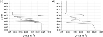
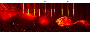
Simultaneous density profiles through a billow were measured in the laboratory by quickly traversing an array of sensors through the tail of the wave as the wave propagated along the tank. Figure 21 shows two such density profiles and figure 22 shows the location of the corresponding sensors used to measure the profiles within the billows. Experimental measurements from the quasi-instantaneous profiles are depicted by the solid line in figure 21. These profiles clearly show evidence of overturning (denser fluid overlying lighter fluid). The degree of overturning within a given billow was assessed by considering the related Thorpe scale (Thorpe Reference Thorpe1977). To do this, the profiles were reordered into monotonically decreasing form, using a bubble sort routine (Dillon Reference Dillon1982). Each data point
 $\unicode[STIX]{x1D70C}_{n}$
initially at a depth
 $z_{n}$
was assigned a new depth
 $z_{m}$
in the reordered profile (dashed line in figure 21). The Thorpe displacement is then defined to be the difference
 $d_{n}^{\prime }=z_{m}-z_{n}$
, with the Thorpe scale
 $L_{T}$
being defined to be the root-mean-square (r.m.s.) of this quantity and
 $L_{Tmax}$
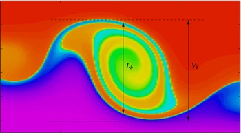
as the maximum Thorpe displacement in a given profile. The vertical extent of the billow through which the sensor travelled was measured visually from the experimental movie and defined to be
 $L_{b}$
. The Thorpe scale was subsequently calculated over this vertical extent. Keller & van Atta (Reference Keller and van Atta2000) and Diamessis & Nomura (Reference Diamessis and Nomura2004) have both shown that inclusion of points with
 $d^{\prime }=0$
can significantly bias the estimate of the average
 $L_{T}$
. It was very rare to have
 $d^{\prime }=0$
; hence, the r.m.s. average was routinely taken over all points in
 $L_{b}$
. Limitations of analysing Thorpe scales from conductivity, temperature and depth (CTD) field data alone are given in van Haren & Gostiaux (Reference van Haren and Gostiaux2014). The Thorpe scales associated with probes (a) and (b) are given in table 3. It should be noted that if the principal axis of the billow in the
 $x$
–
 $z$
plane was horizontal and the sensor struck exactly through the billow centre (as is the case here), then
 $L_{b}=V_{b}$
(i.e the vertical extent over which the Thorpe scale was calculated was equal to the maximal vertical extent of a billow). In cases in which a billow was not orientated horizontally (see, for example, figure 23) or when the sensor did not go through the centre of a billow, then
 $L_{b}$
and
 $V_{b}$
were not equal. Table 3 shows that the (r.m.s.) Thorpe displacement,
 $L_{T}$
, and the maximum Thorpe displacement,
 $L_{Tmax}$
, were approximately
 $34\,\%$
and
 $88\,\%$
of the billow height respectively for the experiment in question.
Depth
 $z$
versus density
 $\unicode[STIX]{x1D70C}$
for sensors (a) and (b) of figure 22. The solid line depicts experimental measurements and the dashed line the sorted profile.

Still image from experiment 141010 showing sensor strikes (a) and (b) in figure 21. The field of view has a horizontal extent of
 $\unicode[STIX]{x0394}x=0.63~\text{m}$
(
 $\unicode[STIX]{x0394}x/H=0.83$
) and a vertical extent of
 $\unicode[STIX]{x0394}z=0.2~\text{m}$
(
 $\unicode[STIX]{x0394}z/H=0.26$
).

An example of a skewed billow in which
 $L_{b}\neq V_{b}$
.

Thorpe data and Reynolds buoyancy number (see text for definition) associated with sensors (a) and (b) and from the numerically simulated middle billow in figure 26. It should be noted that
 $L_{b}=V_{b}$
in all of these cases.

Assuming a linear relationship between the Thorpe scale and the Ozmidov scale, estimates of the turbulent kinetic energy dissipation rate
 $\unicode[STIX]{x1D716}$
can be calculated from the Thorpe scale using the formula
 $\unicode[STIX]{x1D716}=0.64L_{t}^{2}N_{b}^{3}$
(Dillon Reference Dillon1982; Zhang & Alford Reference Zhang and Alford2015), where
 $N_{b}$
is the buoyancy frequency calculated from the sorted profile. This method has been shown to give values of
 $\unicode[STIX]{x1D716}$
within a factor of two of direct oceanographic measurements (MacKinnon & Gregg Reference MacKinnon and Gregg2005; Alford, Gregg & Merrifield Reference Alford, Gregg and Merrifield2006). Recent modelling work (Mater, Schaad & Venayagamoorthy Reference Mater, Schaad and Venayagamoorthy2013) suggests, however, that in strongly stratified flows (i) the relationship between the Thorpe scale and the Ozmidov scale is not linear and (ii) overturns in strongly stratified flows are more indicative of turbulent kinetic energy than dissipation rate. Nonetheless, calculations of
 $\unicode[STIX]{x1D716}$
were made here in order to estimate the Reynolds buoyancy number
 $Re_{b}=\unicode[STIX]{x1D716}/\unicode[STIX]{x1D708}N^{2}$
, where
 $\unicode[STIX]{x1D708}$
is the kinematic viscosity and
 $N$
is taken to be the background buoyancy frequency (calculated from a linear fit of the pycnocline), in order to facilitate comparison with the field measurements of Zhang & Alford (Reference Zhang and Alford2015). A numerical estimate of the viscosity
 $\unicode[STIX]{x1D708}_{num}$
was inferred by noting that a numerical Reynolds number can be defined as
 $Re_{num}=(16L_{y}n/L_{x})^{2}$
, where the characteristic length scale,
 $L_{y}$
, is defined to be the vertical extent of the computational domain and the characteristic dissipation scale is defined to be
 $L_{x}/16n$
, where
 $L_{x}$
is the horizontal extent of the domain and
 $n$
is the number of grid points in the horizontal direction (
 $n=1024$
). Then,
 $\unicode[STIX]{x1D708}_{num}=cL_{y}/Re_{num}$
, where
 $c$
is the computed wave speed. In general, it was found that the laboratory
 $Re_{b}$
was
 $O(10^{2})$
, the numerical values ranged from
 $O(10)-O(10^{3})$
and the field paper of Zhang & Alford (Reference Zhang and Alford2015) suggests a range of
 $O(10^{4})-O(10^{6})$
, making a direct comparison between studies difficult. The billows do, however, appear to be dynamically similar to KH mixing events near the small-scale end of the oceanic range presented in Smyth et al. (Reference Smyth, Moum and Caldwell2001) in which
 $Re_{b}\in [10^{1},10^{4}]$
. While a comparison with the magnitude of the turbulence presented in Zhang & Alford (Reference Zhang and Alford2015) cannot be made, it is clear that the spatial structure of turbulence in Zhang & Alford (Reference Zhang and Alford2015) (see their figure 11 for type I waves) is in keeping with what would be expected from the dynamics seen here, i.e. enhanced regions of dissipation in and around the pycnocline extending from near the trough into the tail.
It was possible to measure Thorpe scales throughout the duration of a simulation. In figure 24, an example is shown of how (a)
 $V_{b}/h_{2}$
, (b)
 $L_{T}/V_{b}$
and (c)
 $L_{T}/h_{2}$
varied with dimensionless time
 $ct/H$
for three adjacent billows from NL2. In these cases,
 $L_{T}$
was calculated over the vertical distance
 $V_{b}$
(calculated directly from buoyancy images). The solid black lines in figure 24 are the experimentally measured values from table 3. As discussed earlier, it is impossible to match instantaneous measurements from the laboratory with computed measures in the simulations as there is no way of identifying unambiguously where the dynamics match those of the laboratory counterpart. It is clear, however, from figure 24 that the simulations capture Thorpe scales that compare favourably with those measured in the laboratory. The level of agreement in figure 24 is typical of that seen throughout the full data set. Figure 24 shows that the non-dimensionalised Thorpe scale varies with time (as the billow grows in vertical extent); this observation is contrary to the findings of De Silva et al. (Reference De Silva, Fernando, Eaton and Hebert1996), who found constant values in parallel shear flow, albeit over a limited number of measurements.
Plots of (a)
 $V_{b}/h_{2}$
, (b)
 $L_{T}/V_{b}$
and (c)
 $L_{T}/h_{2}$
versus dimensionless time
 $ct/H$
from numerical simulation NL2. Here, (
 $+$
), (○) and (
 $\times$
) depict the left, middle and right billow measures respectively in an adjacent set of three. The solid lines and the solid circle are the experimentally measured range and the numerically measured values from table 3 respectively.

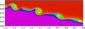
An alternative automated procedure was employed to compute Thorpe scales over the entire horizontal extent of a billow. In these cases, the edge of a billow was defined to be the location where the buoyancy field changed by a prescribed percentage of its maximum or minimum value. The percentage was chosen so that the automated definition of the top and bottom of the undisturbed pycnocline gave the correct pycnocline thickness. The vertical scale over which Thorpe scales were calculated was defined by the vertical separation of the upper and lower billow edges. In figure 25, the simulated buoyancy field for experiment 141010 is presented, with the lower amplitude having been matched with the laboratory-measured value. It should be noted that the billow with centre at
 $x/H\approx -1.12$
is orientated horizontally (i.e the top and bottom of the billow coincide in their
 $x$
location), and, in this case,
 $L_{b}=V_{b}$
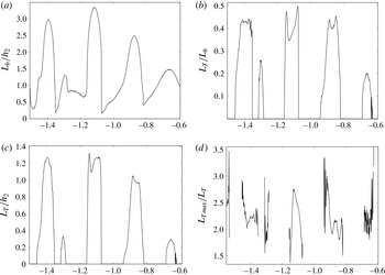
. The Thorpe scale through the centre of this billow at this specific moment in time is given in table 3; the corresponding data points are marked by solid circles in figure 24. The agreement between the laboratory data and the computed data in table 3 is excellent. The horizontal variation in (a)
 $L_{b}/h_{2}$
, (b)
 $L_{T}/L_{b}$
, (c)
 $L_{T}/h_{2}$
and (d)
 $L_{Tmax}/L_{b}$
corresponding to the billows depicted in figure 25 can be seen in figure 26.
The numerically simulated buoyancy field of experiment 141010 at the same dimensionless time
 $ct/H=1.02$
as in figure 24. The vertical and horizontal axes are
 $z/H$
and
 $x/H$
respectively.


4.3 Billow characteristics
The degree of correspondence found between the laboratory observations and the numerical simulations justifies the application of the validated numerical model to sweep parameter space. It should be noted, however, that as the numerical model is inviscid it can only provide meaningful comparison at the larger scales of the overturning motion. In this section, the variations in billow characteristics with (i) wave amplitude and (ii) stratification are examined numerically. For a given wave, the smallest value of amplitude considered was that at which the wave was clearly unstable, while the largest value was limited by the fact that the numerical scheme terminated once the wave filled half of the computational domain horizontally. Many of these large-amplitude cases exhibited the conjugate flow limit behaviour discussed by Lamb & Wan (Reference Lamb and Wan1998); namely, the waves have a maximum vertical displacement at some amplitude and solutions beyond this amplitude simply broaden with a flat central region (the conjugate flow). Previous studies have discussed in detail the effect of wave amplitude and stratification on the onset of instability; see, for example, Fructus et al. (Reference Fructus, Carr, Grue, Jensen and Davies2009), Barad & Fringer (Reference Barad and Fringer2010) and Carr et al. (Reference Carr, King and Dritschel2011). The focus here is on the characteristics of the billows once formed.
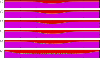
Numerically computed buoyancy field at early time in the simulation for ISWs of amplitude
 $a_{u}^{\ast }=$
(a)
 $1.23$
, (b)
 $1.30$
, (c)
 $1.36$
, (d) 1.42, (e) 1.49 and (f) 1.55 in a stratification in which
 $h_{1}/H=0.19$
,
 $h_{2}/H=0.01$
,
 $h_{3}/H=0.8$
and
 $N_{1}=0=N_{3}$
,
 $N_{2}=1$
. The vertical and horizontal axes are
 $z/H\in [0,1]$
and
 $x/H\in [-6,6]$
respectively.

Numerically computed buoyancy field at midtime in the simulation for the same conditions as figure 27.

4.3.1 Billow dependence on wave amplitude and stratification
Figures 27 and 28 show the numerically computed buoyancy field at early time and midway through the simulation respectively for ISWs of varying non-dimensional amplitude. The stratification was chosen such that the upper, middle and lower layer thicknesses were
 $h_{1}/H=0.19,h_{2}/H=0.01,$
and
 $h_{3}/H=0.8$
respectively, with corresponding buoyancy frequencies of
 $N_{1}=0$
,
 $N_{2}=1$
and
 $N_{3}=0$
respectively. This choice is representative of a linearly stratified pycnocline sandwiched between two homogeneous layers. This replicates the laboratory study and is also representative of what is commonly seen in the ocean (Vlasenko, Stashchuk & Hutter Reference Vlasenko, Stashchuk and Hutter2005). The choice of
 $N_{2}=1$
is somewhat arbitrary due to the way in which the numerical code is non-dimensionalised (see King et al. (Reference King, Carr and Dritschel2010) and Carr et al. (Reference Carr, King and Dritschel2011) for more details). As expected, the waves become broader and flatter with increasing wave amplitude. It should be noted that, at early time (figure 27), the number of billows forming in the pycnocline is dependent on the wave amplitude. However, these billows quickly lose coherence, and, at later times, the number of coherent billows on a wave is independent of the wave amplitude (see figure 28). This trend is seen throughout the data set and is discussed in more detail below (see table 5, for example).


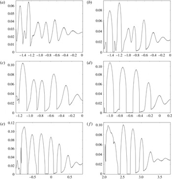
Figure 29 shows the variation with distance
 $x/H$
of the dimensionless vertical extent
 $L_{b}/H$
of the billows. The panels correspond to those in figure 28, and comparison of 29(a–c) implies that the vertical extent of a billow increases with wave amplitude. However, figures 29(d–f) show that once a given amplitude is reached (in this case
 $a_{u}^{\ast }=1.42$
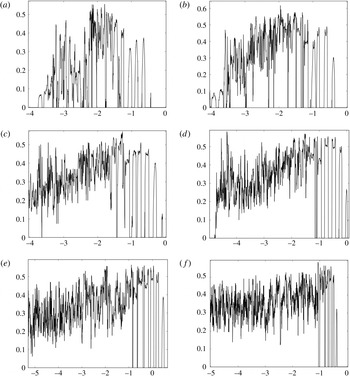
), the measure saturates. This trend is replicated in the corresponding non-dimensional Thorpe scale,
 $L_{T}/L_{b}$
, and is illustrated in figure 30. The maximum value of
 $L_{T}/L_{b}$
in the coherent billows (right hand side of the plots) is approximately
 $0.35,0.45$
and
 $0.5$
in panels (a–c), and thereafter saturates at a value of approximately
 $0.52$
in panels (d–f). De Silva et al. (Reference De Silva, Fernando, Eaton and Hebert1996) reported values of
 $L_{T}/L_{b}\approx 0.49\pm 0.03$
for coherent billows in parallel shear flow, with values of
 $L_{T}/L_{b}\approx 0.29\pm 0.04$
being associated with billows after collapse. Figure 30(d–f) is in excellent agreement with the findings of De Silva et al. (Reference De Silva, Fernando, Eaton and Hebert1996). This is to be expected, as in these cases the waves are increasingly broader and flatter in shape (see figures 27
d–e and 28
d–e); away from the front and rear of the wave, the flow approaches the parallel shear flow configuration. It is interesting to note, however, that the amplitude at which the values of billow height and Thorpe scale saturate is lower than the conjugate flow limit amplitude.


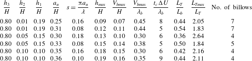
Numerically computed representative billow height, collapse time, Thorpe scale and number of billows. In all cases,
 $N_{1}=0=N_{3}$
and
 $N_{2}=1$
. The lower layer thickness
 $h_{3}$
is fixed.

As for table 4, except that the pycnocline thickness
 $h_{2}$
is fixed.

In table 4, the effect of varying the thickness of the pycnocline,
 $h_{2}$
, on (i) billow height, (ii) time of billow collapse, (iii) Thorpe scale and (iv) the number of coherent billows is shown. The maximum height a billow is expected to achieve in parallel stratified shear flow is given by
 $h_{max}=(\unicode[STIX]{x0394}U)^{2}/\unicode[STIX]{x0394}b$
, where
 $\unicode[STIX]{x0394}U$
and
 $\unicode[STIX]{x0394}b$
are the velocity and buoyancy jumps respectively (see De Silva et al. (Reference De Silva, Fernando, Eaton and Hebert1996) and references therein), and where
 $h_{max}$
is calculated using
 $\unicode[STIX]{x0394}U$
and
 $\unicode[STIX]{x0394}b$
at the wave trough. In the present study, the averaged values of the maximum billow height attained,
 $V_{bmax}$
, and the time of billow collapse,
 $t_{c}$
, were found by tracing a set of three billows midway through a given simulation until signs of deformation in the billow shape were seen. Such measures (and the associated Thorpe scale) were adopted as representative values of these quantities. To count billows consistently, the number of billows on a wave at a given instant in time was found by adding the primary billow just before collapse to those upstream of it. Here, small-scale wave-like disturbances on the pycnocline were included which were known to subsequently roll up at later times. For example, in figure 28, the number of coherent billows would be counted as 7–8. For a given stratification, traces were made of (i) the smallest amplitude unstable wave and (ii) the largest amplitude wave computed. In many cases, these large-amplitude waves approach the conjugate flow limit. Table 4 confirms the findings of Carr et al. (Reference Carr, King and Dritschel2011) that the critical amplitude required for instability decreases with a decrease in pycnocline thickness (cf. the amplitude measures in the first row of each section of table 4). The table suggests that thicker pycnoclines can support larger and, accordingly, fewer billows on a given wave. Care should be taken with this interpretation, however, since the wave amplitude is also varying over the data set.
In fact, the critical parameter controlling the height a billow can attain is the wave amplitude, and it is clear from table 4 that the larger the wave amplitude is, the larger the value of
 $V_{bmax}/H$
is (in keeping with the findings of § 4.3.1). Moreover, the table shows good agreement between the predicted
 $h_{max}/H$
and measured
 $V_{bmax}/H$
values, with agreement, as expected, being best in cases where
 $s=0.08$
(and the waves approach the conjugate flow limit). The agreement implies that the height a billow can attain scales with
 $(\unicode[STIX]{x0394}U)^{2}/\unicode[STIX]{x0394}b$
(rather than
 $h_{2}$
or
 $\unicode[STIX]{x1D706}_{b}$
) over the full range of steepness values investigated. In the parallel shear flow case, De Silva et al. (Reference De Silva, Fernando, Eaton and Hebert1996) found values of
 $V_{bmax}/\unicode[STIX]{x1D706}_{b}\approx 0.40$
and
 $t\unicode[STIX]{x0394}U/\unicode[STIX]{x1D706}_{b}\approx 5$
, and excellent agreement is seen with these values in the two cases where
 $s=0.08$
. The maximum billow height and time of billow collapse vary with
 $s$
, confirming the findings of § 4.1 that wave shape affects the billow characteristics.
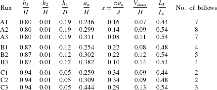
In table 5, the effect of varying the thicknesses of the upper and lower layers while keeping the thickness of the pycnocline fixed is shown. For a given stratification, three different wave amplitudes are shown. In addition to the smallest and largest amplitudes, a fixed value of
 $a_{u}/H\approx 0.3$
(A2, B2, C2) is displayed to allow comparison between the three subsets of data. Amplitude measures are given to three decimal places to show that the results are in keeping with Carr et al. (Reference Carr, King and Dritschel2011), who showed that the critical amplitude required for instability increases with an increase in
 $h_{3}$
(cf. A1, B1 and C1). Table 5 clearly shows that the number of billows decreases as
 $h_{3}$
increases, and at a fixed amplitude (
 $a_{u}/H\approx 0.3$
– A2, B2, C2), an increase in
 $h_{3}$
coincides with the wavelength being shorter (
 $s$
increases but
 $a_{u}$
is fixed). In other words, shorter waves support fewer billows. Moreover, the first two sections of the table (A–B) imply that the height a billow attains increases for shorter waves (cf. A2 and B2). The third section (C) does not confirm the trend, but it should be noted that in this case the presence of the upper boundary restricted the height attainable. In general, it was found that shorter (steeper) waves support fewer but larger billows for a given wave amplitude and pycnocline thickness.
4.4 Kelvin–Helmholtz instability
The billows in this study are Kelvin–Helmholtz (KH)-like and shared the same qualitative characteristics as classical KH overturns associated with parallel shear flow. Moreover, they exhibited quantitative agreement with classical KH billows in several different measures. For example, Smyth et al. (Reference Smyth, Moum and Caldwell2001) found that
 $L_{Tmax}/L_{T}\in [2,3]$
in both simulated KH billows and turbulent patches observed in the ocean thermocline. Figure 26(d) and table 4 are in excellent agreement with this. A linear stability analysis of the Taylor–Goldstein equation yields
 $\unicode[STIX]{x1D706}_{b}/h_{2}=7.5\pm 0.7$
for KH billows in breaking ISWs (see Hazel Reference Hazel1972; Fructus et al.
Reference Fructus, Carr, Grue, Jensen and Davies2009). Table 2 is in very good agreement with this. Moreover, in the numerical results, it is possible to check that the propagation speed of a billow is approximately equal to the mean flow speed at the depth of maximum shear, also a characteristic of KH instability. Finally, as already noted above, it is found that in broad flat waves, the maximum billow height attained and the time of billow collapse are in excellent agreement with the results for KH overturning in parallel shear flow, as documented by De Silva et al. (Reference De Silva, Fernando, Eaton and Hebert1996).
One qualitative exception in the data set was the example in which billow overturning was arrested (see figures 14 and 15). It should be noted that AH instabilities never accomplish a complete overturn of the central isopycnal but otherwise look similar to classical KH instabilities (for example, see Carpenter et al. (Reference Carpenter, Lawrence and Smyth2007), figures 10(a), 13(a) and 16). To distinguish whether an instability is of KH or AH type, a scale ratio
 $r$
and asymmetry factor
 $\unicode[STIX]{x1D6FC}$
can be computed, and are respectively defined to be
 $$\begin{eqnarray}r=\frac{\unicode[STIX]{x0394}u_{z}}{\unicode[STIX]{x0394}\unicode[STIX]{x1D70C}_{z}},\quad \unicode[STIX]{x1D6FC}=\frac{2d}{\unicode[STIX]{x0394}u_{z}},\end{eqnarray}$$
where
 $\unicode[STIX]{x0394}u_{z}$
and
 $\unicode[STIX]{x0394}\unicode[STIX]{x1D70C}_{z}$
are the vertical extent of the velocity shear and pycnocline respectively at the wave trough and
 $d$
is the offset between the centre of the shear layer and the pycnocline. The values of
 $r$
and
 $\unicode[STIX]{x1D6FC}$
calculated for the waves investigated in § 2 are shown in table 1. No discernible difference is seen between the example in which billow overturning was arrested (220910) and the rest of the data set. If anything, the
 $r$
value in this case appears to be lower than the others. This property is contrary to the trend necessary for this case to be an AH instability (which would require a higher
 $r$
value). This further confirms that all billows observed were KH-like.
5 Conclusion and discussion
A combined laboratory and numerical study was made of shear-induced overturning billows associated with unstable ISWs. Examples from the laboratory are given in which billows (i) evolve independently of one another, (ii) pair with each other, (iii) engulf/entrain each other and (iv) have arrested overturning. In the vast majority of cases, the billows fully overturn. One example is given in which billow overturning is arrested before collapsing, and it is conjectured that the wave-induced vertical velocity in the rear of the wave is responsible for this behaviour. Overall, the steepness of the wave and the wave amplitude are found to be the most appropriate parameters for distinguishing between these different billow behaviours.
Numerical simulations are shown to capture accurately the main billow characteristics, including billow speed, billow wavelength, billow growth rate and billow Thorpe scale. When the waves are close to the conjugate flow limit (broad and flat), the billow characteristics are in excellent agreement with those associated with parallel stratified shear flow (De Silva et al. Reference De Silva, Fernando, Eaton and Hebert1996), but when the waves are steeper or shorter, the spatially varying wave-induced shear flow is shown to modify the billow characteristics. In particular, the height that a billow can attain (and its associated Thorpe scale) is dependent primarily on wave amplitude, but the value saturates once a certain amplitude is reached, and interestingly this amplitude is less than the conjugate flow limit amplitude. Moreover, the number of coherent billows that form on a wave is dependent on wavelength, with shorter waves supporting fewer but larger billows than longer waves for a given pycnocline thickness.
This study has been restricted to 2D and to Reynolds numbers significantly less than typical values in the ocean. Geyer et al. (Reference Geyer, Lavery, Scully and Trowbridge2010) showed that KH billows in a stratified estuary are radically different in structure at geophysical Reynolds numbers compared with those studied at smaller
 $Re$
. Moreover, the 3D simulations of Mashayek & Peltier (Reference Mashayek and Peltier2011) have shown that KH billow pairing may be entirely suppressed in parallel stratified shear flow at high Reynolds numbers due to the growth of 3D secondary instabilities. Typically, billow pairing in this study is seen in waves that are broad and flat. Observations of such waves in the ocean are rare (see Shroyer et al. (Reference Shroyer, Moum and Nash2011) for an example), and billow pairing is not expected to be observed in the ocean.
The fastest growing modes in parallel shear flow are 2D modes, and KH instabilities are initially 2D until they saturate and collapse (Peltier & Caulfield Reference Peltier and Caulfield2003). Whether this is the case in ISWs is not known. An understanding of how 2D instabilities in ISWs three-dimensionalise and subsequently affect mixing efficiency is an important open area of future research. Further study is also required to understand what mixing results from ISW breaking and how the stratification behind an unstable ISW is modified.
Acknowledgements
The authors are grateful for support from the UK Engineering and Physical Sciences Research Council (EPSRC) under its Mathematical Sciences Programme (grant no. EP/F030622/1) and the University of Oslo and the Research Council of Norway through NFR191204/V30. J.F. was supported by a PhD studentship funded jointly by the Northern Research Partnership and an EPSRC Doctoral Training Grant. The authors would like to thank Professor J. Duncan and three anonymous referees whose comments led to significant improvements in the paper.