








1 Introduction
When an inclined surface is thermally altered from the state of the overlying fluid, the resulting buoyancy force projects in both the along- and normal-to-slope directions. Surface cooling results in a downslope flow (katabatic flow), whereas surface heating generates an upslope flow (anabatic flow). The significance of such sloping turbulent flows is rarely questioned given their ubiquity and their central role in land–atmosphere exchange processes. Katabatic and anabatic flows are persistent over complex terrains (Whiteman Reference Whiteman1990; Monti et al. Reference Monti, Fernando, Princevac, Chan, Kowalewski and Pardyjak2002; Rampanelli, Zardi & Rotunno Reference Rampanelli, Zardi and Rotunno2004; Haiden & Whiteman Reference Haiden and Whiteman2005; Rotach & Zardi Reference Rotach and Zardi2007; Fernando Reference Fernando2010; Zardi & Whiteman Reference Zardi and Whiteman2013; Nadeau et al. Reference Nadeau, Pardyjak, Higgins, Huwald and Parlange2013a ; Oldroyd et al. Reference Oldroyd, Katul, Pardyjak and Parlange2014, Reference Oldroyd, Pardyjak, Huwald and Parlange2016b ; Fernando et al. Reference Fernando, Pardyjak, Di Sabatino, Chow, De Wekker, Hoch, Hacker, Pace, Pratt and Pu2015; Lehner et al. Reference Lehner, Whiteman, Hoch, Jensen, Pardyjak, Leo, Di Sabatino and Fernando2015; Grachev et al. Reference Grachev, Leo, Sabatino, Fernando, Pardyjak and Fairall2016; Hang et al. Reference Hang, Nadeau, Gultepe, Hoch, Román-Cascón, Pryor, Fernando, Creegan, Leo and Silver2016; Jensen et al. Reference Jensen, Nadeau, Hoch and Pardyjak2016), and despite their local nature, their interaction with larger-scale forcing mechanisms can favour the development of cyclonic vorticity in the middle and upper troposphere (Parish Reference Parish1992; Parish & Bromwich Reference Parish and Bromwich1998). Katabatic winds regulate energy, momentum and mass transfer over the ice sheets of Greenland and Antarctica (Egger Reference Egger1985; Parish Reference Parish1992; Parish & Bromwich Reference Parish and Bromwich1998; Renfrew Reference Renfrew2004; Renfrew & Anderson Reference Renfrew and Anderson2006), and also influence the movement of the marginal ice zone (Chu Reference Chu1987). In addition, katabatic flows are a permanent feature of the atmospheric boundary layer (ABL) over melting glaciers (Greuell et al. Reference Greuell, Broeke Van den, Knap, Reijmer, Smeets and Struijk1994; Smeets, Duynkerke & Vugts Reference Smeets, Duynkerke and Vugts1997; Oerlemans Reference Oerlemans1998; Oerlemans et al. Reference Oerlemans, Björnsson, Kuhn, Obleitner, Palsson, Smeets, Vugts and Wolde1999; Smeets, Duynkerke & Vugts Reference Smeets, Duynkerke and Vugts2000; Parmhed, Oerlemans & Grisogono Reference Parmhed, Oerlemans and Grisogono2004), whose constant retreat is a matter of public interest, given their impact on both the sea level rise and on water resource management.
Prandtl (Reference Prandtl1942) framed the problem of slope flows in a conceptually simple model, considering a doubly infinite (no leading edges) plate that is uniformly heated or cooled and lies within a stably stratified environment. The Prandtl model (Prandtl Reference Prandtl1942) states that the advection of base-state (environmental) potential temperature is balanced by buoyancy (diffusive) flux divergence, whereas the slope-parallel component of buoyancy balances momentum (diffusive) flux divergence. This particular type of flows are termed equilibrium flows (Mahrt Reference Mahrt1982), given the nature of the balance between a turbulent flux divergence and a generation/destruction mechanism. Under such settings, the Boussinesq equations of motion and thermal energy reduce to one-dimensional form, which allows for analytical treatment. Accounting for a base stable stratification admits solutions that approach steady-state conditions at large times, whereas in the absence of a stable stratification (classical solutions), the thermal and dynamic boundary layers (TBL and DBL in the following) grow in an unbounded manner (Menold & Yang Reference Menold and Yang1962).
The original model assumed constant turbulent diffusivities (labelled as K) – and is therefore incapable of representing the observed steep near-surface gradients (Grisogono & Oerlemans Reference Grisogono and Oerlemans2001b ). In addition, the return flow region predicted by the constant-K solution is usually stronger, when compared to measurements or numerical simulations, and also vanishes more rapidly away from the surface (Defant Reference Defant1949; Denby Reference Denby1999; Grisogono & Oerlemans Reference Grisogono and Oerlemans2001b ). This limitation was first overcome in Gutman (Reference Gutman1983), where a patched analytic solution was proposed, valid for linearly decreasing K in the inner flow regions. More recently, Grisogono & Oerlemans (Reference Grisogono and Oerlemans2001b , Reference Grisogono and Oerlemans2002) proposed an approximate analytical solution able to account for gradually varying eddy diffusivities, valid under the WKB approximation (after Wentzel–Kramers–Brillouin), and a closed form solution valid for O’Brien type K was derived in Giometto et al. (Reference Giometto, Grandi, Fang, Monkewitz and Parlange2017). Modifications of the Prandtl model to allow for variations in surface forcing (Shapiro & Fedorovich Reference Shapiro and Fedorovich2007, Reference Shapiro and Fedorovich2008; Burkholder, Shapiro & Fedorovich Reference Burkholder, Shapiro and Fedorovich2009), to account for Coriolis effects (Kavavcic & Grisogono Reference Kavavcic and Grisogono2007; Shapiro & Fedorovich Reference Shapiro and Fedorovich2008), time dependence of the solution (Shapiro & Fedorovich Reference Shapiro and Fedorovich2004, Reference Shapiro and Fedorovich2005, Reference Shapiro and Fedorovich2008; Zardi & Serafin Reference Zardi and Serafin2015) and for weakly nonlinear effects (Grisogono et al. Reference Grisogono, Jurlina, Večenaj and Güttler2014; Güttler et al. Reference Güttler, Marinović, Večenaj and Grisogono2016), were also recently proposed.
The Prandtl conceptual approach is also of interest in numerical modelling. It alleviates computational costs by constraining the geometry to regular domains, thus allowing the use of efficient numerical schemes such as methods based on finite differences or spectral expansions. The existence of a statistically steady-state solution also provides a benchmark for quantitative analysis. The past decades have seen significant advances in computational performance, achieved through both improvements in computer hardware and in numerical algorithms that solve differential equations. Nevertheless, computational cost of simulating high Reynolds number (
 $Re$
) flows over long slopes remains prohibitively high, and has motivated the use of closure models that aim at reducing resolution requirements in the dissipative range, especially when energy-containing scales are of primary interest (Pope Reference Pope2000). Since the pioneering work of Schumann (Reference Schumann1990), large-eddy simulation (LES) has represented one of the workhorses for the simulation of slope flows within the Prandtl model framework. It has revealed several aspects of the turbulent structure and illustrated the sensitivity of the bulk solution to the system parameters (Skyllingstad Reference Skyllingstad2003; Axelsen & Dop Reference Axelsen and Dop2009a
,Reference Axelsen and Dop
b
; Grisogono & Axelsen Reference Grisogono and Axelsen2012). LES of slope flows in more complex configurations (i.e. not relying on the Prandtl model set-up) have been performed in Smith & Skyllingstad (Reference Smith and Skyllingstad2005), where the effects of varying slope angle were analysed, and the interaction of slope flows with valley systems have also been recently addressed via LES (Chow et al.
Reference Chow, Weigel, Street, Rotach and Xue2006; Weigel et al.
Reference Weigel, Chow, Rotach, Street and Xue2006; Chemel, Staquet & Largeron Reference Chemel, Staquet and Largeron2009; Burns & Chemel Reference Burns and Chemel2014, Reference Burns and Chemel2015; Arduini, Staquet & Chemel Reference Arduini, Staquet and Chemel2016). However, the stable stratification and the peculiar features characterizing slope flows (e.g. the presence of zero-gradient layers in the state variables) question the validity of the assumptions upon which LES subgrid-scale (SGS) models are derived (Burkholder, Fedorovich & Shapiro Reference Burkholder, Fedorovich and Shapiro2011). In addition, the lack of a rigorous similarity theory for slope flows (Mahrt Reference Mahrt1998; Grisogono & Oerlemans Reference Grisogono and Oerlemans2001a
; Grisogono, Kraljevic & Jericevic Reference Grisogono, Kraljevic and Jericevic2007; Mahrt Reference Mahrt2013; Nadeau et al.
Reference Nadeau, Pardyjak, Higgins and Parlange2013b
; Monti, Fernando & Princevac Reference Monti, Fernando and Princevac2014; Oldroyd et al.
Reference Oldroyd, Pardyjak, Higgins and Parlange2016a
) makes it impossible to prescribe adequate surface fluxes in simulations. These limitations have motivated the use of direct numerical simulations (DNS), which, despite their modest range of
 $Re$
, provide the most comprehensive view of the flow structure (Fedorovich & Shapiro Reference Fedorovich and Shapiro2009) (FS09 hereafter). These studies showed that slope-flow statistics are sensitive to variations in the parameter space, including the magnitude of the surface forcing, the slope angle and the strength of the ambient stratification. They all play a role in determining the characteristics of the flow. This finding motivated recent efforts towards a derivation of scaling relations that allow the elimination of the dependency of the solution on the sloping angle (Shapiro & Fedorovich Reference Shapiro and Fedorovich2014). Scaling relations are of interest since they facilitate the design of experiments and have potentials to yield significant computational savings in parametric studies when explored through LES and DNS.
In this work, the problem of anabatic and katabatic flows and the properties of the LLJ in the near-wall region are explored using high resolution DNS. The focus is on variations in the slope-normal structure of selected flow statistics and in integrated quantities as a function of the sloping angle (
 $\unicode[STIX]{x1D6FC}$
) and of the Grashof number (
 $Gr$
). The flow is driven by a homogeneous constant surface buoyancy force and the molecular Prandtl number (
 $Pr$
) is set to unity (instead of a typical 0.7 value for air) in line with the FS09 study. The current study complements and extends the work of FS09, where a similar set-up was adopted to characterize slope flows driven by an imposed surface buoyancy flux. The aim is to shed additional light on the interactions between turbulence and the mean flow state as well as the role of the low-level jet (LLJ) in energy and momentum exchanges. Specifically, the study aims at (i) assessing how
 $\unicode[STIX]{x1D6FC}$
and
 $Gr$
influence katabatic and anabatic flows when constant surface buoyancy is prescribed; (ii) contrasting key features between slope flows driven by a constant imposed surface buoyancy, when compared against slope flows generated by a constant imposed surface buoyancy flux; and (iii) characterizing the vertical structures (and their sensitivity to variations in the parameter space) of mean kinetic energy (MKE) and of turbulent kinetic energy (TKE) budget terms. The long-term goal is to provide improvements for current turbulence closure models for sloping and stable conditions that can then be implemented in large-scale atmospheric models so as to address the plethora of problems already highlighted earlier on in the introduction. The manuscript is organized as follows. The governing equations for the problem are derived in § 2. Section 3 provides details on the numerical algorithm and on the set-up of simulations and the main results are presented in § 4. Summary and concluding remarks follow in § 5.
Slope-aligned coordinate system.

2 Equations of motion
Thermal convection of turbulent stratified fluid flow over sloping surfaces can be described in a slope-rotated reference system, where
 $\hat{x}$
is the along-slope direction,
 ${\hat{y}}$
denotes the spanwise direction and
 $\hat{z}$
is the slope-normal direction, as displayed in figure 1.
 $(\hat{\cdot })$
indicates a dimensional variable. The potential temperature
 $\hat{\unicode[STIX]{x1D703}}(\hat{\boldsymbol{x}},\hat{t})$
is decomposed into a base state
 $\hat{\unicode[STIX]{x1D703}}^{R}(\hat{z}^{\ast })$
and a perturbation component
 $\hat{\unicode[STIX]{x1D703}}^{\prime \prime }(\hat{\boldsymbol{x}},\hat{t})\equiv \hat{\unicode[STIX]{x1D703}}(\hat{\boldsymbol{x}},\hat{t})-\hat{\unicode[STIX]{x1D703}}^{R}(\hat{z}^{\ast })$
as originally proposed by Prandtl (Reference Prandtl1942). Assuming the base state
 $\hat{\unicode[STIX]{x1D703}}^{R}(\hat{z}^{\ast })$
to be a linear function of the vertical coordinate direction
 $\hat{z}^{\ast }$
, results in
 $\hat{N}\equiv \sqrt{\hat{\unicode[STIX]{x1D6FD}}(\text{d}\hat{\unicode[STIX]{x1D703}}^{R}/\text{d}\hat{z}^{\ast })}=\text{const.}$
, where
 $\hat{N}$
is the buoyancy frequency (equivalent to the Brunt–Väisälä frequency). The thermal expansion coefficient
 $\hat{\unicode[STIX]{x1D6FD}}\equiv {\hat{g}}/\hat{\unicode[STIX]{x1D703}}_{0}$
where
 ${\hat{g}}$
is the acceleration due to gravity and
 $\hat{\unicode[STIX]{x1D703}}_{0}$
is a reference constant temperature. Moreover, invoking the Boussinesq approximation (i.e. ignoring density differences except where they appear in terms multiplied by
 ${\hat{g}}$
) and neglecting earth rotation effects, the conservation equations within the DBL and TBL in dimensional form reduce to
 $$\begin{eqnarray}\displaystyle & \displaystyle \frac{\unicode[STIX]{x2202}\hat{u} _{i}}{\unicode[STIX]{x2202}\hat{t}}+\frac{\unicode[STIX]{x2202}\hat{u} _{i}\hat{u} _{j}}{\unicode[STIX]{x2202}\hat{x}_{j}}=-\frac{\unicode[STIX]{x2202}\hat{\unicode[STIX]{x03C0}}}{\unicode[STIX]{x2202}\hat{x}_{i}}+\hat{\unicode[STIX]{x1D708}}\frac{\unicode[STIX]{x2202}^{2}\hat{u} _{i}}{\unicode[STIX]{x2202}\hat{x}_{j}^{2}}-\hat{\unicode[STIX]{x1D6FD}}\hat{\unicode[STIX]{x1D703}}^{\prime \prime }(\hat{\boldsymbol{x}},\hat{t})[\unicode[STIX]{x1D6FF}_{i1}\sin \unicode[STIX]{x1D6FC}-\unicode[STIX]{x1D6FF}_{i3}\cos \unicode[STIX]{x1D6FC}], & \displaystyle\end{eqnarray}$$
 $$\begin{eqnarray}\displaystyle & \displaystyle \frac{\unicode[STIX]{x2202}\hat{u} _{i}}{\unicode[STIX]{x2202}\hat{x}_{i}}=0, & \displaystyle\end{eqnarray}$$
 $$\begin{eqnarray}\displaystyle & \displaystyle \frac{\unicode[STIX]{x2202}\hat{\unicode[STIX]{x1D703}}^{\prime \prime }}{\unicode[STIX]{x2202}\hat{t}}+\frac{\unicode[STIX]{x2202}\hat{u} _{j}\hat{\unicode[STIX]{x1D703}}^{\prime \prime }}{\unicode[STIX]{x2202}\hat{x}_{j}}=-\frac{\unicode[STIX]{x2202}\hat{u} _{j}\hat{\unicode[STIX]{x1D703}}^{R}}{\unicode[STIX]{x2202}\hat{x}_{j}}+\hat{\unicode[STIX]{x1D705}}\frac{\unicode[STIX]{x2202}^{2}\hat{\unicode[STIX]{x1D703}}^{\prime \prime }}{\unicode[STIX]{x2202}\hat{x}_{j}^{2}}, & \displaystyle\end{eqnarray}$$
where
 $\hat{t}~(\text{s})$
denotes time,
 $\hat{u} _{i}~(\text{m}~\text{s}^{-1})$
,
 $i=1,2,3$
, are the velocity components in the three coordinate directions
 $(\hat{x},{\hat{y}},\hat{z})\,(\text{m})$
,
 $\hat{\unicode[STIX]{x03C0}}\equiv [\hat{p}-\hat{p}^{R}(\hat{x},\hat{z})]/\hat{\unicode[STIX]{x1D70C}}_{0}\,(\text{m}^{2}~\text{s}^{-2})$
is the normalized deviation of kinematic pressure from the background hydrostatic state,
 $\hat{\unicode[STIX]{x1D70C}}_{0}\,(\text{kg}~\text{m}^{-3})$
is a reference constant density,
 $\unicode[STIX]{x1D6FC}\,(\text{rad})$
is the slope angle,
 $\hat{\unicode[STIX]{x1D708}}\,(\text{m}^{2}~\text{s}^{-1})$
and
 $\hat{\unicode[STIX]{x1D705}}\,(\text{m}^{2}~\text{s}^{-1})$
are the kinematic molecular viscosity and thermal diffusivity coefficients, and
 $\unicode[STIX]{x1D6FF}_{ij}$
is the Kronecker Delta function. Molecular dissipation of kinetic energy represents an additional source of heat, and should in principle be included in the equation for
 $\hat{\unicode[STIX]{x1D703}}$
. However, due to the low velocities involved in slope flows this term is small and has thus been neglected. Introducing the buoyancy variable
 $\hat{b}(\hat{\boldsymbol{x}},\hat{t})\equiv \hat{\unicode[STIX]{x1D6FD}}\hat{\unicode[STIX]{x1D703}}^{\prime \prime }(\hat{\boldsymbol{x}},\hat{t})$
, and since
 $\hat{z}^{\ast }(\hat{\boldsymbol{x}})\equiv -\hat{x}\sin \unicode[STIX]{x1D6FC}+\hat{z}\cos \unicode[STIX]{x1D6FC}$
, equations (2.1)–(2.3) can be re-written as in FS09
 $$\begin{eqnarray}\displaystyle & \displaystyle \frac{\unicode[STIX]{x2202}\hat{u} _{i}}{\unicode[STIX]{x2202}\hat{t}}+\frac{\unicode[STIX]{x2202}\hat{u} _{i}\hat{u} _{j}}{\unicode[STIX]{x2202}\hat{x}_{j}}=-\frac{\unicode[STIX]{x2202}\hat{\unicode[STIX]{x03C0}}}{\unicode[STIX]{x2202}\hat{x}_{i}}+\hat{\unicode[STIX]{x1D708}}\frac{\unicode[STIX]{x2202}^{2}\hat{u} _{i}}{\unicode[STIX]{x2202}\hat{x}_{j}^{2}}-\hat{b}(\hat{\boldsymbol{x}},\hat{t})[\unicode[STIX]{x1D6FF}_{i1}\sin \unicode[STIX]{x1D6FC}-\unicode[STIX]{x1D6FF}_{i3}\cos \unicode[STIX]{x1D6FC}], & \displaystyle\end{eqnarray}$$
 $$\begin{eqnarray}\displaystyle & \displaystyle \frac{\unicode[STIX]{x2202}\hat{u} _{i}}{\unicode[STIX]{x2202}\hat{x}_{i}}=0, & \displaystyle\end{eqnarray}$$
 $$\begin{eqnarray}\displaystyle & \displaystyle \frac{\unicode[STIX]{x2202}\hat{b}}{\unicode[STIX]{x2202}\hat{t}}+\frac{\unicode[STIX]{x2202}\hat{u} _{j}\hat{b}}{\unicode[STIX]{x2202}\hat{x}_{j}}=\hat{N}^{2}[\hat{u} _{1}\sin \unicode[STIX]{x1D6FC}-\hat{u} _{3}\cos \unicode[STIX]{x1D6FC}]+\hat{\unicode[STIX]{x1D705}}\frac{\unicode[STIX]{x2202}^{2}\hat{b}}{\unicode[STIX]{x2202}\hat{x}_{j}^{2}}. & \displaystyle\end{eqnarray}$$
2.1 Normalization of the equations and governing parameters
To express the governing equations as a function of suitable dimensionless parameters, a characteristic time, length, buoyancy and velocity scale can be defined as
 $$\begin{eqnarray}\hat{T}\equiv \hat{N}^{-1},\quad \hat{L}\equiv \frac{|\hat{b}_{s}|}{\hat{N}^{2}},\quad \hat{B}\equiv |\hat{b}_{s}|,\quad \hat{U} \equiv \frac{|\hat{b}_{s}|}{\hat{N}},\end{eqnarray}$$
where the surface buoyancy
 $\hat{b}_{s}$
determines whether the flow is anabatic (
 $\hat{b}_{s}>0$
) or katabatic (
 $\hat{b}_{s}<0$
). These aforementioned parameters can now be used to introduce the following normalized variables
 $$\begin{eqnarray}\displaystyle t\equiv \hat{t}/\hat{T},\quad x_{i}\equiv \hat{x}_{i}/\hat{L},\quad b\equiv \hat{b}/\hat{B},\quad u_{i}\equiv \hat{u} _{i}/\hat{U} ,\quad \unicode[STIX]{x03C0}\equiv \hat{\unicode[STIX]{x03C0}}/\hat{U} ^{2}. & & \displaystyle\end{eqnarray}$$
Relations (2.7) are derived selecting
 $\hat{b}_{s}$
and
 $\hat{N}$
as repeating parameters though this choice is by no means unique and other options are possible. Substituting the expressions (2.8) into the governing equations (2.4)–(2.6) results in
 $$\begin{eqnarray}\displaystyle & \displaystyle \frac{\unicode[STIX]{x2202}u_{i}}{\unicode[STIX]{x2202}t}+\frac{\unicode[STIX]{x2202}u_{i}u_{j}}{\unicode[STIX]{x2202}x_{j}}=-\frac{\unicode[STIX]{x2202}\unicode[STIX]{x03C0}}{\unicode[STIX]{x2202}x_{i}}-b(\unicode[STIX]{x1D6FF}_{i1}\sin \unicode[STIX]{x1D6FC}-\unicode[STIX]{x1D6FF}_{i3}\cos \unicode[STIX]{x1D6FC})+\mathit{Gr}^{-1/2}\frac{\unicode[STIX]{x2202}^{2}u_{i}}{\unicode[STIX]{x2202}x_{j}^{2}}, & \displaystyle\end{eqnarray}$$
 $$\begin{eqnarray}\displaystyle & \displaystyle \frac{\unicode[STIX]{x2202}u_{i}}{\unicode[STIX]{x2202}x_{i}}=0, & \displaystyle\end{eqnarray}$$
 $$\begin{eqnarray}\displaystyle & \displaystyle \frac{\unicode[STIX]{x2202}b}{\unicode[STIX]{x2202}t}+\frac{\unicode[STIX]{x2202}u_{j}b}{\unicode[STIX]{x2202}x_{j}}=(u_{1}\sin \unicode[STIX]{x1D6FC}-u_{3}\cos \unicode[STIX]{x1D6FC})+(\mathit{Gr}^{-1/2}Pr^{-1})\frac{\unicode[STIX]{x2202}^{2}b}{\unicode[STIX]{x2202}x_{j}^{2}}, & \displaystyle\end{eqnarray}$$
where
 $\mathit{Gr}\equiv \hat{b}_{s}^{4}\,\hat{\unicode[STIX]{x1D708}}^{-2}\,\hat{N}^{-6}$
is the Grashof number, defined as the ratio between buoyancy and viscous forces. There are a number of advantages to adopting
 $Gr$
over other possible dimensionless numbers (e.g. Reynolds number). For the particulars of sloping flow with zero slip at the boundary,
 $Gr$
measures the relative strength of the body (or non-contact) force to the surface (or contact) force arising from friction (or viscosity). The flow adjustment to this imbalance gives rise to non-hydrostatic pressure distribution and advective acceleration.
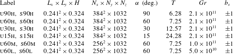
Geometry and parameters for the DNS runs.
 $L_{i}$
and
 $N_{i}$
denote the domain size and the number of collocation nodes in the three coordinate directions, respectively,
 $T$
denotes the characteristic oscillation period characterizing the buoyancy and velocity fields (see § 3.4),
 $\mathit{Gr}\equiv \hat{b}_{s}^{4}\,\hat{\unicode[STIX]{x1D708}}^{-2}\,\hat{N}^{-6}$
where
 $b_{s}$
is the imposed (normalized) surface buoyancy. Simulation labels indicate whether a specific run is in buoyantly [u]nstable or [s]table regime (
 $b_{s}=+1$
and
 $b_{s}=-1$
respectively), the surface sloping angles
 $\unicode[STIX]{x1D6FC}$
, and which among the three considered Grashof numbers ([h]igh, [m]edium and [l]ow) is used; for instance u30h denotes an anabatic flows regime with
 $\unicode[STIX]{x1D6FC}=30^{\circ }$
at the highest among the considered Grashof numbers.
3 Simulations
Equations (2.9)–(2.11) are integrated across a range of sloping angles,
 $\unicode[STIX]{x1D6FC}$
and
 $Gr$
numbers, considering both anabatic (upslope) and katabatic (downslope) flow regimes, as summarized in table 1. Given the computational cost of DNS, variations in
 $Gr$
are limited to the
 $\unicode[STIX]{x1D6FC}=60^{\circ }$
case.
Note that
 $(b,\unicode[STIX]{x1D6FC})\rightarrow (-b,\unicode[STIX]{x1D6FC}+\unicode[STIX]{x03C0})$
is a symmetry transformation for the system (2.9)–(2.11), and therefore cases u90h and s90h are equivalent up to a change in the sign of
 $u_{i}$
. Because of this symmetry, a heated wall at
 $\unicode[STIX]{x1D6FC}=15^{\circ }$
is equivalent to a cooled wall at
 $\unicode[STIX]{x1D6FC}=15^{\circ }+180^{\circ }$
.
The DNS algorithm is a modification of the code previously used to study land–atmosphere interaction processes (Albertson & Parlange Reference Albertson and Parlange1999a
,Reference Albertson and Parlange
b
; Kumar et al.
Reference Kumar, Kleissl, Meneveau and Parlange2006; Bou-Zeid et al.
Reference Bou-Zeid, Overney, Rogers and Parlange2009; Calaf, Meneveau & Meyers Reference Calaf, Meneveau and Meyers2010; Calaf, Parlange & Meneveau Reference Calaf, Parlange and Meneveau2011; Giometto et al.
Reference Giometto, Christen, Meneveau, Fang, Krafczyk and Parlange2016; Sharma et al.
Reference Sharma, Calaf, Lehning and Parlange2016; Sharma, Parlange & Calaf Reference Sharma, Parlange and Calaf2017), to develop and test linear and nonlinear LES subgrid-scale models (Porté-Agel, Meneveau & Parlange Reference Porté-Agel, Meneveau and Parlange2000; Higgins, Parlange & Meneveau Reference Higgins, Parlange and Meneveau2003; Bou-Zeid, Meneveau & Parlange Reference Bou-Zeid, Meneveau and Parlange2005; Lu & Porté-Agel Reference Lu and Porté-Agel2010; Abkar, Bae & Moin Reference Abkar, Bae and Moin2016), to design surface-flux parameterizations (Hultmark, Calaf & Parlange Reference Hultmark, Calaf and Parlange2013) and to model scalar transport processes (Chamecki, Meneveau & Parlange Reference Chamecki, Meneveau and Parlange2009). Equations are solved in rotational form to ensure conservation of mass and kinetic energy (Orszag & Pao Reference Orszag and Pao1975). A pseudospectral collocation approach (Orszag Reference Orszag1969, Reference Orszag1970) based on truncated Fourier expansions is used in the
 $x,y$
coordinate directions whereas a second-order accurate centred finite differences scheme is adopted in the slope-normal direction, requiring a staggered grid approach for the
 $u,v,p,b$
state variables (these are stored at
 $(i+1/2)\unicode[STIX]{x1D6E5}_{Z}$
, where
 $i$
denotes a given layer of collocation nodes in the slope-normal direction). Time integration is performed adopting a fully explicit second-order accurate Adams–Bashforth scheme. A fractional step method (Chorin Reference Chorin1968; Temam Reference Temam1968) is adopted to compute the pressure field by solving an additional Poisson equation, which is derived enforcing mass continuity for the incompressible fluid
 $(\unicode[STIX]{x2202}u_{i}/\unicode[STIX]{x2202}x_{i}=0)$
. Further, all nonlinear terms are fully de-aliased adopting a
 $3/2$
rule so as to avoid artificial pile up of energy at the high wavenumber range (Kravchenko & Moin Reference Kravchenko and Moin1997; Canuto et al.
Reference Canuto, Hussaini, Quarteroni and Zang2006).
Equations are integrated over a regular domain
 $[0,L_{x}]\times [0,L_{y}]\times [0,H]$
, with boundary conditions
 $u_{i}(x,y,0)=u_{i}(x,y,H)=b(x,y,H)=0$
and
 $b(x,y,0)=\hat{b}_{s}/\hat{B}=\pm 1$
.
A sponge layer (Israeli & Orszag Reference Israeli and Orszag1981) is applied to the top
 $20\,\%$
of the computational domain so as to damp spurious internal wave reflections. The thickness of the sponge layer has been chosen based on a sensitivity analysis performed on the s15h case, which showed that a minimum of 15 % thickness is required to avoid non-negligible TKE at the top of the computational domain.
To guide the choice of the grid stencil an estimate of
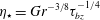 $\unicode[STIX]{x1D702}_{\star }=\mathit{Gr}^{-3/8}\unicode[STIX]{x1D70F}_{bz}^{-1/4}$
for the
 $\unicode[STIX]{x1D6FC}=90^{\circ }$
case was first evaluated from the Prandtl laminar flow analytic solution, where
 $\unicode[STIX]{x1D702}_{\star }$
is an equivalent of the Kolmogorov scale (FS2009) in the chosen normalized units, and where
 $\unicode[STIX]{x1D70F}_{bz}$
denotes the normalized kinematic surface buoyancy flux. Subsequently the grid stencils were set to
 $\unicode[STIX]{x1D6E5}_{x}=\unicode[STIX]{x1D6E5}_{y}=2\unicode[STIX]{x1D6E5}_{z}=2\unicode[STIX]{x1D702}_{\star }$
. The resolvability condition
 $\unicode[STIX]{x1D6E5}<2\unicode[STIX]{x1D702}$
(Pope Reference Pope2000) has been checked a posteriori (not shown) for all the considered cases, where
 $\unicode[STIX]{x1D702}=\mathit{Gr}^{-3/8}\unicode[STIX]{x1D716}^{-1/4}$
is the Kolmogorov length scale in normalized units. The vertical grid stencil satisfies such a criterion in all cases, whereas the horizontal grid stencil is often off by a factor of two, hence the need to verify the quality of proposed results. To do so, a higher resolution DNS katabatic run was performed at a sloping angle
 $\unicode[STIX]{x1D6FC}=90^{\circ }$
, halving the horizontal grid stencil (i.e. doubling the resolution in the horizontal directions). Note that the Kolmogorov scale is usually larger in stable cases than in the neutral ones, hence slope flows over vertical walls (
 $\unicode[STIX]{x1D6FC}=90^{\circ }$
) have the most stringent resolution requirements. First- and second-order statistics are found to be in good agreement with those presented herein, supporting the working conjecture that the current resolution is sufficient to represent most of the dissipative scales. The resulting domain size (see table 1) allows the representation of coherent structures populating the DBL and TBL at all the considered sloping angles (a domain-size convergence study was performed for the anabatic case at
 $\unicode[STIX]{x1D6FC}=15^{\circ }$
to support such assertion, and variations of statistics were found to be negligible).
Simulations are run for a minimum of
 $6T$
, where
 $T=2\unicode[STIX]{x03C0}\sin ^{-1}\unicode[STIX]{x1D6FC}$
is the characteristic (normalized) period of internal waves that arise in the system due to the imposed stable background stratification. Statistics are computed over the last
 $5T$
for the cases
 $\unicode[STIX]{x1D6FC}=90^{\circ },\unicode[STIX]{x1D6FC}=60^{\circ }$
, and over the last
 $3T$
for the cases
 $\unicode[STIX]{x1D6FC}=30^{\circ },\unicode[STIX]{x1D6FC}=15^{\circ }$
(previous time steps are disregarded to allow turbulence to fully develop). All simulations are performed using
 $Pr=1$
, in line with previous studies of slope flows (FS09). Throughout,
 $\langle \cdot \rangle$
denotes averaging in time and along spatial coordinates of statistical homogeneity
 $(x,y)$
and fluctuations with respect to time and space averages
 $(\langle \cdot \rangle )$
are expressed as
 $(\cdot )^{\prime }$
.
4 Results and discussion
Throughout this section, unless otherwise stated, all results and comments regard cases characterized by
 $\mathit{Gr}=2\times 10^{11}$
. Variations of the solution with respect to
 $Gr$
are described and commented in appendix A.
4.1 Time evolution and structure of the flow
The time evolution of the slope-normal integrated, space-averaged (
 $x,y$
directions), normalized streamwise velocity
 $\langle u\rangle$
and buoyancy
 $\langle b\rangle$
is displayed in figure 2. The system exhibits the classical quasi-periodic, low-frequency, oscillatory behaviour (surges), superimposed to a base flow, as observed in FS09 and in experiments (e.g. Doran & Horst Reference Doran and Horst1981; Monti et al.
Reference Monti, Fernando, Princevac, Chan, Kowalewski and Pardyjak2002; Princevac, Hunt & Fernando Reference Princevac, Hunt and Fernando2008). It can be shown (McNider Reference McNider1982) that the slope-normal integrated
 $\langle u\rangle ,\,\langle b\rangle$
variables resemble a system of coupled oscillators, which in the case of laminar flow are characterized by a period
 $\hat{T}\approx 2\unicode[STIX]{x03C0}(\hat{N}\sin \unicode[STIX]{x1D6FC})^{-1}$
(normalized period is
 $T\approx 2\unicode[STIX]{x03C0}/\sin \unicode[STIX]{x1D6FC}$
). The oscillation periods from DNS are very close to those of corresponding laminar solutions, which for typical atmospheric values
 $\hat{N}=10^{-2}\,(\text{Hz})$
,
 $\unicode[STIX]{x1D6FC}=15^{\circ },\,30^{\circ }$
and
 $60^{\circ }$
, are
 $40,\,20$
and 10 min. A recent study (Fedorovich & Shapiro Reference Fedorovich and Shapiro2017) has shown how damping of integral oscillations by surface stress in laminar Prandtl flows decays very rapidly and independently from the flow forcing mechanism. Such fast reduction in the damping factor was also observed in the turbulent slope flows simulated in FS09. Current results further support such findings, i.e. observed integral oscillations are characterized by a progressively weaker decay rate as time advances.
Time evolution of slope-normal integrated
 $\langle u\rangle$
(solid lines) and
 $\langle b\rangle$
(dashed lines) fields for simulations s90h, s60h, s30h and s15h (katabatic flow regime). The total time integration period is shown for each run.

Dynamic (black lines) and energy (red lines) identities (4.1) and (4.2) for the considered simulations. Profiles have been shifted on the
 $y$
axis to allow for proper visualization. From top to bottom, profiles correspond to u15h, u30h, u60h, u90h and s15h, s30h, s60h, s90h, respectively. We here denote
 $\langle \unicode[STIX]{x1D70F}_{xz}^{tot}\rangle =\mathit{Gr}^{-1/2}(\text{d}\langle u\rangle /\text{d}z)-\langle u^{\prime }w^{\prime }\rangle$
and
 $\langle \unicode[STIX]{x1D70F}_{bz}^{tot}\rangle =\mathit{Gr}^{-1/2}Pr^{-1}(\text{d}\langle b\rangle /\text{d}z)-\langle b^{\prime }w^{\prime }\rangle$
(sum of molecular and turbulent kinematic fluxes of streamwise momentum and buoyancy in the slope-normal direction).

Averaging equations (2.9)–(2.11) in time and over directions of statistical homogeneity
 $(x,y)$
results in
 $$\begin{eqnarray}\displaystyle & \displaystyle \langle b\rangle \sin (\unicode[STIX]{x1D6FC})=\frac{\text{d}\langle \unicode[STIX]{x1D70F}_{xz}^{tot}\rangle }{\text{d}z}, & \displaystyle\end{eqnarray}$$
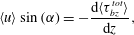 $$\begin{eqnarray}\displaystyle & \displaystyle \langle u\rangle \sin (\unicode[STIX]{x1D6FC})=-\frac{\text{d}\langle \unicode[STIX]{x1D70F}_{bz}^{tot}\rangle }{\text{d}z}, & \displaystyle\end{eqnarray}$$
where
 $\langle \unicode[STIX]{x1D70F}_{xz}^{tot}\rangle =\mathit{Gr}^{-1/2}(\text{d}\langle u\rangle /\text{d}z)-\langle u^{\prime }w^{\prime }\rangle$
and
 $\langle \unicode[STIX]{x1D70F}_{bz}^{tot}\rangle =\mathit{Gr}^{-1/2}Pr^{-1}(\text{d}\langle b\rangle /\text{d}z)-\langle b^{\prime }w^{\prime }\rangle$
are the normalized total (molecular
 $+$
turbulent) slope-normal kinematic momentum and buoyancy fluxes. Equations (4.1) and (4.2) can be used to test the ‘quality’ of computed statistics (steady state is guaranteed only if the two identities hold). Numerical results are displayed in figure 3, and certify that averaging over
 $3T$
, after a transient of at least
 $3T$
is sufficient to satisfy both equations (4.1) and (4.2).
Pseudocolour plot of instantaneous katabatic flow streamwise velocity
 $u$
(a,b) and buoyancy
 $b$
(c,d), on the plane
 $y=L_{y}/2$
for simulations s60h (a,c) and s15h (b,d). The
 $z$
-axis denotes the slope-normal coordinate direction, whereas the
 $x$
-axis denotes the along-slope direction. The displayed
 $u(x,z)$
and
 $b(x,z)$
fields correspond to the crest of the last simulated oscillation for both runs. For detailed viewing, only the near-surface region of the total domain is shown.

Pseudocolour plot of instantaneous anabatic flow streamwise velocity
 $u$
(a,b) and buoyancy
 $b$
(c,d), on the plane
 $y=L_{y}/2$
for simulations u60h (a,c) and u15h (b,d). The displayed
 $u(x,z)$
and
 $b(x,z)$
fields correspond to the crest of the last simulated oscillation for both runs. For detailed viewing, only the near-surface region of the total domain is shown.

Figures 4 and 5 display a pseudocolour plot of instantaneous streamwise normalized velocity field
 $(u)$
and normalized buoyancy field
 $(b)$
for simulations s60h, s15h and u60h, u15h, respectively. The TBL appears shallower than the DBL, as previously noted in FS09. A reversed flow characterizes the above-jet regions, resulting from the interaction between the flow and the background stably stratified environment, in qualitative agreement with the predictions of the Prandtl model (Prandtl Reference Prandtl1942). Progressive dissimilarity in DBL and TBL boundary layer thickness arises as the sloping angle decreases from the reference
 $\unicode[STIX]{x1D6FC}=90^{\circ }$
vertical wall set-up (recall that at
 $\unicode[STIX]{x1D6FC}=90^{\circ }$
the two flow regimes are equal up to a sign in
 $u_{i}$
). As
 $\unicode[STIX]{x1D6FC}$
decreases, the LLJ regions in the anabatic flow solution experience a significant thickening induced by the convective type regime characterizing the flow at small sloping angles. Katabatic flows are instead characterized by a strong static stability at small sloping angles (see figure 4), which damps positive slope-normal velocity fluctuations, thus maintaining the LLJ relatively close to the wall and reducing the overall mixing of momentum and buoyancy in the near-wall regions. In addition, the strong stability induced by the imposed surface buoyancy in the katabatic flow regime at small
 $\unicode[STIX]{x1D6FC}$
results in partial laminarization of the LLJ.
4.2 Mean flow
Mean profiles of kinematic momentum
 $\langle u\rangle$
and buoyancy
 $\langle b\rangle$
are displayed in figure 6. Computed quantities qualitatively resemble those from the classic constant-K Prandtl analytic solution (Prandtl Reference Prandtl1942). The most significant features are a peak velocity
 $(u_{j})$
, the nose of the LLJ (occurring at
 $z_{j}$
), and a return flow region capping both the DBL and TBL. As previously observed in FS09, such features are sensitive to the sloping angle
 $(\unicode[STIX]{x1D6FC})$
, and as
 $\unicode[STIX]{x1D6FC}$
decreases from the vertical wall set-up (
 $\unicode[STIX]{x1D6FC}=90^{\circ }$
), the anabatic and katabatic flow solutions progressively depart from each other.
Comparison of streamwise mean velocity
 $\langle u\rangle$
(a) and
 $\langle u^{+}\rangle$
(c) and of mean buoyancy
 $\langle b\rangle$
(b) and
 $\langle b^{+}\rangle$
(d) for anabatic (dashed lines) and katabatic (solid lines) flows. Symbols:
 $\unicode[STIX]{x1D6FC}=90^{\circ }$
, black lines;
 $\unicode[STIX]{x1D6FC}=60^{\circ }$
, blue lines;
 $\unicode[STIX]{x1D6FC}=30^{\circ }$
, green lines;
 $\unicode[STIX]{x1D6FC}=15^{\circ }$
, red lines. All cases are characterized by
 $\mathit{Gr}=2.1\times 10^{11}$
. The
 $z$
-axis denotes the slope-normal coordinate direction.

The constant-K Prandtl solution provides a useful framework for the interpretation of results, and is thus here briefly summarized. Based on the proposed normalization (see Sect. 2.1), the Prandtl one-dimensional solution for imposed constant surface buoyancy reads (FS09)
 $$\begin{eqnarray}\displaystyle & \displaystyle u=-b_{s}Pr^{-1/2}\sin (\unicode[STIX]{x1D70E}z)\exp (-\unicode[STIX]{x1D70E}z),\quad z\in [0,\infty ), & \displaystyle\end{eqnarray}$$
 $$\begin{eqnarray}\displaystyle & \displaystyle b=b_{s}\cos (\unicode[STIX]{x1D70E}z)\exp (-\unicode[STIX]{x1D70E}z),\quad z\in [0,\infty ), & \displaystyle\end{eqnarray}$$
where
 $\unicode[STIX]{x1D70E}=(\mathit{Gr}\,Pr^{-1})^{1/4}\sin (\unicode[STIX]{x1D6FC})^{1/2}$
and
 $b_{s}=\pm 1$
. Note that (4.3) and (4.4) correspond to a laminar flow solution of the time and space averaged (2.9)–(2.11). It predicts a velocity maximum
 $u_{j}=\pm 1/\sqrt{2}\exp (-\unicode[STIX]{x03C0}/4)$
that is independent of the sloping angle
 $(\unicode[STIX]{x1D6FC})$
, whereas the characteristic length scale of the flow
 $L\propto \sin (\unicode[STIX]{x1D6FC})^{-1/2}$
whereby
 $z_{j}\propto \sin (\unicode[STIX]{x1D6FC})^{-1/2}$
(Grisogono & Axelsen Reference Grisogono and Axelsen2012; Grisogono et al.
Reference Grisogono, Jurlina, Večenaj and Güttler2014).
The location of the LLJ for the katabatic flow DNS solution is in good agreement with prediction from the Prandtl laminar flow solution, i.e.
 $$\begin{eqnarray}z_{j}\approx \frac{\unicode[STIX]{x03C0}}{4\unicode[STIX]{x1D70E}}.\end{eqnarray}$$
Conversely,
 $u_{j}$
is significantly smaller (a reduction from
 ${\approx}30\,\%$
to
 ${\approx}50\,\%$
depending on the slope angle) when compared to the laminar solution, mainly due to additional diffusion of momentum caused by turbulent motions at
 $z_{j}$
(as shown in § 4.5). In addition,
 $u_{j}$
is not independent of
 $\unicode[STIX]{x1D6FC}$
as in the Prandtl model, but is characterized by a modest increase as
 $\unicode[STIX]{x1D6FC}$
decreases. This behaviour can be explained by considering that as the sloping angle decreases, the stable stratification induced by the imposed surface buoyancy damps turbulent motions in the LLJ region, thus reducing turbulent mixing of momentum and resulting in a higher peak velocity
 $u_{j}$
.
The anabatic flow solution is more sensitive to variations in the sloping angle, when compared to its katabatic counterpart. As
 $\unicode[STIX]{x1D6FC}$
is reduced, a simultaneous increase in the height of the LLJ and a reduction in its peak speed are observed. Variations are significant when compared to those characterizing the katabatic solution and the laminar case. This pattern is related to the strengthening of the slope-normal component of the buoyancy force as
 $\unicode[STIX]{x1D6FC}$
decreases (
 $b\unicode[STIX]{x1D6FF}_{i3}\cos \unicode[STIX]{x1D6FC}$
in (2.9)). This results in an unstable near-wall stratification, which enhances the slope-normal flux of momentum, and leads to progressively more mixed profiles of velocity and buoyancy in the LLJ regions, in agreement with the findings of FS09.
Figure 6 also features mean velocity and buoyancy profiles scaled with inner units, i.e.
 $z^{+}=\hat{z}\hat{u} _{\star }/\hat{\unicode[STIX]{x1D708}},\,u^{+}=\hat{u} /\hat{u} _{\star },\,b^{+}=\hat{b}/\hat{b}_{\star }$
(where
 $\hat{u} _{\star }\equiv \sqrt{\langle \unicode[STIX]{x1D70F}_{xz}^{tot}\rangle |_{z=0}}$
and
 $\hat{b}_{\star }\equiv (\langle \unicode[STIX]{x1D70F}_{bz}^{tot}\rangle |_{z=0})/u_{\star }$
, with
 $\unicode[STIX]{x1D70F}_{xz}^{tot}$
and
 $\unicode[STIX]{x1D70F}_{bz}^{tot}$
being the total kinematic momentum and buoyancy fluxes). The nose of the LLJ is located at
 $z^{+}\approx 25$
in katabatic flows, separating the viscosity dominated wall regions from the turbulent outer layers. Anabatic flow solutions are characterized by a progressively more mixed LLJ as the sloping angle decreases, with peak speed at
 $z^{+}\approx 100$
for
 $\unicode[STIX]{x1D6FC}=15^{\circ }$
, again highlighting a broadening of the DBL as the slope is reduced.
Another notable difference between the katabatic and the anabatic flow solutions is the sensitivity of the DBL and TBL thickness to
 $\unicode[STIX]{x1D6FC}$
. The DBL and TBL thickness (
 $\unicode[STIX]{x1D6FF}_{d}$
and
 $\unicode[STIX]{x1D6FF}_{t}$
respectively), which can be identified as the first and second zero crossing of
 $\langle b\rangle$
and
 $\langle u\rangle$
respectively are insensitive to
 $\unicode[STIX]{x1D6FC}$
for the katabatic flow regime, whereas they vary by a factor of three across the considered
 $\unicode[STIX]{x1D6FC}$
-range for the anabatic flow solution. In line with this finding, the slope-normal integrated horizontal momentum flux
 $(I_{u})$
in the anabatic flow regime is also strongly sensitive to variations in
 $\unicode[STIX]{x1D6FC}$
, whereas it is insensitive in the katabatic cases.
 $\unicode[STIX]{x1D6FC}$
dependence of the surface buoyancy flux
 $B_{w}$
for katabatic (a) and anabatic (b) flow cases. Simulations correspond to cases s90h, s60h, s30h, s15h and u90h, u60h, u30h, u15h for the katabatic and anabatic regimes, respectively. Predictions from the Prandtl laminar solution are included for comparison (black lines).

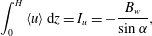
Such behaviour can be understood by integrating (4.2),
 $$\begin{eqnarray}\int _{0}^{H}\langle u\rangle \,\text{d}z=I_{u}=-\frac{B_{w}}{\sin \unicode[STIX]{x1D6FC}},\end{eqnarray}$$
where
 $B_{w}$
is the surface buoyancy flux. From (4.6) is apparent how larger
 $B_{w}$
and shallower slopes are characterized by larger
 $I_{u}$
. Variations of the surface buoyancy flux as a function of
 $\unicode[STIX]{x1D6FC}$
for the considered anabatic and katabatic cases are displayed in figure 7. As apparent, the anabatic flow solution is characterized by modest variations in
 $B_{w}$
across the considered
 $\unicode[STIX]{x1D6FC}$
range, when compared against the katabatic flow cases. The latter experience a significant decrease in the surface buoyancy flux as the sloping angle decreases from
 $90^{\circ }$
to
 $15^{\circ }$
, slowly approaching the surface flux predicted by the laminar flow solution (at
 $\unicode[STIX]{x1D6FC}=15^{\circ }$
the difference between the DNS surface flux and the laminar solution surface flux is only
 $20\,\%$
the magnitude of the DNS surface flux itself). Such a behaviour is closely related to the strengthening of the near-surface inversion layer, which damps turbulent motions and leads to an apparent laminarization of the flow. In contrast, anabatic flows depart from the laminar solution as
 $\unicode[STIX]{x1D6FC}$
decreases, due to the unstable stratification and likely onset of convective motions. Based on results shown in figure 7 one could introduce the equally crude approximations
 $$\begin{eqnarray}\displaystyle & \displaystyle B_{w}(\unicode[STIX]{x1D6FC})/B_{w}^{\unicode[STIX]{x1D6FC}=90^{\circ }}\approx 1\quad \text{for anabatic flows}, & \displaystyle\end{eqnarray}$$
 $$\begin{eqnarray}\displaystyle & \displaystyle B_{w}(\unicode[STIX]{x1D6FC})/B_{w}^{\unicode[STIX]{x1D6FC}=90^{\circ }}\approx \sin \unicode[STIX]{x1D6FC}\quad \text{for katabatic flows}, & \displaystyle\end{eqnarray}$$
which justifies the observed variations in the vertically integrated horizontal momentum flux in the anabatic and katabatic flow regimes based on (4.6).
Note that since
 $I_{u}={\mathcal{U}}{\mathcal{L}}$
, where
 ${\mathcal{U}}$
and
 ${\mathcal{L}}$
are the characteristic (normalized) velocity and length scale of the flow, and given that
 ${\mathcal{U}}\approx const.$
for both anabatic and katabatic flows, from (4.7) and (4.8) follows that
 ${\mathcal{L}}\propto 1/\sin \unicode[STIX]{x1D6FC}$
for anabatic flows, and
 ${\mathcal{L}}\approx const.$
for katabatic flows. Such information can be of use for scaling purposes.
Given the strong
 $\unicode[STIX]{x1D6FC}$
dependence of
 $B_{w}$
in the katabatic flow solution, profiles are expected vary significantly – when compared to those proposed herein – if a constant
 $B_{w}$
is used to drive the flow. Conversely,
 $B_{w}$
in the anabatic flow solution is weakly dependent on
 $\unicode[STIX]{x1D6FC}$
, and profiles are therefore expected to be poorly sensitive on the specific flow driving mechanisms (i.e. constant surface buoyancy or constant surface buoyancy flux). Because of this, the proposed anabatic flow solutions share strong similarities with those reported in the FS09 study, especially when considering the
 $\unicode[STIX]{x1D6FC}$
dependence of
 $z_{j},u_{j}$
and
 $\unicode[STIX]{x1D6FF}_{d},\unicode[STIX]{x1D6FF}_{t}$
, whereas the katabatic flow solutions differ significantly.
When a constant surface buoyancy flux is applied, the laminar flow solution is characterized by
 $z_{j}=\unicode[STIX]{x03C0}/(4\unicode[STIX]{x1D70E})$
and
 $u_{j}\propto (\sin (\unicode[STIX]{x1D6FC}))^{-1/2}$
(Grisogono & Axelsen Reference Grisogono and Axelsen2012; Grisogono et al.
Reference Grisogono, Jurlina, Večenaj and Güttler2014). Hence,
 $u_{j}$
increases as the sloping angle decreases and is not
 $\unicode[STIX]{x1D6FC}$
independent as predicted by (4.3) and (4.4).
Similar variations in
 $z_{j}$
and a stronger
 $\unicode[STIX]{x1D6FC}$
dependency of
 $u_{j}$
and
 $\unicode[STIX]{x1D6FF}_{d},\unicode[STIX]{x1D6FF}_{t}$
have been reported in FS09 for the katabatic flow solution when compared to current DNS results, qualitatively resembling predictions of the analytic laminar flow solution.
Note that when the flow is forced through a constant surface buoyancy flux, as in the FS09 study, anabatic and katabatic flow solutions are constraint to share the same slope-normal integrated horizontal momentum flux
 $I_{u}^{\unicode[STIX]{x1D6FC}}/I_{u}^{\unicode[STIX]{x1D6FC}=90^{\circ }}=1/\sin \unicode[STIX]{x1D6FC}$
, hence the stronger variability of
 $\unicode[STIX]{x1D6FF}_{d}$
and
 $\unicode[STIX]{x1D6FF}_{t}$
in the FS09 katabatic flow solution, when compared to the current DNS results.
4.3 TKE and buoyancy variance
Slope-normal variations of TKE and of buoyancy variance
 $\langle b^{\prime }b^{\prime }\rangle$
are featured in figure 8. The buoyancy variance may also be interpreted as a form of turbulent potential energy. The stronger surface stable stratification that characterizes katabatic flows as the sloping angle decreases results in a weakening of TKE in the inner flow regions (below the LLJ), whereas the observed increase of TKE in the outer flow region as
 $\unicode[STIX]{x1D6FC}$
decreases is likely related to the broadening of the flow length scales, which despite being modest for the katabatic flow solution, have an apparent effect on TKE. TKE profiles from the anabatic flow solution are again more sensitive to
 $\unicode[STIX]{x1D6FC}$
when compared to their katabatic counterparts. In the anabatic flow cases, the peak TKE location increases as
 $\unicode[STIX]{x1D6FC}$
decreases, but its magnitude shows non-monotonic behaviour, thus suggesting a more complex dependence on
 $\unicode[STIX]{x1D6FC}$
. Furthermore, the TKE in the neighbourhood of the LLJ is approximately constant throughout the considered flow regimes.
Comparison of turbulent kinetic energy
 $(1/2)\langle u_{i}^{\prime }u_{i}^{\prime }\rangle$
(a) and buoyancy variance
 $(\langle b^{\prime }b^{\prime }\rangle )$
(b) for the katabatic (solid lines) and the anabatic flow (dashed lines) regimes at
 $\unicode[STIX]{x1D6FC}=90^{\circ }$
(black),
 $\unicode[STIX]{x1D6FC}=60^{\circ }$
(blue),
 $\unicode[STIX]{x1D6FC}=30^{\circ }$
(green), and
 $\unicode[STIX]{x1D6FC}=15^{\circ }$
(red). Simulations correspond to the highest
 $\mathit{Gr}=2.1\times 10^{11}$
cases. Recall that the
 $z$
-axis denotes the slope-normal coordinate direction.

Normal stress components
 $\langle u^{\prime }u^{\prime }\rangle$
(solid lines),
 $\langle v^{\prime }v^{\prime }\rangle$
(dashed lines) and
 $\langle w^{\prime }w^{\prime }\rangle$
(dot-dashed lines) for the katabatic (a) and the anabatic (b) flow regimes at
 $\unicode[STIX]{x1D6FC}=90^{\circ }$
(black),
 $\unicode[STIX]{x1D6FC}=60^{\circ }$
(blue),
 $\unicode[STIX]{x1D6FC}=30^{\circ }$
(green) and
 $\unicode[STIX]{x1D6FC}=15^{\circ }$
(red). Simulations correspond to the highest
 $\mathit{Gr}=2.1\times 10^{11}$
cases (simulations s90h, s60h, s30h, and s15h and u90h, u60h, u30h and u15h, respectively).

The buoyancy variance
 $\langle b^{\prime }b^{\prime }\rangle$
peaks in the near-wall regions for both flow regimes where strong buoyancy gradients occur, in agreement with findings from FS09. Variations in
 $\langle b^{\prime }b^{\prime }\rangle$
as a function of
 $\unicode[STIX]{x1D6FC}$
in the below-LLJ region are significant only for the katabatic flow regime, with peak value and its location increasing and decreasing as
 $\unicode[STIX]{x1D6FC}$
is reduced. The above-LLJ regions of the boundary layer are characterized by a rapid decay in
 $\langle b^{\prime }b^{\prime }\rangle$
, most evident for the katabatic flow regime. The anisotropic nature of turbulence in slope flows is apparent from figure 9, where normal stress components
 $\langle u^{\prime }u^{\prime }\rangle$
,
 $\langle v^{\prime }v^{\prime }\rangle$
and
 $\langle w^{\prime }w^{\prime }\rangle$
are compared. The boundary layer character of the system is apparent with the wall providing an effective damping of the
 $\langle w^{\prime }w^{\prime }\rangle$
central moment, in both anabatic and katabatic flow regimes. It is to be noted the strong sensitivity of
 $\langle w^{\prime }w^{\prime }\rangle$
with respect to
 $\unicode[STIX]{x1D6FC}$
for both wind regimes. This behaviour is related to the direct effect of stratification (background
 $+$
perturbation) on
 $\langle w^{\prime }w^{\prime }\rangle$
, given that buoyancy is effective at damping/exciting slope-normal velocity fluctuations
 $w^{\prime }$
. Because of this, as
 $\unicode[STIX]{x1D6FC}$
decreases, the turbulence characterizing katabatic flows becomes more anisotropic (the strong, effective, stable stratification damps
 $\langle w^{\prime }w^{\prime }\rangle$
) in contrast to its anabatic counterpart, where the positive surface buoyancy leads to more isotropic turbulent motions. The observed trend here supports the recently proposed scaling of Shapiro & Fedorovich (Reference Shapiro and Fedorovich2014) based on the assumption of large-scale separation between slope-normal and slope-parallel motions populating katabatic flows, which might indeed hold at small sloping angles.
Total (solid lines) and turbulent (dashed lines) momentum flux for the katabatic (a) and the anabatic (b) flow regimes, and total (solid lines) and turbulent (dashed lines) buoyancy slope-normal flux for the katabatic (c) and the anabatic (d) flow regimes. All cases are characterized by
 $\mathit{Gr}=2.1\times 10^{11}$
.
 $\langle \unicode[STIX]{x1D70F}_{xz}^{tot}\rangle$
denotes the total slope-normal flux of momentum, whereas
 $\langle \unicode[STIX]{x1D70F}_{bz}^{tot}\rangle$
denotes the total slope-normal buoyancy flux. The height of the LLJ (
 $z_{j}$
) is displayed (horizontal lines) for the different cases to provide a reference.

4.4 Momentum and buoyancy fluxes
Turbulent and total (turbulent
 $+$
molecular) vertical buoyancy and momentum fluxes are displayed in figure 10 for each of the considered runs. Turbulent buoyancy fluxes obey Fick’s law of diffusion, whereas momentum fluxes consistently feature a thin layer just below the LLJ where counter gradient fluxes are observed. This feature is related to the extrema of the mean
 $\langle u\rangle$
-profiles not being co-located with the zero crossing of the turbulent momentum fluxes. At the LLJ location for instance, a positive (negative) total slope-normal momentum flux for the katabatic (anabatic) flow regime are observed. Note that counter gradient fluxes have been previously reported in experimental studies (Smeets et al.
Reference Smeets, Duynkerke and Vugts2000; Oldroyd et al.
Reference Oldroyd, Pardyjak, Higgins and Parlange2016a
). The peak magnitude of both
 $\langle \unicode[STIX]{x1D70F}_{xz}^{tot}\rangle$
and
 $\langle \unicode[STIX]{x1D70F}_{bz}^{tot}\rangle$
in the above-LLJ regions is dependent on
 $\unicode[STIX]{x1D6FC}$
for both flow regimes (it decreases as
 $\unicode[STIX]{x1D6FC}$
decreases). In addition, katabatic flow solutions are characterized by a modest upward shift of flux extrema as the sloping angle decreases, whereas the upward shift is more significant for the anabatic flow cases. Such trends are directly related to the combined effects of
 $\unicode[STIX]{x1D6FC}$
on the scales of the flow (recall that the analytic Prandtl solution predicts
 $L\propto (\sin (\unicode[STIX]{x1D6FC}))^{-1/2}$
) and of the surface induced stratification in katabatic and anabatic flows, whose strength increases as
 $\unicode[STIX]{x1D6FC}$
decreases, progressively damping (for the katabatic cases) or enhancing (for the anabatic cases) turbulent fluctuations. In the FS09 study, the peak magnitude of
 $\langle \unicode[STIX]{x1D70F}_{xz}^{tot}\rangle$
and
 $\langle \unicode[STIX]{x1D70F}_{bz}^{tot}\rangle$
in the katabatic flow regime was found to be approximately constant and independent of
 $\unicode[STIX]{x1D6FC}$
. Conversely, it was sensitive to
 $\unicode[STIX]{x1D6FC}$
in the anabatic flow cases, in apparent contrast with current findings. Such a mismatch is related to the different surface forcing approach that characterizes the current and the FS90 study (in FS90 a constant surface buoyancy flux is applied to drive the flow).
Total (solid lines) and turbulent (dashed lines) momentum flux for the katabatic (a) and the anabatic (b) flow regimes in inner units. All cases are characterized by
 $\mathit{Gr}=2.1\times 10^{11}$
.
 $\langle \unicode[STIX]{x1D70F}_{xz}^{tot}\rangle$
denotes the total slope-normal flux of momentum. The height of the LLJ (
 $z_{j}$
) is displayed (horizontal lines) for the different cases to provide a reference.

Figure 11 features the total and the turbulent momentum fluxes for the considered katabatic and anabatic flow regimes in inner units. For katabatic flows the viscous contribution to the total flux is dominant in the below-LLJ regions, and drops to less than
 $10\,\%$
as
 $z^{+}>50$
for the
 $\unicode[STIX]{x1D6FC}=90^{\circ }$
case. As the sloping angle decreases the viscous contribution in the above-LLJ region increases, due to the strengthening of the stable stratification resulting from the imposed surface buoyancy, and amounts to approximately
 $35\,\%$
the total at
 $z^{+}=50$
for the shallower of the considered slopes
 $(\unicode[STIX]{x1D6FC}=15^{\circ })$
. In contrast, anabatic flows are characterized by a decrease of viscous contributions to the total momentum flux as the sloping angle decreases throughout the boundary layer, with viscous effects remaining dominant up to
 $z^{+}\approx 12$
, where viscous and turbulent fluxes are roughly of the same magnitude, and becoming negligible
 $({<}10\,\%)$
as
 $z^{+}>50$
. From figure 11 is also apparent how the surface contribution in terms of total stress is larger than the peak stress in the above-LLJ region for katabatic flows, whereas for anabatic flows as the sloping angle decreases the surface stress becomes progressively smaller when compared to the outer stress peak.
 $\unicode[STIX]{x1D6FC}$
dependence of the kinematic surface average stress
 $\unicode[STIX]{x1D70F}_{w}$
for katabatic (a) and anabatic (b) flow cases. Simulations correspond to cases s90h, s60h, s30h, s15h and u90h, u60h, u30h, u15h for the katabatic and anabatic regimes, respectively. Predictions from the Prandtl laminar solution are included for comparison (black lines).

Turbulent fluctuations contribute to the overall buoyancy flux in the below-LLJ region of katabatic flows, whereas they provide a negligible contribution to the overall momentum flux. This latter behaviour has direct effect on the overall surface stress, which is nearly equal to the laminar flow prediction for
 $\unicode[STIX]{x1D6FC}>90^{\circ }$
, as displayed in figure 12. Turbulent motion in the below-jet regions of katabatic flows are thus ‘inactive’ from a momentum transport perspective (in the Townsend (Reference Townsend1956) sense), but are relatively effective in vertically transporting buoyancy. To the contrary, turbulent fluctuations in the anabatic flow solution contribute to both the overall surface buoyancy and momentum fluxes that progressively depart from their Prandtl ‘laminar flow’ counterparts as
 $\unicode[STIX]{x1D6FC}$
is reduced. An interesting feature of the considered anabatic flow simulations is the magnitude of the time- and space-averaged surface total momentum flux (
 $\unicode[STIX]{x1D70F}_{w}$
), as displayed in figure 12.
 $\unicode[STIX]{x1D70F}_{w}$
is consistently smaller than its laminar flow prediction in the anabatic cases, and its magnitude decreases as the sloping angle is reduced. Note that such feature might be related to the relatively modest
 $Gr$
value characterizing the various runs.
4.5 The mean kinetic energy budget
The governing equation for the time- and space-averaged velocity
 $\langle u_{i}\rangle$
is readily derived by applying Reynolds decomposition to the instantaneous flow variables (e.g.
 $u_{i}=\langle u_{i}\rangle +u_{i}^{\prime }$
) and space
 $+$
time averaging (2.9). The budget equation for MKE is then obtained by multiplying the equation for
 $\langle u_{i}\rangle$
by
 $\langle u_{i}\rangle$
itself. Assuming horizontal homogeneity
 $(\unicode[STIX]{x2202}\langle \cdot \rangle /\unicode[STIX]{x2202}x=\unicode[STIX]{x2202}\langle \cdot \rangle /\unicode[STIX]{x2202}y=0)$
and no subsidence (
 $\langle w\rangle =0$
) it reads
 $$\begin{eqnarray}\displaystyle \frac{\unicode[STIX]{x2202}(\frac{1}{2}\langle u\rangle \langle u\rangle )}{\unicode[STIX]{x2202}t}=\langle u^{\prime }w^{\prime }\rangle \frac{\unicode[STIX]{x2202}\langle u\rangle }{\unicode[STIX]{x2202}z}-\langle u\rangle \langle b\rangle \sin (\unicode[STIX]{x1D6FC})-\frac{\unicode[STIX]{x2202}(\frac{1}{2}\langle u\rangle \langle u^{\prime }w^{\prime }\rangle )}{\unicode[STIX]{x2202}z}+\mathit{Gr}^{-1/2}\langle u\rangle \frac{\unicode[STIX]{x2202}^{2}\langle u\rangle }{\unicode[STIX]{x2202}z^{2}}, & & \displaystyle\end{eqnarray}$$
where the left-hand side of (4.9) is the storage term of MKE,
 ${\mathcal{P}}_{s}\equiv \langle u^{\prime }w^{\prime }\rangle (\unicode[STIX]{x2202}\langle u\rangle /\unicode[STIX]{x2202}z)$
denotes shear production/destruction of MKE,
 ${\mathcal{P}}_{b}\equiv -\langle u\rangle \langle b\rangle \sin (\unicode[STIX]{x1D6FC})$
denotes buoyancy production/destruction of MKE, transport of MKE by turbulent motions is
 ${\mathcal{T}}_{t}\equiv -\unicode[STIX]{x2202}(1/2\langle u\rangle \langle u^{\prime }w^{\prime }\rangle )/\unicode[STIX]{x2202}z$
and dissipation of MKE by viscous diffusion is
 ${\mathcal{E}}\equiv \mathit{Gr}^{-1/2}\langle u\rangle (\unicode[STIX]{x2202}^{2}\langle u\rangle /\unicode[STIX]{x2202}z^{2})$
. When time averaging over a sufficiently long time period then
 $\unicode[STIX]{x2202}\langle \cdot \rangle /\unicode[STIX]{x2202}t=0$
and the storage term can be neglected.
The normalized MKE budget terms for the considered anabatic and katabatic runs are displayed in figure 13. The choice of
 $\hat{b_{s}}^{2}\hat{N}^{-1}$
as a normalizing factor is not critical for the interpretation of the budget, since the relative magnitude of the terms is unchanged. As expected, the overall main source of MKE is from buoyancy production
 $({\mathcal{P}}_{b})$
, which peaks in the below-jet regions, and is characterized by a gradual decrease throughout the boundary layer. In the outer regions of the flow,
 ${\mathcal{P}}_{b}$
becomes a sink of MKE in both flow regimes starting from the zero crossing of
 $\langle b\rangle$
and up to the start of the return flow region. Here, energy is provided by turbulent transport
 $({\mathcal{T}}_{t})$
, which balances shear production
 $({\mathcal{P}}_{s})$
and buoyant production
 $({\mathcal{P}}_{b})$
(both
 ${\mathcal{P}}_{s}$
and
 ${\mathcal{P}}_{b}$
are a sink term of MKE in such layer). At the wall, buoyant production is overcome by dissipation for both upslope and downslope flows, and transport from turbulent motions is responsible to close the MKE budget.
 ${\mathcal{T}}_{t}$
acts as a sink of MKE in the highly energetic LLJ regions, displacing it toward the wall to balance the enhanced dissipation, and also into the outer layer of the flow.
Slope-normal structure of the MKE budget for the katabatic (a) and for the anabatic (b) flow regimes at
 $\unicode[STIX]{x1D6FC}=90^{\circ }$
(solid lines),
 $\unicode[STIX]{x1D6FC}=60^{\circ }$
(dashed lines),
 $\unicode[STIX]{x1D6FC}=30^{\circ }$
(dot-dashed lines) and
 $\unicode[STIX]{x1D6FC}=15^{\circ }$
(dotted lines). All cases are characterized by
 $\mathit{Gr}=2.1\times 10^{11}$
. The location of the LLJ is highlighted by horizontal lines for the various runs to provide a reference height (note that as
 $\unicode[STIX]{x1D6FC}$
decreases the LLJ height increases). All terms are normalized by
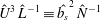 $\hat{U} ^{3}\,\hat{L}^{-1}\equiv \hat{b_{s}}^{2}\,\hat{N}^{-1}$
.

In both anabatic and katabatic flow regimes, shear production of MKE
 $({\mathcal{P}}_{s})$
acts as a sink of MKE in the above-jet regions, draining energy from the mean flow and transferring it to turbulence through the classical energy cascade process. Interestingly, for both regimes and all the considered sloping angles, the below-jet regions are characterized by
 ${\mathcal{P}}_{s}>0$
, highlighting a region of global energy backscatter, i.e. energy is transferred from the turbulent eddies to the mean flow. Forward scatter is known to be mainly caused by vortex stretching by the mean strain rate, whereas backscatter indicates vortex compression by the mean strain rate, which is not commonly observed in canonical wall-bounded flows.
4.6 The turbulent kinetic energy budget
Under the assumptions leading to (4.9), the budget equation for TKE is given as
 $$\begin{eqnarray}\displaystyle \frac{\unicode[STIX]{x2202}\langle \frac{1}{2}u_{i}^{\prime }u_{i}^{\prime }\rangle }{\unicode[STIX]{x2202}t} & = & \displaystyle -\langle u^{\prime }w^{\prime }\rangle \frac{\unicode[STIX]{x2202}\langle u\rangle }{\unicode[STIX]{x2202}z}+\langle b^{\prime }w^{\prime }\rangle \cos (\unicode[STIX]{x1D6FC})-\langle b^{\prime }u^{\prime }\rangle \sin (\unicode[STIX]{x1D6FC})-\frac{\unicode[STIX]{x2202}\langle \frac{1}{2}u_{i}^{\prime }u_{i}^{\prime }w^{\prime }\rangle }{\unicode[STIX]{x2202}z}\nonumber\\ \displaystyle & & \displaystyle -\,\frac{\unicode[STIX]{x2202}\langle \unicode[STIX]{x03C0}^{\prime }w^{\prime }\rangle }{\unicode[STIX]{x2202}z}+\mathit{Gr}^{-1/2}\frac{\unicode[STIX]{x2202}^{2}\langle \frac{1}{2}u_{i}^{\prime }u_{i}^{\prime }\rangle }{\unicode[STIX]{x2202}z^{2}}-\mathit{Gr}^{-1/2}\left<\frac{\unicode[STIX]{x2202}u_{i}^{\prime }}{\unicode[STIX]{x2202}x_{j}}\frac{\unicode[STIX]{x2202}u_{i}^{\prime }}{\unicode[STIX]{x2202}x_{j}}\right>,\end{eqnarray}$$
where
 $\unicode[STIX]{x2202}\langle (1/2)u_{i}^{\prime }u_{i}^{\prime }\rangle /\unicode[STIX]{x2202}t$
is the storage of TKE term, shear production of TKE is denoted as
 $P_{s}\equiv -\langle u^{\prime }w^{\prime }\rangle (\unicode[STIX]{x2202}\langle u\rangle /\unicode[STIX]{x2202}z)$
, buoyant production/destruction of TKE is composed of two terms, namely
 $P_{b,1}\equiv \langle b^{\prime }u^{\prime }\rangle \sin (\unicode[STIX]{x1D6FC})$
and
 $P_{b,3}\equiv \langle b^{\prime }w^{\prime }\rangle \cos (\unicode[STIX]{x1D6FC})$
, turbulent transport of TKE is
 $T_{t}\equiv -\unicode[STIX]{x2202}\langle (1/2)u_{i}^{\prime }u_{i}^{\prime }w^{\prime }\rangle /\unicode[STIX]{x2202}z$
, pressure transport
 $T_{p}\equiv -\unicode[STIX]{x2202}\langle \unicode[STIX]{x03C0}^{\prime }w^{\prime }\rangle /\unicode[STIX]{x2202}z$
, viscous diffusion of TKE is
 $T_{\unicode[STIX]{x1D708}}\equiv \mathit{Gr}^{-1/2}\unicode[STIX]{x2202}^{2}\langle (1/2)u_{i}^{\prime }u_{i}^{\prime }\rangle /\unicode[STIX]{x2202}z^{2}$
and viscous dissipation
 $\unicode[STIX]{x1D716}\equiv -\mathit{Gr}^{-1/2}\langle (\unicode[STIX]{x2202}u_{i}^{\prime }/\unicode[STIX]{x2202}x_{j})(\unicode[STIX]{x2202}u_{i}^{\prime }/\unicode[STIX]{x2202}x_{j})\rangle$
. With regard to the buoyancy production/destruction terms,
 $P_{b,1}$
accounts for production/destruction of TKE due to cross-correlation between along-slope velocity (
 $u$
) and buoyancy (
 $b$
), whereas
 $P_{b,3}$
accounts for production/destruction of TKE due to cross-correlation between normal-to-slope velocity (
 $w$
) and buoyancy (
 $b$
). The splitting of the buoyancy production term is clearly a result of the inclined reference system that is adopted to describe the evolution of the system.
Comparison of TKE budged terms for katabatic (a,c) and anabatic (b,d) flow regimes at
 $\unicode[STIX]{x1D6FC}=90^{\circ }$
(solid lines),
 $\unicode[STIX]{x1D6FC}=60^{\circ }$
(dashed lines),
 $\unicode[STIX]{x1D6FC}=30^{\circ }$
(dot-dashed lines) and
 $\unicode[STIX]{x1D6FC}=15^{\circ }$
(dotted lines). All cases are characterized by
 $\mathit{Gr}=2.1\times 10^{11}$
. Production and destruction terms (a,b) have been separated from transport and residual terms (c,d). The
 $z$
-axis represents the slope-normal coordinate direction. The location of the LLJ is highlighted by horizontal lines for the various runs to facilitate interpretation (note that
 $\unicode[STIX]{x1D6FC}\propto z_{j}$
). All terms are normalized by
 $\hat{U} ^{3}\hat{L}^{-1}\equiv \hat{b}_{s}^{2}\hat{N}^{-1}$
.

Comparison of return-to-isotropy terms for katabatic (a) and anabatic (b) flow regimes at
 $\mathit{Gr}=2.1\times 10^{11}$
. We denote
 $\unicode[STIX]{x1D6F7}_{1}\equiv \langle p^{\prime }(\unicode[STIX]{x2202}u^{\prime }/\unicode[STIX]{x2202}x)\rangle ,\unicode[STIX]{x1D6F7}_{2}\equiv \langle p^{\prime }(\unicode[STIX]{x2202}v^{\prime }/\unicode[STIX]{x2202}y)\rangle$
and
 $\unicode[STIX]{x1D6F7}_{3}\equiv \langle p^{\prime }(\unicode[STIX]{x2202}w^{\prime }/\unicode[STIX]{x2202}z)\rangle$
. The location of the LLJ is once again highlighted with horizontal lines and the
 $\unicode[STIX]{x1D6FC}=90^{\circ },\,60^{\circ },\,30^{\circ }$
and
 $15^{\circ }$
runs (simulations s90h, s60h, s30h, s15h for the katabatic regimes; u90h, u60h, u30h, u15h for the anabatic regimes) are denoted with solid, dashed, dot-dashed and dotted lines respectively. The
 $z$
-axis represents the slope-normal coordinate direction and all terms are normalized by
 $\hat{U} ^{3}\,\hat{L}^{-1}\equiv \hat{b}_{s}^{2}\,\hat{N}^{-1}$
.

TKE budget terms for the considered runs (characterized by
 $\mathit{Gr}=2.1\times 10^{11}$
) are displayed in figure 14. Shear production
 $(P_{s})$
appears with opposite signs in the budgets of MKE and TKE as expected. It represents the net transfer from MKE to TKE as the result of their interactions that often sustains turbulence in classical boundary layer theory on flat slopes. For both anabatic and katabatic flow regimes,
 $P_{s}$
is characterized by two positive peaks, one in the above jet regions and one in the very near-wall regions, and is negative in a small interval just below the LLJ, where global energy backscatter occurs. Occurrence of negative
 $P_{s}$
is related to the presence of local (in
 $z$
) counter-gradient turbulent momentum flux, in line with findings of § 4.4. In both katabatic and anabatic flow regimes,
 $\unicode[STIX]{x1D716}$
peaks at the wall, is approximately constant in the near-LLJ region and decreases logarithmically in the core of the flow. The
 $P_{b,3}$
is a sink of TKE for the katabatic regime and a source of TKE for the anabatic regime, as expected. In the anabatic regime
 $P_{b,3}=0$
at
 $\unicode[STIX]{x1D6FC}=90^{\circ }$
, but gains considerable importance (as a TKE source term) in the overall budget as
 $\unicode[STIX]{x1D6FC}$
decreases. For instance, considering the
 $\unicode[STIX]{x1D6FC}=15^{\circ }$
run,
 $P_{b,3}$
alone overcomes TKE dissipation in the core of the LLJ. To the contrary, the modest magnitude of
 $P_{b,3}$
highlights how buoyant destruction of TKE is not the primary mechanism through which buoyancy acts to suppress turbulence in katabatic flows. Following the same reasoning of Shah & Bou-Zeid (Reference Shah and Bou-Zeid2014) (where stability effects on the Ekman layer were studied through DNS), it is argued here that negative buoyancy directly reduces
 $\langle w^{\prime }w^{\prime }\rangle$
, thus reducing local production of
 $\langle u^{\prime }w^{\prime }\rangle$
. A reduction in
 $\langle u^{\prime }w^{\prime }\rangle$
would ultimately result in the observed decrease in
 $\langle P_{s}\rangle$
and related TKE magnitude as
 $\unicode[STIX]{x1D6FC}$
decreases (i.e. as the static stability of the environment increases).
 $P_{b,1}$
is the major source of TKE at the LLJ for the katabatic flow regime at all the considered
 $\unicode[STIX]{x1D6FC}$
. On the other hand, in the anabatic flow regime
 $P_{b,3}$
overcomes
 $P_{b,1}$
as
 $\unicode[STIX]{x1D6FC}$
decreases, becoming the leading buoyant production term. Overall, the sum of production terms (
 $P_{s}+P_{b,1}+P_{b,3}$
) overcome dissipation in the above-jet regions (approximately up to
 $10z_{j}$
), and transport terms are responsible for dislocating this excess in TKE down towards the wall and towards the outer regions of the flow. Turbulent transport (
 $T_{t}$
) is a more effective carrier of TKE in the outer regions of the flow, whereas pressure fluctuations
 $(T_{p})$
are more effective in transporting TKE down toward the wall, to balance dissipation and viscous diffusion. The viscous diffusion term
 $T_{\unicode[STIX]{x1D708}}$
resembles its pressure-driven boundary layer analogue, where
 $T_{\unicode[STIX]{x1D708}}$
is a sink of TKE in the buffer sublayer, and a source of TKE in the laminar sublayer, below
 $z^{+}=5$
(corresponding to
 $z=5\times 10^{-4}$
in current units).
Not shown here is the vertical structure of flux Richardson number
 $(Ri_{f}=\langle b^{\prime }w^{\prime }\rangle /(\text{d}\langle u\rangle /\text{d}z)\langle u^{\prime }w^{\prime }\rangle )$
, which is positive (negative) throughout the core of the boundary layer (above the LLJ and below the return flow region) in the katabatic (anabatic) flow regimes. In the katabatic flow regime
 $Ri_{f}$
is lower in magnitude than its critical value of 0.25, except in the neighbourhood of the LLJ the stable stratification and low velocity gradients result instead in
 $Ri_{f}\gg 1$
.
It is worth noting the significant contribution of turbulent and pressure transport terms in the neighbourhood of the LLJ and in the wall regions in both flow regimes. Pressure fluctuations are relevant in the near-wall regions when compared to corresponding values observed in neutral (Moser, Kim & Moin Reference Moser, Kim and Moin1999) and stably stratified (Iida, Kasagi & Nagano Reference Iida, Kasagi and Nagano2002) pressure-driven channel flow DNS. In the neighbourhood of the LLJ
 $Ri_{f}$
is relatively large in magnitude (not shown) for both flow regimes, promoting strong internal gravity wave activity, which does not transfer buoyancy, but can be effective in transporting momentum through the action of pressure force, thus justifying such relevant contribution of pressure transport to the TKE budget.
The return-to-isotropy term (also known as pressure redistribution term) contracts to zero, and so vanishes from the TKE budget equation (4.10). However, when analysed for the single TKE budget components displayed in figure 15, the role of turbulence in distributing turbulent energy becomes clear. For instance, wall damping effects on slope-normal velocity fluctuations are apparent in the below-LLJ regions, where
 $\unicode[STIX]{x1D6F7}_{3}<0$
indicating energy redistribution from the slope-normal component
 $(\langle w^{\prime }w^{\prime }\rangle )$
to the horizontal components (
 $\langle u^{\prime }u^{\prime }\rangle$
and
 $\langle v^{\prime }v^{\prime }\rangle$
respectively). In the above-jet regions for the katabatic flow regime, a consistent energy redistribution among the TKE components are observed across the sloping angles with energy being transferred from the streamwise component
 $(\langle u^{\prime }u^{\prime }\rangle )$
to the spanwise and slope-normal components (
 $\langle v^{\prime }v^{\prime }\rangle$
and
 $\langle w^{\prime }w^{\prime }\rangle$
respectively). For the anabatic flow regime, the return-to-isotropy terms in the above-jet regions highlight a transition in the system as a function of
 $\unicode[STIX]{x1D6FC}$
. When the two highest sloping angles are considered (
 $\unicode[STIX]{x1D6FC}=60^{\circ }$
and
 $\unicode[STIX]{x1D6FC}=90^{\circ }$
), energy transfer is qualitatively equivalent to that characterizing the katabatic flow regime, i.e. the streamwise variance feeds the spanwise and slope-normal variance components. For
 $\unicode[STIX]{x1D6FC}=15^{\circ }$
and
 $\unicode[STIX]{x1D6FC}=30^{\circ }$
, the return-to-isotropy term becomes a sink for
 $\langle w^{\prime }w^{\prime }\rangle$
and a source for
 $\langle u^{\prime }u^{\prime }\rangle$
and
 $\langle v^{\prime }v^{\prime }\rangle$
, indicative of energy transfer from the slope-normal TKE component to the streamwise and spanwise TKE components. This transition suggests that at low sloping angles, anabatic flow regimes are characterized by slope-normal elongated eddies as apparent from figure 5, which feed
 $\langle u^{\prime }u^{\prime }\rangle$
and
 $\langle v^{\prime }v^{\prime }\rangle$
from
 $\langle w^{\prime }w^{\prime }\rangle$
, the latter being directly sustained by the slope-normal projection of the buoyancy force
 $b\cos (\unicode[STIX]{x1D6FC})$
. Conversely, katabatic flow eddies are streamwise elongated and remove energy from
 $\langle u^{\prime }u^{\prime }\rangle$
– directly fed by the streamwise component of the buoyancy force – to transfer it to
 $\langle w^{\prime }w^{\prime }\rangle$
and
 $\langle v^{\prime }v^{\prime }\rangle$
. This energy redistribution term ensures some self-preservation of the slope-normal velocity variance in katabatic flows despite the adverse role of stability.
Overall, the proposed TKE budget analysis suggests a subdivision of the boundary layer into four distinct regions, for the considered
 $\unicode[STIX]{x1D6FC}$
- and
 $Gr$
-ranges, namely
-
(i) an outer layer, corresponding approximately to the return flow region, where turbulent transport
 $(T_{t})$
is the main source of TKE and balances dissipation
$(\unicode[STIX]{x1D716})$
;
-
(ii) an intermediate layer, bounded below by the LLJ and capped above by the outer layer, where the sum of shear and buoyant production (
$P_{s}+P_{b,1}+P_{b,3}$
) overcomes dissipation
$(\unicode[STIX]{x1D716})$
, and where turbulent and pressure transport terms (
$T_{t},T_{p}$
) are a sink of TKE; -
(iii) a buffer layer, corresponding to
$5\lessapprox z^{+}\lessapprox 30$
, where TKE is provided by turbulent and pressure transport terms, to balance viscous diffusion and dissipation; -
(iv) a laminar sublayer, corresponding to
$z^{+}\lessapprox 5$
, where the influence of viscosity is significant and the flow is approximately laminar.


5 Summary and conclusions
DNS are used to characterize mean flow and turbulence of thermally driven flows along a uniformly cooled or heated sloping plate immersed within a stably stratified environment, using a set-up resembling the one considered by Prandtl’s slope-flow model. The study focused on sensitivity of the flow statistics to variations in the sloping angle
 $(\unicode[STIX]{x1D6FC})$
and Grashof number (
 $Gr$
) for a fixed molecular Prandtl number
 $(Pr=1)$
. Four sloping angles (
 $\unicode[STIX]{x1D6FC}=15^{\circ },\,30^{\circ },\,60^{\circ }$
and
 $90^{\circ }$
) and three Grashof number (
 $\mathit{Gr}=5\times 10^{10}$
,
 $\mathit{Gr}=1\times 10^{11}$
, and
 $\mathit{Gr}=2.1\times 10^{11}$
) were considered, where
 $\mathit{Gr}=\hat{b}_{s}^{4}\hat{\unicode[STIX]{x1D708}}^{-2}\hat{N}^{-6}$
is interpreted as the ratio between the energy production at the surface and the work against the background stratification and viscous forces. The study complements the Fedorovich & Shapiro (Reference Fedorovich and Shapiro2009) analysis, where a similar range of sloping angle and
 $Gr$
was considered but where the flow was forced using a constant surface buoyancy flux.
Sensitivity of the streamwise velocity
 $\langle u\rangle$
(a) and buoyancy
 $\langle b\rangle$
(b) on the
 $Gr$
parameter, for katabatic (solid lines) and anabatic (dashed lines) flow regimes at
 $\unicode[STIX]{x1D6FC}=60^{\circ }$
.

The initial transient is characterized by slowly decaying quasi-stationary oscillatory patterns in the spatially integrated variables, the normalized oscillation frequency being proportional to the sine of the sloping angle, in agreement with field observations of slope flows (e.g. Princevac et al. Reference Princevac, Hunt and Fernando2008; Monti et al. Reference Monti, Fernando and Princevac2014) and with findings from a recent theoretical work (Fedorovich & Shapiro Reference Fedorovich and Shapiro2017). The quality of the averaging operation has been tested against a dynamic and an energy identity derived from the equations of motions, that the time-averaged solution must satisfy in coordinates of statistical homogeneity.
With respect to their basic features, the katabatic and anabatic mean flow appear similar to their corresponding laminar (Prandtl) counterparts. The thermal boundary layer is much shallower when compared to the dynamic boundary layer, the latter being characterized by a low-level jet near the wall regions, and by a weak return flow in the outer regions. Turbulent anabatic and katabatic regimes are found to be structurally similar at high sloping angles but to undergo a different transition in the turbulence production and transport mechanisms as the sloping angle decreases. In fact, a stark statistical difference between the two flow regimes for the
 $\unicode[STIX]{x1D6FC}\lessapprox 30^{\circ }$
range was noted from the DNS analysis. As
 $\unicode[STIX]{x1D6FC}$
decreases, the negative surface buoyancy driving downslope flows leads to the formation of a strong surface inversion layer, resulting in a progressive laminarization of the solution in the near-LLJ regions. It also results in small variation in the integrated horizontal momentum flux and in an overall small variability of mean profiles with respect to
 $\unicode[STIX]{x1D6FC}$
. Anabatic flows on the other hand are characterized by a strengthening of TKE production and turbulent momentum fluxes as
 $\unicode[STIX]{x1D6FC}$
decreases, by a significant
 $\unicode[STIX]{x1D6FC}$
dependence of the overall horizontal momentum flux, and by well mixed profiles of buoyancy and velocity, suggesting the presence of convective cells for
 $\unicode[STIX]{x1D6FC}\lessapprox 30^{\circ }$
. Analysis of the slope-normal integrated energy equation highlights how the characteristic (normalized) scale of anabatic flow
 ${\mathcal{L}}\propto 1/\text{sin}\,\unicode[STIX]{x1D6FC}$
, whereas the characteristic scale of katabatic flow is found to be poorly sensitive to
 $\unicode[STIX]{x1D6FC}$
. As in Fedorovich & Shapiro (Reference Fedorovich and Shapiro2009), no region with constancy (even approximate) of any of the fluxes with distance from the wall has been identified, and molecular diffusion of momentum and buoyancy are found to be significant in the below-LLJ regions, when compared to turbulent diffusion. Budget equations show how MKE is fed into the fluid system through the imposed surface buoyancy, and turbulent fluctuations redistribute it from the lower edge of the jet toward the wall and toward the outer layer. Interestingly, as
 $Gr$
increases, the overall normalized energy of the system is reduced, but turbulent fluctuations gain importance in the below-jet regions. Hence, despite the modest Grashof number range considered here, one might speculate about the existence of a (turbulent) overlap layer at higher
 $Gr$
, located in the below-jet region, separating the LLJ from the laminar sublayer. In addition, a zone of global backscatter (energy transfer from the turbulent eddies to the mean flow) is consistently found just below the LLJ, which highlights the presence of vortex compression (instead of stretching) dynamical mechanisms, and failure of gradient diffusion theory in such layer. The behaviour in returning to isotropy of turbulent fluctuations further highlights how katabatic and anabatic flow systems differ in their mechanisms sustaining turbulence at shallow slopes, and again indicates presence of convective cells for
 $\unicode[STIX]{x1D6FC}\lessapprox 30^{\circ }$
in anabatic flows. Overall, analysis of the
 $\unicode[STIX]{x1D6FC}$
dependence of the TKE budget terms suggests a subdivision of the boundary layer in four distinct regions: (i) an outer layer, approximately corresponding to the return flow region, where turbulent transport balances dissipation, (ii) an intermediate layer, bounded below by the LLJ, where shear and buoyant production overcome dissipation, and turbulent and pressure fluctuations are responsible to relocate the excess TKE down toward the wall and toward the outer layer, (iii) a buffer layer, capped above by the LLJ, where pressure and turbulent transport balance dissipation and viscous diffusion of TKE and (iv) a laminar sublayer, where molecular viscosity and thermal diffusivity effects are of leading order in the transport of momentum and buoyancy.
Absolute value of the averaged surface buoyancy flux (a) and momentum flux (b) as a function of
 $Gr$
for anabatic (red line) and katabatic (black line) flow regimes at
 $\unicode[STIX]{x1D6FC}=60^{\circ }$
(simulations s60h, s60m, s60l and u60h, u60m, u60l, respectively).

Sensitivity of the turbulent kinetic energy
 $((1/2)\langle u_{i}^{\prime }u_{i}^{\prime }\rangle )$
(a) and buoyancy variance
 $(\langle b^{\prime }b^{\prime }\rangle )$
(b) to the
 $Gr$
parameter for katabatic (solid lines) and anabatic (dashed lines) flow regimes at
 $\unicode[STIX]{x1D6FC}=60^{\circ }$
.

Sensitivity of MKE budget terms to
 $Gr$
for the katabatic (a) and the anabatic (b) flow regimes at
 $\unicode[STIX]{x1D6FC}=60^{\circ }$
. Profiles correspond to
 $\mathit{Gr}=1\times 10^{10}$
(dot-dashed lines),
 $\mathit{Gr}=5\times 10^{11}$
(dashed lines) and
 $\mathit{Gr}=2.1\times 10^{11}$
(solid lines). The location of the LLJ is highlighted with horizontal dotted black lines for the various runs, to provide a reference height (note that as
 $Gr$
increases the LLJ height decreases). All terms are normalized by
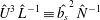 $\hat{U} ^{3}\,\hat{L}^{-1}\equiv \hat{b_{s}}^{2}\,\hat{N}^{-1}$
.

The proposed DNS results, in particular the TKE and MKE budgets, and the role of turbulence isotropization via pressure fluctuations can be used to guide improvements in current turbulence closure modelling for sloping and stable conditions that can then be implemented in the next generation of large-scale atmospheric models.
Appendix A. Sensitivity of solutions to variations in the Grashof number
A.1 Mean flow, TKE and buoyancy variance
The sensitivity of mean velocity and buoyancy profiles to variations in
 $Gr$
is displayed in figure 16 for anabatic and katabatic flow regimes characterized by
 $\unicode[STIX]{x1D6FC}=60^{\circ }$
. Increases in
 $Gr$
results in weaker thermal and dynamic boundary layers, i.e. in a decrease of
 $z_{j},u_{j},\unicode[STIX]{x1D6FF}$
, as well as
 $\int _{0}^{H}\langle b\rangle \,\text{d}z$
and
 $\int _{0}^{H}\langle u\rangle \,\text{d}z$
. As apparent from figure 17, increases in
 $Gr$
results in a decrease in the surface buoyancy flux
 $\langle \unicode[STIX]{x1D70F}_{bz}\rangle |_{z=0}$
, i.e. in a reduction of the rate of potential energy that is supplied to the system, as could have been intuitively predicted. Surface momentum fluxes are also decreasing as
 $Gr$
increases, as also displayed in figure 17. Conversely, the magnitude of slope-normal surface gradients of along-slope velocity and buoyancy are stronger as
 $Gr$
increases, highlighting a relatively stronger momentum (buoyancy) replenishment (extraction) induced by turbulent fluctuations. Therefore as
 $Gr$
increases, the LLJ becomes weaker but better mixed.
Sensitivity of TKE budget terms to
 $Gr$
for the katabatic (a,c) and the anabatic (b,d) flow regimes at
 $\unicode[STIX]{x1D6FC}=60^{\circ }$
. Profiles correspond to
 $\mathit{Gr}=5\times 10^{10}$
(dot-dashed lines),
 $\mathit{Gr}=1\times 10^{11}$
(dashed lines), and
 $\mathit{Gr}=2.1\times 10^{11}$
(solid lines). The
 $z$
-axis represents the slope-normal coordinate direction. The location of the LLJ is highlighted with dotted black lines for the various runs, to provide a reference height (note that as
 $Gr$
increases the LLJ height decreases). All terms are normalized by
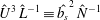 $\hat{U} ^{3}\,\hat{L}^{-1}\equiv \hat{b_{s}}^{2}\,\hat{N}^{-1}$
.

The relatively stronger role of turbulent fluctuations in the near-wall regions as
 $Gr$
increases is apparent if one focuses on figure 18, where TKE and buoyancy variance are featured for both flow regimes. Higher
 $Gr$
results in stronger near-wall TKE and
 $\langle b^{\prime }b^{\prime }\rangle$
, despite the relatively lower kinetic and potential energy of the system, when compared to the same simulation at lower
 $Gr$
. Worth noting also how the near-surface peak of
 $\langle b^{\prime }b^{\prime }\rangle$
is insensitive to
 $Gr$
. This behaviour is in line with findings from mean profiles, which suggest a stronger role of turbulent fluctuations in the near-wall region as
 $Gr$
increases. In the above-LLJ regions TKE,
 $\langle b^{\prime }b^{\prime }\rangle$
and the slope-normal scale of the flow increase in magnitude as
 $Gr$
is reduced for all the considered cases, likely due to the relatively stronger dynamic and thermal boundary layers.
A.2 MKE and TKE budget terms
The dependence of MKE budget terms on
 $Gr$
is highlighted in figure 19. Besides the expected decrease in the slope-normal scale as
 $Gr$
increases, one of the main features of the MKE budget terms is a relative strengthening of
 ${\mathcal{P}}_{s}$
and
 ${\mathcal{T}}_{t}$
in the below-LLJ regions as
 $Gr$
increases. With this regard, note how the peak value of
 ${\mathcal{P}}_{b}$
and
 $\unicode[STIX]{x1D716}_{s}$
are sensitive to variations in
 $Gr$
, whereas the peak value of
 ${\mathcal{P}}_{s}$
and
 ${\mathcal{T}}_{t}$
are insensitive to
 $Gr$
.
As
 $Gr$
increases, TKE budget terms are characterized by a strengthening of
 $P_{s}$
in the neighbourhood of the LLJ and near-surface regions for the katabatic flow regimes (see figure 20). Anabatic flows are instead characterized by a strengthening of
 $P_{s}$
in the near-wall regions, well below
 $z_{j}$
. In addition, buoyant production
 $P_{b,1}$
increases as
 $Gr$
increases in the below LLJ regions and transport terms tend to decrease. This suggests that at higher
 $Gr$
when compared to those considered herein, anabatic and katabatic flows might be characterized by a relatively important local TKE production rate in the below-LLJ regions, and negligible TKE transport rates, ultimately resulting in stronger TKE, and thus larger
 $z_{j}$
and well-mixed profiles of buoyancy and velocity. Such a region might well be the equivalent of the overlap (logarithmic) layer in canonical wall-bounded turbulent flows, which is not observed here, probably because of the relatively low
 $Gr$
values.



