





1. Introduction
Since the discovery of near-wall coherent structures (Klebanoff et al. Reference Klebanoff, Tidstrom and Sargent1962; Kline et al. Reference Kline, Reynolds, Schraub and Runstadler1967; Kim et al. Reference Kim, Kline and Reynolds1971; Smith & Metzler Reference Smith and Metzler1983; Kim et al. Reference Kim, Moin and Moser1987; Robinson Reference Robinson1991; Jeong et al. Reference Jeong, Hussain, Schoppa and Kim1997; Panton Reference Panton2001), the near-wall region has received extensive attention due to its significant contributions to turbulent kinetic energy (TKE) (Kim et al. Reference Kim, Kline and Reynolds1971, Reference Kim, Moin and Moser1987), Reynolds shear stress (Bernard et al. Reference Bernard, Thomas and Handler1993; Schoppa & Hussain Reference Schoppa and Hussain2002) and wall shear stress (Kravchenko et al. Reference Kravchenko, Choi and Moin1993; Fukagata et al. Reference Fukagata, Iwamoto and Kasagi2002). Over the past four decades, motivated by the goal of developing accurate models for the near-wall region and effective control strategies for wall-bounded turbulence, numerous studies have focused on the kinematic characteristics of near-wall coherent structures (Kline et al. Reference Kline, Reynolds, Schraub and Runstadler1967; Smith & Metzler Reference Smith and Metzler1983; Robinson Reference Robinson1991; Jeong et al. Reference Jeong, Hussain, Schoppa and Kim1997; Adrian Reference Adrian2007; Jiménez Reference Jiménez2018) and the underlying mechanisms that sustain near-wall turbulence (Hamilton et al. Reference Hamilton, Kim and Waleffe1995; Waleffe Reference Waleffe1997; Jiménez & Pinelli Reference Jiménez and Pinelli1999; Panton Reference Panton2001; Schoppa & Hussain Reference Schoppa and Hussain2002; Jiménez Reference Jiménez2018; Lozano-Durán et al. Reference Lozano-Durán, Constantinou, Nikolaidis and Karp2021). Given that near-wall turbulence is characterised by complex nonlinear interactions among motions spanning a wide range of length scales (Toh & Itano Reference Toh and Itano2005; Mathis et al. Reference Mathis, Hutchins and Marusic2009; Marusic et al. Reference Marusic, Mathis and Hutchins2010; Hwang et al. Reference Hwang, Lee, Sung and Zaki2016; Hwang & Sung Reference Hwang and Sung2017; Marusic et al. Reference Marusic, Baars and Hutchins2017; McKeon Reference McKeon2017; Cho et al. Reference Cho, Hwang and Choi2018; Hu & Zheng Reference Hu and Zheng2018; Liu et al. Reference Liu, Wang and Zheng2019; Marusic & Monty Reference Marusic and Monty2019; Hu et al. Reference Hu, Yang and Zheng2020; Zhou et al. Reference Zhou, Xu and Jiménez2022; Feng et al. Reference Feng, Liu and Zheng2024; Ma et al. Reference Ma, Xu, Sung, Tian and Huang2025), including near-wall coherent structures (like long streamwise streaks and short quasi-streamwise vortices) and the near-wall footprints of wider attached eddies (Townsend Reference Townsend1976; Perry & Marusic Reference Perry and Marusic1995; Marusic et al. Reference Marusic, Mathis and Hutchins2010; Jiménez Reference Jiménez2012; Hwang Reference Hwang2015; Marusic & Monty Reference Marusic and Monty2019; Motoori & Goto Reference Motoori and Goto2021), an important step towards revealing the key physical processes among these complex nonlinear interactions is to identify the length scales, especially the spanwise length scales, of turbulent motions essential for sustaining near-wall coherent structures and to elucidate their dynamical roles. Such insight can provide a foundation for a more comprehensive understanding of the underlying sustaining mechanisms of near-wall turbulence and the improvement of control strategies.
Minimal flow units proposed by Jiménez & Moin (Reference Jiménez and Moin1991) have been widely used as an effective numerical tool to identify coherent structures and the associated physical processes essential for maintaining wall-bounded turbulence (Hamilton et al. Reference Hamilton, Kim and Waleffe1995; Jiménez & Pinelli Reference Jiménez and Pinelli1999; Schoppa & Hussain Reference Schoppa and Hussain2002; McKeon Reference McKeon2017; Jiménez Reference Jiménez2018; Lozano-Durán et al. Reference Lozano-Durán, Constantinou, Nikolaidis and Karp2021). Minimal flow units originally refer to the smallest computational domains capable of maintaining wall-bounded turbulence in direct numerical simulation (DNS) (Jiménez & Moin Reference Jiménez and Moin1991). Their streamwise and spanwise domain sizes are approximately
 $L_x^+ \approx 350$
and
 $L_z^+ \approx 100$
, respectively, such that each minimal flow unit contains only a single long streak and a few relatively short streamwise vortices. Here, the superscript ‘
 $+$
’ denotes the normalisation based on the friction velocity
 $u_\tau$
and the kinematic viscosity
 $\nu$
, while the subscripts ‘
 $x$
’ and ‘
 $z$
’ refer to the streamwise and spanwise directions, respectively. Compared with the full-scale DNS of wall-bounded turbulence in a large computational domain, the number of degrees of freedom in the spectral space is significantly reduced. For example, for the DNS using the spectral method, reducing the spanwise domain size from
 $L_z$
to
 $L_z/m$
(where
 $m \gg 1$
) retains only the spanwise wavenumbers
 $k_z = 2\pi m n / L_z$
(with integer
 $n = 0, 1, 2, \ldots$
) from the original set
 $k_z = 2\pi n / L_z$
, while all others are filtered out. Consequently, within a standard minimal flow unit, turbulent motions wider than
 $100$
wall units are not resolved, except for the spanwise-uniform components. This spectral sparsity greatly simplifies nonlinear interactions in wall-bounded turbulence, making the minimal flow unit a powerful tool for studying the dynamics of near-wall turbulence.
With the advantage of minimal flow units, a consensus has emerged that near-wall turbulence can sustain itself through a quasi-periodic cycle independent of turbulent motions in the outer layer (Hamilton et al. Reference Hamilton, Kim and Waleffe1995; Jiménez & Pinelli Reference Jiménez and Pinelli1999; Schoppa & Hussain Reference Schoppa and Hussain2002; Jiménez Reference Jiménez2018). This self-sustaining cycle consists of three key processes (Hamilton et al. Reference Hamilton, Kim and Waleffe1995; Waleffe Reference Waleffe1997; Jiménez & Pinelli Reference Jiménez and Pinelli1999; Panton Reference Panton2001; Schoppa & Hussain Reference Schoppa and Hussain2002): the generation of long streaks by streamwise vortices via the lift-up effect (Butler & Farrell Reference Butler and Farrell1993; Reddy & Henningson Reference Reddy and Henningson1993; Reddy et al. Reference Reddy, Schmid, Baggett and Henningson1998; Schmid & Henningson Reference Schmid and Henningson2001; del Álamo & Jiménez Reference del Álamo and Jiménez2006; Schmid Reference Schmid2007; Pujals et al. Reference Pujals, García-Villalba, Cossu and Depardon2009; Jiménez Reference Jiménez2013), the breakdown of long streaks due to the linear instability or the linear transient growth (Waleffe Reference Waleffe1997; Schoppa & Hussain Reference Schoppa and Hussain2002; Jiménez Reference Jiménez2013; Lozano-Durán et al. Reference Lozano-Durán, Constantinou, Nikolaidis and Karp2021) and the regeneration of short streamwise vortices through the nonlinear vortex stretching (Hamilton et al. Reference Hamilton, Kim and Waleffe1995; Schoppa & Hussain Reference Schoppa and Hussain2002). This theoretical framework has also been extended to explain the maintenance of coherent structures in the logarithmic layer at moderate to high Reynolds numbers (Flores & Jiménez Reference Flores and Jiménez2010; Hwang & Cossu Reference Hwang and Cossu2011; Hwang & Bengana Reference Hwang and Bengana2016; Lozano-Durán et al. Reference Lozano-Durán, Bae and Encinar2020). Jiménez & Pinelli (Reference Jiménez and Pinelli1999) have demonstrated in minimal flow units that suppressing any of these three processes or the fundamental elements within the cycle leads to the relaminarisation of wall-bounded turbulence. The self-sustaining cycle highlights the critical role of the interaction between long streaks and short vortices, representative of nonlinear interactions among different streamwise length scales, in maintaining near-wall turbulence.
Recently, it has been discovered that nonlinear interactions filtered out in minimal flow units also play a significant role in maintaining near-wall turbulence. Jiménez (Reference Jiménez2022) revisited the interdependence between long streaks and short vortical structures through numerical experiments in full-scale DNS, and demonstrated that near-wall turbulence can be maintained by self-interaction of short vortical structures in the absence of long streaks. Meanwhile, in the study using the generalised quasilinear (GQL) analysis (Hernández et al. Reference Hernández, Yang and Hwang2022a ), it has been found that short turbulent motions can be maintained by the nonlinear interaction between long and short turbulent motions, even though the nonlinear stretching induced by the self-interaction among short turbulent motions is absent. In addition, the opposition control (Choi et al. Reference Choi, Moin and Kim1994) can induce the relaminarisation of minimal channel flows by suppressing the generation of long streaks and short streamwise vortices (Deng & Xu Reference Deng and Xu2012; Deng et al. Reference Deng, Xu, Huang and Cui2013), while wall-bounded turbulence remains sustained in full-scale DNS despite weakened near-wall coherent structures (Choi et al. Reference Choi, Moin and Kim1994; Hammond et al. Reference Hammond, Bewley and Moin1998; Chung & Talha Reference Chung and Talha2011; Sonoda et al. Reference Sonoda, Liu, Itoh and Hasegawa2023). These findings suggest that, in addition to the classical self-sustaining cycle, different potential mechanisms for the maintenance of near-wall turbulence co-exist when the number of degrees of freedom is increased and the associated nonlinear interactions become more complex in full-scale DNS. Therefore, a reassessment of the length scales of turbulent motions essential for maintaining near-wall turbulence in full-scale DNS is needed.
In the aforementioned study mainly focusing on the complex nonlinear interaction among different streamwise length scales (Hernández et al. Reference Hernández, Yang and Hwang2022a
; Jiménez Reference Jiménez2022), all spanwise length scales were retained. In the near-wall region, there exist turbulent motions across a broad range of spanwise wavelengths, largely attributed to the near-wall footprints of self-similar attached eddies (Townsend Reference Townsend1976; Perry & Chong Reference Perry and Chong1982; Perry & Marusic Reference Perry and Marusic1995; Hoyas & Jiménez Reference Hoyas and Jiménez2006; Hutchins & Marusic Reference Hutchins and Marusic2007a
; Mathis et al. Reference Mathis, Hutchins and Marusic2009; Marusic et al. Reference Marusic, Mathis and Hutchins2010; Jiménez Reference Jiménez2012; Lozano-Durán & Jiménez Reference Lozano-Durán and Jiménez2014; Hwang Reference Hwang2015, Reference Hwang2016; Agostini & Leschziner Reference Agostini and Leschziner2017; Baars et al. Reference Baars, Hutchins and Marusic2017; Marusic & Monty Reference Marusic and Monty2019; Andreolli et al. Reference Andreolli, Gatti, Vinuesa, Örlü and Schlatter2023). Self-similar attached eddies are defined as turbulent structures whose characteristic length scales and vertical extents increase with the distance of their centres from the wall (Jiménez Reference Jiménez2012; Hwang Reference Hwang2015). For a given spanwise wavelength
 $\lambda _z$
ranging from
 $100$
wall units to
 $1.5h$
(where
 $h$
denotes the half-channel height), Hwang (Reference Hwang2015) classified these eddies into two distinct types. The first type consists of long streaks that exhibit strong streamwise velocity fluctuations and follow self-similar scalings,
 $\lambda _x \approx 10\,\lambda _z$
and
 $y \approx 0.1\,\lambda _z$
. The second type comprises short vortical structures that involve all three velocity components and scale as
 $\lambda _x \approx 2{-}3\,\lambda _z$
and
 $y \approx 0.5{-}0.7\,\lambda _z$
(Hwang Reference Hwang2015). According to the scaling, the classical near-wall streaks and quasi-streamwise vortices, characterised by a typical spanwise spacing of
 $\lambda _z^+ \approx 100$
, can be interpreted as the smallest members of the attached-eddy hierarchy (Hwang Reference Hwang2015). Notably, in the numerical experiments of Jiménez (Reference Jiménez2022), the flow relaminarises when turbulent motions with streamwise wavelengths longer than
 $600$
viscous units were all artificially damped. This critical threshold,
 $\lambda _x^+ = 600$
, corresponds to a spanwise scale of
 $\lambda _z^+ \approx 200{-}300$
, based on the self-similar scaling relations for vortical attached eddies (Hwang Reference Hwang2015). Furthermore, using the GQL approximation in the spanwise direction, Hernández et al. (Reference Hernández, Yang and Hwang2022b
) demonstrated that nonlinear interactions between spanwise-wide and spanwise-narrow turbulent motions can feed spanwise-narrow turbulent motions in the absence of direct nonlinear interactions between long and short turbulent motions, although the spectra of these spanwise-narrow motions differ from those obtained from large-eddy simulations. These findings suggest that turbulent motions with spanwise scales larger than those of canonical near-wall coherent structures also contribute to maintaining near-wall turbulence.
Nonlinear interactions among turbulent motions of different spanwise length scales have also been observed to participate in the energy transfer processes within the near-wall region. Doohan et al. (Reference Doohan, Willis and Hwang2021) found that vertical turbulent transport from motions around
 $\lambda _z^+ = 200$
to those around
 $\lambda _z^+ = 110$
in the near-wall region can drive turbulent production around
 $\lambda _z^+ = 110$
via the Orr mechanism (Orr Reference Orr1907; Jiménez Reference Jiménez2013, Reference Jiménez2015; Jiao et al. Reference Jiao, Hwang and Chernyshenko2021). Studies of energy spectral budgets by Mizuno (Reference Mizuno2016), Cho et al. (Reference Cho, Hwang and Choi2018) and Lee & Moser (Reference Lee and Moser2019) further show that the vertical component of TKE is transported downward to
 $y^+ \approx 40$
and subsequently transferred to smaller spanwise scale. Furthermore, Kawata & Tsukahara (Reference Kawata and Tsukahara2021) compared the spectral energy budgets of full-scale DNS and spanwise-minimal DNS, revealing that the aggregate contribution of turbulent motions with
 $\lambda _z^+ \gt 110$
to energy transfer in full-scale simulations is analogous to that of spanwise-uniform motions in minimal flow units.
Despite the above-mentioned findings about the contribution of nonlinear interaction among different spanwise length scales, turbulent motions in which specific spanwise length scales are essential to maintaining near-wall turbulence and the dynamical mechanisms explaining why they are necessary remain unclear. To address these two questions, we perform numerical experiments based on a full-scale DNS, in which turbulent motions at large spanwise length scales are damped. This filter removes the contribution of spanwise-wide motions to near-wall coherent structures while preserving self-interaction among short vortical structures, the self-interactions among long streaks, and the nonlinear interactions between long streaks and short vortices. This approach enables us to identify the specific spanwise length scales required to sustain near-wall turbulence, similar to that used by Jiménez (Reference Jiménez2022) for studying the necessity of long streaks. Furthermore, we separately analyse the budgets of Reynolds stresses associated with near-wall long streaks and short vortical structures, and decompose the nonlinear transport term to isolate the contribution arising from nonlinear interactions involving spanwise-wide turbulent motions. This decomposition reveals distinct dynamical roles of spanwise-wide motions in the maintenance of long streaks and short vortical structures, thereby elucidating why these spanwise-wide turbulent motions are essential for maintaining near-wall turbulence.
The remainder of the paper is organised as follows. The numerical set-up is described in detail in § 2. In § 3, we identify the range of spanwise length scales of turbulent motions essential for sustaining near-wall turbulence. We present the responses of turbulent statistics and coherent structures to the artificial filter in § 4, highlighting the contrasting effects of spanwise-wide motions on long streaks and short vortical structures. In § 5, we further examine the underlying mechanisms by analysing the budget terms of Reynolds stresses contributed separately by long streaks and short vortical structures, and their responses in numerical experiments, which provides a summary of the multiple energy cycles feeding them. Then, the near-wall energy cycles and the responses of near-wall turbulence to numerical experiments are confirmed at a higher Reynolds number in § 6. Finally, conclusions are provided in § 7.
2. Computational methodology of numerical experiments
To identify the spanwise length scales of turbulent motions essential for sustaining near-wall turbulence and to elucidate their dynamical roles, we conduct numerical experiments based on full-scale DNS of incompressible turbulent channel flow with a constant mass flux driven by a streamwise pressure gradient. This section first introduces the numerical methods employed in our DNS and then describes the set-up of the numerical experiments.
2.1. Numerical methods of DNS
The governing equations for the incompressible turbulent channel flow include the continuity equation
 \begin{equation} \frac { \partial u_i}{ \partial x_i} = 0, \end{equation}
and the momentum equation
 \begin{equation} \frac { \partial u_i}{ \partial t} +\frac {\partial u_i u_{\!j}}{\partial x_{\!j}}= -\frac {1}{\rho }\frac { \partial p}{ \partial x_i} + \nu \frac {\partial ^2 u_i}{\partial x_{\!j} \partial x_{\!j}}. \end{equation}
In (2.1) and (2.2),
 $p$
denotes the pressure,
 $\rho$
is the density and
 $\nu$
is the kinematic viscosity. The velocity
 $u_i$
comprises three velocity components
 $u_1=u$
,
 $u_2=v$
and
 $u_3=w$
, corresponding to the velocity components in the streamwise (
 $x$
), vertical (
 $y$
) and spanwise (
 $z$
) directions, respectively.
Equations (2.1) and (2.2) are solved using a hybrid finite-differential/spectral method. The velocity is expanded in Fourier series in the periodic streamwise (
 $x$
) and spanwise (
 $z$
) directions as
 \begin{equation} u_i(x,y,z,t) = \sum _{k_x} \sum _{k_z} \widehat {u}_i(k_x,y,k_z,t) \exp {[i(k_x x + k_z z)]}, \end{equation}
where
 $k_x$
and
 $k_z$
denote the streamwise and spanwise wavenumbers, respectively, and
 $\widehat {u}_i$
represents the Fourier coefficient of
 $u_i$
. In the vertical (
 $y$
) direction, a staggered grid is employed. The streamwise velocity (
 $u$
), spanwise velocity (
 $w$
) and pressure (
 $p$
) are defined at cell centres, while the vertical velocity (
 $v$
) is located at cell faces. A sixth-order compact finite-differential scheme is used for spatial discretisations in the
 $y$
-direction. No-slip boundary conditions are imposed at the two walls located at
 $y = \pm h$
. Time integration is advanced using a third-order Runge–Kutta (RK3) scheme.
Within each RK3 substep, a fractional-step method is employed to enforce the divergence-free condition given by (2.1). In the spectral space, each substep of the RK3 scheme consists of the following three stages:
 \begin{equation} \big(\Delta t^{-1} - \beta _l L\big)\widehat {u}_i^* = \Delta t^{-1}\widehat {u}_i^{l-1} - \gamma _l \widehat {C}\big(u_i^{l-1}\big) - \eta _l \widehat {C}\big(u_i^{l-2}\big) + \beta _l L\big(\widehat {u}_i^{l-1}\big), \end{equation}
 \begin{equation} \Delta t \delta _l \frac {1}{\rho } \textit{DG} \widehat {p}^l = \frac {\partial \widehat {u}_i^*}{\partial x_i} \end{equation}
and
 \begin{equation} \widehat {u}_i^l = \widehat {u}_i^* - \Delta t \delta _l \frac {\partial \widehat {p}^l}{\rho \partial x_i}. \end{equation}
Here,
 $l = 1, 2$
and
 $3$
denotes the substep index of the RK3 scheme. The coefficients are given by
 \begin{align} & \beta _1 = \frac {4}{15},\quad \beta _2 = \frac {1}{15},\quad \beta _3 = \frac {1}{6}, \end{align}
 \begin{align} & \gamma _1 = \frac {8}{15},\quad \gamma _2 = \frac {5}{12},\quad \gamma _3 = \frac {3}{4}, \end{align}
 \begin{align} &\quad \,\, \eta _1 = 0,\quad \eta _2 = -\frac {17}{60},\quad \eta _3 = -\frac {5}{12}, \end{align}
 \begin{align} & \delta _1 = \frac {8}{15},\quad \delta _2 = \frac {2}{15},\quad \delta _3 = \frac {1}{3}. \end{align}
For
 $l=1$
and
 $3$
, the velocities
 $u_i^0$
and
 $u_i^3$
represent the flow fields at the
 $n{\mathrm{th}}$
and
 $(n+1){\mathrm{th}}$
time steps, respectively, separated by a time interval
 $\Delta t$
. Here,
 $D$
and
 $G$
represent the divergent and gradient operators, respectively. The term
 $L(\widehat {u}_i)$
denotes the Fourier coefficient of the viscous term
 $\partial ^2 u_i / (\partial x_{\!j} \partial x_{\!j})$
in (2.2). The term
 $\widehat {C}(u_i)$
represents the Fourier coefficient of the nonlinear convection term
 $\partial (u_i u_{\!j})/\partial x_{\!j}$
in (2.2), which is expressed as
 \begin{equation} \widehat {C}(u_i)(k_x,y,k_z,t) = i k_x \widehat {u_iu_{\!j}} \delta _{1j} + \frac {\partial \widehat {u_iu_{\!j}}}{\partial y} \delta _{2j} + i k_z \widehat {u_iu_{\!j}}\delta _{3j}. \end{equation}
For given wavenumbers
 $k_{x0}$
and
 $k_{z0}$
, the Fourier coefficient
 $\widehat {u_i u_{\!j}}$
is equal to
 \begin{equation} \widehat {u_i u_{\!j}}(k_{x0},y,k_{z0}) = \sum _{k_x, k_z} \widehat {u}_i (k_x,y, k_z) \widehat {u}_{\!j} (k_{x0}-k_x,y, k_{z0}-k_z), \end{equation}
which explicitly accounts for the triadic nonlinear interactions among turbulent motions across different length scales. The
 $3/2$
rule is employed to remove the aliasing errors in the nonlinear terms (Kravchenko & Moin Reference Kravchenko and Moin1997). Our numerical tool has been validated in our previous studies, such as opposition control of turbulent channel flows (Deng & Xu Reference Deng and Xu2012; Deng et al. Reference Deng, Huang and Xu2016), coherent structures in rotating channel flows (Yang & Wang Reference Yang and Wang2018; Yang et al. Reference Yang, Deng, Wang and Shen2020) and open channel flows driven by surface shear stresses (Deng et al. Reference Deng, Yang, Xuan and Shen2019, Reference Deng, Yang, Xuan and Shen2020; Deng et al. Reference Deng, Yang and Shen2022).
2.2. Set-up of numerical experiments
According to Hwang (Reference Hwang2015) and Marusic & Monty (Reference Marusic and Monty2019), energetic attached eddies are composed of self-similar long streaks and short vortical structures, with their vertical height growing with their length scales. Crucially, long streaks and short vortices sharing the same spanwise length scale form a self-sustaining unit (Hwang Reference Hwang2015; Cossu & Hwang Reference Cossu and Hwang2017), the smallest of which corresponds to the near-wall cycle. Therefore, to reveal the dependence of near-wall turbulent motions on other wider ones, we designed numerical experiments to suppress the spanwise-wide turbulent motions. Specifically, in fully developed turbulent channel flows, all three velocity components with their spanwise wavelength satisfying
 $\lambda _z = 2\pi / |k_z| \gt \lambda _{zf}$
are set to zero after a prescribed time
 $t_0$
. This high-pass spectral filter is defined as
 \begin{equation} \widehat {u}_i^l(k_x, y, k_z, t \geqslant t_0) = 0 \quad \text{for} \quad |k_z| \lt k_{zf} = \frac {2\pi }{\lambda _{zf}} \quad \text{and} \quad k_x^2 + k_z^2 \neq 0, \end{equation}
where
 $k_{zf}$
denotes the cutoff spanwise wavenumber corresponding to the cutoff spanwise wavelength
 $\lambda _{zf}$
. Here, the high-pass filter is not applied in the streamwise wavenumbers. This is because, among numerous established numerical experiments (Hamilton et al. Reference Hamilton, Kim and Waleffe1995; Jiménez & Pinelli Reference Jiménez and Pinelli1999; Hwang Reference Hwang2013; Bae et al. Reference Bae, Lozano-Durán and McKeon2021; Jiménez Reference Jiménez2022), those suppressing long structures (Hamilton et al. Reference Hamilton, Kim and Waleffe1995; Jiménez & Pinelli Reference Jiménez and Pinelli1999; Jiménez Reference Jiménez2022) were typically employed to investigate the dependence of short vortical structures on long streaks, a topic that lies beyond the scope of this study.
The filter defined in (2.13) is applied after the prediction step (2.4) and prior to the projection step (2.5) within each RK3 substep. This sequence ensures mass conservation. For the mean flow and turbulent motions at retained wavelengths, the momentum is strictly conserved, as they are obtained by solving the momentum equation in the spectral space. For turbulent motions suppressed at the targeted wavenumbers, i.e.
 $|k_z|\lt k_{zf}$
in this study, the momentum is removed at every step. Such methodology, which directly removes the momentum at specified wavenumbers, has been used in numerous established numerical experiments to investigate the sustaining mechanism of wall-bounded turbulence (Hamilton et al. Reference Hamilton, Kim and Waleffe1995; Jiménez & Pinelli Reference Jiménez and Pinelli1999; Hwang Reference Hwang2013; Bae et al. Reference Bae, Lozano-Durán and McKeon2021; Jiménez Reference Jiménez2022). For instance, in the numerical experiments of Hwang (Reference Hwang2013), the right-hand side of the prediction step (2.4) was set to zero for the specified wavenumbers to remove the momentum at these length scales, which yields an effect equivalent to our filter. We have successfully replicated the numerical experiments of Hwang (Reference Hwang2013) and Jiménez (Reference Jiménez2022) in Appendix A. The close agreement between our results and theirs validates the effectiveness and robustness of the current approach in suppressing turbulent motions within the targeted wavenumber range.
Using the spanwise filter in (2.13), the internal nonlinear interactions for turbulent motions with
 $\lambda _z \leqslant \lambda _{zf}$
are retained, while all contributions from wider turbulent motions with
 $\lambda _z \gt \lambda _{zf}$
through triadic nonlinear interactions (2.11)–(2.12), i.e. the ‘scattering’ mechanism (Tobias & Marston Reference Tobias and Marston2017; Hernández et al. Reference Hernández, Yang and Hwang2022b
), are eliminated. In particular, when
 $\lambda _{zf}^+ \gt 110$
, nonlinear interactions among canonical near-wall long streaks and short streamwise vortices in the self-sustaining cycle (Hamilton et al. Reference Hamilton, Kim and Waleffe1995; Waleffe Reference Waleffe1997; Jiménez & Pinelli Reference Jiménez and Pinelli1999; Panton Reference Panton2001; Schoppa & Hussain Reference Schoppa and Hussain2002) and the self-bursting process (Jiménez Reference Jiménez2022) are preserved. By changing the values of
 $\lambda _{zf}$
and monitoring the flow state, one can determine the threshold value of
 $\lambda _{zf}$
, i.e. the minimal value
 $\lambda _{zf}^{\textit{min}}$
to maintain near-wall turbulence, regardless of whether the maintenance of near-wall coherent structures is dominated by the canonical self-sustaining cycle or the recently proposed self-bursting process.
Since this study focuses on the near-wall region, our analyses are primarily based on numerical experiments conducted at a relatively low bulk Reynolds number
 $\textit{Re}_m = U_m h / \nu = 2800$
, where
 $U_m$
denotes the bulk mean velocity. In the undamped (UnD) case, i.e. without application of the spectral filter (2.13), the corresponding friction Reynolds number is
 $\textit{Re}_\tau = u_\tau h / \nu \approx 180$
. To achieve a precise estimation of the spanwise length scales critical for near-wall turbulence, full-scale DNS is performed in a computational domain size of
 $L_x \times L_y \times L_z = 4\pi h \times 2h \times 2\pi h$
. This domain size is significantly larger than a minimal flow unit (Jiménez & Moin Reference Jiménez and Moin1991; Jiménez & Pinelli Reference Jiménez and Pinelli1999), thereby enabling a denser distribution of the discrete spanwise wavelengths in the spectral space and allowing for finer resolution of the critical spanwise length scales. A grid of
 $192 \times 128 \times 192$
is employed, corresponding to the grid spacings of
 $\Delta x^+ \approx 11.8$
,
 $\Delta z^+ \approx 5.9$
and
 $\Delta y^+_{\textit{min}} \approx 0.13$
. Hereinafter, the superscript ‘+’ represents the normalisation using the friction velocity
 $u_\tau$
in the case UnD. In this study, several values of the cutoff spanwise wavelength
 $\lambda _{zf}$
are considered to determine
 $\lambda _{zf}^{\textit{min}}$
, as listed in table 1. Additional numerical experiments at a higher Reynolds number
 $\textit{Re}_m = 11\,000$
(corresponding to
 $\textit{Re}_\tau \approx 590$
) are also conducted to discuss the Reynolds number dependence of the critical cutoff wavelength
 $\lambda _{zf}^{\textit{min}}$
for sustaining near-wall turbulence in § 6.
Parameters of numerical experiments at a fixed bulk Reynolds number
 $\textit{Re}_m = 2800$
. Here,
 $\lambda _{zf}$
denotes the cutoff spanwise wavelength in the high-pass spectral filter (2.13) and
 $\textit{Re}_\tau$
is the friction Reynolds number in different cases. The superscript ‘+’ denotes the normalisation using the kinematic viscosity
 $\nu$
and the friction velocity
 $u_\tau$
in the undamped (UnD) case.

Table 1. Long description
The table presents parameters of numerical experiments at a fixed bulk Reynolds number. It includes seven rows and eleven columns. The columns are labeled as follows: Case, Re_m, L_x x L_y x L_z, Delta x+, Delta y_min+, Delta z+, lambda_z_c+, lambda_z_c/h, Re_t, and Flow state. The rows are labeled with different cases: UnD, DZ01, DZ02, DZ03, DZ04, and DZ05. Each row provides specific values for each parameter. For example, Row 1: UnD, 2800, 4 pi h x 2 h x 2 pi h, 11.8, 0.13, 5.9, 565, 3.14, 178.9, Fully turbulent. Row 2: DZ01, 2800, 4 pi h _ 2 h _ 2 pi h, 11.8, 0.13, 5.9, 376, 2.09, 177.6, Turbulent. Row 3: DZ02, 2800, 4 pi h _ 2 h _ 2 pi h, 11.8, 0.13, 5.9, 282, 1.57, 176.2, Turbulent. Row 4: DZ03, 2800, 4 pi h x 2 h x 2 pi h, 11.8, 0.13, 5.9, 226, 1.26, 155.2, Transitional. Row 5: DZ04, 2800, 4 pi h x 2 h x 2 pi h, 11.8, 0.13, 5.9, 188, 1.05, 66.4, Relaminarising.
3. Spanwise length scales essential for near-wall turbulence
In this section, we identify the spanwise length scales of turbulent motions necessary for sustaining turbulent channel flows by examining the flow states in our numerical experiments listed in table 1.
Time histories of (a) the horizontally averaged wall shear stress
 $\tau _w$
and (b) the bulk-averaged TKE
 $E= \int _0^{L_x}\int _{-h}^h \int _{0}^{L_z}0.5 u_i^\prime u_i^\prime \,{\rm d}x\,{\rm d}y\,{\rm d}z/(2hL_xL_z)$
in the numerical experiments of turbulent channel flows listed in table 1. Here,
 $\tau _w$
is normalised by
 $\rho U_m^2$
, while
 $E$
is normalised by the friction velocity
 $u_{\tau }^2$
in the case UnD. All the simulations are initialised from a fully developed turbulent channel flow field at the same instant
 $t=t_0$
. The results in a minimal channel with its spanwise domain size limited to
 $L_z^+=188$
are also shown (the case Mini).

Figure 1. Long description
Two line graphs depict the time histories of wall shear stress and turbulent kinetic energy in numerical experiments of turbulent channel flows. Panel A: The line graph shows the horizontally averaged wall shear stress. The x-axis represents the dimensionless time ((t − t0)Um/h) ranging from 0 to 300, and the y-axis represents the normalized wall shear stress (τw/ρUm^2) ranging from 0 to 5 times 10^−3. Different lines represent various cases with different damping parameters. Panel B: The line graph shows the bulk-averaged turbulent kinetic energy. The x-axis represents the dimensionless time ((t − t0)Um/h) ranging from 0 to 300, and the y-axis represents the normalized turbulent kinetic energy (E+) ranging from 0 to 3. Different lines represent various cases with different damping parameters. The legend indicates the specific parameters for each case.
Figure 1 shows the time histories of the horizontally averaged wall shear stress
 $\tau _w$
and the bulk-averaged TKE
 $E= \int _0^{L_x}\int _{-h}^h \int _{0}^{L_z}0.5 u_i^\prime u_i^\prime \, {\rm d}x{\rm d}y{\rm d}z/(2hL_xL_z)$
in numerical experiments DZ01–DZ05 at
 $\textit{Re}_m = 2800$
. For comparison, the results in the case UnD are included as references. Hereinafter, the superscript ‘
 $\prime$
’ represents turbulent fluctuations. The long-term evolutions of
 $\tau _w$
and
 $E$
can serve as indicators of the flow state. As shown in the cases DZ01–DZ03, where the cutoff spanwise wavelength satisfies
 $\lambda _{zf}^+ \geqslant 282$
(
 $\lambda _{zf}/h \geqslant 1.57$
), both
 $\tau _w$
and
 $E$
remain nearly identical to those in the case UnD. This indicates that wall-bounded turbulence is sustained when
 $\lambda _{zf}^+ \geqslant 282$
, although the features of turbulent motions are altered by the application of the filter (as later shown in § 4). In contrast, for
 $\lambda _{zf}^+ = 226$
(
 $\lambda _{zf}/h = 1.26$
) in the case DZ04,
 $\tau _w$
initially remains close to the value in the case UnD, but subsequently decreases significantly, while the bulk-averaged TKE
 $E$
is suppressed to a value around half of that in the case UnD. This behaviour characterises a transitional state between turbulence and relaminarisation. When the cutoff wavelength is further reduced to
 $\lambda _{zf}^+ = 188$
(
 $\lambda _{zf}/h = 1.05$
) in the case DZ05, a rapid drop in
 $\tau _w$
is observed and
 $E$
decays to zero, indicating the complete relaminarisation of the flow. Therefore,
 $\lambda _{zf}$
must exceed approximately
 $226$
viscous units (or
 $1.26h$
) to maintain a turbulent state.
Notably, at
 $\textit{Re}_m = 2800$
, the separation between the viscous length scale
 $\nu /u_\tau$
and the outer length scale
 $h$
is insufficient to determine whether the critical cutoff wavelength
 $\lambda _{zf}^{\textit{min}}$
scales with the inner or outer length scales. According to the later discussion of the dependence of
 $\lambda _{zf}^{\textit{min}}$
on Reynolds number in § 6, at
 $\textit{Re}_m = 11\,000$
(
 $\textit{Re}_\tau \approx 590$
), the wall-bounded turbulence is still sustained when
 $\lambda _{zf}^+ \gt 200$
(corresponding to
 $\lambda _{zf}/h \gt 0.34$
). This implies that
 $\lambda _{zf}^{\textit{min}}$
scales with the viscous length scale, i.e.
 \begin{equation} \lambda _{zf}^{\textit{min} +} \approx 200, \end{equation}
indicating that at least turbulent motions with spanwise length scales around
 $200$
wall units, twice that of near-wall coherent structures (
 $\lambda _{z}^+\approx 100$
), are necessary to sustain near-wall turbulence.
It should be noted that the threshold spanwise wavelength
 $\lambda _{zf}^+\approx 200$
identified in full-scale DNS should be distinguished from the threshold spanwise domain size of minimal flow units required to sustain near-wall turbulence. To illustrate this, we compare a minimal channel flow with a spanwise domain size
 $L_z^+\approx 188$
against the case DZ05 (with
 $\lambda _{zf}^+=188$
) in full-scale DNS. In the minimal channel, the flow remains turbulent, with its total energy
 $E$
, wall shear stress
 $\tau _w$
(figure 1) and near-wall statistics (figures 3 and 4) close to those of the undamped case (UnD), which is markedly distinct from the relaminarisation observed in the case DZ05. This discrepancy arises because the minimal channel retains spanwise-uniform turbulent motions. According to Kawata & Tsukahara (Reference Kawata and Tsukahara2021), although the minimal channel does not directly resolve motions with
 $L_z\lt \lambda _z\lt \infty$
, the spanwise-uniform motions play a role analogous to the aggregate effect of turbulent motions within this length scale range in full-scale DNS. Actually, the threshold spanwise size of minimal flow units for sustaining turbulence is
 $L_z^+\approx 100$
(Jiménez & Moin Reference Jiménez and Moin1991), but it also undergoes laminarisation when the three velocity components of spanwise-uniform motions are suppressed (see the results in Appendix A), suggesting that the threshold wavelength for sustaining near-wall turbulence lies in the range
 $100\lt \lambda _z^+\leqslant \infty$
. While previous studies have revealed that turbulent motions with
 $\lambda _z^+ \gtrsim 200$
can energise the near-wall regeneration cycle either through the breakup of long streaks (Hamilton et al. Reference Hamilton, Kim and Waleffe1995; Schoppa & Hussain Reference Schoppa and Hussain2002; Hwang Reference Hwang2013; Kawata & Tsukahara Reference Kawata and Tsukahara2021), the linear Orr mechanism (Orr Reference Orr1907; Jiménez Reference Jiménez2013, Reference Jiménez2015; Doohan et al. Reference Doohan, Willis and Hwang2021; Jiao et al. Reference Jiao, Hwang and Chernyshenko2021) or nonlinear scattering processes that redistribute energy from large to small scales (Tobias & Marston Reference Tobias and Marston2017; Hernández et al. Reference Hernández, Yang and Hwang2022b
), this study further confirms the necessity of turbulent motions wider than near-wall coherent structures and provides a refined threshold value for the required spanwise length scales.
(a) Premultiplied spanwise co-spectrum of
 $u^\prime$
and
 $v^\prime$
, denoted as
 $k_zE_{-u^\prime v^\prime }(\lambda _z^+, y^+)$
, in the case UnD; and (b) the integral ratio at different spanwise length scales
 $\sigma _{-u^\prime v^\prime }(\lambda _z^+)$
in the near-wall region defined in (3.2) in the cases UnD–DZ04. The vertical dashed line is located at approximately
 $\lambda _z^+ = 188$
.

Furthermore, it is worth emphasising that turbulent motions with
 $\lambda _z^+\geqslant 200$
are obviously less active than the canonical near-wall coherent structures in terms of their contributions to the Reynolds shear stress in the near-wall region. Figure 2(a) presents the premultiplied spanwise co-spectrum
 $k_zE_{-u^\prime v^\prime }(\lambda _z^+, y^+)$
. As shown in figure 2(a), the spectral peak occurs near
 $y^+=30$
and
 $\lambda _z^+=110$
, confirming that the most energetic contributions arise from near-wall coherent structures. Figure 2(b) further quantifies the contribution of turbulent motions at various spanwise length scales to Reynolds shear stresses in the near-wall region through the cumulative integral ratio
 $\sigma _{-u^\prime v^\prime }(\lambda _z^+)$
defined as
 \begin{equation} \sigma _{-u'v'}(\lambda _z) = \frac {\int _{y^+=0}^{y^+=70} \int _{\lambda _z}^{\infty } E_{-u'v'}(y,\lambda _z)\, \mathrm{d}\lambda _z\, \mathrm{d}y}{\int _{y^+=0}^{y^+=70} -\langle u'v' \rangle\, \mathrm{d}y}. \end{equation}
While the flow relaminarises when
 $\lambda _{zf}^+=188$
(figure 1) at
 $\textit{Re}_m=2800$
, turbulent motions with
 $\lambda _z^+\gt 188$
in the case UnD account for only approximately
 $25\,\%$
of the total Reynolds shear stress in the near-wall region. This ratio further decreases with the reduction of the cutoff wavelength
 $\lambda _{zf}^+$
in cases DZ01–DZ04, suggesting the more significant contribution of near-wall coherent structures. Therefore, it is necessary to further investigate how the absence of these less active spanwise-wide motions impacts near-wall coherent structures and ultimately leads to relaminarisation when
 $\lambda _{zf}^+=188$
, as discussed in the following sections.
4. Response of near-wall turbulence in numerical experiments
In this section, we present a detailed analysis of the response of near-wall turbulence to the high-pass spectral filter (2.13), with the aim of elucidating how spanwise-wide motions influence near-wall coherent structures. For this purpose, the changes in the mean velocity profile and the Reynolds stresses in the numerical experiments are first shown, and then the contrasting responses of near-wall long streaks and short vortical structures in the numerical experiments are revealed through the analyses of energy spectra, Reynolds stresses associated separately with near-wall long streaks and short vortical structures, and instantaneous flow fields.
4.1. Mean velocity and Reynolds stresses
Variations of the profiles of (a) the mean velocity
 $\langle u\rangle ^+$
and (b) the Reynolds shear stress
 $-\langle u' v' \rangle ^+$
with the spanwise cutoff wavelength
 $\lambda _{zf}^+$
at the bulk Reynolds number
 $\textit{Re}_m=2800$
. In the cases DZ01–DZ04,
 $\lambda _{zf}^+$
varies from 565 to 226. The results in a minimal channel with its spanwise domain size limited to
 $L_z^+=188$
are also shown (the case Mini). All profiles are normalised by the friction velocity
 $u_\tau$
in the case UnD.

Figure 3. Long description
Two line graphs depict variations of profiles of mean velocity and Reynolds shear stress with spanwise cutoff wavelength. Panel A: The line graph shows the mean velocity profiles. The x-axis is labeled y+ and ranges from 10^0 to 10^2. The y-axis is labeled <u>+ and ranges from 0 to 20. The graph includes multiple data series represented by different line styles and colors: solid black line for UnD, dashed magenta line for DZ01, dotted blue line for DZ02, dashed blue line for DZ03, dashed orange line for DZ04, and solid green line for Mini. Panel B: The line graph shows the Reynolds shear stress profiles. The x-axis is labeled y+ and ranges from 10^0 to 10^2. The y-axis is labeled −<u’v’>+ and ranges from 0 to 0.9. The graph includes the same data series as Panel A. The profiles are normalized by the friction velocity in the case UnD.
Figure 3 shows the variations of the profiles of the mean velocity
 $\langle u\rangle ^+$
and the Reynolds shear stress
 $-\langle u'v' \rangle ^+$
with the cutoff wavelength
 $\lambda _{zf}^+$
at the bulk Reynolds number
 $\textit{Re}_m = 2800$
. For consistent comparison, all statistics are normalised using the friction velocity
 $u_\tau$
obtained in the case UnD. As shown in figure 3(a), the mean velocity
 $\langle u\rangle ^+$
exhibits a slight increase in the region
 $y^+ \lt 80$
as
 $\lambda _{zf}^+$
is reduced (more spanwise length scales are suppressed) in cases DZ01–DZ03. In the case DZ04,
 $\langle u \rangle ^+$
is only enhanced for
 $20\lt y^+\lt 80$
. The reduction in
 $\langle u \rangle ^+$
below
 $y^+=20$
in the case DZ04 corresponds to the significant reduction in wall shear stress in figure 1. For
 $y^+ \gt 80$
, the mean velocity
 $\langle u \rangle ^+$
in the cases DZ01–DZ04 is lower than that in the case UnD, consistent with the imposed constraint of the fixed flow rate.
This behaviour can be linked to the variation of the Reynolds shear stress through the Reynolds-averaged momentum equation normalised by
 $u_{\tau }$
in the case UnD, which is written as
 \begin{equation} \frac {1}{\textit{Re}_{\tau 0}}\frac {\mathrm{d}\langle u\rangle ^+}{\mathrm{d}(y/h)} - \langle u'v' \rangle ^+ = \left (\frac {\textit{Re}_\tau }{\textit{Re}_{\tau 0}}\right )^2 \left (1 - \frac {y}{h}\right )\!. \end{equation}
Here,
 $\textit{Re}_\tau$
denotes the friction Reynolds number in each numerical experiment and
 $\textit{Re}_{\tau 0}$
that in the case UnD. According to table 1, the ratio
 $(\textit{Re}_\tau / \textit{Re}_{\tau 0})^2$
is slightly smaller than
 $1$
for the cases DZ02 and DZ03. Consequently, the slight increase in
 $\langle u\rangle ^+$
observed within
 $y^+ \lt 80$
for these two cases can be linked primarily to the slight reduction in the Reynolds shear stress
 $-\langle u'v' \rangle ^+$
, as evident in figure 3(b). For the case DZ04,
 $(\textit{Re}_\tau / \textit{Re}_{\tau 0})^2$
is approximately 0.7, and thus the Reynolds shear stress
 $-\langle u'v' \rangle ^+$
is significantly reduced. Given that the near-wall Reynolds shear stress is predominantly generated by coherent structures, the variation in
 $-\langle u'v' \rangle ^+$
suggests, at first glance, that the high-pass filter (2.13) only significantly alters near-wall coherent structures in the case DZ04.
Variations of the profiles of the three components of the Reynolds normal stresses with the spanwise cutoff wavelength
 $\lambda _{zf}^+$
at the bulk Reynolds number
 $\textit{Re}_m=2800$
: (a)
 $\langle u^\prime u^\prime \rangle ^+$
; (b)
 $\langle v^\prime v^\prime \rangle ^+$
and (c)
 $\langle w^\prime w^\prime \rangle ^+$
. In the cases DZ01–DZ04,
 $\lambda _{zf}^+$
varies from 565 to 226. The results in a minimal channel with its spanwise domain size limited to
 $L_z^+=188$
are also shown (the case Mini). All profiles are normalised by the friction velocity
 $u_\tau$
in the case UnD.

However, the three components of the Reynolds normal stresses in the cases DZ01–DZ04 all exhibit pronounced deviations from those in the case UnD in figure 4, even though the modifications of the mean velocity and Reynolds shear stress by the filter are relatively weak in cases DZ01–DZ03. As shown in figure 4(a), filtering out spanwise-wide motions leads to a moderate increase in the near-wall peak of the streamwise normal stress
 $\langle u'u' \rangle ^+$
in the cases DZ01–DZ03. Conversely, both the vertical (
 $\langle v'v' \rangle ^+$
) and spanwise (
 $\langle w'w' \rangle ^+$
) components are substantially reduced with decreasing
 $\lambda _{zf}^+$
(figure 4
b, c). This opposing behaviour suggests that the weak change in the Reynolds shear stress
 $-\langle u'v' \rangle ^+$
in the cases DZ01–DZ03 results from a compensating effect between the enhanced
 $u^\prime$
and the diminished
 $v^\prime$
. When the cutoff wavelength decreases further from
 $\lambda _{zf}^+=282$
(case DZ03) to
 $\lambda _{zf}^+=226$
(case DZ04), the peak values of
 $\langle u'u' \rangle ^+$
,
 $\langle v'v' \rangle ^+$
and
 $\langle w'w' \rangle ^+$
are all reduced compared with those in case DZ03.
It is well established that, in the near-wall region,
 $\langle u'u' \rangle ^+$
is predominantly associated with long streaks (Kim et al. Reference Kim, Moin and Moser1987; Jiménez Reference Jiménez1998; Panton Reference Panton2001; Jiménez et al. Reference Jiménez, Del Álamo and Flores2004; Marusic et al. Reference Marusic, Mathis and Hutchins2010; Hwang Reference Hwang2015; Mizuno Reference Mizuno2016; Cassinelli et al. Reference Cassinelli, de Giovanetti and Hwang2017; Jiménez Reference Jiménez2018), whereas
 $\langle v'v' \rangle ^+$
and
 $\langle w'w' \rangle ^+$
are primarily generated by relatively short streamwise vortical structures (Robinson Reference Robinson1991; Jeong et al. Reference Jeong, Hussain, Schoppa and Kim1997; Schoppa & Hussain Reference Schoppa and Hussain2002; Jiménez et al. Reference Jiménez, Del Álamo and Flores2004; Hwang Reference Hwang2015; Cassinelli et al. Reference Cassinelli, de Giovanetti and Hwang2017). Therefore, it can be deduced that the removal of spanwise-wide turbulent motions mildly amplifies near-wall long streaks while strongly attenuating short streamwise vortices. The contrasting response of long streaks and short vortical structures is verified in further detail in the next section.
4.2. Near-wall turbulent motions at different length scales
Comparisons of the premultiplied streamwise and spanwise energy spectra of the streamwise velocity fluctuations: (a)
 $k_x E_{u'u'}^+(\lambda _x^+, y^+)$
with contours 0.05 (thick lines) and 1.2 (thin lines) and (b)
 $k_z E_{u'u'}^+(\lambda _z^+, y^+)$
with contours 0.35 (thick lines) and 4.5 (thin lines), among the cases UnD and DZ01–DZ04. Here: ——, black, UnD; -
 $\boldsymbol{\cdot}$
-
 $\boldsymbol{\cdot}$
-, red, DZ01;
 $\ldots \!..$
, blue, DZ02; - - - -, steel blue, DZ03; -
 $\boldsymbol{\cdot }\boldsymbol{\cdot}$
-
 $\boldsymbol{\cdot }\boldsymbol{\cdot}$
, orange, DZ04. The superscript ‘
 $+$
’ represents the normalisation using
 $u_\tau$
in the case UnD.

Figure 5. Long description
Two contour plots compare premultiplied streamwise and spanwise energy spectra of streamwise velocity fluctuations among different cases. Panel A: The contour plot shows the premultiplied streamwise energy spectra with contours at 0.05 (thick lines) and 1.2 (thin lines). The x-axis is labeled λx+ and ranges from 10^2 to 10^3. The y-axis is labeled y+ and ranges from 10^0 to 10^2. The legend indicates different cases: black solid line for UnD, red dashed line for DZ01, blue dashed line for DZ02, steeblue dashed-dotted line for DZ03, and orange dashed line for DZ04. Panel B: The contour plot shows the premultiplied spanwise energy spectra with contours at 0.35 (thick lines) and 4.5 (thin lines). The x-axis is labeled λz+ and ranges from 10^2 to 10^3. The y-axis is labeled y+ and ranges from 10^0 to 10^2. The legend is the same as in Panel A. The superscript represents normalization using the case UnD.
To elucidate the impacts of the absence of spanwise-wide turbulent motions on long streaks and short vortical structures in the near-wall region, we compare the energy spectra, Reynolds stresses associated with near-wall structures and instantaneous flow fields in the numerical experiments DZ01–DZ04 with those in the case UnD in this section.
Figure 5 shows the premultiplied streamwise and spanwise energy spectra of the streamwise velocity fluctuations, denoted respectively as
 $k_x E_{u'u'}^+$
and
 $k_z E_{u'u'}^+$
, for the cases UnD and DZ01–DZ04. In the case UnD, the spectra peak is located at approximately
 $\lambda _x^+ =1000$
and
 $\lambda _z^+ = 100$
, corresponding to the canonical streamwise and spanwise length scales of near-wall streaks (Jiménez Reference Jiménez1998; Jiménez et al. Reference Jiménez, Del Álamo and Flores2004; Mizuno Reference Mizuno2016; Cassinelli et al. Reference Cassinelli, de Giovanetti and Hwang2017; Lee & Moser Reference Lee and Moser2019). The peak at
 $\lambda _z^+ = 100$
remains clearly present, indicating that the average spanwise spacing of near-wall streaks is almost unaffected in the numerical experiments. Due to the application of the high-pass filter, energy accumulates near the cutoff spanwise wavelength in the premultiplied spanwise spectra
 $k_z E_{u'u'}^+$
. This phenomenon is analogous to the energy accumulation observed near the cutoff streamwise wavenumber in the numerical experiments of Jiménez (Reference Jiménez2022), where long streaks were damped. In contrast, the streamwise spectra
 $k_x E_{u'u'}^+$
are markedly altered in the absence of turbulent motions wider than
 $\lambda _{zf}^+$
. As
 $\lambda _{zf}^+$
decreases, the spectral peak shifts towards larger streamwise wavelengths. Notably, for
 $\lambda _{zf}^+ = 282$
and
 $226$
, the peak extends towards
 $\lambda _x^+ \to \infty$
, suggesting a strong amplification of long streaks (also shown later in figure 8). Consequently, compared with the case UnD, streamwise velocity fluctuations with
 $\lambda _x^+ \lt 1000$
are suppressed, while those with
 $\lambda _x^+ \gtrsim 1000$
are enhanced. This shift indicates that the observed increase in
 $\langle u'u' \rangle ^+$
in the filtered cases (figure 4
a) arises primarily from the amplification of long streaks (
 $\lambda _x^+ \gtrsim 1000$
). Moreover, the trend that the peak of
 $k_x E_{u'u'}^+$
shifts towards
 $\lambda _x^+ \to \infty$
as
 $ \lambda _{zf}^+$
decreases is analogous to the behaviour observed in the linear transient growth analyses, which exhibit the largest growth rates of streaks when
 $\lambda _x^+ \to \infty$
(Butler & Farrell Reference Butler and Farrell1993; del Álamo & Jiménez Reference del Álamo and Jiménez2006; Pujals et al. Reference Pujals, García-Villalba, Cossu and Depardon2009; Deng et al. Reference Deng, Xu, Huang and Cui2013; Deng et al. Reference Deng, Yang and Shen2025). This similarity suggests that turbulent structures wider than
 $\lambda _{zf}^+ = 200$
also play an active role in the nonlinear processes responsible for shaping the characteristic streamwise length scales of long streaks.
Comparisons of the premultiplied streamwise energy spectra of (a)
 $k_x E_{v'v'}^+(\lambda _x^+, y^+)$
with contours 0.0065 (thick lines) and 0.065 (thin lines), (b)
 $k_x E_{w'w'}^+(\lambda _x^+, y^+)$
with contours 0.012 (thick lines) and 0.12 (thin lines) and (c)
 $k_x E_{-u'v'}^+(\lambda _x^+, y^+)$
with contours 0.0004 (thick lines) and 0.06 (thin lines), among the cases UnD and DZ01–DZ04. Here: ——, black, UnD; -
 $\boldsymbol{\cdot}$
-
 $\boldsymbol{\cdot}$
-, red, DZ01;
 $\ldots \!..$
, blue, DZ02; - - - -, steel blue, DZ03; -
 $\boldsymbol{\cdot }\boldsymbol{\cdot}$
-
 $\boldsymbol{\cdot }\boldsymbol{\cdot}$
, orange, DZ04. The superscript ‘
 $+$
’ represents the normalisation using
 $u_\tau$
in the case UnD.

Variations of the profiles of the Reynolds stresses contributed by (a i–d i) long streaks
 $\langle u_i^{L} u_{\!j}^{L} \rangle ^+$
and (a ii–d ii) short vortical structures
 $\langle u_i^{S} u_{\!j}^{S} \rangle ^+$
with the cutoff wavelength
 $\lambda _{zf}^+$
in the cases DZ01–DZ04. All profiles are normalised by the friction velocity
 $u_\tau$
in the case UnD.

Figure 7. Long description
The image contains eight line graphs arranged in two rows and four columns. Each graph shows the variations of Reynolds stress profiles. The x-axis of each graph is labeled y+ on a logarithmic scale, and the y-axis represents different normalized Reynolds stress components. Panel (a1) to (d1) in the first row show the profiles for long streaks, while panel (a2) to (d2) in the second row show the profiles for short vortical structures. Each graph includes multiple lines representing different cases (UnD, DZ01, DZ02, DZ03, DZ04) with distinct styles (solid, dashed, dotted). The profiles are normalized by the friction velocity in the case UnD. The graphs illustrate how the Reynolds stress contributions vary with the cutoff wavelength for different cases.
Instantaneous flow fields in the cases UnD and DZ01–DZ04. The isosurface shows the Q-criterion with
 $Q=2$
. The contours display the streamwise velocity fluctuations
 $u^\prime$
on the horizontal plane located at
 $y^+=15$
.

Similar to the streamwise velocity fluctuations, the peaks of spanwise energy spectra of the vertical (
 $v'$
) and spanwise (
 $w'$
) velocity fluctuations are weakly affected by the suppression of spanwise-wide turbulent motions (not shown here). Therefore, our analysis of these two components focuses primarily on their streamwise energy spectra. Figure 6 presents the premultiplied streamwise energy spectra of the vertical and spanwise velocity fluctuations as well as the co-spectra of
 $u^\prime v^\prime$
, i.e.
 $k_xE_{v'v'}^+(\lambda _x^+, y^+)$
,
 $k_x E_{w'w'}^+(\lambda _x^+, y^+)$
and
 $k_xE_{-u'v'}^+(\lambda _x^+, y^+)$
, respectively. In contrast to the pronounced shift observed in the peak of
 $k_x E_{u'u'}^+$
, the peaks of
 $k_x E_{v'v'}^+$
and
 $k_x E_{w'w'}^+$
remain localised at
 $\lambda _x^+ = 200$
–
 $400$
, consistent with the characteristic streamwise length scales of quasi-streamwise vortices (Jeong et al. Reference Jeong, Hussain, Schoppa and Kim1997; Schoppa & Hussain Reference Schoppa and Hussain2002; Jiménez et al. Reference Jiménez, Del Álamo and Flores2004; Cassinelli et al. Reference Cassinelli, de Giovanetti and Hwang2017), even when spanwise-wide motions are artificially suppressed in the cases DZ01–DZ04. Around these peaks, the intensities of both
 $k_x E_{v'v'}^+$
and
 $k_x E_{w'w'}^+$
gradually decrease as
 $\lambda _{zf}^+$
is reduced in the cases DZ01–DZ04. Therefore, the attenuation of
 $\langle v'v' \rangle ^+$
and
 $\langle w'w' \rangle ^+$
(figure 4
b, c) is possibly attributed to the attenuation of near-wall vortices (also shown in figures 7 and 8).
The enhancement of the long streamwise velocity fluctuations, coupled with the attenuation of the relatively short streamwise and vertical velocity fluctuations, also induces corresponding modifications in their streamwise cospectra. Figure 6(c) compares the premultiplied streamwise co-spectrum
 $k_x E_{-u'v'}^+(\lambda _x^+, y^+)$
among different numerical experiments. As shown, the peak of
 $k_x E_{-u'v'}^+$
shifts progressively towards
 $\lambda _x^+ \to \infty$
as
 $\lambda _{zf}^+$
is reduced, a trend analogous to that observed in
 $k_x E_{u'u'}^+$
(figure 5
a). As such, the enhancement of
 $E_{-u'v'}^+$
at the large streamwise wavelength compensates for its reduction in the relatively short streamwise wavelength, thereby yielding only a minor net change in
 $-\langle u'v' \rangle$
in the cases DZ01–DZ03 (figure 3
b). For the case DZ04,
 $E_{-u'v'}^+$
in the near-wall region is reduced at both short and long streamwise length scales (also shown later in figure 7
d i, d ii). Consequently, this leads to a notable decrease in the total Reynolds shear stress
 $-\langle u'v' \rangle$
for the case DZ04 (figure 3
b).
The analysis of the spectra presented here reveals that, in the absence of spanwise-wide turbulent motions, the long streamwise velocity fluctuations are amplified, whereas the three components of short velocity fluctuations are consistently attenuated. To quantify the opposite impacts of spanwise-wide turbulent motions on the near-wall long and short structures, we decompose the velocity fluctuations into the spanwise-wide part, the near-wall long part and the short part as follows:
 \begin{equation} u_i^\prime = u_i^{W}+u_i^{L} +u_i^{S}. \end{equation}
According to the threshold value of the spanwise cutoff wavelength required for maintaining near-wall turbulence (3.1), turbulent motions with
 $\lambda _z^+ \gt 200$
are considered as the spanwise-wide part
 $u_i^{W}$
. Among the left turbulent motions with
 $\lambda _z^+\leqslant 200$
, turbulent motions of
 $\lambda _x^+ \gtrsim 1000$
are denoted as
 $u_i^L$
and those of
 $\lambda _x^+\lt 1000$
as
 $u_i^S$
.
Figure 7 displays the variations of the profiles of the Reynolds stresses associated with the long and short turbulent motions with the cutoff wavelength
 $\lambda _{zf}^+$
. It can be observed that long turbulent motions are dominated by the streamwise velocity fluctuations, consistent with the features of long streaks (Kline et al. Reference Kline, Reynolds, Schraub and Runstadler1967; Smith & Metzler Reference Smith and Metzler1983; Kim et al. Reference Kim, Moin and Moser1987; Robinson Reference Robinson1991; Jeong et al. Reference Jeong, Hussain, Schoppa and Kim1997; Panton Reference Panton2001; Hwang & Cossu Reference Hwang and Cossu2010; Hwang Reference Hwang2015; Jiménez Reference Jiménez2018). The variations of
 $\langle u_i^{L} u_{\!j}^{L} \rangle ^+$
with
 $\lambda _{zf}^+$
indicate that long streaks are more intensified in the absence of spanwise-wide turbulent motions. In particular,
 $\langle u^{L} u^{L} \rangle ^+$
and
 $-\langle u^{L} v^{L} \rangle ^+$
increase with reducing
 $\lambda _{zf}^+$
for the cases DZ01–DZ03 (figure 7
a i, d i), and the magnitudes of
 $\langle v^{L} v^{L} \rangle ^+$
and
 $\langle w^{L} w^{L} \rangle ^+$
are gradually suppressed. For the short component, the three components of velocity fluctuations are all pronounced (figure 7
a ii, b ii, c ii), which agrees with the characteristics of short vortical structures (Kim et al. Reference Kim, Moin and Moser1987; Robinson Reference Robinson1991; Jeong et al. Reference Jeong, Hussain, Schoppa and Kim1997; Adrian Reference Adrian2007; Hwang Reference Hwang2015; Jiménez Reference Jiménez2018). The four components of the Reynolds stresses
 $\langle u_i^{S} u_{\!j}^{S} \rangle ^+$
all decrease as
 $\lambda _{zf}^+$
decreases, suggesting the suppression of short vortical structures. For the transitional case DZ04, accompanied by a marked suppression of short vortical structures as well as long vertical and spanwise velocity fluctuations, the near-wall peak of
 $\langle u^{L} u^{L} \rangle ^+$
ceases to increase (figure 7
a i).
The opposite change of long streaks and short vortical structures is also corroborated by the instantaneous flow fields displayed in figure 8. As shown, streamwise vortices are markedly weakened as
 $\lambda _{zf}^+$
decreases, while the near-wall low- and high-speed streaks become more coherent, elongated and intensified.
In summary, the absence of spanwise-wide turbulent motions leads to the amplification of near-wall long streaks and the suppression of short vortical structures. According to the near-wall self-sustaining cycle (Hamilton et al. Reference Hamilton, Kim and Waleffe1995; Waleffe Reference Waleffe1997; Jiménez & Pinelli Reference Jiménez and Pinelli1999; Panton Reference Panton2001; Schoppa & Hussain Reference Schoppa and Hussain2002; Jiménez Reference Jiménez2018; Lozano-Durán et al. Reference Lozano-Durán, Constantinou, Nikolaidis and Karp2021), the intensities of these long streaks and short vortices are mutually dependent. The contrasting responses observed in the cases DZ01–DZ03 from full-scale DNS suggest that spanwise-wide turbulent motions may either facilitate the nonlinear energy transfer from long streaks to short vortical structures within the self-sustaining cycle, or alternatively exert opposing influences on other energy sources feeding these two types of near-wall coherent structures. Furthermore, although the intensities of near-wall long streaks increase monotonically with decreasing
 $\lambda _{zf}^+$
in the cases DZ01–DZ03, this enhancement ceases when short vortices are strongly suppressed in the case DZ04 and the flow ultimately relaminarises when
 $\lambda _{zf}^+ =188$
in the case DZ05. This implies that spanwise-wide turbulent motions are essential for sustaining near-wall turbulence, primarily by maintaining short vortical structures, thereby underscoring the central role of short vortical structures in near-wall dynamics, as emphasised in both the classical self-sustaining cycle (Hamilton et al. Reference Hamilton, Kim and Waleffe1995; Waleffe Reference Waleffe1997; Jiménez & Pinelli Reference Jiménez and Pinelli1999; Panton Reference Panton2001; Schoppa & Hussain Reference Schoppa and Hussain2002; Jiménez Reference Jiménez2018; Lozano-Durán et al. Reference Lozano-Durán, Constantinou, Nikolaidis and Karp2021) and the recently proposed self-bursting process (Jiménez Reference Jiménez2022). The dynamical mechanisms underlying the opposite variation trends in long streaks and short vortical structures with the cutoff wavelength, as well as the eventual relaminarisation, are analysed in detail in § 5.
5. Dynamical contributions of spanwise-wide turbulent motions to near-wall turbulence
In this section, we investigate the dynamical mechanisms underlying the modification of near-wall structures and the ultimate relaminarisation in the absence of spanwise-wide turbulent motions. To this end, the budgets of
 $\langle u_i^Lu_{\!j}^L\rangle$
and
 $\langle u_i^Su_{\!j}^S\rangle$
in the case UnD are analysed in § 5.1. By decomposing the nonlinear turbulent transport terms, we reveal the dynamical contributions of spanwise-wide turbulent motions to near-wall long streaks and short vortical structures, respectively, providing a comprehensive picture of the energy transfer process in the near-wall region. Subsequently, based on the energy transfer process identified in § 5.1, we further analyse the temporal evolutions of Reynolds stresses and the modifications of associated budget terms to elucidate the mechanisms underlying the responses of near-wall turbulent motions in the numerical experiments in § 5.2.
5.1. Budgets of
 $\langle u_i^Lu_{\!j}^L\rangle$
and
$\langle u_i^Su_{\!j}^S\rangle$


Applying the spectral filter based on the length scales in the definition of
 $u_i^L$
to the governing equation of the velocity fluctuations
 $u_i'$
, we obtain the governing equation of
 $u_i^L$
as
 \begin{equation} \frac {\partial u_i^L}{\partial t}+ \langle u_k \rangle \frac {\partial u_i^L}{\partial x_k}+ u_k^L\frac {\partial \langle u_i\rangle }{\partial x_k} + \frac {\partial (u_i' u_k')^L}{\partial x_k}=-\frac {1}{\rho }\frac {\partial p^L}{\partial x_i} + \nu \frac {\partial ^2 u_i^L}{\partial x_k x_k}. \end{equation}
Similarly, the governing equation for
 $u_i^S$
is given by
 \begin{equation} \frac {\partial u_i^S}{\partial t}+ \langle u_k \rangle \frac {\partial u_i^S}{\partial x_k}+ u_k^S\frac {\partial \langle u_i\rangle }{\partial x_k} + \frac {\partial (u_i' u_k')^S}{\partial x_k}=-\frac {1}{\rho }\frac {\partial p^S}{\partial x_i} + \nu \frac {\partial ^2 u_i^S}{\partial x_k x_k}. \end{equation}
The term
 $(u_i' u_k')^L$
in (5.1) represents the long part of
 $u_i' u_k'$
, while its counterpart
 $(u_i' u_k')^S$
in (5.2) is the short part of
 $u_i' u_k'$
. Based on the velocity decomposition in (4.2), these two nonlinear terms can be decomposed into
 \begin{equation} (u_i' u_k')^L = \underbrace {\big(u_i^Su_k^S\big)^L}_{{\mathcal{S}_i^L}}+ \underbrace {\big(u_i^Lu_k^L\big)^L}_{{\mathcal{L}_i^L}}+\underbrace {\big(u_i^Su_k^L+u_i^Lu_k^S\big)^L}_{{\mathcal{I}_i^L}}+\underbrace {\big[u_i^Wu_k^W+u_i^Wu_k^S+u_i^Su_k^W+u_i^Wu_k^L+u_i^Lu_k^W\big]^L}_{{\mathcal{W}_i^L}}, \end{equation}
and
 \begin{equation} (u_i' u_k')^S = \underbrace {\big(u_i^Su_k^S\big)^S}_{{\mathcal{S}_i^S}}+ \underbrace {\big(u_i^Lu_k^L\big)^S}_{{\mathcal{L}_i^S}}+\underbrace {\big(u_i^Su_k^L+u_i^Lu_k^S\big)^S}_{{\mathcal{I}_i^S}}+\underbrace {\big[u_i^Wu_k^W+u_i^Wu_k^S+u_i^Su_k^W+u_i^Wu_k^L+u_i^Lu_k^W\big]^S}_{{\mathcal{W}_i^S}}, \end{equation}
respectively. Regarding the notation, the superscript ‘L’ (or ‘S’) and subscript ‘i’ indicate that the terms
 $\mathcal{S}_i^L, \mathcal{L}_i^L,\mathcal{I}_i^L, \mathcal{W}_i^L$
(and their counterparts in (5.4)) appear in the transport equation for
 $u_i^{L}$
(or
 $u_i^S$
). Physically, the term
 $\mathcal{S}$
represents the self-interaction of near-wall short structures,
 $\mathcal{L}$
denotes the self-interaction of near-wall long structures,
 $\mathcal{I}$
corresponds to the nonlinear interaction between near-wall long and short structures, and
 $\mathcal{W}$
represents the nonlinear interaction induced by spanwise-wide turbulent motions. Their physical meanings are listed in table 2.

Figure 1. Long description
Two line graphs depict the time histories of wall shear stress and turbulent kinetic energy in numerical experiments of turbulent channel flows. Panel A: The line graph shows the horizontally averaged wall shear stress. The x-axis represents the dimensionless time ((t − t0)Um/h) ranging from 0 to 300, and the y-axis represents the normalized wall shear stress (τw/ρUm^2) ranging from 0 to 5 times 10^−3. Different lines represent various cases with different damping parameters. Panel B: The line graph shows the bulk-averaged turbulent kinetic energy. The x-axis represents the dimensionless time ((t − t0)Um/h) ranging from 0 to 300, and the y-axis represents the normalized turbulent kinetic energy (E+) ranging from 0 to 3. Different lines represent various cases with different damping parameters. The legend indicates the specific parameters for each case.
The transport equation of the Reynolds stresses associated with long streaks,
 $\langle u_i^{L} u_{\!j}^{L} \rangle$
, is then derived by multiplying the equation for
 $u_i^L$
(5.1) by
 $u_{\!j}^L$
, adding it to the corresponding product of
 $u_i^L$
with the equation for
 $u_{\!j}^L$
, and averaging the result over the time and the horizontal plane, which yields
 \begin{equation} \frac { \partial \big\langle u_i^Lu_{\!j}^L \big\rangle }{ \partial t} = P_{ij}^{L} + \varGamma _{ij}^{L} + G_{ij}^{L} + \varepsilon _{ij}^{L} + D_{ij}^{L} + \underbrace {\textit{TS}_{ij}^{L}+ \textit{TL}_{ij}^{L}+ \textit{TI}_{ij}^{L}+\textit{TW}_{ij}^{L}}_{T_{ij}^L}. \end{equation}
Similar to the transport equation of the total Reynolds shear stress (Domaradzki et al. Reference Domaradzki, Liu, Härtel and Kleiser1994; Mizuno Reference Mizuno2016; Cho et al. Reference Cho, Hwang and Choi2018; Lee & Moser Reference Lee and Moser2019; Yang et al. Reference Yang, Deng, Wang and Shen2020), the terms on the right-hand side of (5.5) are the production term
 $P_{ij}^{L}$
, the pressure-redistribution term
 $\varGamma _{ij}^{L}$
, the pressure-diffusion term
 $G_{ij}^{L}$
, the dissipation term
 $ \varepsilon _{ij}^{L}$
, the viscous diffusion term
 $D_{ij}^{L}$
, the nonlinear turbulent transport term
 $\textit{TS}_{ij}^{L}$
associated with the self-interaction term of near-wall short structures
 $\mathcal{S}_i^L$
in (5.3), the nonlinear turbulent transport term
 $\textit{TL}_{ij}^{L}$
associated with the self-interaction term of near-wall long streaks
 $\mathcal{L}_i^L$
in (5.3), the nonlinear turbulent transport term
 $\textit{TI}_{ij}^{L}$
associated with the interaction term between near-wall long and short motions
 $\mathcal{I}_{i}^L$
in (5.3), and the nonlinear turbulent transport term
 $\textit{TW}_{ij}^{L}$
associated with the interaction term involving spanwise-wide turbulent motions
 $\mathcal{W}_i^L$
in (5.3), which are defined as
 \begin{equation} P_{ij}^{L} = - \big\langle u_{\!j}^{L} u_k^{L} \big\rangle \frac { \partial \langle u_i \rangle }{ \partial x_k} - \langle u_i^{L} u_k^{L} \rangle \frac { \partial \langle u_{\!j} \rangle }{ \partial x_k}, \end{equation}
 \begin{equation} \varGamma _{ij}^{L} = \frac { 1}{ \rho } \left \langle p^{L} \frac { \partial u_{\!j}^{L} }{ \partial x_i} \right \rangle + \frac { 1}{ \rho } \left \langle p^{L} \frac { \partial u_i^{L} }{ \partial x_{\!j}} \right \rangle \!, \end{equation}
 \begin{equation} G_{ij}^{L} = - \frac { 1}{ \rho } \left \langle \frac { \partial p^{L}u_{\!j}^{L} }{ \partial x_i}\right \rangle -\frac { 1}{ \rho } \left \langle \frac { \partial p^{L}u_i^{L} }{ \partial x_{\!j}} \right \rangle \!, \end{equation}
 \begin{equation} \varepsilon _{ij}^{L} = - 2 \nu \left \langle \frac { \partial u_i^{L}}{ \partial x_k} \frac { \partial u_{\!j}^{L}}{ \partial x_k} \right \rangle \!, \end{equation}
 \begin{equation} D_{ij}^{L} = \nu \frac { \partial ^2 \big\langle u_i^{L}u_{\!j}^{L} \big\rangle }{ \partial x_k \partial x_k}, \end{equation}
 \begin{equation} \textit{TS}_{ij}^{L} = - \left \langle u_{\!j}^{L} \frac { \partial \mathcal{S}_i^{L} }{ \partial x_k} \right \rangle - \left \langle u_i^{L} \frac { \partial \mathcal{S}_{\!j}^{L} }{ \partial x_k} \right \rangle \!, \end{equation}
 \begin{equation} \textit{TL}_{ij}^{L} = - \left \langle u_{\!j}^{L} \frac { \partial \mathcal{L}_i^{L} }{ \partial x_k} \right \rangle - \left \langle u_i^{L} \frac { \partial \mathcal{L}_{\!j}^{L} }{ \partial x_k} \right \rangle \!, \end{equation}
 \begin{equation} \textit{TI}_{ij}^{L} = - \left \langle u_{\!j}^{L} \frac { \partial \mathcal{I}_i^{L} }{ \partial x_k} \right \rangle - \left \langle u_i^{L} \frac { \partial \mathcal{I}_{\!j}^{L} }{ \partial x_k} \right \rangle \end{equation}
and
 \begin{equation} \textit{TW}_{ij}^{L} = - \left \langle u_{\!j}^{L} \frac { \partial \mathcal{W}_i^{L} }{ \partial x_k} \right \rangle - \left \langle u_i^{L} \frac { \partial \mathcal{W}_{\!j}^{L} }{ \partial x_k} \right \rangle , \end{equation}
respectively. The sum of
 $\textit{TS}_{ij}^{L}$
,
 $\textit{TL}_{ij}^{L}$
,
 $\textit{TI}_{ij}^{L}$
and
 $\textit{TW}_{ij}^{L}$
is the total turbulent transport term, i.e.
 \begin{equation} T_{ij}^{L} =\textit{TS}_{ij}^L+\textit{TL}_{ij}^L+\textit{TI}_{ij}^L+\textit{TW}_{ij}^L= - \left \langle u_{\!j}^{L} \frac { \partial ( u_i^\prime u_k^\prime )^{L} }{ \partial x_k} \right \rangle - \left \langle u_i^{L} \frac { \partial ( u_{\!j}^\prime u_k^\prime )^{L} }{ \partial x_k} \right \rangle \!. \end{equation}
It should be noted that these turbulent transport terms contain both the energy transfer among different length scales in the
 $x$
- and
 $z$
-directions, and the energy transport in the
 $y$
-direction.
The governing equation for the Reynolds stresses associated with short vortical structures,
 $\langle u_i^S u_{\!j}^S \rangle$
, follows a pattern similar to that of
 $\langle u_i^L u_{\!j}^L \rangle$
(5.5) as
 \begin{equation} \frac { \partial \big\langle u_i^Su_{\!j}^S \big\rangle }{ \partial t} = P_{ij}^{S} + \varGamma _{ij}^{S} + G_{ij}^{S} + \varepsilon _{ij}^{S} + D_{ij}^{S} + \underbrace {\textit{TS}_{ij}^{S}+ \textit{TL}_{ij}^{S}+ \textit{TI}_{ij}^{S}+\textit{TW}_{ij}^{S}}_{T_{ij}^S}. \end{equation}
These terms on the right-hand side of (5.16) can be expressed by simply replacing the superscript ‘L’ with ‘S’ in their counterparts in (5.6)–(5.15). The physical meanings of these nonlinear transport terms are listed in table 2.
Profiles of the budget terms of
 $\langle u_i^Lu_{\!j}^L \rangle$
in the case UnD. These terms are normalised by
 $u_\tau ^4/\nu$
.

Figure 9. Long description
The image contains four line graphs labeled Panel A, Panel B, Panel C, and Panel D, each depicting different budget terms of turbulent motions in the near-wall region. Panel A shows the budget of uL+uL, with the y-axis labeled Budget of uL+uL and the x-axis labeled y+. Various lines represent different budget terms, including PL+ij, GL+ij, and others, each with distinct markers and colors. Panel B shows the budget of vL+vL, with the y-axis labeled Budget of vL+vL and the x-axis labeled y+. Similarly, different lines represent various budget terms. Panel C shows the budget of wL+wL, with the y-axis labeled Budget of wL+wL and the x-axis labeled y+. Panel D shows the budget of −uL+vL, with the y-axis labeled Budget of −uL+vL and the x-axis labeled y+. Each panel displays multiple lines with different markers and colors, indicating different budget terms and their variations across the y+ axis.
Figure 9 presents the budget terms of the Reynolds stresses
 $\langle u_i^L u_{\!j}^L \rangle$
for the case UnD at
 $\textit{Re}_m = 2800$
. As shown in figure 9(a),
 $\langle u^L u^L \rangle$
in the buffer layer gains energy predominantly through the production term
 $P_{11}^L = -2 \langle u^L v^L \rangle \, \partial \langle u \rangle / \partial y$
. The dominant sinks for
 $\langle u^L u^L \rangle$
in the near-wall region are the turbulent transport terms
 $\textit{TS}_{11}^L$
and
 $\textit{TW}_{11}^L$
, whereas the pressure-redistribution term
 $\varGamma _{11}^L$
plays an ignorable role in the overall balance. In contrast to the strong production of
 $\langle u^L u^L \rangle$
, the energy sources for
 $\langle v^L v^L \rangle$
and
 $\langle w^L w^L \rangle$
are considerably weaker, consistent with the relatively small amplitudes of
 $v^L$
and
 $w^L$
compared with the dominant streamwise velocity fluctuations
 $u^L$
(figure 7). As illustrated in figure 9(c), the long spanwise velocity fluctuations
 $w^L$
draw energy primarily from the nonlinear turbulent transport terms
 $\textit{TS}_{33}^L$
and
 $\textit{TW}_{33}^L$
, which are balanced by the viscous dissipation term and the negative pressure-redistribution term. For
 $\langle v^L v^L \rangle$
, the pressure-redistribution term
 $\varGamma _{22}^L$
acts as the main energy source in near-wall region (figure 9
b), which is largely balanced by the viscous dissipation term. Given the comparable magnitudes of the negative
 $\varGamma _{33}^L$
and the positive term
 $\varGamma _{22}^L$
,
 $\langle v^L v^L \rangle$
gains energy primarily from
 $\langle w^L w^L \rangle$
via the pressure-redistribution term. For the Reynolds shear stress
 $-\langle u^L v^L \rangle$
, the primary source is the production term
 $P_{12}^L=\langle v^L v^L\rangle \, \partial \langle u \rangle / \partial y$
(figure 9
d), which is primarily balanced by the turbulent transport term
 $\textit{TW}_{12}^L$
.
The budgets of
 $\langle u_i^L u_{\!j}^L\rangle$
can reveal the energy transfer process of near-wall long structures. The long spanwise velocity fluctuation
 $w^L$
extracts energy through the turbulent transport term associated with the self-interaction of short vortical structures,
 $\textit{TS}_{33}^L$
, and the term associated with spanwise-wide turbulent motions,
 $\textit{TW}_{33}^L$
. It should be noted that
 $\textit{TW}_{33}^L$
is mainly contributed by nonlinear interactions between spanwise-wide turbulent motions and near-wall short structures (see Appendix C). The energy of
 $w^L$
is subsequently transferred to the long vertical velocity
 $v^L$
through the pressure-redistribution term
 $\varGamma _{22}^L$
, which eventually contributes to the production of
 $u^L$
. The nonlinear transport terms
 $\textit{TW}_{ij}^L$
associated with spanwise-wide turbulent motions have dual roles, working as energy sinks for
 $\langle u^Lu^L\rangle$
and
 $-\langle u^Lv^L\rangle$
but as an energy source for
 $\langle w^Lw^L\rangle$
. The energy transfer process of near-wall long structures indicates that they are highly related to short vortical structures and spanwise-wide turbulent motions through the turbulent transport terms
 $\textit{TS}_{33}^L$
and
 $\textit{TW}_{33}^L$
(which is displayed in the blue box in figure 11).
Profiles of the budget terms of
 $\langle u_i^S u_{\!j}^S\rangle$
in the case UnD. These terms are normalised by
 $u_\tau ^4/\nu$
.

Regarding short vortical structures, figure 10 shows the profiles of the budget terms of
 $\langle u_i^S u_{\!j}^S \rangle$
in the case UnD. As shown in figure 10(a), in the buffer layer,
 $\langle u^Su^S\rangle$
mainly obtains energy from the mean shear through the production term
 $P_{11}^{S}$
associated with the Reynolds shear stress
 $-\langle u^S v^S \rangle$
, which is mainly balanced by the viscous dissipation
 $\varepsilon _{11}^S$
and secondarily by the negative pressure-redistribution term
 $\varGamma _{11}^S$
. Corresponding to the negative
 $\varGamma _{11}^S$
, part of
 $\langle u^Su^S\rangle$
is redistributed to
 $\langle v^S v^S \rangle$
and
 $\langle w^S w^S\rangle$
via the positive
 $\varGamma _{22}^S$
and
 $\varGamma _{33}^S$
(figure 10
b, c), respectively, and then dissipated by the viscosity. In addition to the pressure-redistribution term,
 $\langle v^Sv^S\rangle$
also obtains considerable energy from the turbulent transport term associated with spanwise-wide turbulent motions
 $\textit{TW}_{22}^S$
. For the Reynolds shear stress contributed by short vortical structures
 $-\langle u^Sv^S\rangle$
, it is produced by
 $P_{12}^S$
involved in the mean shear and
 $\langle v^S v^S \rangle$
(figure 10
d).
From the energy budgets, we can find the energy transfer process of short vortical structures. The energy of
 $u^S$
is drawn from the mean velocity by
 $v^S$
through the production of
 $-\langle u^Sv^S\rangle$
. In turn,
 $v^S$
and
 $w^S$
receive energy from
 $u^S$
via the pressure-redistribution terms
 $\varGamma _{22}^S$
and
 $\varGamma _{33}^S$
. In addition to
 $\varGamma _{22}^S$
,
 $v^S$
also obtains energy from the turbulent transport term induced by spanwise-wide motions,
 $\textit{TW}_{22}^S$
.
Sketch of the energy transfer processes of
 $\langle u_i^Su_{\!j}^S \rangle$
and
 $\langle u_i^Lu_{\!j}^L \rangle$
. Dashed lines refer to the energy transfer between long streaks and short vortical structures via the nonlinear interaction terms
 $\textit{TI}_{ij}^{S}$
and
 $\textit{TS}_{ij}^{L}$
. Here, the term
 $\textit{TW}_{33}^L$
is mainly contributed by nonlinear interactions between spanwise-wide turbulent motions and short vortical structures (see Appendix C).

Figure 11. Long description
A diagram of the energy transfer processes between long streaks and short vortical structures in near-wall turbulence. The diagram is divided into two main sections: long streaks on the left and short vortical structures on the right. The long streaks section includes components such as the Reynolds shear stress, the production term, and the nonlinear transport terms. The short vortical structures section includes components such as the turbulent kinetic energy, the production term, and the nonlinear transport terms. Arrows indicate the direction of energy transfer between these components. Dashed lines represent the energy transfer between long streaks and short vortical structures via the nonlinear interaction terms. The term is mainly contributed by nonlinear interactions between spanwise-wide turbulent motions and short vortical structures.
The energy cycles of near-wall turbulent motions described earlier are summarised in figure 11. It can be found that the energy cycle of short vortical structures is maintained via the energy drawn from the mean shear by
 $v^S$
, similar to those of the total Reynolds stresses (Kim et al. Reference Kim, Moin and Moser1987). However, the energy cycle of long structures is driven by
 $w^L$
that obtains energy from short vortical structures and spanwise-wide turbulent motions, and then transfers energy to
 $v^L$
to generate
 $u^L$
, somehow supporting the recent perspective of Jiménez (Reference Jiménez2022) that long streaks are bypass products of short vortical structures. In addition, the nonlinear interactions associated with spanwise-wide turbulent motions play distinct roles in the energy transfer processes of short vortical structures and long streaks. For short vortical structures, they mainly act as an extra energy source for
 $v^S$
to enhance the energy cycle of short vortical structures (in the pink box). For long structures, they work as an important energy source for
 $w^L$
that drives the energy cycle of long streaks (in the blue box), but work as sinks for
 $\langle u^Lu^L\rangle$
and
 $-\langle u^Lv^L\rangle$
. The robustness of the budgets and the underlying energy cycles has been examined in Appendix C by changing the wavelength used to define near-wall turbulent motions in the decomposition (4.2).
5.2. Dynamical mechanisms underlying the responses of near-wall turbulence
In this section, we elucidate the distinct responses of near-wall long structures and short vortical structures to the suppression of spanwise-wide turbulent motions in cases DZ01–DZ04, as well as the mechanism driving relaminarisation in case DZ05, based on the energy cycles summarised in figure 11. These physical interpretations are confirmed by the temporal evolutions of near-wall Reynolds stresses and the variations of the dominant budget terms in the quasi-steady state with the cutoff wavelength. The temporal evolutions of the integration of the horizontally averaged Reynolds stresses below
 $y^+\approx 70$
for near-wall short vortical structures, denoted as
 $\overline {\langle u_i^{S} u_{\!j}^{S} \rangle }^+_{xz}$
, and long streaks, denoted as
 $\overline {\langle u_i^{L} u_{\!j}^{L} \rangle }^+_{xz}$
, are illustrated in figure 12. Here, the overline represents the integration over
 $0\leqslant y^+ \leqslant 70$
, and ‘
 $\langle \rangle _{xz}$
’ denotes the averaging in the horizontal plane. The responses of the dominant budget terms for
 $\langle u_i^Su_{\!j}^S \rangle$
and
 $\langle u_i^Lu_{\!j}^L \rangle$
to the filter in the quasi-steady state are presented in figures 13 and 14, respectively.
Time histories of (a i–d i)
 $\overline {\langle u_i^{S} u_{\!j}^{S} \rangle }^+_{xz}$
associated with short vortical structures and (a ii–d ii)
 $\overline {\langle u_i^{L} u_{\!j}^{L} \rangle }^+_{xz}$
associated with long streaks in the cases DZ03–DZ05. Here, the overline represents the integration over
 $0\leqslant y^+ \leqslant 70$
and ‘
 $\langle \rangle _{xz}$
’ denotes the averaging in the horizontal plane. All the simulations are initialised from a fully developed turbulent channel flow field at the same instant
 $t=t_0$
. The vertical dashed line indicates the time when the corresponding variable decays to zero.

For short vortical structures, as previously demonstrated in figure 11 (pink box), the turbulent transport term associated with spanwise-wide turbulent motions,
 $\textit{TW}_{22}^S$
, acts as an additional energy source for
 $\langle v^Sv^S \rangle$
, driving the energy cycle of these structures. It can be deduced that the suppression of spanwise-wide turbulent motions leads to a reduction in
 $\textit{TW}_{22}^S$
. The attenuation of
 $\textit{TW}_{22}^S$
can disrupt the budget balance of
 $\langle v^Sv^S \rangle$
, resulting in a negative temporal derivative (i.e.
 $\partial \langle v^S v^S \rangle / \partial t \lt 0$
) and a consequent decay in
 $\langle v^S v^S \rangle$
. The reduction in
 $\langle v^S v^S \rangle$
can weaken the production term
 $P_{12}^S$
, thereby diminishing
 $-\langle u^S v^S \rangle$
. The weakened
 $-\langle u^S v^S \rangle$
can subsequently suppress the production term
 $P_{11}^S$
, thereby reducing the magnitude of
 $u^S$
. Accompanying the reduction in
 $u^S$
, the energy transferred from
 $u^S$
to
 $v^S$
and
 $w^S$
through the pressure-redistribution term should also be reduced. As the cutoff wavelength decreases, the reduction in
 $\textit{TW}_{22}^S$
can become more pronounced, leading to a more obvious suppression of near-wall short vortical structures.
The previous deduction is corroborated by the temporal evolutions of
 $\overline {\langle u_i^Su_{\!j}^S\rangle }_{xz}(t)$
shown in figure 12(a i–d i), as well as the variations of the budget terms associated with short vortical structures obtained in the quasi-steady states in figure 13. As depicted in figure 12(b i), the integrated Reynolds stress
 $\overline {\langle v^Sv^S\rangle }_{xz}$
exhibits a marked reduction immediately following the application of the high-pass filter. As the cutoff wavelength decreases in cases DZ03–DZ05, the decay rates accelerate, leading to the complete suppression in case DZ05 at
 $t-t_0\approx 20 h/U_m$
. This accelerated reduction in
 $\overline {\langle v^Sv^S\rangle }_{xz}$
aligns with the observation that the attenuation of
 $\textit{TW}_{22}^S$
becomes more pronounced as the cutoff wavelength decreases (figure 13
b). Accompanying the monotonic reduction in
 $\overline {\langle v^Sv^S\rangle }_{xz}$
, the quantities
 $\overline {\langle u^Su^S\rangle }_{xz}$
,
 $\overline {\langle w^Sw^S\rangle }_{xz}$
and
 $\overline {-\langle u^Sv^S\rangle }_{xz}$
are also gradually suppressed (figure 12
a i, c i, d i). The monotonic suppression of
 $\overline {\langle u^Su^S\rangle }_{xz}$
,
 $\overline {\langle w^Sw^S\rangle }_{xz}$
and
 $\overline {-\langle u^Sv^S\rangle }_{xz}$
is attributed to the reduction in the energy production terms
 $P_{11}^S$
and
 $P_{12}^S$
, as well as the pressure-redistribution terms
 $\varGamma _{22}^S$
and
 $\varGamma _{33}^S$
(figure 13). Notably, in case DZ05, coinciding with the vanishing of
 $\overline {\langle v^Sv^S\rangle }_{xz}$
at
 $t-t_0\approx 20 h/U_m$
, the terms
 $\overline {\langle u^Su^S\rangle }_{xz}$
,
 $\overline {\langle w^Sw^S\rangle }_{xz}$
and
 $\overline {-\langle u^Sv^S\rangle }_{xz}$
also decay to zero at
 $t-t_0\approx 30 h/U_m$
(figure 12
a i, c i, d i). These decay sequences further confirm that
 $v^S$
plays a critical role in driving the energy cycle of near-wall short vortices and its magnitude is significantly impacted by the energy provided by the nonlinear term associated with spanwise-wide turbulent motions
 $\textit{TW}_{22}^S$
.
Variations of the dominant budget terms of
 $\langle u_i^Su_{\!j}^S \rangle$
with the cutoff wavelength
 $\lambda _{zf}^+$
in the numerical experiments. Here: ——, UnD; -
 $\boldsymbol{\cdot}$
-
 $\boldsymbol{\cdot}$
-, DZ01;
 $\ldots \!..$
, DZ02; - - - -, DZ03; -
 $\boldsymbol{\cdot }\boldsymbol{\cdot}$
-
 $\boldsymbol{\cdot }\boldsymbol{\cdot}$
, DZ04. Notably, negative
 $\textit{TW}_{11}^{S+}$
and
 $\textit{TW}_{22}^{S+}$
are shown.

Figure 13. Long description
The image contains four line graphs labeled (a), (b), (c), and (d), each depicting variations of dominant budget terms with the cutoff wavelength in numerical experiments. Panel A: A line graph shows the variations of P11+ and −TW11+ with y+. The x-axis is labeled y+ on a logarithmic scale ranging from 10^0 to 10^2. The y-axis ranges from −0.05 to 0.15. Different line styles represent various datasets: solid, dashed, dotted, and dash-dotted lines. Panel B: A line graph shows the variations of Γ22+ and −TW22+ with y+. The x-axis is labeled y+ on a logarithmic scale ranging from 10^0 to 10^2. The y-axis ranges from −0.01 to 0.01. Different line styles represent various datasets: solid, dashed, dotted, and dash-dotted lines. Panel C: A line graph shows the variations of Γ33+ and TW33+ with y+. The x-axis is labeled y+ on a logarithmic scale ranging from 10^0 to 10^2. The y-axis ranges from −0.01 to 0.03. Different line styles represent various datasets: solid, dashed, dotted, and dash-dotted lines. Panel D: A line graph shows the variations of P12+ and TW12+ with y+. The x-axis is labeled y+ on a logarithmic scale ranging from 10^0 to 10^2. The y-axis ranges from −0.01 to 0.04. Different line styles represent various datasets: solid, dashed, dotted, and dash-dotted lines.
Variations of the dominant budget terms of
 $\langle u_i^Lu_{\!j}^L \rangle$
with the cutoff wavelength
 $\lambda _{zf}^+$
in the numerical experiments. Here: ——, UnD; -
 $\boldsymbol{\cdot}$
-
 $\boldsymbol{\cdot}$
-, DZ01;
 $\ldots \!..$
, DZ02; - - - -, DZ03; -
 $\boldsymbol{\cdot }\boldsymbol{\cdot}$
-
 $\boldsymbol{\cdot }\boldsymbol{\cdot}$
, DZ04. Notably, negative
 $\textit{TW}_{33}^{L+}$
is shown here.

Regarding the Reynolds stresses associated with long streaks, as the variation tendency of
 $\langle u^Lu^L \rangle$
is different from those of
 $\langle v^Lv^L \rangle$
and
 $\langle w^Lw^L \rangle$
, we first elucidate the reduction in
 $\langle v^Lv^L \rangle$
and
 $\langle w^Lw^L \rangle$
. As previously shown in the blue box of figure 11, the component
 $w^L$
primarily derives energy from the nonlinear interaction term associated with short vortical structures,
 $\textit{TS}_{33}^L$
, and that associated with spanwise-wide turbulent motions,
 $\textit{TW}_{33}^L$
. The removal of spanwise-wide turbulent motions should result in a reduction of
 $\textit{TW}_{33}^L$
. Concurrently, the suppression of short vortical structures by the filter diminishes
 $\textit{TS}_{33}^L$
(self-interaction of short vortical structures) and
 $\textit{TW}_{33}^L$
(dominated by nonlinear interaction between spanwise-wide turbulent motions and short vortical structures). Due to the attenuation of these two dominant source terms,
 $\langle w^L w^L \rangle$
should exhibit a decrease after the application of the high-pass filter. Meanwhile,
 $v^L$
acquires energy mainly from
 $w^L$
via the pressure-redistribution term
 $\varGamma _{22}^L$
. Consequently, it should decay with
 $w^L$
. As the cutoff wavelength decreases, the suppression of
 $\textit{TS}_{33}^L$
and
 $\textit{TW}_{33}^L$
should become more pronounced, and thus the reduction rates of
 $v^L$
and
 $w^L$
increase.
The previous deduction of the mechanism responsible for the reduction in
 $v^L$
and
 $w^L$
can be corroborated by the decay of
 $v^L$
and
 $w^L$
in cases DZ03–DZ05 over time following the application of the high-pass filter (figure 12
b ii, c ii), as well as the monotonic reduction in the energy source terms for
 $w^L$
(
 $\textit{TS}_{33}^L$
and
 $\textit{TW}_{33}^L$
) and
 $v^L$
(the pressure-redistribution term
 $\varGamma _{22}^L$
) with decreasing
 $\lambda _{zf}^+$
(figure 14
b, c). Notably, in case DZ05, once short vortical structures are fully suppressed at
 $t-t_0\approx 30 h/U_m$
(figure 12
a i–d i), the energy transferred to
 $w^L$
through the nonlinear transport terms
 $\textit{TS}_{33}^L$
(self-interaction of short vortical structures) and
 $\textit{TW}_{33}^L$
(dominated by nonlinear interaction between spanwise-wide turbulent motions and short vortical structures) also decays to zero. This results in the subsequent decay of both
 $w^L$
and
 $v^L$
, which vanish at
 $t-t_0 \approx 40 h/U_m$
(figure 12
b ii, c ii). Such temporal evolution also confirms the importance of short vortical structures for sustaining
 $v^L$
and
 $w^L$
.
Distinct from the temporal evolutions of
 $\overline {\langle v^Lv^L\rangle }_{xz}$
and
 $\overline {\langle w^Lw^L\rangle }_{xz}$
,
 $\overline {\langle u^Lu^L\rangle }_{xz}$
and
 $\overline {-\langle u^Lv^L\rangle }_{xz}$
(figure 12
a ii, d ii) in the cases DZ03–DZ05 all grow with time just after the application of the high-pass filter. For the cases DZ04 and DZ05, they decay after the growth. In particular, in the case DZ05, they decay to zero after
 $v^L$
and
 $w^L$
are fully suppressed.
The temporal evolution of
 $\overline {-\langle u^Lv^L\rangle }_{xz}$
at various
 $\lambda _{zf}^+$
can be elucidated by examining the variations of its dominant energy sink associated with spanwise-wide turbulent motions,
 $\textit{TW}_{12}^L$
, and its major energy source,
 $P_{12}^L$
. Due to the removal of spanwise-wide turbulent motions, the magnitude of the energy sink
 $\textit{TW}_{12}^L$
is abruptly suppressed. In contrast, since
 $\overline {\langle v^Lv^L\rangle }_{xz}$
decays gradually over time (figure 12
b ii), the energy source term
 $P_{12}^L$
evolves more slowly than
 $\textit{TW}_{12}^L$
. Consequently, shortly after the application of the high-pass filter,
 $-\partial \langle u^L v^L\rangle /\partial t$
becomes positive, resulting in the initial growth of
 $\overline {-\langle u^Lv^L\rangle }_{xz}$
. The initial growth of
 $\overline {-\langle u^Lv^L\rangle }_{xz}$
enhances the primary energy source of
 $\overline {\langle u^Lu^L\rangle }_{xz}$
, namely the production term
 $P_{11}^L$
. Concurrently, the removal of spanwise-wide turbulent motions suppresses the energy sink
 $\textit{TW}_{11}^L$
. Consequently,
 $\overline {\langle u^Lu^L\rangle }_{xz}$
also exhibits the initial growth. Thus, the initial increase in both
 $\overline {-\langle u^Lv^L\rangle }_{xz}$
and
 $\overline {\langle u^Lu^L\rangle }_{xz}$
is attributed to the attenuation of the nonlinear turbulent transport terms associated with spanwise-wide motions (
 $\textit{TW}_{11}^L$
and
 $\textit{TW}_{12}^L$
), which is validated by the monotonic decrease of their magnitudes with the decrease of
 $\lambda _{zf}^+$
(figure 14
a, d).
As time progresses, in cases DZ04 and DZ05 where
 $\lambda _{zf}^+$
is sufficiently small, the suppression of
 $\overline {\langle v^Lv^L\rangle }_{xz}$
becomes pronounced (figure 12
b ii). This leads to an obvious decrease in the production term
 $P_{12}^L$
that eventually counteracts the reduction in the magnitude of the energy sink
 $\textit{TW}_{12}^L$
. Consequently,
 $\overline {-\langle u^Lv^L\rangle }_{xz}$
begins to decay following the decay of
 $v^L$
. Following this trend, the production term
 $P_{11}^L$
diminishes, reducing the growth rate of
 $\overline {\langle u^Lu^L\rangle }_{xz}$
and arresting its growth in case DZ04. The corresponding reduction in
 $P_{11}^L$
and
 $P_{12}^L$
in case DZ04 is illustrated in figures 14(a) and 14(d).
It is worthwhile noting that as the energy cycle of long streaks is driven by
 $w^L$
and
 $v^L$
, once
 $w^L$
and
 $v^L$
are fully suppressed at
 $t-t_0 \approx 40 h/U_m$
in case DZ05 following full suppression of short vortical structures,
 $\overline {-\langle u^L v^L\rangle }_{xz}$
and
 $\overline {\langle u^L u^L\rangle }_{xz}$
also decay to zero after
 $t-t_0 \approx 40 h/U_m$
.
In summary, the distinct responses of long streaks and short vortical structures in cases DZ01–DZ03 are primarily attributed to the distinct roles played by nonlinear terms associated with spanwise-wide turbulent motions for
 $u^L$
and
 $v^S$
. The arrested growth of
 $u^L$
in case DZ04 is associated with the suppression of short vortical structures, which provide energy to
 $w^L$
along with spanwise-wide motions via nonlinear terms to drive the energy cycle of long streaks. The observed temporal sequence (that
 $v^S$
decays to zero first, followed by
 $u^S$
and
 $w^S$
, then
 $v^L$
and
 $w^L$
, and finally
 $u^L$
) further confirms that the relaminarisation in case DZ05 is attributed to the full suppression of short vortical structures, which results from the reduction in the extra energy transferred to
 $v^S$
via nonlinear transport term associated with spanwise-wide turbulent motions.
6. Discussion of Reynolds number effects
In this section, we examine whether the findings and dynamical mechanisms identified in §§ 3–5 at
 $\textit{Re}_m=2800$
can extend to higher Reynolds numbers. This assessment is based on results obtained at
 $\textit{Re}_m=11\,000$
(
 $\textit{Re}_\tau =590$
) and supported by the established similarity of near-wall turbulent motions across moderate-to-high Reynolds numbers.
Figure 15 displays the time histories of the horizontally averaged wall shear stress
 $\tau _w$
in the undamped case HUnD and numerical experiments HDZ01–HDZ03 at
 $\textit{Re}_m=11\,000$
, where the prefix ‘H’ denotes the high-Reynolds-number cases. The computational domain size at
 $\textit{Re}_m=11\,000$
is
 $8\pi h \times 2h \times 4\pi h$
, and a grid of
 $N_x\times N_y\times N_z =1152 \times 256 \times 1152$
is used, corresponding to the grid spacings of
 $\Delta x^+ \approx 12.8$
,
 $\Delta z^+ \approx 6.4$
,
 $\Delta y^+_{\textit{min}} \approx 0.37$
and
 $\Delta y^+_{{max}} \approx 9.3$
in the case HUnD. At
 $\lambda _{zf}^+ = 256$
, both
 $\tau _w$
and
 $E$
remain nearly identical to HUnD, indicating a turbulent state. Conversely, reducing
 $\lambda _{zf}^+$
to
 $200$
triggers rapid decay of
 $\tau _w$
and further reduction to
 $181$
leads to relaminarisation. Thus, the minimal cutoff wavelength required to sustain turbulence
 $\lambda _{zf}^{min}$
at
 $\textit{Re}_m=11\,000$
is also approximately
 $200$
wall units, consistent with the threshold value of
 $\lambda _{zf}^+$
observed at
 $\textit{Re}_m=2800$
.
Time histories of the horizontally averaged wall shear stress
 $\tau _w$
obtained from the numerical experiments of turbulent channel flows at
 $\textit{Re}_m = 11\,000$
. The numerical experiments in the cases HDZ01–HDZ03 are all initialised by the same fully developed turbulent flow field at
 $t=t_0$
. The undamped case HUnD is also shown as a reference.

Variations of the profiles of the Reynolds stresses associated with (a i–d i) long streaks
 $\langle u_i^{L} u_{\!j}^{L} \rangle ^+$
and (a ii–d ii) short vortical structures
 $\langle u_i^{S} u_{\!j}^{S} \rangle ^+$
with the cutoff wavelength
 $\lambda _{zf}^+$
at
 $\textit{Re}_m = 11\,000$
. All profiles are normalised by the friction velocity
 $u_\tau$
in the case HUnD.

To reveal the responses of near-wall turbulent motions to the absence of spanwise-wide motions, the Reynolds shear stresses associated with long streaks and short vortical structures are shown in figure 16. For long structures,
 $\langle v^{L} v^{L} \rangle ^+$
and
 $\langle w^{L} w^{L} \rangle ^+$
in the near-wall region monotonically decrease as
 $\lambda _{zf}^+$
decreases, whereas near-wall
 $\langle u^{L} u^{L} \rangle ^+$
is enhanced in case HDZ01, but suppressed in the transitional case HDZ02. For short structures, all components of the Reynolds stresses
 $\langle u_i^{S} u_{\!j}^{S} \rangle ^+$
are gradually attenuated with the decrease of
 $\lambda _{zf}^+$
, confirming the suppression of short vortical structures. These responses at
 $\textit{Re}_m=11\,000$
are consistent with those at
 $\textit{Re}_m=2800$
.
Comparisons of the integrations of the premultiplied two-dimensional energy spectra among the cases HUnD and HDZ01–HDZ02. (a)
 $\overline {k_x k_z E_{u'u'}}^+(\lambda _x^+,\lambda _z^+)$
with contours 0.006 and 0.02, (b)
 $\overline {k_x k_z E_{v'v'}}^+(\lambda _x^+,\lambda _z^+)$
with contours 0.0004 and 0.002, and (c)
 $\overline {k_x k_z E_{w'w'}}^+(\lambda _x^+,\lambda _z^+)$
with contours 0.001 and 0.006. Here, the overline represents the integration over
 $0\leqslant y^+ \leqslant 70$
. Here: ——, black, HUnD; -
 $\boldsymbol{\cdot}$
-
 $\boldsymbol{\cdot}$
-, red, HDZ01;
 $\ldots \!..$
, blue, HDZ02. The green solid line in panel (a) represents
 $\lambda _x\approx 10\lambda _z$
.

Figure 17. Long description
Three contour plot compare the integrations of the premultiplied two-dimensional energy spectra among the cases HUnD, HDZ01, and HDZ02. Panel A: The scatter plot shows contours at 0.006 and 0.02. The x-axis is labeled λx+, and the y-axis is labeled λz+. The black line represents HUnD, the red dashed line represents HDZ01, and the blue line represents HDZ02. The green solid line represents kxkzEu’u’. Panel B: The scatter plot shows contours at 0.0004 and 0.002. The x-axis is labeled λx+, and the y-axis is labeled λz+. The black line represents HUnD, the red dashed line represents HDZ01, and the blue line represents HDZ02. Panel C: The scatter plot shows contours at 0.001 and 0.006. The x-axis is labeled λx+, and the y-axis is labeled λz+. The black line represents HUnD, the red dashed line represents HDZ01, and the blue line represents HDZ02.
The variation of near-wall turbulent motions can also be observed from the energy spectra. Figure 17 compares the integration of the premultiplied two-dimensional (2-D) spectra of the velocity fluctuations below
 $y^+=70$
among cases HUnD and HDZ01–HDZ02. As shown in figure 17(a), the energy spectrum of
 $u'$
in the case HUnD shows footprints of outer attached eddies in the near-wall region, following the scaling of
 $\lambda _x\approx 10\lambda _z$
(Jiménez et al. Reference Jiménez, Del Álamo and Flores2004; Hwang Reference Hwang2015). After the application of the high-pass filter, such large-scale motions are totally removed in cases HDZ01 and HDZ02. Compared with the case HUnD, the premultiplied streamwise energy spectrum
 $\overline {k_xk_z E_{u'u'}}^+$
in case HDZ01 is enhanced for
 $\lambda _x^+ \gtrsim 1000$
, consistent with the growth of
 $u^L$
in figure 16(a). For the case HDZ02, although the spectrum
 $\overline {k_xk_z E_{u'u'}}^+$
shifts to larger
 $\lambda _x^+$
, its value at various length scales is smaller than that in the case HDZ01. In figures 17(b) and 17(c), the premultiplied 2-D spectra
 $\overline {k_x k_zE_{v'v'}}^+$
and
 $\overline {k_x E_{w'w'}}^+$
in the cases HDZ01 and HDZ02 are significantly suppressed across different length scales, while their peaks are all located approximately
 $\lambda _x^+ = 200$
–
 $400$
, agreeing with the attenuation of both the long and short vertical and spanwsie velocity fluctuations in figure 16.
Profiles of the budget terms of
 $\langle u_i^Lu_{\!j}^L \rangle$
in the case HUnD.

The similar responses at
 $\textit{Re}_m=2800$
and
 $11\,000$
is due to the similar dynamical processes. Figure 18 presents the budget terms of the Reynolds stresses
 $\langle u_i^L u_{\!j}^L \rangle$
for the case HUnD at
 $\textit{Re}_\tau = 590$
. Similar to the energy transfer pathway in figure 11,
 $\langle w^L w^L \rangle$
obtains energy from the nonlinear transport terms contributed by short vortical structures and spanwise-wide turbulent motions (
 $\textit{TS}_{33}^L$
and
 $\textit{TW}_{33}^L$
in figure 18
c), and then transfers energy via the pressure-redistribution term (
 $\varGamma _{22}^L$
and
 $\varGamma _{33}^L$
in figure 18
b, c) to
 $\langle v^L v^L \rangle$
to produce
 $-\langle u^Lv^L\rangle$
and
 $\langle u^L u^L \rangle$
(
 $P_{12}^L$
and
 $P_{11}^L$
in figure 18
a, d). The nonlinear transport terms
 $\textit{TW}_{12}^L$
and
 $\textit{TW}_{11}^L$
associated with spanwise-wide turbulent motions work as major sinks for
 $-\langle u^Lv^L\rangle$
and
 $\langle u^L u^L \rangle$
.
Profiles of the budget terms of
 $\langle u_i^S u_{\!j}^S\rangle$
in the case HUnD.

Figure 19. Long description
Panel A: A line graph depicts the budget of the streamwise velocity fluctuations. The x-axis is labeled y+ on a logarithmic scale, and the y-axis is labeled Budget of <u’su’s>. Multiple lines represent different budget terms, including P_ij^S+, Γ_ij^S+, G_ij^S+, ε_ij^S+, D_ij^S+, TS_ij^S+, TL_ij^S+, TI_ij^S+, and TW_ij^S+. The lines show various trends, with some peaking at different y+ values. Panel B: A line graph depicts the budget of the spanwise velocity fluctuations. The x-axis is labeled y+ on a logarithmic scale, and the y-axis is labeled Budget of <v’sv’s>. Multiple lines represent different budget terms, showing different trends and peaks. Panel C: A line graph depicts the budget of the wall-normal velocity fluctuations. The x-axis is labeled y+ on a logarithmic scale, and the y-axis is labeled Budget of <w’sw’s>. Multiple lines represent different budget terms, showing various trends and peaks. Panel D: A line graph depicts the budget of the Reynolds shear stress. The x-axis is labeled y+ on a logarithmic scale, and the y-axis is labeled Budget of −<u’v’>. Multiple lines represent different budget terms, showing different trends and peaks.
For near-wall short structures at
 $\textit{Re}_m=11\,000$
(figure 19),
 $\langle v^S v^S \rangle$
extracts energy from the mean shear to generate
 $-\langle u^S v^S \rangle$
(
 $P_{12}^S$
in figure 19
d), which further produces
 $\langle u^S u^S \rangle$
(
 $P_{11}^S$
in figure 19
a). The energy of
 $ u^S$
is subsequently redistributed via
 $\varGamma _{11}^S$
to
 $\langle v^S v^S \rangle$
and
 $\langle w^S w^S \rangle$
. In addition to the pressure-redistribution term,
 $\textit{TW}_{22}^S$
provides energy to
 $\langle v^S v^S \rangle$
. These energy transfer pathways for short vortical structures at
 $\textit{Re}_m=11\,000$
are identical to those at
 $\textit{Re}_m=2800$
.
Comparisons of the premultiplied spanwise energy spectra between the cases HUnD (colour contours) at
 $\textit{Re}_m=11\,000$
and UnD (black contours) at
 $\textit{Re}_m=2800$
: (a)
 $k_z E_{u'u'}^+(\lambda _z^+, y^+)$
; (b)
 $k_z E_{v'v'}^+(\lambda _z^+, y^+)$
; (c)
 $k_z E_{w'w'}^+(\lambda _z^+, y^+)$
and (d)
 $k_z E_{-u'v'}^+(\lambda _z^+, y^+)$
. The dashed lines in the spectra
 $k_z E_{u'u'}^+$
and
 $k_z E_{v'v'}^+$
correspond to
 $y \approx 0.1\lambda _z$
and
 $y \approx 0.5\lambda _z$
, respectively. The vertical grey dashed line is located at
 $\lambda _z^+ = 200$
.

While the Reynolds number
 $\textit{Re}_m=11\,000$
(
 $\textit{Re}_\tau =590$
) is still moderate, large-scale motions (LSMs) and the hierarchy of attached eddies can be observed. Figure 20 displays the premultiplied spanwise spectra of the velocity fluctuations at
 $\textit{Re}_m = 2800$
and
 $11\,000$
. The ridges of the spectra
 $E_{u'u'}$
and
 $E_{v'v'}$
follow the self-similar scalings of attached long streaks (
 $y\approx 0.1\lambda _z$
) and short vortical structures (
 $y\approx 0.5\lambda _z$
) proposed by Hwang (Reference Hwang2015). According to Hwang (Reference Hwang2015), the largest attached eddies are LSMs with a spanwise length scale
 $\lambda _{z} \approx 1.5h$
. At
 $\textit{Re}_m=11\,000$
, there exists an evident outer peak in the spanwise energy spectra of
 $u'$
located at
 $\lambda _z\approx 1.5h$
(
 $\lambda _z^+\approx 900$
) and
 $y^+\approx 90$
, representing the presence of LSMs. The threshold cutoff wavelength
 $\lambda _{zf}^+\approx 200$
found in this study corresponds to the attached eddy consisting of near-wall streaks at
 $y^+\approx 20$
and short vortical structures at
 $y^+\approx 100$
.
Regardless of the existence of LSMs, these spanwise energy spectra for
 $\lambda _z^+\lesssim 200$
and
 $y^+\lt 100$
are remarkably similar between
 $\textit{Re}_\tau =180$
and
 $590$
. This similarity in near-wall turbulent motion at different Reynolds numbers has also been confirmed at Reynolds numbers up to
 $\textit{Re}_\tau =O(10^4)$
(Smits et al. Reference Smits, McKeon and Marusic2011; Lee & Moser Reference Lee and Moser2015, Reference Lee and Moser2019; Hoyas et al. Reference Hoyas, Oberlack, Alcántara-Ávila, Kraheberger and Laux2022). In particular, the work of Lee & Moser (Reference Lee and Moser2015) also shows that the spectral budgets for
 $\lambda _z^+\lesssim 200$
and
 $y^+ \lt 100$
are also weakly dependent on the Reynolds numbers for Reynolds number up to
 $\textit{Re}_\tau =5200$
. The similarities in the statistics and dynamics of near-wall turbulent motions at different Reynolds numbers suggest that the threshold spanwise wavelength for sustaining near-wall turbulence should persist at higher Reynolds numbers.
It should be noted that this Reynolds number similarity does not contradict the linear superimposition and nonlinear modulation effects of LSMs in the near-wall region, which intensify with the increase of Reynolds numbers (Hutchins & Marusic Reference Hutchins and Marusic2007b
; Marusic et al. Reference Marusic, Mathis and Hutchins2010; Marusic & Monty Reference Marusic and Monty2019). The linear superimposition is manifested by the footprints of the large-scale streamwise and spanwise velocity fluctuations in the near-wall region (figure 20
a, c). In this work, this effect is embedded in the spanwise-wide part
 $u_i^W$
, the dynamical contributions of which to near-wall turbulent motions are contained in the turbulent transport terms associated with spanwise-wide turbulent motions
 $\textit{TW}_{ij}^L$
and
 $\textit{TW}_{ij}^S$
. These footprints can modulate the intensities of near-wall turbulent motions, leading to the enhancement (suppression) of near-wall turbulent motions in the case of positive (negative) large-scale streamwise velocity fluctuations (Hutchins & Marusic Reference Hutchins and Marusic2007b
; Mathis et al. Reference Mathis, Hutchins and Marusic2009). This nonlinear modulation effect is local and can be linked to third-order statistics (Mathis et al. Reference Mathis, Marusic, Hutchins and Sreenivasan2011; Ganapathisubramani et al. Reference Ganapathisubramani, Hutchins, Monty, Chung and Marusic2012). In our previous work (Deng et al. Reference Deng, Huang and Xu2016), it was found that the contribution of LSMs to the transport of near-wall streamwise component of the enstrophy (mainly contributed by near-wall streamwise vortices) is significant under the conditions of positive or negative large-scale streamwise velocity at
 $\textit{Re}_\tau \approx 1000$
. However, the contributions of the positive and negative large-scale streamwise velocity fluctuations are opposite, thereby cancelling each other and yielding a small net contribution after horizontal and time averaging. In the present study, the analysis is conducted based on horizontal averaging. As a result, the impact of LSMs is insignificant in this study.
7. Conclusions
In this work, to improve the comprehensive understanding of the key processes in maintaining near-wall turbulence involving complex nonlinear interactions among near-wall coherent structures and other wider turbulent motions, we investigate the spanwise length scales of turbulent motions required to sustain near-wall turbulence and elucidate the underlying physical mechanisms. To this end, we perform a series of numerical experiments based on full-scale DNS, in which turbulent motions wider than a prescribed cutoff wavelength
 $\lambda _{zf}$
are spectrally filtered out. The full-scale DNS ensures sufficiently dense discrete wavenumbers to resolve the critical length scales accurately.
By monitoring the temporal evolution of wall shear stress and bulk-averaged TKE in different numerical experiments with varying
 $\lambda _{zf}$
, we find that turbulent motions with spanwise length scales greater than approximately
 $200$
wall units (
 $\lambda _{zf}^+ \gtrsim 200$
) are indispensable for sustaining a fully turbulent state. Notably, these spanwise-wide motions contribute comparatively little to the Reynolds shear stress compared with near-wall coherent structures. This observation implies that, although such spanwise-wide motions are less active in the near-wall region, they play a crucial role in maintaining near-wall turbulence.
To uncover the physical basis for this necessity, we examine turbulent statistics, energy spectra and instantaneous flow fields. The removal of spanwise-wide turbulent motions leads to a pronounced amplification of streamwise velocity fluctuations at long streamwise wavelengths, corresponding to near-wall long streaks, while simultaneously suppressing all three components of velocity fluctuations around the characteristic streamwise length scales of short vortical structures. These trends become more pronounced as
 $\lambda _{zf}^+$
decreases. We therefore conclude that relaminarisation occurs when
 $\lambda _{zf}^+ \lt 200$
primarily due to the suppression of short vortical structures. Hence, spanwise-wide turbulent motions are essential because they are required to maintain the intensities of short vortical structures, which play a central role in the maintenance of near-wall turbulence.
To further reveal why the responses of short vortical structures and long streaks are opposite and why they are eventually suppressed when
 $\lambda _{zf}$
is small enough, we analyse the budgets of Reynolds stresses associated separately with long streaks and short vortical structures. In particular, to isolate the influence of spanwise-wide turbulent motions, the nonlinear transport terms in these budgets are decomposed into those contributed by self-interaction of near-wall long streaks, self-interaction of short vortical structures, interaction between long streaks and short vortical structures, and nonlinear interaction induced by spanwise-wide turbulent motions and their mutual interactions. A summary of the multiple interconnected energy cycles of long streaks and short vortical structures and the contribution from spanwise-wide turbulent motions is provided (figure 11).
For short vortical structures, we find that the nonlinear transport term associated with spanwise-wide turbulent motions provides an additional energy source to the vertical velocity fluctuations. This enhances the primary energy cycle, wherein the energy is extracted from the mean shear by the vertical velocity fluctuations and subsequently redistributed back to it. Consequently, the absence of spanwise-wide motions leads to a significant attenuation of short vortical structures. In contrast, for long streaks, the nonlinear transport induced by spanwise-wide turbulent motions acts as a key sink for both the streamwise velocity fluctuations and the Reynolds shear stress. Thus, filtering out these spanwise-wide motions results in an enhancement of both the Reynolds shear stress and the amplitude of long streaks, as observed in cases DZ01–DZ03. It is worth noting that long streamwise velocity fluctuations and their associated Reynolds shear stress arise from the interaction between the mean shear and long vertical velocity fluctuations. The long vertical velocity fluctuations mainly draw energy via the pressure-redistribution term from the long spanwise velocity fluctuations contributed by self-interaction among short vortical structures. Therefore, once short vortical structures are strongly suppressed when
 $\lambda _{zf}$
is small enough in cases DZ04 and DZ05, the energy supply to long vertical fluctuations and, consequently, to long streamwise velocity fluctuations is severed, leading to the eventual relaminarisation when
 $\lambda _{zf}^+\lt 200$
. The physical interpretations are corroborated by the temporal evolutions of the integration of the horizontally averaged Reynolds stresses in the near-wall region and the variations of the budget terms with the cutoff wavelength. This finding also explains why long streaks are the bypass products of short vortical structures (Jiménez Reference Jiménez2022).
We also examined the Reynolds number effect. The energy cycles of near-wall turbulent motions are similar at a higher Reynolds number, agreeing with the similarity of near-wall turbulent motions at various Reynolds numbers in the literature (Smits et al. Reference Smits, McKeon and Marusic2011; Lee & Moser Reference Lee and Moser2015). Therefore, the threshold wavelength and the responses of near-wall turbulent motions to numerical experiments are similar at different Reynolds numbers.
Our present results highlight the critical role of ‘inactive’ spanwise-wide turbulent motions. This insight offers a potential pathway for turbulence control strategies targeting these inactive but necessary turbulent motions. Furthermore, our analysis reveals multiple energy cycles that jointly sustain near-wall long streaks and short vortical structures, thereby demonstrating that the classical self-sustaining cycle observed in minimal flow units (Jiménez & Moin Reference Jiménez and Moin1991; Jiménez & Pinelli Reference Jiménez and Pinelli1999), the recently proposed self-bursting mechanism (Jiménez Reference Jiménez2022) and the scattering mechanism identified within the GQL framework (Hernández et al. Reference Hernández, Yang and Hwang2022b ) co-exist in ‘real’ near-wall turbulence. In our future work, we will further study whether the multiple energy cycles also exist for coherent structures in the outer layer and how short vortical structures are sustained in the absence of long streaks.
Acknowledgements
We would like to thank the referees for their valuable comments.
Funding
The work was supported by the NSFC project ‘Investigation on dynamical mechanisms of near-wall turbulence based on coherent structures of different streamwise length scales’ (Grant No. 12302291).
Declaration of interests
The authors report no conflict of interest.
Appendix A. Validation of numerical experiments
The validation of our numerical experiments is first conducted by replicating the set-up in the work of Hwang (Reference Hwang2013). We reproduce the cases S180 and N180 in their work. Following the work of Hwang (Reference Hwang2013), the case S180 refers to a standard spanwise-minimal channel flow without any artificial modifications. The bulk Reynolds number
 $\textit{Re}_m=U_m h/\nu$
is kept at
 $3203.5$
, and the computational domain size is
 $L_x^+\times L_z^+=3488\times 111$
. A grid of
 $N_x\times N_y \times N_z=192\times 129 \times 16$
is employed. In contrast, for the case N180, the Reynolds number and the computational domain size are the same as those in the case S180, but the spanwise-uniform vortices are eliminated by suppressing the spanwise-uniform streamwise and vertical velocity fluctuations by setting their convective terms to zero. Accordingly, in our simulations, the spectral filter (2.13) is implemented as
 \begin{equation} \hat {u}(k_x \neq 0, y, k_z = 0, t\geqslant 0) = 0 \quad \text{and} \quad \hat {v}(k_x \neq 0, y, k_z = 0, t\geqslant 0) = 0, \end{equation}
which directly removes the spanwise-uniform vortices.
Comparison of the profiles of (a) the mean velocity
 $\langle u\rangle ^+$
and the three components of Reynolds normal stresses, i.e. (b)
 $\langle u^\prime u^\prime \rangle ^+$
, (c)
 $\langle v^\prime v^\prime \rangle ^+$
and (d)
 $\langle w^\prime w^\prime \rangle ^+$
, obtained from our numerical experiments with those in the work of Hwang (Reference Hwang2013).

Figure 21. Long description
Panel A: A line graph depicts the mean velocity. The x-axis is labeled y+ on a logarithmic scale, and the y-axis is labeled <u+> on a linear scale. The graph includes data series for S180 present, S180 Hwang 2013, N180 present, and N180 Hwang 2013, represented by different line styles and markers. The mean velocity increases with y+. Panel B: A line graph shows the Reynolds normal stress component <u’u’>+. The x-axis is labeled y+ on a linear scale, and the y-axis is labeled <u’u’>+ on a linear scale. The graph includes data series for S180 present, S180 Hwang 2013, N180 present, and N180 Hwang 2013, represented by different line styles and markers. The stress component peaks around y+ = 60 and decreases thereafter. Panel C: A line graph depicts the Reynolds normal stress component <v’v’>+. The x-axis is labeled y+ on a linear scale, and the y-axis is labeled <v’v’>+ on a linear scale. The graph includes data series for S180 present, S180 Hwang 2013, N180 present, and N180 Hwang 2013, represented by different line styles and markers. The stress component peaks around y+ = 60 and decreases thereafter. Panel D: A line graph shows the Reynolds normal stress component <w’w’>+. The x-axis is labeled y+ on a linear scale, and the y-axis is labeled <w’w’>+ on a linear scale. The graph includes data series for S180 present, S180 Hwang 2013, N180 present, and N180 Hwang 2013, represented by different line styles and markers. The stress component peaks around y+ = 60 and decreases thereafter.
Comparison of the premultiplied one-dimensional (a) spanwise and (b) streamwise spectra of the wall-normal velocity. Black contours represent the results of Hwang (Reference Hwang2013), while red contours denote the present results. Dashed contours correspond to case S180 and solid contours to case N180. Contour levels are uniformly spaced from zero.

Figures 21 and 22 respectively compare the profiles of the mean velocity and the Reynolds normal stresses and the contours of premultiplied energy spectra of wall-normal velocity fluctuations obtained from our DNS with those reported by Hwang (Reference Hwang2013) for both the cases S180 and N180. As shown, these turbulent statistics for the case S180 are in close agreement with the results of Hwang (Reference Hwang2013), confirming the accuracy of our DNS. Moreover, the results for the case N180, obtained by applying the above-mentioned spectral filter, also show consistency with those in the work of Hwang (Reference Hwang2013), thereby validating the reliability of our numerical experiments.
Time histories of the horizontally-averaged wall shear stress
 $\tau _w$
in the cases S180, N180 and D180.

In addition to the cases S180 and N180, we also examine another case, D180, in which all three components of the spanwise-uniform velocity fluctuations are eliminated, i.e.
 \begin{equation} \hat {u}_i(k_x \neq 0, y, k_z = 0, t\geqslant 0) = 0 \quad \text{for} \quad i = 1,\,2 \, \text{and} \, 3, \end{equation}
to verify the importance of the spanwise-uniform motions in the minimal flow units reported in the literature (Hamilton et al. Reference Hamilton, Kim and Waleffe1995; Schoppa & Hussain Reference Schoppa and Hussain2002; Hwang Reference Hwang2013; Kawata & Tsukahara Reference Kawata and Tsukahara2021). The Reynolds number and the computational domain size in the case D180 are the same as those in the cases S180 and N180. Figure 23 compares the time histories of the horizontally averaged wall shear stress
 $\tau _w$
among the cases S180, N180 and D180. As shown, different from the cases S180 and N180, the flow in D180 becomes laminar after a transition stage, demonstrating the essential role of the spanwise-uniform spanwise velocity fluctuations in maintaining near-wall turbulence in minimal channel flows.
Time histories of the horizontally averaged wall shear stress obtained from the numerical experiments of turbulent channel flows at
 $\textit{Re}_\tau = 590$
for various streamwise cutoff wavelength
 $\lambda _{xf}^+$
in the filter (A3). The undamped case is also shown as a reference. At
 $t=t_0$
, the turbulent channel flow is fully developed.

In addition to the validation in the minimal flow units, our numerical experiments (2.13) are also validated in full-scale turbulence channel flows following the numerical experiments of Jiménez (Reference Jiménez2022). The bulk Reynolds number is
 $\textit{Re}_m = 11\,000$
, corresponding to a friction Reynolds number of
 $\textit{Re}_\tau = 590$
, which is slightly larger than that in the work of Jiménez (Reference Jiménez2022) (
 $\textit{Re}_\tau =550$
). The computational domain size is
 $8\pi h \times 2h \times 4\pi h$
and a grid of
 $N_x\times N_y\times N_z =1152 \times 256 \times 1152$
is used, corresponding to the grid spacings of
 $\Delta x^+ \approx 12.8$
,
 $\Delta z^+ \approx 6.4$
,
 $\Delta y^+_{\textit{min}} \approx 0.37$
and
 $\Delta y^+_{{max}} \approx 9.3$
. In the numerical experiments of Jiménez (Reference Jiménez2022), the vertical vorticity longer than the streamwise cutoff wavelength
 $\lambda _{xf}$
was set to zero, which can suppress long streaks. In our numerical experiments, similar to the filter in (2.13), we directly set the three components of the velocity fluctuations longer than
 $\lambda _{xf}$
to zero, i.e.
 \begin{equation} \hat {u}_i\left(k_x \leqslant \frac {2\pi }{\lambda _{xf}}, y, k_z, t\geqslant t_0\right) = 0 \quad \text{for} \quad k_x^2+k_z^2\neq 0 \quad \text{with} \quad i = 1,\,2 \, \text{and}\, 3, \end{equation}
thereby guaranteeing that the continuity equation is satisfied. Here, at
 $t_0$
, the turbulence is fully developed. Figure 24 shows the time histories of the horizontally averaged wall shear stress obtained at different streamwise cutoff wavelength
 $\lambda _{xf}^+$
. Consistent with the results in the work of Jiménez (Reference Jiménez2022), the wall shear stress reaches the value in the laminar flow when
 $\lambda _{xf}^+ \leqslant 450$
. This consistency confirms the reliability of our numerical experiments in full-scale turbulence channel flows.
Appendix B. Statistics normalised by the local friction velocity
In this appendix, we normalise the Reynolds stresses and energy spectra analysed in § 4 using the local friction velocity
 $u_\tau$
in each case to examine whether the statistics associated near-wall streaks and short vortical structures in the near-wall region follows a universal variation tendency in numerical experiments.
Variations of the profiles of the Reynolds stresses contributed by (a i–d i) long streaks
 $\langle u_i^{L} u_{\!j}^{L} \rangle _{lc}^+$
and (a ii–d ii) short vortical structures
 $\langle u_i^{S} u_{\!j}^{S} \rangle _{lc}^+$
with the cutoff wavelength
 $\lambda _{zf}^+$
. Here, all profiles are normalised by the local friction velocity
 $u_\tau$
in each case.

Figure 25. Long description
The image contains eight line graphs arranged in two rows and four columns. Each graph shows variations of Reynolds stress profiles. The x-axis is labeled y+ on a logarithmic scale, and the y-axis represents different normalized Reynolds stress components. Panel (a1) shows the profile of the Reynolds stress contributed by long streaks, while panel (a2) shows the profile contributed by short vortical structures. Panels (b1) and (b2) depict similar profiles for another Reynolds stress component. Panels (c1) and (c2) show profiles for yet another component, and panels (d1) and (d2) display profiles for the final component. Each graph includes multiple lines representing different datasets labeled as UnD, DZ01, DZ02, DZ03, and DZ04. The lines show how these profiles vary with the cutoff wavelength, normalized by the local friction velocity.
Figure 25 displays the profiles of
 $\langle u_i^L u_{\!j}^L\rangle _{lc}^+$
and
 $\langle u_i^S u_{\!j}^S\rangle _{lc}^+$
normalised by the local friction velocity in cases UnD and DZ01–DZ04. Here, the subscript ‘lc’ indicates the variables normalised by the local friction velocity. As shown, similar to the results scaled by the friction velocity in the case UnD in § 4.2, all the components of the Reynolds stresses
 $\langle u_i^S u_{\!j}^S\rangle _{lc}^+$
associated with short vortical structures, as well as
 $\langle v^L v^L\rangle _{lc}^+$
and
 $\langle w^L w^L\rangle _{lc}^+$
associated with long structures, gradually decrease as the cutoff wavelength
 $\lambda _{zf}^+$
decreases. Different from the arrested growth of
 $\langle u^L u^L\rangle^+$
(normalised by
 $u_\tau$
in case UnD) in case DZ04 (figure 7
a i),
 $\langle u^L u^L\rangle _{lc}^+$
monotonically increases with the decrease of
 $\lambda _{zf}^+$
. However, such monotonic variation is not observed in
 $-\langle u^L v^L\rangle _{lc}^+$
owing to the opposite variation tendencies of
 $u^L$
and
 $v^L$
.
It is worthwhile noting that the variation tendency is quite different from the similarity of near-wall turbulent motions across different Reynolds numbers. In canonical wall-bounded flows, the energy spectra around the inner peak that represents near-wall turbulent motions are similar at various Reynolds numbers (del Álamo & Jiménez Reference del Álamo and Jiménez2003; Smits et al. Reference Smits, McKeon and Marusic2011; Lee & Moser Reference Lee and Moser2015, Reference Lee and Moser2019). Therefore, the variation tendency of near-wall long streaks and short vortical structures indicate the disruption of the relative strength of near-wall short vortical structures to long streaks via the artificial suppression of spanwise-wide turbulent motions.
Appendix C. Sensitivity of near-wall energy transfer processes to the wavelength in the definition of near-wall structures
To assess the robustness of the energy transfer pathways identified in § 5, we change the wavelength used to define spanwise-wide turbulent motions and near-wall structures in (4.2) from
 $\lambda _z^+ \approx 200$
to
 $\lambda _z^+\approx 120$
, a value close to the characteristic spanwise length scale of near-wall structures (Kim et al. Reference Kim, Moin and Moser1987; Robinson Reference Robinson1991; Jeong et al. Reference Jeong, Hussain, Schoppa and Kim1997; Adrian Reference Adrian2007). The streamwise length used to decompose long streaks and short vortices are the same as those in §§ 4 and 5.
Figure 26 presents the budget terms of
 $\langle u_i^L u_{\!j}^L \rangle$
and
 $\langle u_i^S u_{\!j}^S \rangle$
for the case UnD. Although the magnitudes of these terms are different from those in figures 9 and 10, the energy transfer pathways are similar to those shown in figure 11. The component
 $w^L$
receives energy from the nonlinear terms associated with spanwise-wide turbulent motions and short vortical structures (
 $\textit{TW}_{33}^L$
and
 $\textit{TS}_{33}^L$
), which is transferred to
 $v^L$
via the pressure-redistribution term
 $\varGamma _{22}^L$
and then produces
 $u^L$
via
 $P_{11}^L$
. The transport terms associated with spanwise-wide turbulent motions work as energy sinks for
 $\langle u^Lu^L\rangle$
and
 $-\langle u^Lv^L\rangle$
in the near-wall region. For short vortical structures, the nonlinear turbulent transport term
 $\textit{TW}_{22}^S$
provides extra energy to
 $v^S$
to support the production of
 $u^S$
.
Profiles of the budget terms of the Reynolds stresses associated with (a i–d i) long streaks
 $\langle u_i^L u_{\!j}^L\rangle$
and (a ii–d ii) short vortical structures
 $\langle u_i^S u_{\!j}^S\rangle$
in the case UnD. Here, long streaks correspond to the wavelengths
 $\lambda _{x}^+ \geqslant 1000$
and
 $\lambda _{z}^+ \leqslant 120$
, and short vortical structures correspond to the wavelengths
 $\lambda _{x}^+ \lt 1000$
and
 $\lambda _{z}^+ \leqslant 120$
.

It should be noted that while the nonlinear transport term associated with the self-interaction of short vortical structures,
 $\textit{TS}_{33}^L$
, is less significant in figure 26(c i), the importance of short vortical structures to
 $w^L$
remains unchanged. According to the definitions of
 $\mathcal{W}_i^L$
(5.3) and
 $\textit{TW}_{ij}^L$
(5.14),
 $\textit{TW}_{33}^L$
comprises three components: the self-interaction of spanwise-wide turbulent motions (
 $ \textit{TW}1_{33}^L$
), the nonlinear interaction between spanwise-wide turbulent motions and long streaks (
 $ \textit{TW}2_{33}^L$
), and the nonlinear interaction between spanwise-wide turbulent motions and short vortical structures (
 $ \textit{TW}3_{33}^L$
). Figure 27 displays the decomposition of
 $\textit{TW}_{33}^L$
for near-wall turbulent motions defined by
 $\lambda _{z}^+\leqslant 200$
and
 $\lambda _{z}^+\leqslant 120$
. It is evident that while the length scale used to define near-wall structures varies,
 $\textit{TW}_{33}^L$
is still dominated by
 $ \textit{TW}3_{33}^L$
, i.e. the nonlinear interaction between spanwise-wide turbulent motions and short vortical structures.
Profiles of the nonlinear turbulent transport term
 $\textit{TW}_{33}^L$
and its three components: the self-interaction of spanwise-wide turbulent motions (
 $\textit{TW}1_{33}^L$
), the nonlinear interaction between spanwise-wide turbulent motions and long streaks (
 $ \textit{TW}2_{33}^L$
), and the nonlinear interaction between spanwise-wide turbulent motions and short vortical structures (
 $ \textit{TW}3_{33}^L$
) for near-wall long streaks defined by (a)
 $\lambda _x^+\geqslant 1000$
and
 $\lambda _z^+\leqslant 200$
and (b)
 $\lambda _x^+\geqslant 1000$
and
 $\lambda _z^+\leqslant 120$
in the case UnD.

We have also examined the results using other spanwise length scale (in the range
 $120\leqslant \lambda _z^+\leqslant 200$
) to separate spanwise-wide turbulent motions from near-wall structures and other streamwise length scale (in the range
 $500\leqslant \lambda _x^+\leqslant 1000$
) to separate long streaks from short vortices (not shown here). The results validate the robustness of the energy pathways shown in figure 11.


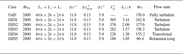
 Rem=2800
 λzf
 Reτ
 ν
 uτ

 τw
 E=∫0Lx∫−hh∫0Lz0.5ui′ui′dxdydz/(2hLxLz)
 τw
 ρUm2
 E
 uτ2
 t=t0
 Lz+=188

 u′
 v′
 kzE−u′v′(λz+,y+)
 σ−u′v′(λz+)
 λz+=188

 ⟨u⟩+
 −⟨u′v′⟩+
 λzf+
 Rem=2800
 λzf+
 Lz+=188
 uτ

 λzf+
 Rem=2800
 ⟨u′u′⟩+
 ⟨v′v′⟩+
 ⟨w′w′⟩+
 λzf+
 Lz+=188
 uτ

 kxEu′u′+(λx+,y+)
 kzEu′u′+(λz+,y+)
 ⋅
 ⋅
 …..
 ⋅⋅
 ⋅⋅
 +
 uτ

 kxEv′v′+(λx+,y+)
 kxEw′w′+(λx+,y+)
 kxE−u′v′+(λx+,y+)
 ⋅
 ⋅
 …..
 ⋅⋅
 ⋅⋅
 +
 uτ

 ⟨uiLujL⟩+
 ⟨uiSujS⟩+
 λzf+
 uτ

 Q=2
 u′
 y+=15
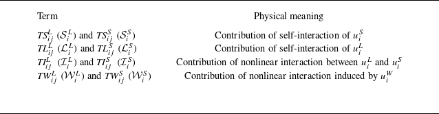

 ⟨uiLujL⟩
 uτ4/ν

 ⟨uiSujS⟩
 uτ4/ν

 ⟨uiSujS⟩
 ⟨uiLujL⟩
 TIijS
 TSijL
 TW33L

 ⟨uiSujS⟩¯xz+
 ⟨uiLujL⟩¯xz+
 0⩽y+⩽70
 ⟨⟩xz
 t=t0

 ⟨uiSujS⟩
 λzf+
 ⋅
 ⋅
 …..
 ⋅⋅
 ⋅⋅
 TW11S+
 TW22S+

 ⟨uiLujL⟩
 λzf+
 ⋅
 ⋅
 …..
 ⋅⋅
 ⋅⋅
 TW33L+

 τw
 Rem=11000
 t=t0

 ⟨uiLujL⟩+
 ⟨uiSujS⟩+
 λzf+
 Rem=11000
 uτ

 kxkzEu′u′¯+(λx+,λz+)
 kxkzEv′v′¯+(λx+,λz+)
 kxkzEw′w′¯+(λx+,λz+)
 0⩽y+⩽70
 ⋅
 ⋅
 …..
 λx≈10λz

 ⟨uiLujL⟩

 ⟨uiSujS⟩

 Rem=11000
 Rem=2800
 kzEu′u′+(λz+,y+)
 kzEv′v′+(λz+,y+)
 kzEw′w′+(λz+,y+)
 kzE−u′v′+(λz+,y+)
 kzEu′u′+
 kzEv′v′+
 y≈0.1λz
 y≈0.5λz
 λz+=200

 ⟨u⟩+
 ⟨u′u′⟩+
 ⟨v′v′⟩+
 ⟨w′w′⟩+

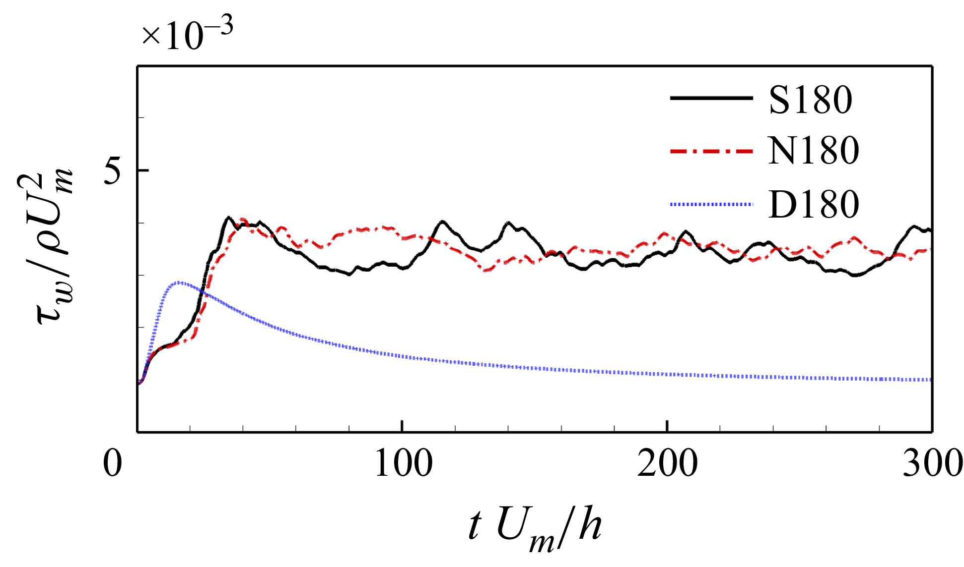
 τw

 Reτ=590
 λxf+
 t=t0

 ⟨uiLujL⟩lc+
 ⟨uiSujS⟩lc+
 λzf+
 uτ

 ⟨uiLujL⟩
 ⟨uiSujS⟩
 λx+⩾1000
 λz+⩽120
 λx+<1000
 λz+⩽120

 TW33L
 TW133L
 TW233L
 TW333L
 λx+⩾1000
 λz+⩽200
 λx+⩾1000
 λz+⩽120

 Open access

