1. INTRODUCTION
Automatic Identification System (AIS) base stations and coastal radar stations have been established in many coastal regions, generating a large amount of ship information every day. This includes not only static information such as ship type, tonnage, country, etc., but also dynamic information, such as time, location, direction, speed, and so on. Under normal circumstances, the real-time status of maritime vessels can be identified easily based on the above information, but marine traffic and ship behaviour patterns can also be deduced from historical data, so as to facilitate maritime supervision, abnormal behaviour detection and port infrastructure construction. However, some vessels with AIS cheat detection by turning off transponders, falsifying position data, or deliberately transmit improper identification data to evade detection for illegal operations or even illegal exploration (McCauley et al., Reference McCauley, Woods, Sullivan, Bergman, Jablonicky, Roan, Hirshfield, Boerder and Worm2016). In addition, there are still such problems as data quality and radar target recognition. For these reasons, it is often very difficult to find out the true type or identity of some ships in the historical database, which not only poses a challenge in marine surveillance and maritime security defence, but also interferes with further data mining. Therefore, it has become an important task to classify and identify these unknown vessels correctly.
In recent years, the study of the classification and prediction of moving objects by using data mining technology and massive trajectory data (Zheng, Reference Zheng2015; Feng and Zhu, Reference Feng and Zhu2016) has become common. For instance, with regard to the classification of ground moving objects, such as pedestrians, bicycles and cars, Dodge et al. (Reference Dodge, Weibel and Forootan2009) extracted global and local movement features from trajectories and took the Support Vector Machine (SVM) approach to train the classification model, which was used to predict the object type of unknown trajectories. Considering the classification and prediction of hurricane trajectories, Patel et al. (Reference Patel, Sheng, Hsu and Lee2012) and Patel (Reference Patel2013) proposed not only to take the spatial distributions and shapes of trajectories as features, but also to extract the duration-aware features from trajectories for building a classifier, achieving higher accuracy of classification than before.
Other researchers classified and predicted the activity patterns of moving objects by combining trajectory features with geographic and semantic information. For example, Zhu et al. (Reference Zhu, Zheng, Zhang, Santani, Xie and Yang2011) aimed to infer the status of a taxi, consisting of Occupied, Non-occupied, and Parked, according to its trajectories, so they partitioned trajectories using a stay-point detection method, and then extracted from each segment a set of features based on historical trajectories, road networks and Points Of Interest (POI). After that, they used the identified features to train a local probabilistic classifier and then globally considered travel patterns via a hidden semi-Markov model. Boukhechba et al. (Reference Boukhechba, Bouzouane, Bouchard, Gouinvallerand and Giroux2015) presented an approach capable of incrementally extracting semantic locations from the trajectories of pedestrians, and achieved real-time classification and prediction of users' activity types based on an online K-means algorithm.
Currently, most research on ship trajectory data focuses on marine traffic pattern mining, ship collision risk assessment, and maritime anomaly detection (Aarsæther and Moan, Reference Aarsæther and Moan2009; Silveira et al., Reference Silveira, Teixeira and Guedes Soares2013; Zhen et al., Reference Zhen, Jin, Hu, Shao and Nikitakos2017), but few researchers pay attention to ship classification. Lee et al. (Reference Lee, Han, Li and Gonzalez2008) proposed a trajectory classification method using hierarchical region-based and trajectory-based clustering after trajectory partitioning. Regardless of the movement patterns, they first utilised region-based clustering to discover regions in which trajectories mostly belong to one class. Subsequently, trajectory-based clustering (Lee et al., Reference Lee, Han and Whang2007) was employed to discover sub-trajectories indicating common movement patterns of each class. By using the collaboration between two types of clustering, they could discover two types of discriminative features for identifying the type of the moving objects. Nevertheless, this method did not consider the essential differences between different types of moving objects. During the classification of ship types, this method worked efficiently only in regions where types of ships clearly differed, such as the vicinity of harbours or in fisheries. De Vries and Van Someren (Reference De Vries and Van Someren2012; Reference De Vries and Van Someren2014) first compressed trajectories through two-stage piecewise linear segmentation to retain stop and move information. Then, they defined trajectory similarities based on compressed trajectories as kernels, and used them in a kernel method (such as SVM) for ship classification. If a ship arrives in a new area or where such types of ships have rarely appeared before, it is much more likely to be wrongly classified. However, this classification method is not suitable for ships sailing on a wide ranged sea area with a high degree of freedom. Elwakdy et al. (Reference Elwakdy, El-Bendary and Eltokhy2015) extracted the polynomial coefficients of sub-trajectories as trajectory features after trajectory segmentation and polynomial fitting, and built a ship classifier based on an Adaptive Neuropathy-Fuzzy Inference System (ANFIS). The advantage of this method is to utilise the innate shape characteristics of trajectories to avoid the influence of the geographical spaces of the ships. However, the temporal dimension is discarded, and it is required that segments of the same amount are divided from different types and lengths of ship trajectories. It is therefore difficult to ensure all trajectories can be partitioned properly when the data set is large or the duration is long. Failure to do so may lead to a poor fitting result with complex trajectories and loss of many effective features for classification.
To identify the types of ships more accurately in a broader sea area, this paper utilises the Logistic Regression (LR) model, one of the most popular classification techniques in the machine learning domain, to classify the ships. The overall process of building the classification model is shown in Figure 1. First, the raw trajectory is split into anchored-off, straight-sailing, and turning sub-trajectories based on the proposed three basic movement patterns and the related sub-trajectory partitioning algorithms. Second, three categories of trajectory features are extracted from the sub-trajectories on the basis of the presented feature extraction methods. Third, the trajectory feature dataset is generated by analysing and selecting the extracted features. Last, the ship classifier is constructed by using the LR model. In this paper, a case study is shown on the building of a classification model for identifying fishing boats and cargo ships from real AIS data. Experimental results indicate that the proposed methods can well meet the needs of recognising unclear types of targets from historical trajectory data.
Overall process of building a ship classification model.

The rest of this paper is organised as follows. Section 2 briefly introduces the logistic regression classification algorithm. Section 3 proposes ship movement patterns with the related trajectory partitioning algorithm, and the trajectory feature extraction method. Section 4 presents an experiment on the classification of fishing boats and cargo ships based on real AIS data. Section 5 concludes the paper, and outlines potential future research.
2. LOGISTIC REGRESSION ALGORITHM
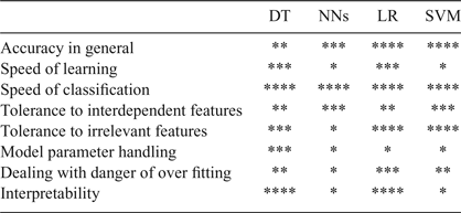
The problem of ship type recognition based on trajectory features can be attributed to the classification problem in the machine learning domain. There are many classification algorithms, such as the Decision Trees (DT), Artificial Neutral Networks (ANNs), Logistic Regression (LR) and Support Vector Machines (SVMs). As shown in Table 1, each algorithm has its own advantages and disadvantages and suitable scope of application (Kotsiantis, Reference Kotsiantis2007; Hastie et al., Reference Hastie, Tibshirani and Friedman2009; Harrington, Reference Harrington2012). Thanks to its advantages including high accuracy, simple mathematical model, easy programming and good interpretability, the logistic regression algorithm is chosen for our classification model. This section briefly introduces the logistic regression algorithm (Schein and Ungar, Reference Schein and Ungar2007; Zhou, Reference Zhou2016).
Comprehensive comparison of common classification algorithms.

(**** represents the best performance and * represents the worst)
2.1. Logistic regression classifier and sigmoid function
Logistic regression is a generalised linear model and is mainly used in two classification problems. We assume that the training dataset
 $\lcub \lpar x_{i1}\comma \; x_{i2}\comma \; x_{i3}\comma \; ...\comma \; x_{iN}\comma \; y_{i}\rpar \rcub _{i=1}^{M}$
is given,
 $X=\lpar x_{1} \comma \; x_{2} \comma \; x_{3} \comma \; ...\comma \; x_{n}\rpar \in R^{N}$
describes the N-dimensional feature vector and y is the classification label, whose value range is {0, 1}. We expect to build a linear regression model z = w
T
X + b for the classification boundary of the training set, and then map the predicted value z from
R
to a range between 0 and 1. Therefore, the sigmoid function is introduced:
 $$\sigma (z) = \displaystyle{{1}\over{1+e^{-z}}}$$
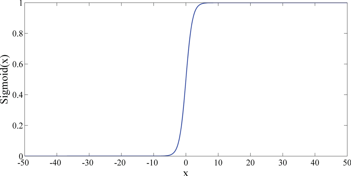
The sigmoid function curve is shown in Figure 2. When x = 0, the function value equals 0·5; with the increase of x, the function value will rapidly approach 1; and with the decrease of x, the value of σ(z) will rapidly approach 0. If the x-axis scale is large enough, the sigmoid function will be very similar to a step function, but the sigmoid function is easy to deal with in mathematics since it is continuously differentiable. To use this function as a classifier, we need to substitute the predicted value of the linear regression into it (see Equation 2) to obtain a result between 0 and 1, then any result bigger than 0·5 is put into the 1-class, otherwise it is put into the 0-class.
 $$y = \displaystyle{{1}\over{1+e^{-(w^TX+b)}}}$$
Sigmoid function curve.

2.2. Estimates of regression coefficients
If we see y in Equation (2) as the posterior probability of a result in the 1-class occurring, then we get:
 $$P(y=1\vert X)=\pi (X)=\displaystyle{{1}\over{1+e^{-(w^TX+b)}}}$$
 $$P(y=0\vert X)=1-\pi (X)=\displaystyle{{1}\over{1+e^{(w^TX+b)}}}$$
Here we can use the maximum likelihood method to estimate w and b. For the given training dataset
 $\lcub \lpar x_{i1} \comma \; x_{i2} \comma \; x_{i3} \comma \; ...\comma \; x_{iN}\comma \; y_{i} \rpar \rcub _{i=1}^{M}$
, the likelihood function of the logistic regression model is:
 $$L(w,b)=\prod\limits_{i=1}^M {[\pi (X_i )]^{y_i} [1-\pi (X_i )]^{1-y_i}}$$
Then the log likelihood function is:
 $$l(w,b)=\ln L(w,b)=\sum\limits_{i=1}^M {(y_i \ln [\pi (X_i )]} +(1-y_i )\ln [1-\pi (X_i )])$$
Thus, the logistic regression model can be described as an optimisation problem as follows:
 $$(w,b)^\ast =\hbox{max} _{(w,b)} l(w,b)$$
If there are too many features, over-fitting may occur and the model will lose its generalisation ability. To prevent this phenomenon, a regular item is commonly added to the optimisation target to punish excessive parameters, e.g., the L1-norm (sum of absolute value of coefficients) and the L2-norm (sum of squares of coefficients). If we add the regular item L2-norm, the optimisation target becomes:
 $$(w,b)^{\ast} = \hbox{max}_{(w,b)} \{l(w,b)-\lambda \left \vert {(w,b)} \right \vert_2 \}$$
In Equation (8), the parameter λ is the regularisation coefficient. Let
 $\theta =\lpar w\comma \; b\rpar $
,
 $J\lpar \theta \rpar =l\lpar \theta \rpar -\lambda \Vert \theta \Vert _{2}$
; the gradient ascent method (or other methods) can be employed to find the maximum value of J(θ). Then, the optimal estimates of θ will be obtained. The iterative equation of the gradient ascent method is shown in Equation (9). The parameter α is the step length, and
 $\nabla_{\theta} J\lpar \theta\rpar $
is the functional derivative. This equation will be executed until a certain termination condition is reached.
 $$\theta: = \theta + \alpha \cdot \nabla_{\theta} J (\theta)$$
3. TRAJECTORY PARTITIONING ALGORITHM AND FEATURE EXTRACTION
Trajectory feature extraction provides a foundation for training the ship type classification model for ship types. In this section, the basic movement patterns of ships are presented first, and then the trajectory partitioning algorithms are designed. Finally, the trajectory feature extraction method is proposed.
3.1. Definition of basic movement patterns of ships
In the existing studies on trajectory data mining, most researchers only partition the trajectory into stop and move patterns (Li et al., Reference Li, Zheng, Xie, Chen, Liu and Ma2008; Yuan et al., Reference Yuan, Zheng, Zhang and Xie2013; Wang et al, Reference Wang, Zheng and Xue2014). However, unlike pedestrians, cars or other ground moving objects whose trajectories are restricted by the road network, ships sail on the sea almost unlimitedly, and almost every steering operation has a clear purpose. That is to say, turning is also an important pattern of movement in ship trajectories. On this basis, ship trajectories are divided into three basic patterns in this paper, that is, anchored-off, straight-sailing and turning.
Usually, a vessel anchored at sea has random displacement within a certain range, and there is always error in ship positioning. Hence, the trajectory speed is not necessarily zero when the ship is at rest. The anchored-off pattern of the ship trajectory is defined as follows:
-
• Definition 1: Anchored-off pattern. Assume that a ship trajectory is
 $T = \lcub p_{1}\comma \; p_{2}\comma \; p_{3}\comma \; ...\comma \; p_{n} \rcub $
, and p
i
is the trajectory point. If there is a sub-trajectory T′ ⊆ T, the speed of T′ is less than δ
v
, the duration is greater than δ
t
, and the distance between each pair of trajectory points in T′ is shorter than δ
d
, then the movement pattern of T′ is called the anchored-off pattern.

For the remaining parts of the trajectory T, their movement pattern is called the sailing pattern, but this can be further divided into the straight-sailing pattern and the turning pattern. In contrast to moving objects on land, the degree of freedom of the ship steering operation is higher, the steering direction may be adjusted back and forth, and the time cost is relatively higher. Thus, the trajectory corresponding to a steering operation is a complex curve. At the same time, the direction may be changed slightly when a ship is sailing on the sea, but this is not discussed in this paper. For this reason, some thresholds are required for filtering. The turning pattern is therefore defined as follows:
-
• Definition 2: Turning pattern. Set the turning threshold as
$\Delta_{\theta}$
. If the total value of the direction changes before or after a trajectory point p
i
within a certain time range Δ
t1 is greater than
$\Delta_{\theta}$
, p
i
is called the possible turning point. If there are several continuous possible turning points and the duration is larger than the threshold Δ
t2, the movement pattern of the sub-trajectory consisting of those possible turning points is called the turning pattern. -
• Definition 3: Straight-sailing pattern. The movement pattern of the remaining parts excluding anchored-off and turning pattern trajectories is the so-called straight-sailing pattern. The three defined basic movement patterns of ship trajectory are shown in Figure 3.


Basic movement patterns of ship trajectory.

3.2. Trajectory partitioning algorithm
According to the basic movement patterns defined in Section 3.1, this section studies how to split a trajectory into anchored-off, turning, and straight-sailing sub-trajectories. First, the SplitTrajs algorithm is designed to split a complete ship trajectory into anchored-off and sailing sub-trajectories. After that, the SplitSailingTrajs algorithm is designed to split the sailing sub-trajectory into turning and straight-sailing segments.
3.2.1. SplitTrajs algorithm
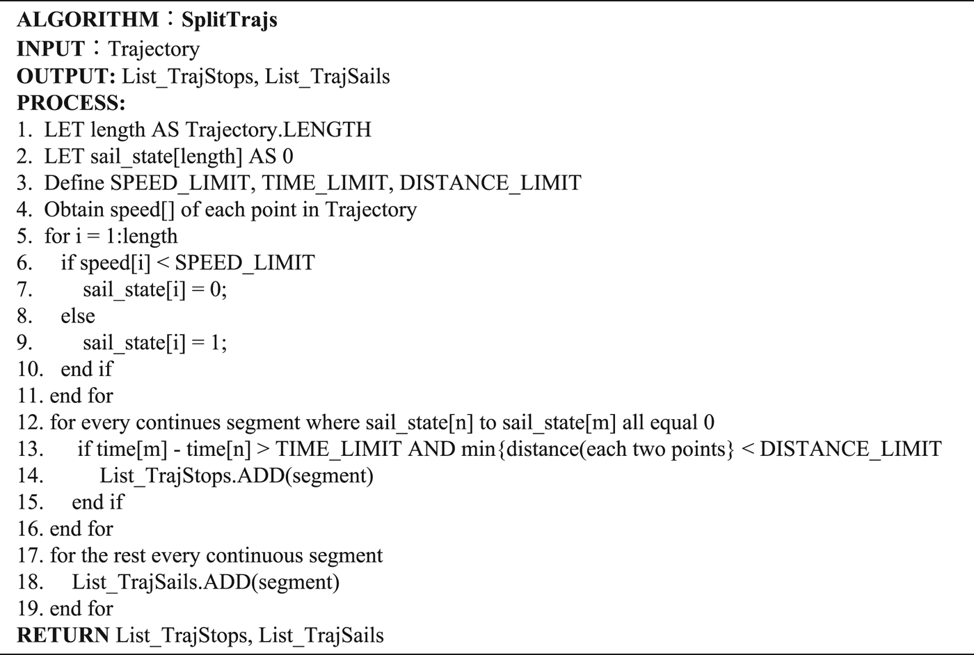
The SplitTrajs algorithm detects the trajectory points in anchored-off patterns from the given trajectory based on the velocity threshold δ v , the duration threshold δ t and the distance threshold δ d , which are mentioned in Definition 1. Then the trajectory is partitioned into anchored-off and sailing sub-trajectories. The pseudo-code of this algorithm is shown in Figure 4.
SplitTrajs pseudo-code

The input parameter of SplitTrajs is a ship trajectory, and the outputs are a list of anchored-off segments, named List_TrajStops, and a list of sailing segments, named List_TraSails. In the handling process, the total number of the trajectory points is defined as length and the array sail_state is initialised to represent the sailing state of each trajectory point. Based on Definition 1, the thresholds δ v (SPEED_LIMIT), δ t (TIME_LIMIT) and δ d (DISTANCE_LIMIT) are set and initialised (lines 1 ~ 3). Next, the velocity of each trajectory point is calculated and recorded in the array speed. Then each value in speed is compared with SPEED_LIMIT. If the ith value in this array is less than SPEED_LIMIT, then the ith value of array sail_state is set to 0; otherwise it is set to 1 (lines 4 ~ 10). Third, the segments whose corresponding array sail_state continuously has values of 1 are removed. If the interval of one segment is greater than TIME_LIMIT and the distance between each pair of points is shorter than DISTANCE_LIMIT, this segment is then in an anchored-off pattern and it will be added to the List_TrajStops (lines 11 ~ 16). Finally, the remaining segments are added in List_TraSails (lines 17 ~ 19).
3.2.2. SplitSailingTrajs algorithm
According to Definition 2, the SplitSailingTrajs algorithm detects all possible turning points first based on the turning threshold
 $\Delta_{\theta}$
and interval threshold Δ
t1, and then compares the segment consisting of continuously possible turning points to the duration threshold Δ
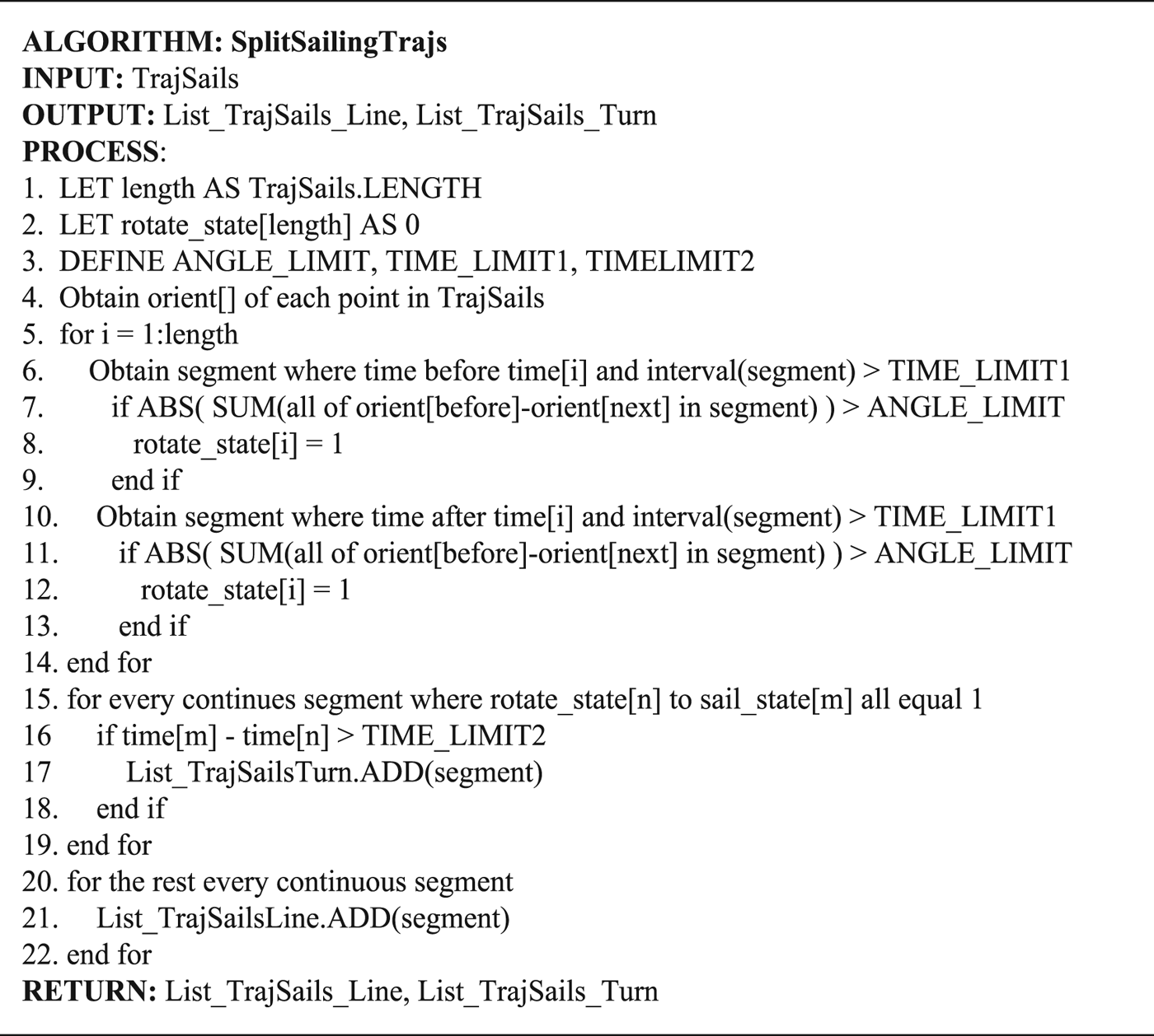
t2 to judge whether it is in a turning pattern. The pseudo-code of this algorithm is shown in Figure 5.
SplitSailingTrajs pseudo-code.

The input parameter of SplitSailingTrajs is the sailing sub-trajectory, and the outputs are a list of turning segments, named List_TrajSails_Turn, and a list of straight-sailing segments, named List_TrajSails_Line. First, the total number of the points in the input segment is set as length; array rotate_state is initialised to represent the turning state of each trajectory point, and the thresholds
 $\Delta_{\theta}$
(ANGLE_LIMIT), Δ
t1 (TIME_LIMIT1) and Δ
t2 (TIME_LIMIT2) are set (lines 1 ~ 3). Second, the orientation of each trajectory point is calculated (line 4). Third, the total orientation changes in interval Δ
t1 before and after each point is computed. If any result of p
i
is greater than
 $\Delta_{\theta}$
, then it is marked as the possible turning point and the ith value of rotate_state is set to 1(lines 5 ~ 14). Subsequently, the parts where the corresponding value of rotate_state continuously has values of 1 are extracted. If the duration of any part is longer than TIME_LIMIT2, then it is in a turning pattern and it will be added to List_TrajSails_Turn (lines 16 ~ 19). Finally, the remaining trajectories are added to List_TrajSails_Line (lines 20 ~ 22).
The threshold parameters in the above algorithms can be determined based on expert experience or experimental results.
3.3. Trajectory feature extraction
To study ship classification based on massive trajectory datasets, as many features that can be used to distinguish the ship types are selected as possible. In this section, 17 types of trajectory features are extracted based on the basic movement patterns and the sub-trajectory segments proposed in Sections 3.1 and 3.2. These features can be divided into three categories, that is, global features, straight-sailing features and turning features.
3.3.1. Global features
Global features are extracted from all the anchored-off and sailing sub-trajectories, such as the stop times, average duration of stops, average speed of sailing, total sailing distance and the effective distance ratio. These features can reflect the overall characteristics of ship movement. The effective distance ratio is the ratio between the straight-line distance from the start to the end of the ship trajectory and the total sailing distance.
3.3.2. Straight-sailing features
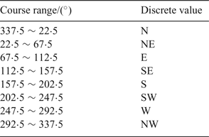
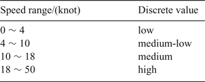
The straight-sailing features are extracted from the straight-sailing sub-trajectories, including the main course, main course sailing ratio, low speed sailing ratio, medium-low speed sailing ratio, medium speed sailing ratio and high-speed sailing ratio. To facilitate statistical analysis, it is necessary to discretise the course and speed values (Zhu et al., Reference Zhu, Zhang and Gao2012). Considering how ships actually navigate, the ship course is transformed into eight discrete values, and each of them is separated by 45° (see Table 2). Meanwhile, the ship sailing speed is also discretised into four catagories, which are low, medium-low, medium and high (Table 3).
Standard ship course discretisation.

Standard ship speed discretisation.

According to the discretisation, the features are defined as follows: the main course is the discrete value of ship course corresponding to the average direction of the longest straight-sailing segment. The main course sailing ratio is the ratio between the total distance of which directions are the same as main course among all the straight-sailing segments and the total sailing distance. The low speed sailing ratio is the ratio between the total time of sailing at low speed among all the straight-sailing segments and the total sailing time. The computation method for medium-low speed sailing ratio, medium speed sailing ratio and high speed sailing ratio is similar to the low speed sailing ratio.
3.3.3. Turning features
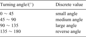
The turning features are extracted from the turning sub-trajectories, including the maximum turning speed, the maximum turning rate, small angle turn count, medium angle turn count, large angle turn count and reverse turn count. For convenience of statistical analysis, the turning angle is transformed into four discrete values as shown in Table 4.
The standard turning angle discretisation.

The calculation of turning features are as follows: Turning speed is the ratio between the turning distance and the turning time. Turning rate is the ratio between the total turning angle and the time of each turning segment. The small angle turn count means the total number of turns whose absolute value of direction changed is within the small angle range among all the turning sub-trajectories. The calculations of the medium angle turn count, large angle turn count and reverse turn count are similar to small angle turn count.
4. CASE STUDY
4.1. Data preparation
4.1.1. Raw data selection
In this paper, we select real AIS data from the sea area near Shantou, China (Longitude:
 $116^{\circ}\, \hbox{E} \sim 119^{\circ}\, \hbox{E}$
, Latitude:
 $21{\cdot}5^{\circ}\, \hbox{N} \sim 24{\cdot}5^{\circ}\, \hbox{N}$
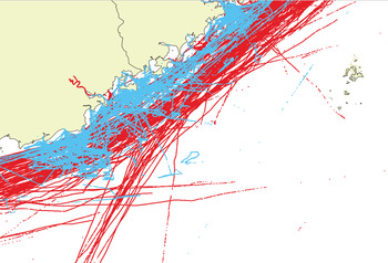
) from 1 to 7 October 2015. After data cleaning, data filtering and data transformation, AIS raw data is reconstructed into trajectory data and stored in the database. From the database, 1308 trajectories of fishing boats and cargo ships (654 each) are selected for training and testing the classification model as shown in Figure 6.
Fishing (blue) and cargo (red) trajectories near Shantou, China.

4.1.2. Ship sub-trajectory partitioning
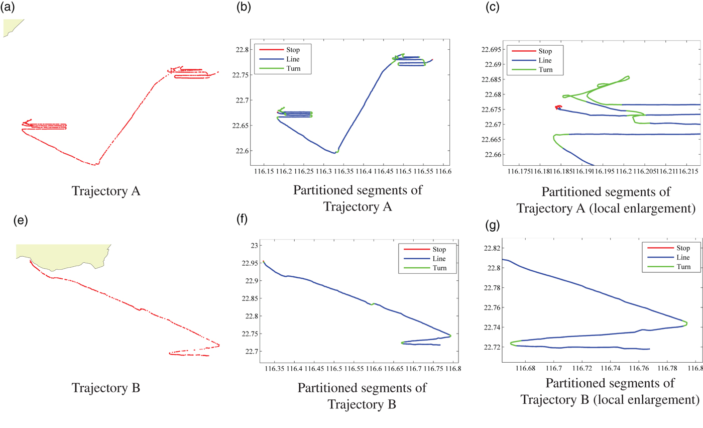
This paper realises the trajectory partitioning algorithm proposed in Section 3.2 by using the Java programming language. By adjusting the threshold parameters, the trajectories can be partitioned into anchored-off, turning and straight-sailing patterns with great accuracy. Some examples are given in Figure 7. On this basis, 10,571 fishing sub-trajectories and 3539 cargo sub-trajectories in total are obtained from the selected trajectories. The results are shown in Table 5.
Examples of trajectory partitioning based on real AIS data.

The standard turning angle discretisation.

4.1.3. Trajectory feature extraction and analysis
This paper extracts the trajectory features of fishing boats and cargo ships based on the feature extraction methods proposed in Section 3.3 and then builds the feature dataset. The results of trajectory feature analysis are shown in Figure 8.
Trajectory feature analysis and comparison of fishing boats (blue) and cargo ships (red).

As shown in Figure 8, the blue line represents the statistical characteristics of fishing boats, and the red line indicates cargo ships. The upper-left sub-graph shows the distribution of the global features by using a box-plot. In this figure, it is clear that cargo ships have Stop Times (ST), Average Duration of Stops (ADS), Average Speed of Sailing (ASS), total Sailing Distance (SD) and Effective Distance Ratio (EDR) longer or higher than fishing boats. The upper-right sub-graph compares the turning features between the trajectories of fishing boats and cargo ships. There is little difference in the Maximum Turning Speed (MTS) and Maximum Turning Rate (MTR) between such two types of ships in Figure 8, but the total turn count, including Small Angle Turn count (SAT), Medium Angle Turn count (MAT), Large Angle Turn count (LAT) and Reverse Angle Turn count (RAT) in fishing trajectories is significantly higher than for the cargo trajectories. In particular, the LAT and the RAT are more common in fishing boat trajectories, but rarely occur in cargo ship trajectories. The lower-left sub-graph shows the distribution of the main course of the fishing boats and cargo ships in our data. It is found that the main course of the cargo ships in this sea area is predominantly in the NE and SW directions, while that of the fishing boats is relatively uniform. Finally, in the lower-right sub-graph we include Main Course sailing Ratio (MCR), Low Speed sailing Ratio (LSR), Medium-Low Speed sailing Ratio (MLSR), Medium Speed sailing Ratio (MSR) and High Speed sailing Ratio (HSR). It is obvious that the cargo ships have a very high value of MCR, while the sailing speeds are very different between these two types of ships. Cargo ships are more likely to be sailing at the MLSR and MSR.
4.2. Ship classifier training based on logistic regression
Since this case is a binary classification problem, the logistic regression algorithm is chosen to train the ship trajectory classifier, with the aim of obtaining better predictions and explaining the obtained model. Today, the logistic regression algorithm has matured and has been integrated into a large number of data analysis and mining software packages. In this paper, the classification model is realised by using the Python 2.7 programming language in the Jupyter Notebook working environment, and the scientific computing environment is Anaconda (Pedregosa et al., Reference Pedregosa, Varoquaux, Gramfort, Michel and Thirion2012). The steps are as follows:
4.2.1. Feature selection and data conversion
Based on the feature extraction and analysis methods mentioned above, the two types of ships are not much different from each other in light of such features as maximum turning speed and maximum turning ratio, so the two features are removed to avoid interference. Additionally, features do not have consistent units, so the value of all the features are required to be normalised to 0 ~ 1 before use. Meanwhile, the classification targets need to be converted into two discrete values, so the class of fishing boat is set to 0 and that of cargo ship to 1.
4.2.2. Division into training and test data set
This paper utilises the hand-out method to divide the feature data set into two mutually exclusive sets, 75% to the training set and 25% to the test set. To improve the credibility of the model, this paper repeats the experiment 100 times to obtain 100 training sets and their correlated test sets.
4.2.3. Training and validation of classification model
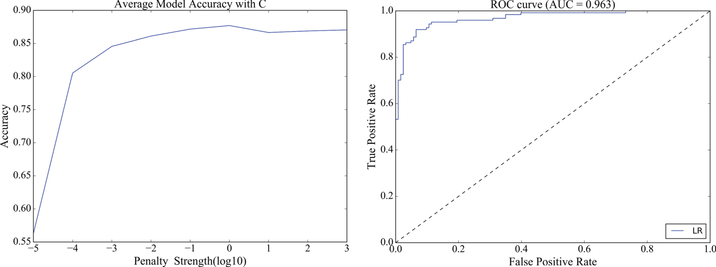
In the machine learning integration package scikit-learn in the Python environment, the logistic regression model usually requires three parameters, namely, loss function optimisation algorithm solver (the method for solving the optimisation target in Equation (8) such as the gradient ascent algorithm in Equation (9)), the penalty function penalty (the regular item in Equation (8) such as L1-norm and L2-norm) and the penalty strength C (the inverse of regularisation coefficient λ in Equation (8), with smaller values specifying greater penalties). Due to the small number of data set features, the coordinate descent algorithm (solver = ‘liblinear’) and L2 penalisation (penalty = ‘l2’) are chosen as the loss function optimisation method and the penalty function in this paper, so as to more accurately reflect the contribution of each feature to the final model (Scikit-learn User Guide, 2017). The penalty strength as a parameter needs to be determined experimentally. After a number of experiments (the average model accuracy with the change of C, shown in the left graph in Figure 9), the penalty strength is set to
 $1{\cdot}0\ \lpar C = 1{\cdot}0\rpar $
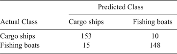
. Under this condition, the classification models are trained 100 times by using the training sets and validated by the corresponding test sets. The average correct rate of all the models is 0·877, the minimum is 0·834 and the maximum is 0·923. The model with the highest test accuracy is selected as the final classification model. The confusion matrix of the classification results of the final model is shown in Table 6.
Average model accuracy with the change of C (left) and the ROC curve of the optimal classifier (right).

Confusion matrix of the classification results.

In the binary classification problem, the Receiver Operation Characteristic (ROC) curve and the Area Under ROC Curve (AUC) are used to evaluate the performance of a classifier. The y-axis of the ROC curve is the True Positive Rate (TPR), which represents the proportion of the positive instances identified by the classifier to all positive instances. The x-axis is the False Positive Rate (FPR), which represents the proportion of negative instances that are divided into the positive class compared to all the negative instances. The ROC curve of a random classifier is the 45° diagonal line, and a perfect classifier has a ROC curve that through the upper left corner (0, 1). In general, the better the classifier, the closer its ROC curve is to the upper left corner. Figure 9 (right) shows the ROC curve of the ship classification model built in this paper. The curve of the classifier is very close to the upper left corner. AUC represents the classifier performance numerically. The AUC of a random classifier is 0·5 and a perfect one is equal to 1·0. By calculation, The AUC value of the final model is 0·963. Therefore, the ship classifier trained by using the presented method has high accuracy and reliability of prediction.
However, some ships are still misclassified. Through analysing raw trajectory data, most misclassified fishing boats sail at a relatively higher speed and the number of large or reverse angle turn count is relatively less. This may be due to fishing boats are not fishing, or they may be just transiting through the selected area for ocean fishing. Comparatively, most misclassified cargo ships are in the berthing state, or the actual sailing distance is very short, since the cargo ships are loading and unloading goods at the port. If the space-time trajectory of the ship is combined with the geographical knowledge and the semantic information is extracted as the classification features, it will be possible to further improve the accuracy of the classification results.
4.3. Result analysis
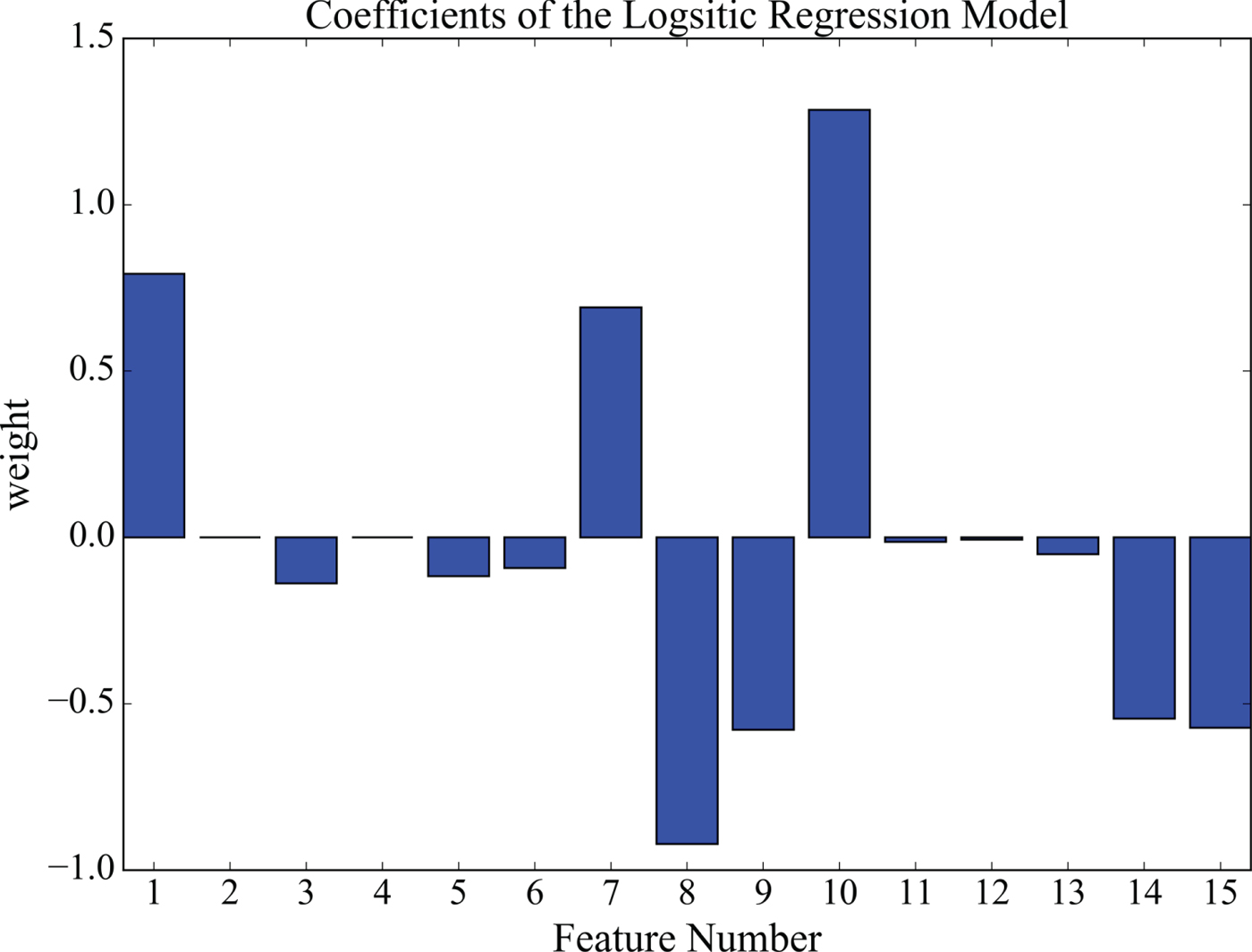
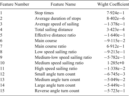
From the bar graph of the weight coefficient of the logistic regression model shown in Figure 10, the contribution of each feature to the ship classifier can be obtained. The positive weight value means this feature affects the cargo class more, while the negative value means the opposite. On the whole, seven out of 15 selected trajectory features are more important, that is, (in the descending order by the absolute value of the weight) medium speed sailing ratio, low speed sailing ratio, stop times, main course ratio, medium-low speed sailing ratio, reverse angle turn count, and the large angle turn count. The specific weight values of all the trajectory features are shown in Table 7.
The weight coefficients of logistic regression model (see Table 7 for Feature decode).

Weight coefficient of each feature in logistic regression model.

5. CONCLUSION
It is of great significance to identify the type of an unknown ship by its trajectory. This information can be used in many fields, such as camouflage identification, behaviour pattern mining and ship anomaly detection. To solve this problem, this paper makes three main contributions. Firstly, according to the characteristics of ship movement, three kinds of basic ship movement patterns are presented, and the partitioning algorithms for correlated sub-trajectories are designed. Secondly, three categories of ship trajectory features are put forward with their extraction methods. Finally, a ship classification model is built by using a logistic regression algorithm based on ship trajectory features.
Through the verification by use of real AIS data, the classification method proposed in this paper can satisfactorily address the classification problem of fishing boats and cargo ships based on their trajectories. However, there is still some work for the future. First of all, more features can be extracted from ship trajectories, such as acceleration and acceleration duration. Generally speaking, the more features, the more accurate the classifier is. Second, the semantic trajectory features can be extracted by combining with the geographic background and ship behaviour patterns and used in the training of future classification models. Third, this paper focuses only on the binary classification problem of ships, but it can be extended to solve the multi-classification problem, so that the research achievement can be better applied in practice. Moreover, the proposed method in this paper only considers off-line applications, but it may be extended for real-time ship classification in two possible ways. One is to dynamically extract the trajectory features of the unknown ships within a defined time window, and then classify and predict the ship type on the basis of the existing ship classification model. The other is to use the incremental learning techniques to modify the ship classifier constantly based on the online data to further improve its timeliness and reliability.